Good Subnetworks Provably Exist: Pruning via Greedy Forward Selection

The last few years have witnessed the remarkable success of large-scale deep neural networks (DNNs) in achieving human-level accuracy on complex cognitive tasks, including image classification (He et al. 2016, e.g.,), speech recognition (Amodei et al. 2016, e.g.,) and machine translation (Wu et al. 2016, e.g.,). However, modern large-scale DNNs tend to suffer from slow inference speed and high energy cost, which form critical bottlenecks on edge devices such as mobile phones and Internet of Things (IoT) (Cai et al. 2019). It is of increasing importance to obtain DNNs with small sizes and low energy costs.

Network pruning has been shown to be a successful approach for learning small and energy-efficient neural networks (Han et al. 2016b, e.g.,). These methods start with a pre-trained large neural network and remove the redundant units (neurons or filters/channels) to obtain a much smaller subnetwork without significant drop of accuracy. See e.g., Zhuang et al. 2018; Luo et al. 2017; Liu et al. 2017; Liu et al. 2019b; He et al. 2019; He et al. 2018b for examples of recent works.

However, despite the recent empirical successes, thorough theoretical understandings on why and how network pruning works are still largely missing. Our work is motivated by the following basic questions:

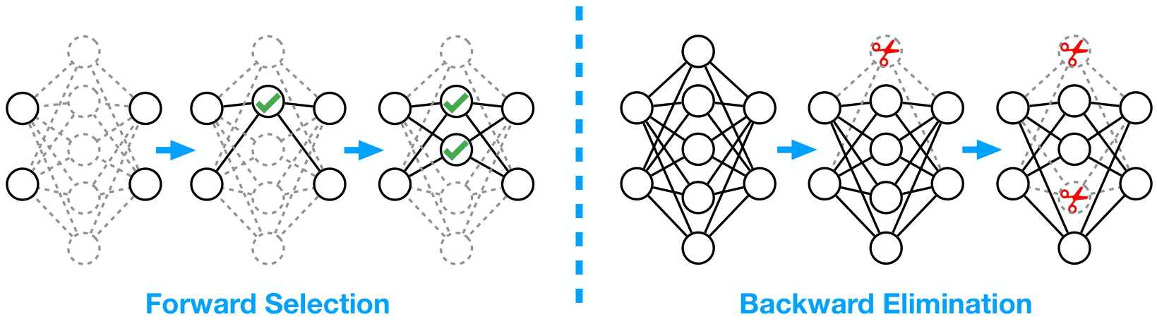We approach this problem by considering a simple greedy selection strategy, which starts from an empty network and constructs a good subnetwork by sequentially adding neurons from the pre-trained large network to yield the largest immediate decrease of the loss (see Figure 1(left)). This simple algorithm provides both strong theoretical guarantees and state-of-the-art empirical results, as summarized below.

We focus on two-layer networks for analysis. Assume we are given a pre-trained large neural network consisting of $N$ neurons,

where $\sigma(\bm{x};\textbf{$\bm{\theta}$}_{i})$ denotes the $i$-th neuron with parameter $\textbf{$\bm{\theta}$}_{i}\in\mathbb{R}^{d}$ and input $\bm{x}$. In this work, we consider

where $\textbf{$\bm{\theta}$}_{i}=[\bm{a}_{i},b_{i}]$ and $\sigma_{+}(\cdot)$ is an activation function such as Tanh and ReLU. But our algorithm works for general forms of $\sigma(\bm{x};\textbf{$\bm{\theta}$}_{i})$. Given an observed dataset $\mathcal{D}_{m}:=(\bm{x}^{(i)},y^{(i)})_{i=1}^{m}$ with $m$ data points, we consider the following regression loss of network $f$:

We are interested in finding a subset $S$ of $n$ neurons ($n<N$) from the large network, which minimizes the loss of the subnetwork $f_{S}(\bm{x})=\sum_{i\in S}\sigma(\bm{x};\textbf{$\bm{\theta}$}_{i})/|S|$, i.e.,

Here we allow the set $S$ to contain repeated elements. This is a challenging combinatorial optimization problem. We propose a greedy forward selection strategy, which starts from an empty network and gradually adds the neuron that yields the best immediate decrease on loss. Specifically, starting from $S_{0}=\emptyset$, we sequentially add neurons via

Notice that the constructed subnetwork inherits the weights of the large network and in practice we may further finetune the subnetwork with training data. More details of the practical algorithm and its extension to deep neural networks are in Section 4.

The simple greedy procedure yields strong theoretical guarantees, which, as a byproduct, also implies the existence of small and accurate subnetworks. Our results are two fold:

i) Under mild conditions, the selected subnetwork of size $n$ achieves $\mathcal{L}[f_{S_{n}}]=\mathcal{O}(1/n)+\mathcal{L}_{N}^{*}$, where $\mathcal{L}_{N}^{*}$ is the best possible loss achievable by convex combinations of all the $N$ neurons in $f_{[N]}$.

ii) We achieve a faster rate of $\mathcal{L}[f_{S_{n}}]=\mathcal{O}(1/n^{2})$ if the large network $f_{[N]}$ is sufficiently over-parameterized and can overfit the training data subject to small perturbation (see Assumption 2).

In comparison, the mean field analysis of Song et al. 2018; Mei et al. 2019 shows that:

iii) Training a network of size $n$ using (continuous time) gradient descent starting from random initialization gives an $\mathcal{O}(1/n+\varepsilon)$ loss, where $\varepsilon$ is a (typically small) term involving the loss of infinitely wide networks trained with gradient dynamics. See Song et al. 2018; Mei et al. 2019 for details.

Our fast $\mathcal{O}(1/n^{2})$ rate shows that subnetwork selection from large, over-parameterized models yields provably better results than training small networks of the same size starting from scratch using gradient descent. This provides the first theoretical justification of the empirical successes of the popular network pruning paradigm.

We now introduce the theory in depth. We start with the general $\mathcal{O}(1/n)$ rate in Section 3.1, and then establish and discuss the faster $\mathcal{O}(1/n^{2})$ rate in Section 3.2 and 3.3.

Structured Pruning A vast literature exists on structured pruning (Han et al. 2016a, e.g.,), which prunes neurons, channels or other units of neural networks. Compared with weight pruning (Han et al. 2016b, e.g.,), which specifies the connectivity of neural networks, structured pruning is more realistic as it can compress neural networks without dedicated hardware or libraries. Existing methods prune the redundant neurons based on different criterion, including the norm of the weights (Liu et al. 2017; Zhuang et al. 2018; Li et al. 2017, e.g.,), feature reconstruction error of the next or final layers (He et al. 2017; Yu et al. 2018; Luo et al. 2017, e.g.,), or gradient-based sensitivity measures (Baykal et al. 2019b; Zhuang et al. 2018, e.g.,). Our method is designed to directly minimize the final loss, and yields both better practical performance and theoretical guarantees.

Forward Selection vs. Backward Elimination Many of the popular conventional network pruning methods are based on backward elimination of redundant neurons (Liu et al. 2017; Li et al. 2017; Yu et al. 2018, e.g.), and fewer algorithms are based forward selection like our method (Zhuang et al. 2018, e.g.). Among the few exceptions, Zhuang et al. 2018 propose a greedy channel selection algorithm similar to ours, but their method is based on minimizing a gradient-norm based sensitivity measure (instead of the actual loss like us), and yield no theoretical guarantees. Appendix 11 discusses the theoretical and empirical advantages of forward selection over backward elimination.

Sampling-based Pruning Recently, a number of works (Baykal et al. 2019a; Liebenwein et al. 2019; Baykal et al. 2019b; Mussay et al. 2020) proposed to prune networks based on variants of (iterative) random sampling according to certain sensitivity score. These methods can provide concentration bounds on the difference of output between the pruned networks and the full networks, which may yield a bound of $\mathcal{O}(1/n+\mathcal{L}[f_{[N]}])$ with a simple derivation. Our method uses a simpler greedy deterministic selection strategy and achieves better rate than random sampling in the overparameterized cases In contrast, sampling-based pruning may not yield the fast $\mathcal{O}(1/n^{2})$ rate even with overparameterized models. Unlike our method, these works do not justify the advantage of pruning from large models over direct gradient training.

Lottery Ticket; Re-train After Pruning Frankle & Carbin 2019 proposed the Lottery Ticket Hypothesis, claiming the existence of winning subnetworks inside large models. Liu et al. 2019b regards pruning as a kind for neural architecture search. A key difference between our work and Frankle & Carbin 2019 and Liu et al. 2019b is how the parameters of the subnetwork are trained:

i) We finetune the parameters of the subnetworks starting from the weights of the pre-trained large model, hence inheriting the information the large model.

ii) Liu et al. 2019b proposes to re-train the parameters of the pruned subnetwork starting from new random initialization.

iii) Frankle & Carbin 2019 proposes to re-train the pruned subnetwork starting from the same initialization and random seed used to train the pre-trained model.

Obviously, the different parameter training of subnetworks should be combined with different network pruning strategies to achieve the best results. Our algorithmic and theoretical framework naturally justifies the finetuning approach. Different theoretical frameworks for justifying the proposals of Liu et al. 2019b and Frankle & Carbin 2019 (equipped with their corresponding subnetwork selection methods) are of great interest.

More recently, a concurrent work Malach et al. 2020 discussed a stronger form of lottery ticket hypothesis that shows the existence of winning subnetworks in large networks with random weights (without pre-training), which corroborates the empirical observations in (Wang et al. 2019; Ramanujan et al. 2019). However, the result of Malach et al. 2020 does not yield fast rate as our framework for justifying the advantage of network pruning over training from scratch, and does not motivate practical algorithms for finding good subnetworks in practice.

Frank-Wolfe Algorithm As suggested in Bach 2017, Frank-Wolfe (Frank & Wolfe 1956) can be applied to learn neural networks, which yields an algorithm that greedily adds neurons to progressively construct a network. However, each step of Frank-Wolfe leads to a challenging global optimization problem, which can not be solved in practice. Compared with Bach 2017, our subnetwork selection approach can be viewed as constraining the global optimization the discretized search space constructed using over-parameterized large networks pre-trained using gradient descent. Because gradient descent on over-parameterized networks is shown to be nearly optimal (Song et al. 2018; Mei et al. 2019; Du et al. 2019b; Du et al. 2019a; Jacot et al. 2018, e.g.,), selecting neurons inside the pre-trained models can provide a good approximation to the original non-convex problem.

Sub-modular Optimization An alternative general framework for analyzing greedy selection algorithms is based on sub-modular optimization (Nemhauser et al. 1978). However, our problem 1 is not sub-modular, and the (weak) sub-modular analysis (Das & Kempe 2011) can only bound the ratio between $\mathcal{L}[f_{S_{n}}]$ and the best loss of subnetworks of size $n$ achieved by (1), not the best loss $\mathcal{L}_{N}^{*}$ achieved by the best convex combination of all the $N$ neurons in the large model.

We propose a simple and efficient greedy selection algorithm for constructing subnetworks from pretrained large networks. Our theory provably justifies the advantage of pruning from large models over training small networks from scratch. The importance of using sufficiently large, over-parameterized models and finetuning (instead of re-training) the selected subnetworks are emphasized. Empirically, our experiments verify our theory and show that our method improves the prior arts on pruning various models such as ResNet-34 and MobileNetV2 on Imagenet.

Suppose we train the network with $n$ neurons for $T$ time using gradient descent with random initialization, i.e., the network we obtain is $f_{\rho_{T}^{n}}$ using the terminology in Section 3.3. As shown by Song et al. 2018; Mei et al. 2019, $\mathcal{L}[f_{\rho_{T}^{n}}]$ is actually $\mathcal{O}(1/n+\epsilon)$ with high probability, where $\epsilon=\mathcal{L}[f_{\rho_{T}^{\infty}}]$ is the loss of the mean field limit network at training time $T$. Song et al. 2018 shows that $\lim_{T\to\infty}\mathcal{L}[f_{\rho_{T}^{\infty}}]=0$ under some regularity conditions and this implies that if the training time $T$ is sufficient, $\mathcal{L}[f_{\rho_{T}^{\infty}}]$ is generally a smaller term compared with the $\mathcal{O}(1/n)$ term.

To generate the synthesis data, we first generate a neural network $f_{\text{gen}}(\bm{x})=\frac{1}{1000}\sum_{i=1}^{N}b_{i}\text{sigmoid}(\bm{a}_{i}^{\top}\bm{x})$, where $\bm{a}_{i}$ are i.i.d. sample from a 10 dimensional standard Gaussian distribution and $b_{i}$ are i.i.d. sample from a uniform distribution $\text{Unif}(-5,5)$. The training data $\bm{x}$ is also generated from a 10 dimensional standard Gaussian distribution. We choose $f_{\text{gen}}(\bm{x})=y$ as the label of data. Our training data consists of 100 data points. The network we use to fit the data is $f=\frac{1}{n}\sum_{i=1}^{n}b_{i}^{\prime}\text{tanh}(\bm{a}_{i}^{\prime\top}\bm{x})$. We use network with 1000 neurons for pruning and the pruned models will not be finetuned. All networks are trained for same and sufficiently large time to converge.

In this subsection, we display the results of applying our proposed algorithm to various model structures on CIFAR-10 and CIFAR-100. On CIFAR-10 and CIFAR-100, we apply our algorithm to the networks already pruned by network slimming (Liu et al. 2017) provided by Liu et al. 2019b and show that we can further compress models which have already pruned by the $L_{1}$ regularization. We apply our algorithm on the pretrained models, and finetune the model with the same experimental setting as ImageNet.

As demonstrated in Table 4, our proposed algorithm can further compress a model pruned by Liu et al. 2019b without or only with little drop on accuracy. For example, on the pretrained VGG19 on CIFAR-10, Liu et al. 2017 can prune 30% channels and get $93.81\%\pm 0.14\%$ accuracy. Our algorithm can prune 44% channels of the original VGG19 and get $93.78\%\pm 0.16\%$ accuracy, which is almost the same as the strong baseline number reported by Liu et al. 2019b.

Let $\phi_{j}(\textbf{$\bm{\theta}$})=\sigma(\bm{x}^{(j)},\textbf{$\bm{\theta}$})/\sqrt{m}$ and $\bm{\phi}(\textbf{$\bm{\theta}$})=\left[\phi_{1}(\textbf{$\bm{\theta}$}),...,\phi_{m}(\textbf{$\bm{\theta}$})\right]$ to be the vector of the outputs of the neuron $\sigma(\bm{x};\textbf{$\bm{\theta}$})$ scaled by $1/\sqrt{m}$, realized on a dataset $\mathcal{D}_{m}:=\{\bm{x}^{(j)}\}_{j=1}^{m}$. We call $\bm{\phi}(\textbf{$\bm{\theta}$})$ the feature map of $\bm{\theta}$. Given a large network $f_{[N]}(x)=\sum_{i=1}^{N}\sigma(\bm{x};\textbf{$\bm{\theta}$}_{i})/N$, define the marginal polytope of the feature map to be

where conv denotes the convex hull. Then it is easy to see that Assumption 2 is equivalent to saying that $\textbf{y}:=[y^{(1)},\ldots,y^{(m)}]/\sqrt{m}$ is in the interior of the marginal polytope $\mathcal{M}_{N}$, i.e., there exists $\gamma>0$ such that $\mathcal{B}\left(\textbf{y},\gamma\right)\subseteq\mathcal{M}_{N}$. Here we denote by $\mathcal{B}\left(\bm{\mu},r\right)$ the ball with radius $r$ centered at $\bm{\mu}$. Similar to Assumption 2, Assumption 5 is equivalent to require that $\mathcal{B}\left(\textbf{y},\gamma^{*}\right)\subseteq\mathcal{M}$, where

We may further relax the assumption to assuming y is in the relative interior (instead of interior) of $\mathcal{M}_{N}$ and $\mathcal{M}$. However, this requires some refined analysis and we leave this as future work.

It is worth mention that when $\mathcal{M}$ has dimension $m$ and $f_{\rho_{T}^{\infty}}$ gives zero training loss, then assumption 5 holds. Similarly, if $\mathcal{M}_{N}$ has dimension $m$ and $f_{\rho_{T}^{N}}$ gives zero training loss, then assumption 2 holds.

Our theoretical analysis is also applicable for pruning randomly weighted networks. Here we give the following corollary.

This corollary is a special case of Theorem 3 when taking the training time to be zero ($T=0$). And as the network is not trained, Assumption 4 are not needed for this corollary.

A greedy backward elimination can be developed analogous to our greedy forward selection, in which we start with the full network and greedily eliminate neurons that gives the smallest increase in loss. Specifically, starting from $S_{0}^{\text{B}}=[N]$, we sequentially delete neurons via

where $\setminus$ denotes set minus. In this section, we demonstrate that the forward selection has significant advantages over backward elimination, from both theoretical and empirical perspectives.

Our proofs use the definition of the convex hulls defined in Section 9 of Appendix.

References

- Amodei et al. (2016) Amodei, D., Ananthanarayanan, S., Anubhai, R., Bai, J., Battenberg, E., Case, C., Casper, J., Catanzaro, B., Cheng, Q., Chen, G., et al. Deep speech 2: End-to-end speech recognition in english and mandarin. In International conference on machine learning, pp. 173–182, 2016.
- Araújo et al. (2019) Araújo, D., Oliveira, R. I., and Yukimura, D. A mean-field limit for certain deep neural networks. arXiv preprint arXiv:1906.00193, 2019.
- Bach (2017) Bach, F. Breaking the curse of dimensionality with convex neural networks. The Journal of Machine Learning Research, 18(1):629–681, 2017.
- Bach et al. (2012) Bach, F., Lacoste-Julien, S., and Obozinski, G. On the equivalence between herding and conditional gradient algorithms. International Conference on Machine, 2012.
- Baykal et al. (2019a) Baykal, C., Liebenwein, L., Gilitschenski, I., Feldman, D., and Rus, D. Data-dependent coresets for compressing neural networks with applications to generalization bounds. The International Conference on Learning Representations, 2019a.
- Baykal et al. (2019b) Baykal, C., Liebenwein, L., Gilitschenski, I., Feldman, D., and Rus, D. Sipping neural networks: Sensitivity-informed provable pruning of neural networks. arXiv preprint arXiv:1910.05422, 2019b.
- Cai et al. (2019) Cai, H., Zhu, L., and Han, S. Proxylessnas: Direct neural architecture search on target task and hardware. The International Conference on Learning Representations, 2019.
- Chaudhuri & Dasgupta (2010) Chaudhuri, K. and Dasgupta, S. Rates of convergence for the cluster tree. In Advances in Neural Information Processing Systems, pp. 343–351, 2010.
- Chen et al. (2012) Chen, Y., Welling, M., and Smola, A. Super-samples from kernel herding. arXiv preprint arXiv:1203.3472, 2012.
- Chin et al. (2019) Chin, T.-W., Ding, R., Zhang, C., and Marculescu, D. Legr: Filter pruning via learned global ranking. arXiv preprint arXiv:1904.12368, 2019.
- Das & Kempe (2011) Das, A. and Kempe, D. Submodular meets spectral: greedy algorithms for subset selection, sparse approximation and dictionary selection. In Proceedings of the 28th International Conference on International Conference on Machine Learning, pp. 1057–1064, 2011.
- Deng et al. (2009) Deng, J., Dong, W., Socher, R., Li, L.-J., Li, K., and Fei-Fei, L. Imagenet: A large-scale hierarchical image database. In 2009 IEEE conference on computer vision and pattern recognition, pp. 248–255. IEEE, 2009.
- Dong et al. (2017) Dong, X., Huang, J., Yang, Y., and Yan, S. More is less: A more complicated network with less inference complexity. In Proceedings of the IEEE Conference on Computer Vision and Pattern Recognition, pp. 5840–5848, 2017.
- Du et al. (2019a) Du, S. S., Lee, J. D., Li, H., Wang, L., and Zhai, X. Gradient descent finds global minima of deep neural networks. International Conference on Machine, 2019a.
- Du et al. (2019b) Du, S. S., Zhai, X., Poczos, B., and Singh, A. Gradient descent provably optimizes over-parameterized neural networks. International Conference of Learning Representations, 2019b.
- Dudley (1979) Dudley, R. M. Balls in rk do not cut all subsets of k+ 2 points. Advances in Mathematics, 31(3):306–308, 1979.
- Frank & Wolfe (1956) Frank, M. and Wolfe, P. An algorithm for quadratic programming. Naval research logistics quarterly, 3(1-2):95–110, 1956.
- Frankle & Carbin (2019) Frankle, J. and Carbin, M. The lottery ticket hypothesis: Finding sparse, trainable neural networks. The International Conference on Learning Representations, 2019.
- Han et al. (2015) Han, S., Pool, J., Tran, J., and Dally, W. Learning both weights and connections for efficient neural network. In Advances in neural information processing systems, pp. 1135–1143, 2015.
- Han et al. (2016a) Han, S., Liu, X., Mao, H., Pu, J., Pedram, A., Horowitz, M. A., and Dally, W. J. Eie: efficient inference engine on compressed deep neural network. ACM SIGARCH Computer Architecture News, 44(3):243–254, 2016a.
- Han et al. (2016b) Han, S., Mao, H., and Dally, W. J. Deep compression: Compressing deep neural networks with pruning, trained quantization and huffman coding. The International Conference on Learning Representations, 2016b.
- He et al. (2016) He, K., Zhang, X., Ren, S., and Sun, J. Deep residual learning for image recognition. In Proceedings of the IEEE conference on computer vision and pattern recognition, pp. 770–778, 2016.
- He et al. (2017) He, Y., Zhang, X., and Sun, J. Channel pruning for accelerating very deep neural networks. In Proceedings of the IEEE International Conference on Computer Vision, pp. 1389–1397, 2017.
- He et al. (2018a) He, Y., Kang, G., Dong, X., Fu, Y., and Yang, Y. Soft filter pruning for accelerating deep convolutional neural networks. International Joint Conference on Artificial Intelligence, 2018a.
- He et al. (2018b) He, Y., Lin, J., Liu, Z., Wang, H., Li, L.-J., and Han, S. Amc: Automl for model compression and acceleration on mobile devices. In Proceedings of the European Conference on Computer Vision (ECCV), pp. 784–800, 2018b.
- He et al. (2019) He, Y., Liu, P., Wang, Z., Hu, Z., and Yang, Y. Filter pruning via geometric median for deep convolutional neural networks acceleration. In Proceedings of the IEEE Conference on Computer Vision and Pattern Recognition, pp. 4340–4349, 2019.
- Howard et al. (2019) Howard, A., Sandler, M., Chu, G., Chen, L.-C., Chen, B., Tan, M., Wang, W., Zhu, Y., Pang, R., Vasudevan, V., et al. Searching for mobilenetv3. In Proceedings of the IEEE International Conference on Computer Vision, pp. 1314–1324, 2019.
- Jacot et al. (2018) Jacot, A., Gabriel, F., and Hongler, C. Neural tangent kernel: Convergence and generalization in neural networks. In Advances in neural information processing systems, pp. 8571–8580, 2018.
- Lacoste-Julien (2016) Lacoste-Julien, S. Convergence rate of frank-wolfe for non-convex objectives. NIPS, 2016.
- Li et al. (2017) Li, H., Kadav, A., Durdanovic, I., Samet, H., and Graf, H. P. Pruning filters for efficient convnets. The International Conference on Learning Representations, 2017.
- Liebenwein et al. (2019) Liebenwein, L., Baykal, C., Lang, H., Feldman, D., and Rus, D. Provable filter pruning for efficient neural networks. arXiv preprint arXiv:1911.07412, 2019.
- Liu et al. (2017) Liu, Z., Li, J., Shen, Z., Huang, G., Yan, S., and Zhang, C. Learning efficient convolutional networks through network slimming. In Proceedings of the IEEE International Conference on Computer Vision, pp. 2736–2744, 2017.
- Liu et al. (2019a) Liu, Z., Mu, H., Zhang, X., Guo, Z., Yang, X., Cheng, K.-T., and Sun, J. Metapruning: Meta learning for automatic neural network channel pruning. In Proceedings of the IEEE International Conference on Computer Vision, pp. 3296–3305, 2019a.
- Liu et al. (2019b) Liu, Z., Sun, M., Zhou, T., Huang, G., and Darrell, T. Rethinking the value of network pruning. The International Conference on Learning Representations, 2019b.
- Loshchilov & Hutter (2017) Loshchilov, I. and Hutter, F. Sgdr: Stochastic gradient descent with warm restarts. The International Conference on Learning Representations, 2017.
- Luo et al. (2017) Luo, J.-H., Wu, J., and Lin, W. Thinet: A filter level pruning method for deep neural network compression. In Proceedings of the IEEE international conference on computer vision, pp. 5058–5066, 2017.
- Malach et al. (2020) Malach, E., Yehudai, G., Shalev-Shwartz, S., and Shamir, O. Proving the lottery ticket hypothesis: Pruning is all you need, 2020.
- Mei et al. (2019) Mei, S., Misiakiewicz, T., and Montanari, A. Mean-field theory of two-layers neural networks: dimension-free bounds and kernel limit. arXiv preprint arXiv:1902.06015, 2019.
- Mussay et al. (2020) Mussay, B., Osadchy, M., Braverman, V., Zhou, S., and Feldman, D. Data-independent neural pruning via coresets. In The International Conference on Learning Representations, 2020.
- Nemhauser et al. (1978) Nemhauser, G. L., Wolsey, L. A., and Fisher, M. L. An analysis of approximations for maximizing submodular set functions—i. Mathematical programming, 14(1):265–294, 1978.
- Nguyen & Pham (2020) Nguyen, P.-M. and Pham, H. T. A rigorous framework for the mean field limit of multilayer neural networks, 2020.
- Ramanujan et al. (2019) Ramanujan, V., Wortsman, M., Kembhavi, A., Farhadi, A., and Rastegari, M. What’s hidden in a randomly weighted neural network? arXiv preprint arXiv:1911.13299, 2019.
- Sandler et al. (2018) Sandler, M., Howard, A., Zhu, M., Zhmoginov, A., and Chen, L.-C. Mobilenetv2: Inverted residuals and linear bottlenecks. In Proceedings of the IEEE Conference on Computer Vision and Pattern Recognition, pp. 4510–4520, 2018.
- Song et al. (2018) Song, M., Montanari, A., and Nguyen, P. A mean field view of the landscape of two-layers neural networks. Proceedings of the National Academy of Sciences, 115:E7665–E7671, 2018.
- Wang et al. (2019) Wang, Y., Zhang, X., Xie, L., Zhou, J., Su, H., Zhang, B., and Hu, X. Pruning from scratch. arXiv preprint arXiv:1909.12579, 2019.
- Wu et al. (2016) Wu, Y., Schuster, M., Chen, Z., Le, Q. V., Norouzi, M., Macherey, W., Krikun, M., Cao, Y., Gao, Q., Macherey, K., et al. Google’s neural machine translation system: Bridging the gap between human and machine translation. arXiv preprint arXiv:1609.08144, 2016.
- Yu et al. (2018) Yu, R., Li, A., Chen, C.-F., Lai, J.-H., Morariu, V. I., Han, X., Gao, M., Lin, C.-Y., and Davis, L. S. Nisp: Pruning networks using neuron importance score propagation. In Proceedings of the IEEE Conference on Computer Vision and Pattern Recognition, pp. 9194–9203, 2018.
- Zhuang et al. (2018) Zhuang, Z., Tan, M., Zhuang, B., Liu, J., Guo, Y., Wu, Q., Huang, J., and Zhu, J. Discrimination-aware channel pruning for deep neural networks. In Advances in Neural Information Processing Systems, pp. 875–886, 2018.
7 Details for the Toy Example
Suppose we train the network with neurons for time using gradient descent with random initialization, i.e., the network we obtain is using the terminology in Section 3.3. As shown by Song et al. 2018; Mei et al. 2019, is actually with high probability, where is the loss of the mean field limit network at training time . Song et al. 2018 shows that under some regularity conditions and this implies that if the training time is sufficient, is generally a smaller term compared with the term.