Ly$\alpha$ Blobs from Cold Streams Undergoing Kelvin-Helmholtz InstabilitiesLy$\alpha$ Blobs from Cold Streams Undergoing Kelvin-Helmholtz Instabilities–References0000

The shearing motion between the stream and the background induces KHI, which leads to the formation of a turbulent mixing region surrounding the stream²² 2 On a fundamental level, the mixing seen in the numerical simulations referenced here is artificial, since the viscous scale is not resolved. The mixing between the two phases is likely driven by turbulence that, by construction, cascades down to the viscosity length which is the same as the diffusion length. The diffusion scale depends on the Coloumb interaction length of an electron (its mean free path before Thompson scattering). At $\rho\sim 10^{-26}{\rm gr~cm^{-3}}$ and $T\sim 10^{5}\,{\rm K}$, this is approximately $10^{-3}\,{\rm pc}$. The assumption is that in reality, the fluids will eventually mix at this scale, and that the dissipation rate (through cooling) is conserved throughout the inertial range, explaining why the simulations are converged in terms of the total dissipation rate (Gronke & Oh 2018; Gronke & Oh 2020; Fielding et al. 2020; M20).. The typical density and temperature in this region are³³ 3 In practice, the mixing region contains a broad distribution of densities and temperatures rather than a charecteristic value (e.g. M20, figure 10). However, studies have shown that the evolution of the mixing region can be well described by considering a fluid with $\rho_{\rm mix}$ and $T_{\rm mix}$ as defined above (Gronke & Oh 2018; Gronke & Oh 2020; Ji, Oh & Masterson 2019; M20), though other studies have explored different characteristic densities and temperatures (Li et al. 2020; Hobbs & Feldmann 2020). It has also been shown that when the mixing region is well resolved, it maintains pressure equilibrium with the unmixed phases even as it cools (Fielding et al. 2020), consistent with the definitions of $\rho_{\rm mix}$ and $T_{\rm mix}$. (Begelman & Fabian 1990; Gronke & Oh 2018)

The cooling time in the mixing region is thus

where $\gamma$ is the adiabatic index of the gas, $k_{\rm B}$ is Boltzmann’s constant, $n_{\rm mix}$ is the particle number density in the mixing region, and $\Lambda(T_{\rm mix})$ is the cooling function evaluated at $T_{\rm mix}$.

In the non-radiative case (Padnos et al. 2018; Mandelker et al. 2019), the turbulent mixing layer expands into both the stream and the background and its width is well approximated by

where the dimensionless growth rate, $\alpha$, is (Dimotakis 1991)

with $M_{\rm tot}=V_{\rm s}/(c_{\rm s}+c_{\rm b})$. This approximation is an excellent fit for 2d planar slabs and also for 3d cylinders so long as $h\lower 2.58333pt\hbox{$\;\mathrel{\mathop{\kern 0.0pt\sim}\limits^{<}}\;$}R_{\rm s}$. We thus obtain the timescale for the mixing layer to grow to the size of the stream, i.e. $h=R_{\rm s}$,

For $\delta\sim 100$ and $M_{\rm b}\sim 1$, we get $\alpha\sim 0.05$ and $V_{\rm s}\sim 10c_{\rm s}$. In this case, $t_{\rm shear}$ is comparable to the stream sound crossing time,

M20 found that a key parameter for determining stream evolution is the ratio $t_{\rm cool,\,mix}/t_{\rm shear}$⁴⁴ 4 There is some controversy in the literature over whether the relevant cooling time is $t_{\rm cool,\,mix}$ or $t_{\rm cool,\,hot}$, i.e. the cooling time in the hot phase (Li et al. 2020). We here adopt $t_{\rm cool,\,mix}$, following Gronke & Oh 2018; Gronke & Oh 2020, and M20.. If $t_{\rm shear}<t_{\rm cool,\,mix}$, the evolution proceeds similarly to the non-radiative case studied by Mandelker et al. 2019, and the stream is eventually disrupted by KHI. However, if $t_{\rm cool,\,mix}<t_{\rm shear}$, then background gas entrained in the mixing layer cools and condenses onto the stream before it is disrupted by KHI. The stream thus remains cold, dense and collimated, and is not disrupted by hydrodynamic instabilities. Rather, the stream mass actually increases with time, as it entrains more and more gas from its hotter surroundings. Similar conclusions were reached in recent studies of high-velocity clouds in a hot CGM environment (Gronke & Oh 2018; Gronke & Oh 2020). The condition $t_{\rm cool,\,mix}=t_{\rm shear}$ leads to a critical stream radius,

where $T_{\rm s,4}=T_{\rm s}/10^{4}\,{\rm K}$, $n_{\rm s,0.01}=n_{\rm H,s}/0.01\,{\rm cm}^{-3}$, $\Lambda_{\rm mix,-22.5}=\Lambda(T_{\rm mix})/10^{-22.5}{\rm erg~s^{-1}~cm^{3}}$, $\delta_{100}=\delta/100$, and $\alpha_{0.1}=\alpha/0.1$.

The ratio $t_{\rm cool,\,mix}/t_{\rm shear}=(R_{\rm s}/R_{\rm s,crit})^{-1}$, so streams with $R_{\rm s}>R_{\rm s,crit}$ grow in mass rather than dissolve. M20 derived an approximate expression for the entrainment rate of hot gas onto the stream. The cold mass-per-unit-length (hereafter line-mass) as a function of time is given by⁵⁵ 5 See Gronke & Oh 2020 for a similar expression for the case of spherical cold clouds.

where $m_{0}=\pi R_{\rm s}^{2}\rho_{\rm s}$ is the initial stream line-mass, and we have introduced the entrainment timescale,

where $t_{\rm cool,s}$ is the cooling time at the stream temperature and density. In practice, M20 assumed the stream to be in thermal equilibrium with a UV background, so the net cooling time at $T_{\rm s}$ is formally infinite. Therefore, $t_{\rm cool,s}$ is replaced by $t_{\rm cool,1.5T_{\rm s}}$, the cooling time at $T=1.5T_{\rm s}$, which is roughly the minimal cooling time. However, M20 note that any temperature in the range $\sim(1.2-2)T_{\rm s}$ works equally well. The density is given by assuming pressure equilibrium.

As more mass is entrained in the flow, conservation of momentum causes the stream to decelerate. The velocity of the stream as a function of time is well approximated by⁶⁶ 6 When $t_{\rm cool,\,mix}<t_{\rm shear}$, the entrained background material very rapidly mixes with the stream material (M20, figures 3 and 12). In this case, the whole stream moves at roughly $V_{\rm s}$, save for a very narrow region near the outer edge of the mixing region where the velocity quickly drops to 0 towards the background. When $t_{\rm cool,\,mix}\lower 2.15277pt\hbox{$\;\mathrel{\mathop{\kern 0.0pt\sim}\limits^{>}}\;$}t_{\rm shear}$, the velocity distribution is much wider, and there can be a strong velocity gradient between the stream axis and its interface.

This reduces the kinetic energy per-unit-length associated with bulk laminar flow, which is well fit by

In addition to the stream losing kinetic energy, the background gas entrained by the stream loses thermal energy, at a rate per-unit-length of

where $e_{\rm b}=P/[(\gamma-1)\rho_{\rm b}]$ is the thermal energy per unit mass of the background fluid which is larger than that in the cold component by a factor $\delta\gg 1$, $\gamma=5/3$ is the adiabatic index of the gas, and $c_{\rm b}^{2}=\gamma P/\rho_{\rm b}$ is the adiabatic sound speed in the background. In the final equation we have used eq. (9) to approximate ${\dot{m}}$.

M20 found that the cooling radiation emitted per-unit-length by the stream is very well approximated by

The factor $5/3$ accompanying $\dot{E}_{\rm th}$ accounts for the fact that the pressure of the background gas just outside the mixing layer remains roughly constant, and therefore the condensation of background gas onto the stream is well approximated as an isobaric cooling flow. In this case, the emitted radiation is given by the difference in enthalpy, rather than energy, between the initial and final states (Fabian 1994). In eq. (14) we have ignored any net heating of the stream, which is found to be very small (M20). For stream temperatures of order $T_{\rm s}\sim 10^{4}\,{\rm K}$ and background temperatures of order $T_{\rm b}\sim 10^{6}\,{\rm K}$, roughly half the luminosity is emitted at temperatures $T<5\times 10^{4}\,{\rm K}$, and is thus expected to contribute substantially to Ly$\alpha$ radiation (M20).

The stream velocity as it enters the halo is proportional to the virial velocity, $V_{0}=\eta V_{\rm v}$, with $0.5\lower 2.58333pt\hbox{$\;\mathrel{\mathop{\kern 0.0pt\sim}\limits^{<}}\;$}\eta\lower 2.58333pt\hbox{$\;\mathrel{\mathop{\kern 0.0pt\sim}\limits^{<}}\;$}1$ (Goerdt & Ceverino 2015). The maximal value $\eta$ is likely to obtain is $\sqrt{2}$ if the stream enters the halo at the escape velocity. The virial velocity and radius at $z\lower 2.58333pt\hbox{$\;\mathrel{\mathop{\kern 0.0pt\sim}\limits^{>}}\;$}1$ are given by (Dekel et al. 2013)

with $M_{12}=M_{\rm v}/10^{12}{\rm M}_{\odot}$ and $(1+z)_{3}=(1+z)/3$. The halo temperature at $R_{\rm v}$ is proportional to the virial temperature, $T_{\rm h}=\Theta_{h}T_{\rm v}$, with $\Theta_{\rm h}\lower 2.58333pt\hbox{$\;\mathrel{\mathop{\kern 0.0pt\sim}\limits^{>}}\;$}3/8$ given by the jump conditions at the virial shock (Dekel & Birnboim 2006), though it may be larger due to additional heating by feedback from the central or satellite galaxies, or when the virial shock propagates outwards. The virial temperature is given by

The sound speed in the halo is

where we have assumed that $\mu_{\rm h}\sim 0.6$, appropriate for fully ionized gas with roughly primordial composition. The stream Mach number upon entering the halo is thus

Taking uncertainties in $\eta$ and $\Theta_{\rm h}$ into account, we have that $0.75\lower 2.58333pt\hbox{$\;\mathrel{\mathop{\kern 0.0pt\sim}\limits^{<}}\;$}M_{\rm b}\lower 2.58333pt\hbox{$\;\mathrel{\mathop{\kern 0.0pt\sim}\limits^{<}}\;$}2.25$.

If the stream is in thermal equilibrium with the UV background at $z\sim 2$, its temperature is $T_{\rm s}\sim 1.5\times 10^{4}$ (M20), with a mild dependence on density and metallicity. In practice, the temperature can be lower if the stream is self-shielded, or higher if the stream is highly turbulent before entering the halo, with turbulent dissipation timescales comparable to the cooling time. We therefore assume $T_{\rm s}=\Theta_{\rm s}1.5\times 10^{4}\,{\rm K}$, with $\Theta_{\rm s}\sim 0.5-2$⁷⁷ 7 We note that much lower values of $\Theta_{\rm s}$ could be possible if the stream were dense enough and/or metal-rich enough to allow cooling to much lower temperatures in less than a halo crossing time. While this may be the case at $z>5$, it is unlikely to occur at redshifts $z<4$ unless the metallicity in the stream is $\sim 0.1Z_{\odot}$ (Mandelker et al. 2018). This is very high compared to values found in cosmological simulations and observed in both LABs and Lyman limit systems at these redshifts.. The sound speed in the stream is

with $\mu_{\rm s,0.6}=\mu_{\rm s}/0.6$. If the stream is strongly self-shielded and predominantly neutral, then $\mu_{\rm s,0.6}\sim 2$. Assuming the stream and the hot halo are in pressure equilibrium, the density contrast is given by

Taking into account uncertainties in $\Theta_{\rm h}$ and $\Theta_{\rm s}$, density contrasts of $\delta\sim(30-300)$ are reasonable for a $M_{\rm v}\sim 10^{12}{\rm M}_{\odot}$ halo at $z\sim 2$.

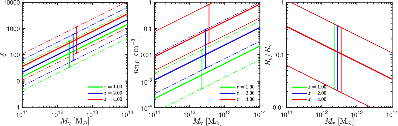
The stream density upon entering the halo virial radius, $\rho_{0}$, is given by the density contrast, $\delta$, and the density of the hot halo gas at $R_{\rm v}$. The latter is given by

where ${\overline{\rho}_{\rm h}}$ is the mean density of the hot component in the halo, ${\overline{\rho}_{\rm u}}(z)$ is the mean density of the universe at redshift $z$, $f_{\rm b}\simeq 0.17$ is the universal baryon fraction, and $f_{\rm h}$ denotes the fraction of the baryonic mass within the halo which is in the hot gas component. Simulations suggest this is $0.3\lower 2.58333pt\hbox{$\;\mathrel{\mathop{\kern 0.0pt\sim}\limits^{<}}\;$}f_{\rm h}\lower 2.58333pt\hbox{$\;\mathrel{\mathop{\kern 0.0pt\sim}\limits^{<}}\;$}0.4$ for halo masses $M_{12}\sim(0.5-2)$ at redshift $z\lower 2.58333pt\hbox{$\;\mathrel{\mathop{\kern 0.0pt\sim}\limits^{>}}\;$}2$ (Roca-Fàbrega et al. 2019), while observations of $M_{12}\sim(1-10)$ halos at $z\lower 2.58333pt\hbox{$\;\mathrel{\mathop{\kern 0.0pt\sim}\limits^{>}}\;$}0.1$ suggest $f_{\rm h}\sim 0.2-0.3$ (Singh et al. 2018). We define $f_{\rm h,0.3}=f_{\rm h}/0.3$. $\Delta(R_{\rm v})$ is the ratio of the density at $R_{\rm v}$ to the mean density in the halo, ${\overline{\rho}_{\rm v}}=3M_{\rm v}/(4\pi R_{\rm v}^{3})$. For a singular isothermal sphere $\Delta(R_{\rm v})=1/3$, while for an NFW halo with concentration $c=(5,10,20)$, $\Delta(R_{\rm v})\sim(0.24,0.19,0.14)$ respectively. We write $\Delta_{1/6}=\Delta(R_{\rm v})/(1/6)$. Assuming cosmological parameters $\Omega_{\rm m}=0.3$ and $H_{0}=70\,{\rm km/s/Mpc}$, we obtain for the stream density at $R_{\rm v}$

where $\delta_{100}=\delta/100$, and ${\widetilde{f}}_{\rm h}=\Delta_{1/6}f_{\rm h,0.3}\sim(1-3)$. For a Hydrogen mass fraction of $X=0.76$ this yields a Hydrogen number density in the stream at $R_{\rm v}$ of

We hereafter write $n_{\rm s,0.01}=n_{\rm H,0}/(0.01\,{\rm cm}^{-3})$.

The stream radius at $R_{\rm v}$ can be constrained using the mass flux through the stream,

where ${\dot{M}}_{\rm v}$ is the total mass accretion rate onto the halo virial radius, and $f_{\rm s}$ is the fraction of baryonic accretion along the gas stream. Cosmological simulations suggest $f_{\rm s}\sim(0.2-0.5)$ with a typical value of $f_{\rm s}=1/3$ (Danovich et al. 2012, i.e. three significant streams;). In the Einstein de Sitter (EdS) regime (valid at $z>1$), the accretion onto the virial radius is well approximated by Dekel et al. 2013

with halo-to-halo variance encapsulated by the normalization $s\sim(0.5-2)$. Combining eqs. (15), (23), (25), and (26), we obtain

with $\widetilde{s}=sf_{\rm s}/(1/3)\sim(0.3-3)$. Together with eq. (16) we have

Note that this is larger by a factor $\sim 2$ than the corresponding equation (68) in Padnos et al. 2018, which seems to be due to a typo as it is consistent with their equation (67). Using eq. (21) for $\delta$, we see that $R_{\rm s}/R_{\rm v}\propto M_{\rm v}^{-1/3}$ and is independent of redshift. More massive halos are thus fed by relatively narrower streams compared to their virial radii. We hereafter substitute ${\cal R}_{\rm sv}\equiv R_{\rm s}/R_{\rm v}$.

The Hydrogen column density perpendicular to the stream axis is $N_{\rm H,0}=n_{\rm H,0}R_{\rm s}$. Using eqs. (24) and (27) this yields

For $10^{12}{\rm M}_{\odot}$ halos at $z\sim 2$, this is large enough for the streams to be largely self-shielded against the UV background if the neutral fraction is $x_{\rm HI}\lower 2.58333pt\hbox{$\;\mathrel{\mathop{\kern 0.0pt\sim}\limits^{>}}\;$}10^{-3}$. In collisional ionization equilibrium (CIE), this is true for $T_{\rm s}\lower 2.58333pt\hbox{$\;\mathrel{\mathop{\kern 0.0pt\sim}\limits^{<}}\;$}3\times 10^{4}\,{\rm K}$ (Goerdt et al. 2010, e.g.), i.e. $\Theta_{\rm s}\lower 2.58333pt\hbox{$\;\mathrel{\mathop{\kern 0.0pt\sim}\limits^{<}}\;$}2$. Of course, streams may still be susceptible to local sources of UV radiation, such as star-formation in satellite galaxies located along the stream, or starbursts/AGN activity in the central galaxy.

References

- Arrigoni Battaia et al. (2019) Arrigoni Battaia F., Hennawi J. F., Prochaska J. X., Oñorbe J., Farina E. P., Cantalupo S., Lusso E., 2019, MNRAS, 482, 3162
- Arrigoni Battaia et al. (2018) Arrigoni Battaia F., Prochaska J. X., Hennawi J. F., Obreja A., Buck T., Cantalupo S., Dutton A. A., Macciò A. V., 2018, MNRAS, 473, 3907
- Aung et al. (2019) Aung H., Mandelker N., Nagai D., Dekel A., Birnboim Y., 2019, MNRAS, 490, 181
- Begelman & Fabian (1990) Begelman M. C., Fabian A. C., 1990, MNRAS, 244, 26P
- Berlok & Pfrommer (2019) Berlok T., Pfrommer C., 2019, arXiv e-prints, arXiv:1904.02167
- Birnboim & Dekel (2003) Birnboim Y., Dekel A., 2003, MNRAS, 345, 349
- Birnboim, Padnos & Zinger (2016) Birnboim Y., Padnos D., Zinger E., 2016, ApJ, 832, L4
- Borisova et al. (2016) Borisova E. et al., 2016, ApJ, 831, 39
- Bouché et al. (2016) Bouché N. et al., 2016, ApJ, 820, 121
- Bouché et al. (2013) Bouché N., Murphy M. T., Kacprzak G. G., Péroux C., Contini T., Martin C. L., Dessauges-Zavadsky M., 2013, Science, 341, 50
- Cantalupo et al. (2014) Cantalupo S., Arrigoni-Battaia F., Prochaska J. X., Hennawi J. F., Madau P., 2014, Nature, 506, 63
- Ceverino, Dekel & Bournaud (2010) Ceverino D., Dekel A., Bournaud F., 2010, MNRAS, 404, 2151
- Danovich et al. (2015) Danovich M., Dekel A., Hahn O., Ceverino D., Primack J., 2015, MNRAS, 449, 2087
- Danovich et al. (2012) Danovich M., Dekel A., Hahn O., Teyssier R., 2012, MNRAS, 422, 1732
- Dekel & Birnboim (2006) Dekel A., Birnboim Y., 2006, MNRAS, 368, 2
- Dekel et al. (2009) Dekel A. et al., 2009, Nature, 457, 451
- Dekel et al. (2013) Dekel A., Zolotov A., Tweed D., Cacciato M., Ceverino D., Primack J. R., 2013, MNRAS, 435, 999
- Dijkstra, Haiman & Spaans (2006) Dijkstra M., Haiman Z., Spaans M., 2006, ApJ, 649, 14
- Dijkstra & Loeb (2009) Dijkstra M., Loeb A., 2009, MNRAS, 400, 1109
- Dimotakis (1991) Dimotakis P. E., 1991, Turbulent free shear layer mixing and combustion. Tech. rep.
- Fabian (1994) Fabian A. C., 1994, ARA&A, 32, 277
- Fardal et al. (2001) Fardal M. A., Katz N., Gardner J. P., Hernquist L., Weinberg D. H., Davé R., 2001, ApJ, 562, 605
- Faucher-Giguère et al. (2010) Faucher-Giguère C.-A., Kereš D., Dijkstra M., Hernquist L., Zaldarriaga M., 2010, ApJ, 725, 633
- Faucher-Giguère, Kereš & Ma (2011) Faucher-Giguère C.-A., Kereš D., Ma C.-P., 2011, MNRAS, 417, 2982
- Fielding et al. (2017) Fielding D., Quataert E., McCourt M., Thompson T. A., 2017, MNRAS, 466, 3810
- Fielding et al. (2020) Fielding D. B., Ostriker E. C., Bryan G. L., Jermyn A. S., 2020, ApJ, 894, L24
- Fumagalli et al. (2017) Fumagalli M. et al., 2017, MNRAS, 471, 3686
- Fumagalli et al. (2011) Fumagalli M., Prochaska J. X., Kasen D., Dekel A., Ceverino D., Primack J. R., 2011, MNRAS, 418, 1796
- Furlanetto et al. (2005) Furlanetto S. R., Schaye J., Springel V., Hernquist L., 2005, ApJ, 622, 7
- Geach et al. (2009) Geach J. E. et al., 2009, ApJ, 700, 1
- Geach et al. (2007) Geach J. E., Smail I., Chapman S. C., Alexand er D. M., Blain A. W., Stott J. P., Ivison R. J., 2007, ApJ, 655, L9
- Goerdt & Ceverino (2015) Goerdt T., Ceverino D., 2015, MNRAS, 450, 3359
- Goerdt et al. (2010) Goerdt T., Dekel A., Sternberg A., Ceverino D., Teyssier R., Primack J. R., 2010, MNRAS, 407, 613
- Goerdt et al. (2012) Goerdt T., Dekel A., Sternberg A., Gnat O., Ceverino D., 2012, MNRAS, 424, 2292
- Gronke & Oh (2018) Gronke M., Oh S. P., 2018, MNRAS, 480, L111
- Gronke & Oh (2020) Gronke M., Oh S. P., 2020, MNRAS, 492, 1970
- Haardt & Madau (1996) Haardt F., Madau P., 1996, ApJ, 461, 20
- Haiman & Rees (2001) Haiman Z., Rees M. J., 2001, ApJ, 556, 87
- Hennawi et al. (2015) Hennawi J. F., Prochaska J. X., Cantalupo S., Arrigoni-Battaia F., 2015, Science, 348, 779
- Hobbs & Feldmann (2020) Hobbs A., Feldmann R., 2020, arXiv e-prints, arXiv:2001.06012
- Ji, Oh & Masterson (2019) Ji S., Oh S. P., Masterson P., 2019, MNRAS, 487, 737
- Katz, Weinberg & Hernquist (1996) Katz N., Weinberg D. H., Hernquist L., 1996, ApJS, 105, 19
- Kereš et al. (2005) Kereš D., Katz N., Weinberg D. H., Davé R., 2005, MNRAS, 363, 2
- Kereš & Hernquist (2009) Kereš D., Hernquist L., 2009, ApJ, 700, L1
- Komatsu & Seljak (2001) Komatsu E., Seljak U., 2001, MNRAS, 327, 1353
- Laursen & Sommer-Larsen (2007) Laursen P., Sommer-Larsen J., 2007, ApJ, 657, L69
- Leclercq et al. (2017) Leclercq F. et al., 2017, A&A, 608, A8
- Li et al. (2020) Li Z., Hopkins P. F., Squire J., Hummels C., 2020, MNRAS, 492, 1841
- Mandelker et al. (2020) Mandelker N., Nagai D., Aung H., Dekel A., Birnboim Y., van den Bosch F. C., 2020, MNRAS, 494, 2641
- Mandelker et al. (2019) Mandelker N., Nagai D., Aung H., Dekel A., Padnos D., Birnboim Y., 2019, MNRAS, 484, 1100
- Mandelker et al. (2016) Mandelker N., Padnos D., Dekel A., Birnboim Y., Burkert A., Krumholz M. R., Steinberg E., 2016, MNRAS, 463, 3921
- Mandelker et al. (2018) Mandelker N., van Dokkum P. G., Brodie J. P., van den Bosch F. C., Ceverino D., 2018, ApJ, 861, 148
- Martin et al. (2014a) Martin D. C., Chang D., Matuszewski M., Morrissey P., Rahman S., Moore A., Steidel C. C., 2014a, ApJ, 786, 106
- Martin et al. (2014b) Martin D. C., Chang D., Matuszewski M., Morrissey P., Rahman S., Moore A., Steidel C. C., Matsuda Y., 2014b, ApJ, 786, 107
- Martin et al. (2016) Martin D. C., Matuszewski M., Morrissey P., Neill J. D., Moore A., Steidel C. C., Trainor R., 2016, ApJ, 824, L5
- Martin et al. (2019) Martin D. C. et al., 2019, Nature Astronomy, 372
- Matsuda et al. (2007) Matsuda Y., Iono D., Ohta K., Yamada T., Kawabe R., Hayashino T., Peck A. B., Petitpas G. R., 2007, ApJ, 667, 667
- Matsuda et al. (2004) Matsuda Y. et al., 2004, AJ, 128, 569
- Matsuda et al. (2006) Matsuda Y., Yamada T., Hayashino T., Yamauchi R., Nakamura Y., 2006, ApJ, 640, L123
- Matsuda et al. (2011) Matsuda Y. et al., 2011, MNRAS, 410, L13
- Mori, Umemura & Ferrara (2004) Mori M., Umemura M., Ferrara A., 2004, ApJ, 613, L97
- Nelson et al. (2016) Nelson D., Genel S., Pillepich A., Vogelsberger M., Springel V., Hernquist L., 2016, MNRAS, 460, 2881
- Nelson et al. (2013) Nelson D., Vogelsberger M., Genel S., Sijacki D., Kereš D., Springel V., Hernquist L., 2013, MNRAS, 429, 3353
- Nilsson et al. (2006) Nilsson K. K., Fynbo J. P. U., Møller P., Sommer-Larsen J., Ledoux C., 2006, A&A, 452, L23
- Ocvirk, Pichon & Teyssier (2008) Ocvirk P., Pichon C., Teyssier R., 2008, MNRAS, 390, 1326
- Ohyama et al. (2003) Ohyama Y. et al., 2003, ApJ, 591, L9
- Padnos et al. (2018) Padnos D., Mandelker N., Birnboim Y., Dekel A., Krumholz M. R., Steinberg E., 2018, ArXiv e-prints
- Palunas et al. (2004) Palunas P., Teplitz H. I., Francis P. J., Williger G. M., Woodgate B. E., 2004, ApJ, 602, 545
- Pezzulli & Cantalupo (2019) Pezzulli G., Cantalupo S., 2019, MNRAS, 486, 1489
- Prescott et al. (2008) Prescott M. K. M., Kashikawa N., Dey A., Matsuda Y., 2008, ApJ, 678, L77
- Prochaska, Lau & Hennawi (2014) Prochaska J. X., Lau M. W., Hennawi J. F., 2014, ApJ, 796, 140
- Rauch et al. (2008) Rauch M. et al., 2008, ApJ, 681, 856
- Roca-Fàbrega et al. (2019) Roca-Fàbrega S. et al., 2019, MNRAS, 484, 3625
- Saito et al. (2006) Saito T., Shimasaku K., Okamura S., Ouchi M., Akiyama M., Yoshida M., 2006, ApJ, 648, 54
- Singh et al. (2018) Singh P., Majumdar S., Nath B. B., Silk J., 2018, MNRAS, 478, 2909
- Smith & Jarvis (2007) Smith D. J. B., Jarvis M. J., 2007, MNRAS, 378, L49
- Springel (2010) Springel V., 2010, MNRAS, 401, 791
- Steidel et al. (2000) Steidel C. C., Adelberger K. L., Shapley A. E., Pettini M., Dickinson M., Giavalisco M., 2000, ApJ, 532, 170
- Steidel et al. (2011) Steidel C. C., Bogosavljević M., Shapley A. E., Kollmeier J. A., Reddy N. A., Erb D. K., Pettini M., 2011, ApJ, 736, 160
- Trebitsch et al. (2016) Trebitsch M., Verhamme A., Blaizot J., Rosdahl J., 2016, A&A, 593, A122
- van de Voort & Schaye (2012) van de Voort F., Schaye J., 2012, MNRAS, 423, 2991
- van de Voort et al. (2012) van de Voort F., Schaye J., Altay G., Theuns T., 2012, MNRAS, 421, 2809
- van de Voort et al. (2011) van de Voort F., Schaye J., Booth C. M., Haas M. R., Dalla Vecchia C., 2011, MNRAS, 414, 2458
- Vogelsberger et al. (2012) Vogelsberger M., Sijacki D., Kereš D., Springel V., Hernquist L., 2012, MNRAS, 425, 3024
- Weidinger, Møller & Fynbo (2004) Weidinger M., Møller P., Fynbo J. P. U., 2004, Nature, 430, 999
- Weidinger et al. (2005) Weidinger M., Møller P., Fynbo J. P. U., Thomsen B., 2005, A&A, 436, 825
- Wilman et al. (2005) Wilman R. J., Gerssen J., Bower R. G., Morris S. L., Bacon R., de Zeeuw P. T., Davies R. L., 2005, Nature, 436, 227
- Yang et al. (2010) Yang Y., Zabludoff A., Eisenstein D., Davé R., 2010, ApJ, 719, 1654
- Yang et al. (2009) Yang Y., Zabludoff A., Tremonti C., Eisenstein D., Davé R., 2009, ApJ, 693, 1579