On the Expected Backreaction During Preheating

Let us expand the inflaton field $\phi$ around such a homogeneous but otherwise arbitrary background, $\phi=\bar{\phi}+\delta{\phi}$. Expressed in terms of the fluctuations, the matter action becomes

$$\begin{split}S_{\mathrm{m}}=\int d^{4}x\sqrt{-g}\Big[&\left(\Box\bar{\phi}-\bar{V}^{\prime}\right)\delta\phi-\frac{1}{2}\partial_{\mu}\delta\phi\partial^{\mu}\delta\phi-\frac{1}{2}\bar{V}^{\prime\prime}\delta\phi^{2}\\ &-\frac{1}{2}\partial_{\mu}\chi\partial^{\mu}\chi-\frac{M_{0}^{2}+\bar{\lambda}}{2}\chi^{2}-\frac{\bar{\lambda}^{\prime}}{2}\,\delta\phi\,\chi^{2}-\frac{\bar{\lambda}^{\prime\prime}}{4}\,\delta\phi^{2}\,\chi^{2}+\cdots\Big].\end{split}$$

(3.2)

Here and in the following, a prime denotes a derivative with respect to $\phi$, and a bar over a function indicates evaluation at $\bar{\phi}$. Note that the term linear in $\delta\phi$ does not vanish because we do not assume that $\bar{\phi}$ satisfies its classical equation of motion.

The presence of couplings between $\delta\phi$ and $\chi$ indicates that the inflaton influences the dynamics of the matter fields. This is obvious from the effective mass of $\chi$, which depends on the background value of the inflaton through the coupling function $\bar{\lambda}$. Diagrammatically, this influence is captured by the self-energy diagrams in figure 2. These corrections could be inserted into any of the matter propagators in figure 1 to determine how they affect the production of gravitational waves. We restrict our attention to one-loop diagrams for simplicity.

As the inflaton oscillates around the minimum of its potential after the end of inflation, the mode functions of the matter field $\chi$ experience parametric resonance, whereas those of the inflaton field do not. Hence, we would expect the dominant self-energy contributions to arise from the diagram with matter, rather than the inflaton, in the loop. Alternatively, we could consider a theory in which the inflaton couples to $\mathcal{N}$ identical matter fields and restrict our attention to the leading contribution in a large $\mathcal{N}$ expansion. In either case, the dominant matter self-energy correction stems from the tadpole diagram for the inflaton in figure 2. Such tadpoles are absent if we demand the condition

$$\braket{\delta\phi}=0,$$

(3.3)

that is, when the sum of all diagrams with a single external $\delta\phi$ vanishes. Both in the $in$-$in$ and $in$-$out$ formalisms, demanding (3.3) is actually equivalent to the perhaps more familiar condition on the quantum effective action $\delta\Gamma/\delta\bar{\phi}=0,$ from which one typically derives the quantum-corrected equations of motion for the inflaton. If the background is such that condition (3.3) is satisfied, the impact of the inflaton on the evolution of the matter fields is mainly determined by its background field value $\bar{\phi}$. The enforcement of equation (3.3) as an alternative for the evaluation of the effective potential is known as “Weinberg’s tadpole method” [22].

In order to determine which background $\bar{\phi}$ fulfills equation (3.3), we shall simply evaluate the left hand side of equation (3.3) using the action in equation (3.2). Because we are not assuming that $\bar{\phi}$ satisfies the classical field equation, there is a non-zero interaction vertex linear in $\delta\phi$ and proportional to $\Box\bar{\phi}-\bar{V}^{\prime}$. Cancelling the $\delta\phi$ propagator we can thus cast the quantum corrected equation of motion as

	$$-\Box\bar{\phi}+\Braket{\frac{\partial V}{\partial\phi}}=0,$$		(3.4a)
where in the one-loop approximation
	$$\Braket{\frac{\partial V}{\partial\phi}}=\bar{V}^{\prime}+\frac{\bar{\lambda}^{\prime}}{2}\braket{\chi^{2}}.$$		(3.4b)

In this formula $\braket{\chi^{2}}\equiv\braket{\mathrm{in}|\chi^{2}|\mathrm{in}}$ is the expectation value of $\chi^{2}$, where the $\chi$’s are free fields. Clearly, the interaction with $\chi$ effectively changes the inflaton potential, as one may have expected. Because they are subdominant during preheating, and in order to keep our presentation unencumbered, we are neglecting inflaton self-interactions. The latter could be easily included in our analysis nevertheless. At one loop they would give an extra contribution $(1/2)\bar{V}^{\prime\prime\prime}\braket{\delta\phi^{2}}$ to the right-hand side of equation (3.4b). Note that we can identify the $in$-$in$ expectation of the field $\phi$ with its background value, $\braket{\mathrm{in}|\phi|\mathrm{in}}=\bar{\phi}$, because of condition (3.3). We shall refer to $\braket{\partial V/\partial\phi}$ as the “driving term.”

To study the evolution of the inflaton we thus need to evaluate the expectation of $\chi^{2}$. We expand the free field $\chi$ in creation and annihilation operators as usual,

$$\chi=\frac{1}{\sqrt{\mathcal{V}}}\sum_{\vec{k}}(w_{k}e^{i\vec{k}\cdot\vec{x}}a_{\vec{k}}+w_{k}^{*}e^{-i\vec{k}\cdot\vec{x}}a^{\dagger}_{\vec{k}}),$$

(3.5)

where $\mathcal{V}$ is the (finite) spatial volume of the universe, which we shall take to infinity momentarily. In the spacetime (3.1) the mode functions $w_{k}$ satisfy the mode equation

$$\ddot{w}_{k}+2\mathcal{H}\dot{w}_{k}+(k^{2}+a^{2}\kappa_{0})w_{k}=0,$$

(3.6)

where $\kappa_{0}\equiv M_{0}^{2}+\bar{\lambda}$ is the effective (inflaton-dependent) squared mass of the matter field $\chi$, $\mathcal{H}\equiv\dot{a}/a$ is the comoving Hubble scale, and a dot denotes a derivative with respect to conformal time. Then, assuming that matter is in the $in$ vacuum, $a_{\vec{k}}\ket{\mathrm{in}}=0$, we find

$$\langle{\chi^{2}}\rangle=\frac{1}{(2\pi)^{3}}\int d^{3}k\,|w_{k}|^{2},$$

(3.7)

where we have replaced the discrete mode sum by an integral. Note that $\braket{\chi^{2}}$ is spatially constant, as a consequence of the homogeneity of the cosmological background.

We shall regulate the divergent mode integral (3.7) with exactly the same methods described in reference [13], to which we refer the reader for further details. Essentially, the regularization entails the introduction of a set of $n$ Pauli-Villars regulator fields $\chi_{r}$ of Grassmann parity $\sigma_{r}$, with the same couplings as $\chi$, but with different masses $M_{r}$, where $r=1,\ldots n$. Because they couple like the original matter field $\chi\equiv\chi_{0}$, their effective squared masses are

$$\kappa_{i}\equiv M_{i}^{2}+\bar{\lambda},$$

(3.8)

and the actual expectation that enters the effective potential in equation (3.4b) is ${\braket{\chi^{2}}\equiv\sum_{i=0}^{n}\braket{\chi^{2}_{i}}}.$ At the end of the calculation we shall decouple the regulator fields by sending their masses $M_{r}$ to infinity, leaving a finite, renormalized theory behind.

We can identify the potentially divergent contributions in equation (3.7) by first introducing a cutoff at comoving momenta $k=\Lambda$ and then expanding the mode integrals in the number of time derivatives acting on the background. The key ingredient here is an analogous “adiabatic” expansion of the mode functions in the number of time derivatives. The latter is only valid at large values of $k$ or large values of $M_{r}^{2}$. Hence, we shall only be able to analytically recover the ultraviolet behavior of the original mode integral (3.7), or the magnitude of $\braket{\chi_{r}^{2}}$ when the regulators become sufficiently heavy. Fortunately, these are the only regimes we shall need to renormalize the divergences we shall encounter.

At zeroth-order in time derivatives we find

	$$\langle{\chi^{2}}\rangle^{(0)}=\frac{1}{4(2\pi^{2})}\sum_{i}\sigma_{i}\left[\frac{\Lambda^{2}}{a^{2}}+\frac{\kappa_{i}}{2}\left(1-\log x_{i}\right)\right],$$		(3.9a)
and at two derivatives we obtain
	$$\langle{\chi^{2}}\rangle^{(2)}=\frac{1}{24(2\pi^{2})}\sum_{i}\sigma_{i}\left[\bar{R}\left(-\frac{5}{6}+\frac{1}{2}\log x_{i}\right)+\frac{\mathcal{H}}{a^{2}}\frac{\dot{\kappa}_{i}}{\kappa_{i}}-\frac{\dot{\kappa}_{i}^{2}}{4a^{2}\kappa_{i}^{2}}+\frac{\ddot{\kappa}_{i}}{2a^{2}\kappa_{i}}\right],$$		(3.9b)

where we have introduced the dimensionless ratio

$$x_{i}\equiv\frac{4\Lambda^{2}}{a^{2}\kappa_{i}}$$

(3.10)

and used that for the metric (3.1) the Ricci scalar is $\bar{R}=6\ddot{a}/a^{3}$. In both equations (3.9), the expectation depends on $\bar{\phi}$ through the squared effective masses $\kappa_{i}$. Note that the leading divergent terms with no derivatives are proportional to the square of the cutoff or the field masses, whereas those with two derivatives are at most logarithmically divergent. On dimensional grounds, terms with higher derivatives remain finite as the cutoff $\Lambda$ is removed or the regulators are decoupled. Say, all terms with four derivatives remain finite in the limit $\Lambda\to\infty$; their form ranges from $H^{4}/\kappa_{i}$ to $\ddot{\kappa}^{2}_{i}/(a^{4}\kappa_{i}^{3})$, where $H\equiv\mathcal{H}/a$ is the Hubble constant.

From equations (3.9), as we send $\Lambda$ to infinity the mode integral remains finite if the regulator masses and parities obey

$$\sum_{i}\sigma_{i}=0,\quad\sum_{i}\sigma_{i}M_{i}^{2}=0.$$

(3.11)

This is possible because fermionic fields ($\sigma_{i}=-1$) give loop contributions with the opposite sign as those of bosonic fields ($\sigma_{i}=1$). If conditions (3.11) are satisfied the theory is finite, but the expectation still depends on the otherwise arbitrary regulator masses. Although $\braket{\chi^{2}}$ still appears to depend on the physical cutoff $\Lambda/a$ through $x_{i}$, this dependence cancels again because of equations (3.11), so we might as well replace $\Lambda/a$ in $x_{i}$ by any other mass scale.

The dependence on the regulator fields disappears if we decouple them by sending their masses to infinity, $M_{r}\to\infty$. Then, their only traces left are the divergent contributions stemming from the logarithms in equations (3.9). The latter happen to contribute to the effective equation of motion just like the counterterms

$$S_{\mathrm{ct}}\supset\int d^{4}x\sqrt{-g}\left[-\delta d_{1}\,\lambda(\phi)-\delta d_{2}\,\lambda^{2}(\phi)-\delta\xi\,\lambda(\phi)\,R\right],$$

(3.12)

which introduce additional corrections to the effective equation of motion of the inflaton field,

	$$-\Box\bar{\phi}+\Braket{\frac{\partial V}{\partial\phi}}_{\mathrm{ren}}=0,$$		(3.13a)
where we have identified the renormalized driving term with
	$$\Braket{\frac{\partial V}{\partial\phi}}_{\mathrm{ren}}\equiv\bar{V}^{\prime}+\frac{\bar{\lambda}^{\prime}}{2}\sum_{i}\braket{\chi_{i}^{2}}+\delta d_{1}\,\bar{\lambda}^{\prime}+2\delta d_{2}\,\bar{\lambda}\bar{\lambda}^{\prime}+\delta\xi\,\bar{\lambda}^{\prime}\,\bar{R}.$$		(3.13b)

Clearly, the counterterms proportional to $\delta d_{1}$ and $\delta d_{2}$ can be also thought of as part of the inflaton potential. The coefficients in equations (3.9) that diverge logarithmically as $M_{r}\to\infty$ are canceled by the counterterms, provided that the latter diverge like

	$\displaystyle 2\pi^{2}\delta d_{1}$	$\displaystyle=\frac{1}{16}\sum_{r}\sigma_{r}M_{r}^{2}\log X_{r}+\delta d^{f}_{1},$		(3.14a)
	$\displaystyle 2\pi^{2}\delta d_{2}$	$\displaystyle=\frac{1}{32}\sum_{r}\sigma_{r}\log X_{r}+\delta d^{f}_{2},$		(3.14b)
	$\displaystyle 2\pi^{2}\delta\xi$	$\displaystyle=-\frac{1}{96}\sum_{r}\sigma_{r}\log X_{r}+\delta\xi^{f}\ .$		(3.14c)

The yet undetermined and finite pieces of the counterterms are denoted by the superscript “$f$.” The log-divergent pieces force us to usher in an arbitrary inflaton scale $\bar{\phi}=\mu$ and the corresponding effective mass of matter at that scale,

$$\kappa_{\mu}\equiv M_{0}^{2}+\lambda(\mu),\quad X_{r}\equiv\frac{\kappa_{\mu}}{M_{r}^{2}}.$$

(3.15)

The counterterms (3.12) share the structure of the original action (2.1) only for particular choices of the coupling function $\lambda$. Say, if $\lambda$ is a polynomial of degree $n$, the counterterms introduce corrections to the inflaton potential of degree $2n$. This implies that renormalizability (in our limited context) demands the bare scalar field potential also be a polynomial of degree $2n$. The finite pieces of each of the coefficients in such a polynomial are then determined by appropriate renormalization conditions, as we explore below, whereas the divergent components follow from equations (3.14). If we assume that the scalar field potential is renormalizable in the traditional sense, $V$ can only be a quartic polynomial, and this restricts the coupling function to ${\lambda=\lambda_{1}\phi+\lambda_{2}\phi^{2}}$. There is no wave function renormalization at one loop, hence the absence of a counterterm proportional to the squared gradient of the inflaton.

As far as the terms with zero derivatives are concerned, our discussion parallels that of field theory in Minkowski spacetime. In particular, we have basically obtained the derivative of the Coleman-Weinberg effective potential in the theory defined by (2.1). Indeed, terms without time derivatives are not sensitive to the expansion of the universe, and should thus reproduce the Minkowski spacetime results. With the unrenormalized but regularized effective potential given by the integral over Euclidean four-momenta [23]

$$U_{CW}=\bar{V}+\frac{1}{2}\sum_{i}\sigma_{i}\int\frac{d^{4}p_{E}}{(2\pi)^{4}}\,\log\left(1+\frac{\kappa_{i}}{p_{E}^{2}}\right),$$

(3.16)

it is then easy to see that $dU_{CW}/d\bar{\phi}$ equals $\bar{V}^{\prime}+\frac{\bar{\lambda}^{\prime}}{2}\braket{\chi^{2}}^{(0)}$, in agreement with our calculation. Plugging the counterterms (3.14) into equation (3.13b) and taking the limit ${M_{r}\to\infty}$ we arrive at

$$\Braket{\frac{\partial V}{\partial\phi}}^{(0)}_{\mathrm{ren}}=\bar{V}^{\prime}+\frac{1}{2\pi^{2}}\left[\frac{(M_{0}^{2}+\bar{\lambda})\bar{\lambda}^{\prime}}{16}\log\frac{M_{0}^{2}+\bar{\lambda}}{M_{0}^{2}+\lambda(\mu)}+\delta d^{f}_{1}\,\bar{\lambda}^{\prime}+\left(2\delta d^{f}_{2}-\frac{1}{16}\right)\bar{\lambda}\bar{\lambda}^{\prime}\right].$$

(3.17)

Because the minimum of the inflaton potential is located at $\phi=0$, it would be natural to choose $\mu=0$ as renormalization point, but we would encounter then a zero-mass singularity when $M^{2}_{0}\to 0$. It is hence convenient to choose a non-zero $\mu$. Note that the presence of two arbitrary finite counterterms indicates that two conditions are necessary to fix the actual form of the driving term at zero derivatives.

But there is yet another contribution to the driving term at two derivatives that is sensitive to the ultraviolet, and forces the inflaton to couple non-minimally to gravity. It can be read off equations (3.13b), (3.9b) and (3.14c), which lead to

$$\Braket{\frac{\partial V}{\partial\phi}}^{(2)}_{\mathrm{ren}}=\frac{\bar{R}\bar{\lambda}^{\prime}}{2\pi^{2}}\left[\delta\xi^{f}-\frac{1}{48}\log\frac{M_{0}^{2}+\bar{\lambda}}{M_{0}^{2}+\bar{\lambda}(\mu)}\right].$$

(3.18)

The logarithmic dependence can be thought of as due to the running of the coupling constant $\delta\xi$ with the inflaton field. Even if $\delta\xi$ vanishes at $\bar{\phi}=\mu$, the running reintroduces the non-minimal coupling away from that value.

Yet it is also important to note that the quantum corrections that we have explicitly computed so far are only the first few terms in an infinite series. The renormalization conditions only affect the first two terms in such an expansion, but there is an infinite number of additional terms with higher derivatives that remain. Therefore, it is not sufficient to solely rely on the effective potential to discuss the impact of quantum corrections on the evolution of the inflaton. On dimensional grounds, the relative size of a correction with $2n$ time derivatives is expected to be of order $(H^{2}/\kappa_{0})^{n}$, and is thus likely to be negligible when $H^{2}\ll\kappa_{0}$. In order to go beyond such limit, it suffices to combine equations (3.9), (3.13b) and (3.14), which yield the “exact” renormalized driving term at one loop, valid at all orders in the derivative expansion,

	$\displaystyle\Braket{\frac{\partial V}{\partial\phi}}_{\mathrm{ren}}\!\!\!$	$\displaystyle=$	$\displaystyle\bar{V}^{\prime}+\frac{1}{2\pi^{2}}\Bigg\{\delta d^{f}_{1}\,\bar{\lambda}^{\prime}+\left(2\delta d^{f}_{2}-\frac{1}{16}\right)\bar{\lambda}\bar{\lambda}^{\prime}+\delta\xi^{f}\bar{\lambda}^{\prime}\,\bar{R}$		(3.19)
		$\displaystyle+$	$\displaystyle\frac{\bar{\lambda}^{\prime}}{2}\Bigg[\lim_{\Lambda\to\infty}\int_{0}^{\Lambda}\!\!\!dk\,k^{2}|w_{k}|^{2}-\frac{1}{4}\frac{\Lambda^{2}}{a^{2}}-\frac{\kappa_{0}}{8}\left(1-\log x_{\mu}\right)-\frac{\bar{R}}{24}\left(-\frac{5}{6}+\frac{1}{2}\log x_{\mu}\right)\Bigg]\Bigg\},$

where we have introduced the dimensionless ratio

$$x_{\mu}\equiv\frac{4\Lambda^{2}}{a^{2}\kappa_{\mu}}.$$

(3.20)

One advantage of our approach is that we are able to carry out the renormalization program while preserving diffeomorphism invariance and keeping the resulting expressions in a form suitable for numerical integration. Though diffeomorphism invariance has not played much a role so far, it is crucial in the analysis of the backreaction on the metric.

We have implemented the renormalization of the driving term numerically, by essentially following the same approach of reference [13]. The complete set of equations solved by our code is presented in appendix C. In this context, it is convenient to work with dimensionless quantities in a specific model. For illustration we choose the arguably simplest potential and coupling functions (C.10), which in the original variables read

$$V=\frac{1}{2}m_{\phi}^{2}\phi^{2},\quad\lambda=\lambda_{2}\,\phi^{2},$$

(3.21)

and also happens to agree with the model most often discussed in the literature. A welcome feature of such a $\lambda$ is that the corrections to the driving term vanish at $\bar{\phi}=0$. Thus, $\bar{\phi}=0$ remains a stable equilibrium point of the inflaton, even with quantum corrections taken into account. In order to avoid the introduction of additional dimensional constants in our numerical analysis we choose

$$M_{0}\equiv 0,\quad\mu\equiv M_{P}.$$

(3.22)

In particular, we assume that the matter the inflaton decays into is massless (radiation). The renormalization point $\mu=M_{P}$ determines the structure of the driving term at $\bar{\phi}=\mu$. It somewhat simplifies for the values that we employ in our numerical analysis, namely,

$$\delta d^{f}_{1}=\frac{M_{0}^{2}}{32},\quad\delta d^{f}_{2}=\frac{3}{64},\quad\delta\xi^{f}=-\frac{1}{96}.$$

(3.23)

As we discuss in appendix C, in the absence of backreaction on the inflaton motion, the spectrum of gravitational waves essentially depends on the single dimensionless parameter

$$q_{0}\equiv\frac{2}{3}\frac{\lambda_{2}M_{P}^{2}}{m_{\phi}^{2}},$$

(3.24)

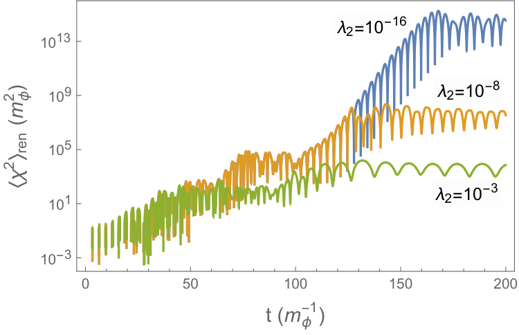
which determines how efficient parametric resonance is. Adding backreaction on the inflaton motion introduces yet another dimensionless parameter, $\lambda_{2}$, which controls how $\braket{\chi^{2}}$ impacts the inflaton motion. Although $\lambda_{2}$ and $q_{0}$ are related by equation (3.24), it is useful to regard them as independent parameters. The limit $\lambda_{2}\to 0$ while $q_{0}$ remains finite, in particular, is the limit in which there is no backreaction of matter on the inflaton motion. Figure 3 displays the dependence of $\braket{\chi^{2}}$ on the cutoff used in our numerical implementation in that limit: Panel (a) shows the unrenormalized value of $\braket{\chi^{2}}$, that is, the cut off integral in (3.7) computed numerically. Panel (b) shows its renormalized value, that is, the term in square brackets in equation (3.19). Clearly, the renormalized expectation on the right does not depend on $\Lambda$, as expected. In fact, provided that the cutoff $\Lambda$ is not chosen to be much larger than the magnitude of the modes expected to undergo parametric resonance, the subtraction terms needed to renormalize the expectation value play an important role only when $q_{0}$ is sufficiently small [13]. Figure 4 displays the dependence of $\braket{\chi^{2}}_{\mathrm{ren}}$ on the value of $q_{0}$ in the absence of backreaction, $\lambda_{2}\to 0$, and its dependence on $\lambda_{2}\neq 0$ when backreaction is taken into account. In the absence of backreaction the matter mode functions grow exponentially with $q_{0}$, and so does $\braket{\chi^{2}}_{\mathrm{ren}}$. This strong dependence, however, is quenched by backreaction, which, as shown on the right panel of figure 4, suppresses $\braket{\chi^{2}}_{\mathrm{ren}}$ as the coupling $\lambda_{2}$ increases. Because of equation (3.4b), backreaction on the inflaton motion ought to be relevant when $\lambda_{2}\braket{\chi^{2}}\gtrsim m_{\phi}^{2}$. This is why $\braket{\chi^{2}}_{\mathrm{ren}}$ stops growing once $\braket{\chi^{2}}_{\mathrm{ren}}/m_{\phi}^{2}$ becomes of the order of $\lambda_{2}^{-1}$.

The gravitational equations (4.1) are not all independent, since the Einstein and energy-momentum tensors are covariantly conserved. We shall hence restrict our attention to their time-time component, which we shall deem the “Friedman” equation

$$\frac{\mathcal{H}^{2}}{a^{2}}=\frac{a^{2}\braket{T^{00}}}{3M_{P}^{2}},\quad a^{2}\braket{T^{00}}\equiv\bar{\rho}_{\phi}+\rho_{\chi}.$$

(4.3)

This restriction also simplifies the role played by boundary terms, as we discuss in appendix D. The energy density of matter $\rho_{\chi}\equiv a^{2}\langle T^{00}_{(\chi)}\rangle$ can be expanded again in the number of time derivatives. In this case, to capture all the potentially divergent terms we need to go up to four derivatives,

	$\displaystyle\rho_{\chi}^{(0)}$	$\displaystyle=\frac{1}{8(2\pi^{2})}\sum_{i}\sigma_{i}\left[\frac{\Lambda^{4}}{a^{4}}+\frac{\kappa_{i}\Lambda^{2}}{a^{2}}+\frac{\kappa_{i}^{2}}{4}\left(\frac{1}{2}-\log x_{i}\right)\right],$		(4.4a)
	$\displaystyle\rho_{\chi}^{(2)}$	$\displaystyle=\frac{1}{8(2\pi^{2})}\sum_{i}\sigma_{i}\left[\frac{\Lambda^{2}\mathcal{H}^{2}}{a^{4}}-\frac{\kappa_{i}\mathcal{H}^{2}}{a^{2}}\left(\frac{4}{3}-\frac{1}{2}\log x_{i}\right)-\frac{\dot{\kappa}_{i}\mathcal{H}}{2a^{2}}\left(\frac{5}{3}-\log x_{i}\right)+\frac{\dot{\kappa}^{2}_{i}}{24a^{2}\kappa_{i}}\right],$		(4.4b)
	$\displaystyle\rho_{\chi}^{(4)}$	$\displaystyle=\frac{1}{8(2\pi^{2})}\sum_{i}\sigma_{i}\left[-\frac{\mathcal{H}^{4}}{60a^{4}}-\frac{4\mathcal{H}^{2}\ddot{a}}{15a^{5}}-\frac{19\ddot{a}^{2}}{60a^{6}}+\frac{19\mathcal{H}\dddot{a}}{30a^{5}}+\left(\frac{\mathcal{H}^{2}\ddot{a}}{a^{5}}+\frac{1}{4}\frac{\ddot{a}^{2}}{a^{6}}-\frac{1}{2}\frac{\mathcal{H}\dddot{a}}{a^{5}}\right)\log x_{i}\right],$		(4.4c)

where we have dropped terms of order $1/\Lambda$, and in (4.4c) also those that vanish in the limit $\kappa_{i}\to\infty$. These densities are finite as the cutoff $\Lambda$ approaches infinity, if in addition to conditions (3.11), the regulator masses satisfy

$$\sum_{i}\sigma_{i}M_{i}^{4}=0.$$

(4.5)

Although the expressions in (4.4) remain finite as the cutoff is removed, they depend on the regulator masses, and hence diverge when the regulators are decoupled. But these surviving contributions are of the same form as those from the additional counterterms

$$S_{\mathrm{ct}}\supset\int d^{4}x\sqrt{-g}\left[-\delta\Lambda+\frac{\delta M_{P}^{2}}{2}R+\delta c_{(1)}R^{2}+\delta c_{(2)}R_{\mu\nu}R^{\mu\nu}\right],$$

(4.6)

which renormalize the different terms in the Friedman equation (4.3). Let us cast the latter in the form

$$3M_{P}^{2}(\bar{\phi})H^{2}+\cdots=U(\bar{\phi})+\frac{1}{2a^{2}}\dot{\bar{\phi}}^{2}+\cdots,$$

(4.7)

where the dots stand for terms with higher derivatives of the scalar or the metric. At tree level we know that $U(\bar{\phi})=\bar{V}$, but at one loop the quantum corrections in (4.4a) modify this expression. We cancel the divergent $\bar{\phi}$-independent vacuum energy piece in $U$ by choosing

$$2\pi^{2}\delta\Lambda=\frac{1}{32}\sum_{r}\sigma_{r}M_{r}^{4}\log X_{r}+\delta\Lambda^{f}.$$

(4.8)

The dependence of $\delta\Lambda$ on the fourth power of the regulator masses is an expression of the cosmological constant problem. Because of relation (3.8), equation (4.4a) also yields regulator-dependent contributions to $U(\bar{\phi})$ proportional to $\bar{\lambda}$ and $\bar{\lambda}^{2}$. These are canceled precisely by the counterterms proportional to $\delta d_{1}$ and $\delta d_{2}$ in equations (3.14). Therefore the renormalized potential density is

$$\bar{U}_{\mathrm{ren}}=\bar{V}+\frac{1}{2\pi^{2}}\left[\frac{(M_{0}^{2}+\bar{\lambda})^{2}}{32}\log\frac{M_{0}^{2}+\bar{\lambda}}{M_{0}^{2}+\lambda(\mu)}+\delta\Lambda^{f}+\left(\delta d^{f}_{1}-\frac{M_{0}^{2}}{32}\right)\bar{\lambda}+\left(\delta d^{f}_{2}-\frac{3}{64}\right)\bar{\lambda}^{2}\right].$$

(4.9)

This result illustrates the importance of identifying the counterterms in the theory. If we simply subtract from the different expectation values their cutoff dependent contributions, there is no guarantee that the undetermined finite pieces in the potential density will be consistent with those of the driving term. In fact, in spite of their different origin, at zero derivatives both are related by

$$\left\langle\frac{\partial V}{\partial\phi}\right\rangle^{(0)}_{\mathrm{ren}}=\frac{d\bar{U}_{\mathrm{ren}}}{d\bar{\phi}}.$$

(4.10)

This property also holds for the regularized but unrenormalized forms of the driving term and the energy density, and trivially applies to the contribution of the counterterms.

The surviving summands proportional to $\mathcal{H}^{2}$ in equation (4.4b) are proportional to the left-hand-side of the Friedman equation (4.7), and thus renormalize the value of the Planck mass. In order to keep the Planck mass finite, the counterterm $\delta M_{P}^{2}$ needs to be

$$2\pi^{2}\delta M_{P}^{2}=\frac{1}{48}\sum_{r}\sigma_{r}M_{r}^{2}\log X_{r}+(\delta M_{P}^{2})^{f}.$$

(4.11)

Because $\kappa_{i}$ in equation (4.4b) depends on the inflaton, there is also a $\bar{\phi}$-dependent divergent renormalization of Planck’s mass, which is cancelled by the counterterm proportional to $\delta\xi$ in (3.14c). As a result, the renormalized, inflaton-dependent Planck mass in the effective Friedman equation is

$$M_{P}^{2}(\bar{\phi})=M_{P}^{2}+\frac{1}{2\pi^{2}}\left\{(\delta M_{P}^{2})^{f}-2\delta\xi^{f}\bar{\lambda}+\frac{1}{48}\left[(M_{0}^{2}+\bar{\lambda})\log\frac{M_{0}^{2}+\bar{\lambda}}{M_{0}^{2}+\lambda(\mu)}-\bar{\lambda}\right]\right\},$$

(4.12)

which shows that the Planck mass “runs” with the inflaton value. Equation (4.4b) also contains terms proportional to $\mathcal{H}\dot{\kappa}_{i}=\mathcal{H}\dot{\bar{\lambda}}$. Their divergent contribution cancels the one we obtain by varying the $\delta\xi$ counterterm in equation (3.12), provided that $\delta\xi$ is still given by equation (3.14c). There is however a left-over finite piece that can be thought of as the renormalized value of the energy density at two derivatives,

$$\left(\delta\rho_{\chi}^{(2)}\right)_{\mathrm{ren}}=\frac{1}{2\pi^{2}}\left[6\delta\xi^{f}-\frac{1}{16}\log\frac{M_{0}^{2}+\bar{\lambda}}{M_{0}^{2}+\lambda(\mu)}\right]\frac{\mathcal{H}\dot{\bar{\lambda}}}{a^{2}}.$$

(4.13)

In order to determine the values of the counterterms proportional to $\delta c_{(1)}$ and $\delta c_{(2)}$ in equation (4.6) we need to find out how they contribute to the gravitational equations. Their variation with respect to the metric yields the tensors usually labeled ${}^{(1)}\!H_{\mu\nu}$ and ${}^{(2)}\!H_{\mu\nu}$ respectively. A relatively direct route to easily compute their $00$ components is to substitute the ADM metric ${ds^{2}=-N^{2}dt^{2}+a^{2}(t)d\vec{x}\,^{2}}$ into the action (4.6), vary with respect to the lapse function $N$, and then choose a gauge with $N=a$. The result is

	$\displaystyle\frac{1}{\mathcal{V}}\frac{\delta}{\delta N}\left(\int d^{4}x\sqrt{-g}\,R^{2}\right)$	$\displaystyle=-144\frac{\dot{a}^{2}\ddot{a}}{a^{4}}-36\frac{\ddot{a}^{2}}{a^{3}}+72\frac{\dot{a}\,\dddot{a}}{a^{3}},$		(4.14a)
	$\displaystyle\frac{1}{\mathcal{V}}\frac{\delta}{\delta N}\left(\int d^{4}x\sqrt{-g}\,R_{\mu\nu}R^{\mu\nu}\right)$	$\displaystyle=-48\frac{\dot{a}^{2}\ddot{a}}{a^{4}}-12\frac{\ddot{a}^{2}}{a^{3}}+24\frac{\dot{a}\,\dddot{a}}{a^{3}},$		(4.14b)

where we have ignored boundary terms, which we discuss in appendix D. The two variations are proportional to each other, owing to the fact that in a conformally flat spacetime ${}^{(1)}\!H_{ab}=3\times\!{}^{(2)}\!H_{ab}$. The log divergent piece in $\langle\rho_{\chi}\rangle^{(4)}$ is also proportional to either variation. Therefore, by demanding the cancellation of this divergence, we can only fix a linear combination of $\delta c_{(1)}$ and $\delta c_{(2)}$,

$$2\pi^{2}(3\delta c_{(1)}+\delta c_{(2)})=-\frac{1}{384}\sum_{r}\sigma_{r}\log X_{r}+\delta c^{f}.$$

(4.15)

To disentangle the two individual contributions we would have to consider more general backgrounds. In any case, the renormalized energy density at four derivatives thus becomes

$$\delta\rho_{\chi}^{(4)}=\frac{1}{2\pi^{2}}\left[48\,\delta c^{f}-\frac{1}{8}\log\frac{M_{0}^{2}+\bar{\lambda}}{M_{0}^{2}+\lambda(\mu)}\right]\left(\frac{\mathcal{H}^{2}\ddot{a}}{a^{5}}+\frac{1}{4}\frac{\ddot{a}^{2}}{a^{6}}-\frac{1}{2}\frac{\mathcal{H}\dddot{a}}{a^{5}}\right).$$

(4.16)

Finally, with the counterterms given by the previous expressions, the one-loop “exact” renormalized value of the energy density reads

	$$\begin{split}\braket{\rho_{\chi}}_{\mathrm{ren}}&=\frac{1}{2\pi^{2}}\Bigg\{\frac{1}{2a^{2}}\lim_{\Lambda\to\infty}\int_{0}^{\Lambda}dk\,k^{2}\left[\dot{w}_{k}\dot{w}^{*}_{k}+(k^{2}+\kappa_{0}a^{2})w_{k}w^{*}_{k}\right]\\ &-\frac{\Lambda^{4}}{8a^{4}}-\frac{\kappa_{0}\Lambda^{2}}{8a^{2}}+\frac{\kappa_{0}^{2}}{32}\log\frac{4\Lambda^{2}}{a^{2}\kappa_{\mu}}+f_{0}\\ &-\frac{\Lambda^{2}\mathcal{H}^{2}}{8a^{4}}-\frac{\kappa_{0}\mathcal{H}^{2}}{16a^{2}}\log\frac{4\Lambda^{2}}{a^{2}\kappa_{\mu}}-\frac{\dot{\bar{\lambda}}\mathcal{H}}{16a^{2}}\log\frac{4\Lambda^{2}}{a^{2}\kappa_{\mu}}+f_{2}\\ &-\frac{1}{8}\left(\frac{\mathcal{H}^{2}\ddot{a}}{a^{5}}+\frac{1}{4}\frac{\ddot{a}^{2}}{a^{6}}-\frac{1}{2}\frac{\mathcal{H}\dddot{a}}{a^{5}}\right)\log\frac{4\Lambda^{2}}{a^{2}\kappa_{\mu}}+f_{4}\Bigg\},\end{split}$$				(4.17a)
where the remaining cutoff independent finite contributions are
	$\displaystyle f_{0}$	$\displaystyle\equiv$	$\displaystyle\delta\Lambda^{f}-\frac{M_{0}^{4}}{64}+\left(\delta d_{1}^{f}-\frac{M_{0}^{2}}{16}\right)\bar{\lambda}+\left(\delta d_{2}^{f}-\frac{1}{16}\right)\bar{\lambda}^{2},$		(4.17b)
	$\displaystyle f_{2}$	$\displaystyle\equiv$	$\displaystyle\frac{\mathcal{H}^{2}}{a^{2}}\left[\frac{M_{0}^{2}}{6}-3(\delta M_{P}^{2})^{f}+\left(\frac{11}{48}+6\delta\xi^{f}\right)\bar{\lambda}\right]+\frac{\mathcal{H}\dot{\bar{\lambda}}}{a^{2}}\left[6\delta\xi^{f}+\frac{5}{48}\right],$		(4.17c)
	$\displaystyle f_{4}$	$\displaystyle\equiv$	$\displaystyle\frac{\mathcal{H}^{4}}{480a^{4}}+\frac{\mathcal{H}^{2}\ddot{a}}{30a^{5}}+\frac{19\ddot{a}^{2}}{480a^{6}}-\frac{19\mathcal{H}\dddot{a}}{240a^{5}}+48\delta c^{f}\left(\frac{\mathcal{H}^{2}\ddot{a}}{a^{5}}+\frac{1}{4}\frac{\ddot{a}^{2}}{a^{6}}-\frac{1}{2}\frac{\mathcal{H}\dddot{a}}{a^{5}}\right).$		(4.17d)

We compute the renormalized matter pressure along the same lines in appendix A.

It can be checked explicitly that (4.17) yields the renormalized expressions that we have derived above. Although the regulators play no role in this final expression, the renormalized energy density does not simply follow from removing the cutoff dependence from the mode integral. Our regularization scheme forces us to subtract a term proportional to $\mathcal{H}^{4}/a^{4}$, but the latter does not appear in any of the log-divergent terms. In addition, the finite pieces at any number of derivatives do not have the same structure as the corresponding log-divergent terms. This again underscores the importance of a complete analysis of regularization and renormalization. Removing the cutoff-dependent contributions by hand, or simply isolating the logarithmic divergences is not sufficient.

The reader may have recognized in equation (4.17) an expression akin to the renormalized energy-momentum tensor in the adiabatic scheme. This is because in the latter one subtracts from the divergent expectation an expansion of the same quantity in the number of time derivatives, up to the number that renders the expression finite (four in the case of $T^{\mu\nu}$). Apart from terms that vanish when $\kappa_{i}\to\infty$, and we did not write down, this expansion is precisely the one contained in equations (4.4) when restricted just to the $i=0$ contribution. This also happens to be essentially what we subtract in the renormalized expression (4.17). Thus, the main differences between the adiabatic scheme and Pauli-Villars are that $i)$ expression (4.17) also contains the explicit contributions from the counterterms needed to enforce the renormalization conditions, $ii)$ in the adiabatic scheme one would presumably subtract $\phi$-dependent logarithms, $\log\kappa_{0}$ instead of the $\log\kappa_{\mu}$ in (4.17), $iii)$ we are not subtracting any of the time derivatives of $\bar{\phi}$ that arise from the dependence of the effective square mass $\kappa_{0}$ on the inflaton $\bar{\phi}$. These differences are inconsequential for free fields, but are significant when their mass depends on an external field like $\bar{\phi}$. In the former case, our derivation can be thought of as further justification for the standard adiabatic scheme. In general however, we feel that Pauli-Villars is a superior regularization scheme. To our knowledge, its use in cosmology was first advocated for by S. Weinberg in reference [24].

The higher-curvature corrections needed to renormalize the theory in equation (4.17) should be appropriately interpreted. In this work we regard general relativity as a low-energy effective field theory, and, as such, the renormalized contributions of the counterterms are only supposed to capture corrections to the equations of motion derived at lowest order, that is, in general relativity.

The higher time derivatives present in the corrected Friedman equation (4.3), however, suggest otherwise. They not only imply that the order of this differential equation changes, which amounts to a change in the number of degrees of freedom in the theory, but also lead to solutions that cannot be thought of as corrections to the lowest order theory. An illuminating example is that of Starobinsky inflation [25], in which a literal solution of the equations of motion in the presence of an $R^{2}$ term yields inflating solutions that are altogether absent in general relativity [26].

An appropriate way to deal with higher derivative corrections from the point of view of effective field theory has been lucidly discussed by J. Z. Simon in [27]. In practice, it implies that we can use the “tree-level” Friedman equation to reduce the order of the quantum-corrected equation (4.3), as explicitly discussed in [28]. This procedure almost guarantees that the solutions of the reduced equations display the desired property of being low-energy expansions grounded on the lowest order approximation of general relativity.

Reference [28] carried out such an order reduction in a universe dominated by radiation, but not in the case of a scalar-field dominated universe that occupies us. To reduce the order of the “Friedman” equation (4.3) in that case we shall simply use the $i$-$j$ Einstein equation

$$\frac{\ddot{a}}{a^{3}}=\frac{1}{6M_{P}^{2}}\left(-\dot{\bar{\phi}}^{2}+4\bar{V}a^{2}\right)$$

(4.18)

and its time derivative to replace $\ddot{a}$ and $\dddot{a}$ in equation (4.17) by expressions with a lower number of derivatives. This procedure leaves factors of $\ddot{\bar{\phi}}$, which we eliminate using the inflaton equation of motion. The outcome is that the last line in equation (4.17) should be replaced by

$$\begin{split}\frac{\mathcal{H}^{4}}{480a^{4}}&-\frac{\mathcal{H}^{2}(196a^{2}V+65\dot{\phi}^{2})}{1440M_{P}^{2}a^{4}}-\frac{19\mathcal{H}\bar{V}^{\prime}\bar{\phi}^{\prime}}{240M_{P}^{2}a^{2}}+\frac{19(\dot{\bar{\phi}}^{2})^{2}-4a^{2}\bar{V}}{17280M_{P}^{4}a^{4}}\\ &+\left(48\delta c^{f}-\frac{1}{8}\log\frac{4\Lambda^{2}}{a^{2}\kappa_{\mu}}\right)\left[\frac{(\dot{\bar{\phi}}^{2}-4a^{2}\bar{V})^{2}}{144M_{P}^{4}a^{4}}-\frac{\mathcal{H}\bar{V}^{\prime}\dot{\bar{\phi}}}{2M_{P}^{2}a^{2}}-\frac{\mathcal{H}^{2}(5\dot{\phi}^{2}+4a^{2}V)}{12M_{P}^{2}a^{4}}\right],\end{split}$$

(4.19)

which manifestly preserves the differential order of the original Friedman equation.

These considerations also affect the evaluation of the renormalized energy density (4.17). In that equation, $\mathcal{H}$ refers to the expansion rate at the corresponding time $t$, which is putatively constrained by equation (4.3). But since $\braket{\rho_{\chi}}_{\mathrm{ren}}$ captures the lowest-order correction in the effective field theory expansion, $\mathcal{H}$ in equation (4.17) ought to be evaluated using the zeroth order Friedman equation $3M_{P}^{2}\mathcal{H}^{2}=a^{2}\bar{\rho}_{\phi}$.

Our numerical solutions also include backreaction on the expansion of the universe. For illustration, we shall return again to the specific quadratic potential and coupling function (3.21), with the finite values of the counterterms given by equation (3.23). To fix the value of the remaining counterterms we set $\delta c^{f}=0$ and demand that $M_{P}^{2}(\mu)=M_{P}^{2}$ and $U_{\mathrm{ren}}(\bar{\phi}=0)=0$, which imply that

$$\delta\Lambda^{f}=0,\quad(\delta M_{P}^{2})^{f}=0.$$

(4.20)

As detailed in appendix C, in this case the impact of backreaction on the metric is controlled by the dimensionless ratio

$$r\equiv\frac{m_{\phi}^{2}}{M_{P}^{2}}=\frac{2\lambda_{2}}{3q_{0}}$$

(4.21)

which, in spite of its relation to $\lambda_{2}$ and $q_{0}$, we regard as an independent parameter in our numerical code. In the limit $r\to 0$ metric backreaction is turned off, whereas as $r$ grows it becomes increasingly important.

Figure 6 shows the dependence of both the unrenormalized and renormalized matter energy density for different values of the cutoff in the absence of backreaction, both on the inflaton and on the expansion. The independence of the renormalized expectation on the value of the cutoff is a powerful check not only of our renormalization procedure, but also on the numerical algorithm itself. Note in particular that the renormalization of $\braket{\rho_{\chi}}$ requires the subtraction of a term of order $\Lambda^{4}$, whereas that of $\braket{\chi^{2}}$ only requires the subtraction of a term of order $\Lambda^{2}$. The dependence of $\braket{\rho_{\chi}}_{\mathrm{ren}}$ on $q_{0}$ and $\lambda_{2}$ is explored in figure 7. Parametric resonance is only effective during the first oscillations of the inflaton, and ceases to be effective after a time proportional to $\sqrt{q_{0}}$ [2]. Panel (a) of figure 7 also shows how the energy density of matter redshifts after parametric resonance becomes ineffective. The $x^{-8/3}$ decay indicates that the latter behaves as radiation, as expected from our choice $M_{0}=0$.²² 2 As the inflaton oscillates about its minimum, the scale factor grows as in a matter-dominated universe, $a\propto x^{2/3}$, where $x=m_{\phi}\tau$ is cosmic time in units of the inverse inflaton mass. Therefore radiation is expected to redshift like $a^{-4}\propto x^{-8/3}$.

The effects of backreaction on the inflaton motion are illustrated in figure 8. The evolution of the inflaton is seen to depart from the one in the absence of backreaction precisely around the time the density of matter reaches its maximum (see panel (b) in figure 7.) We interpret this departure as the decay of the inflaton into radiation. The inflaton density subsequently shows a strong oscillatory behavior with an average value that steadily decreases. To determine the effective equation of state of the inflaton during such period, we plot the scale factor as a function of time in panel (b) with the parameter $r$ set to zero (matter fields then have no impact on the universe expansion.) There is a sharp break in the evolution of $a$, from matter-dominated expansion to that associated with an effective equation of state “stiffer” than that of radiation, $w_{\phi}\approx 2/3$. The latter suggests that radiation can come to dominate the universe.

Because cosmic expansion is dictated by the total energy density, a simple way to determine whether backreaction on cosmic expansion is relevant is to compare the energy density of matter with that of the inflaton. In fact, $\braket{\rho_{\chi}}_{\mathrm{ren}}$ needs to surpass $\bar{\rho}_{\phi}$ for reheating to be successful. In terms of the relevant dimensionless ratio, this condition becomes

$$\frac{m_{\phi}^{2}}{M_{P}^{2}}\frac{\braket{\rho_{\chi}}_{\mathrm{ren}}}{m_{\phi}^{4}}\gtrsim\frac{\bar{\rho}_{\phi}}{m_{\phi}^{2}M_{P}^{2}}.$$

(4.22)

Since it is reasonable to assume that $m_{\phi}<M_{P}$, a necessary condition for backreaction to play a role is that $\braket{\rho_{\chi}}_{\mathrm{ren}}/m_{\phi}^{4}$ grow larger than $\bar{\rho}_{\phi}/(m_{\phi}^{2}M_{P}^{2})$. This stronger condition is useful because the two dimensionless ratios can be estimated with the value of $q_{0}$ alone. Our numerical analysis indeed indicates that $\braket{\rho_{\chi}}_{\mathrm{ren}}/m_{\phi}^{4}$ can become larger than $\bar{\rho}_{\phi}/(m_{\phi}^{2}M_{P}^{2})$ only if $q_{0}\gtrsim 25$. Thus, within our approximations, it appears that a successful reheating is not possible for smaller values of $q_{0}$. This conclusion also agrees with the results of the perturbative analysis of, say, reference [2]. Equation (4.21) may suggest that an increase in $q_{0}$ makes backreaction less important, but, in fact, because the matter density grows exponentially with $q_{0}$, the opposite is true. Yet successful reheating also demands that the matter density remain above that of the inflaton. After its initial growth during the initial stages of preheating, the matter density begins to redshift like radiation, whereas in the absence of backreaction that of the inflaton redshifts like non-relativistic matter. It is then important that backreaction on the inflaton motion, which is controlled by the parameter $\lambda_{2}$, be large enough to affect its evolution. Since $\lambda_{2}$ appears in combination with $\braket{\rho_{\chi}}_{\mathrm{ren}}$, and the later grows exponentially with $q_{0}$, it typically suffices that $\lambda_{2}$ not be too small. As we mentioned earlier, when backreaction on the inflaton motion is relevant, its energy density decays faster than radiation, as required by a successful reheating.

References

- [1] B. P. Abbott et al. [LIGO Scientific and Virgo Collaborations], “Observation of Gravitational Waves from a Binary Black Hole Merger,” Phys. Rev. Lett. 116, no. 6, 061102 (2016) doi:10.1103/PhysRevLett.116.061102 [arXiv:1602.03837 [gr-qc]].
- [2] L. Kofman, A. D. Linde and A. A. Starobinsky, “Towards the theory of reheating after inflation,” Phys. Rev. D 56, 3258 (1997) doi:10.1103/PhysRevD.56.3258 [hep-ph/9704452].
- [3] R. Allahverdi, R. Brandenberger, F. Y. Cyr-Racine and A. Mazumdar, “Reheating in Inflationary Cosmology: Theory and Applications,” Ann. Rev. Nucl. Part. Sci. 60, 27 (2010) doi:10.1146/annurev.nucl.012809.104511 [arXiv:1001.2600 [hep-th]].
- [4] M. A. Amin, M. P. Hertzberg, D. I. Kaiser and J. Karouby, “Nonperturbative Dynamics Of Reheating After Inflation: A Review,” Int. J. Mod. Phys. D 24, 1530003 (2014) doi:10.1142/S0218271815300037 [arXiv:1410.3808 [hep-ph]].
- [5] G. N. Felder and I. Tkachev, “LATTICEEASY: A Program for lattice simulations of scalar fields in an expanding universe,” Comput. Phys. Commun. 178, 929 (2008) doi:10.1016/j.cpc.2008.02.009 [hep-ph/0011159].
- [6] A. V. Frolov, “DEFROST: A New Code for Simulating Preheating after Inflation,” JCAP 0811, 009 (2008) doi:10.1088/1475-7516/2008/11/009 [arXiv:0809.4904 [hep-ph]].
- [7] J. Sainio, “CUDAEASY - a GPU Accelerated Cosmological Lattice Program,” Comput. Phys. Commun. 181, 906-912 (2010) doi:10.1016/j.cpc.2010.01.002 [arXiv:0911.5692 [astro-ph.IM]].
- [8] R. Easther, H. Finkel and N. Roth, “PSpectRe: A Pseudo-Spectral Code for (P)reheating,” JCAP 1010, 025 (2010) doi:10.1088/1475-7516/2010/10/025 [arXiv:1005.1921 [astro-ph.CO]].
- [9] Z. Huang, “The Art of Lattice and Gravity Waves from Preheating,” Phys. Rev. D 83, 123509 (2011) doi:10.1103/PhysRevD.83.123509 [arXiv:1102.0227 [astro-ph.CO]].
- [10] H. L. Child, J. T. Giblin, Jr, R. H. Ribeiro and D. Seery, “Preheating with Non-Minimal Kinetic Terms,” Phys. Rev. Lett. 111, 051301 (2013) doi:10.1103/PhysRevLett.111.051301 [arXiv:1305.0561 [astro-ph.CO]].
- [11] K. D. Lozanov and M. A. Amin, “GFiRe: a Gauge Field integrator for Reheating,” arXiv:1911.06827 [astro-ph.CO].
- [12] S. Y. Khlebnikov and I. I. Tkachev, “Relic gravitational waves produced after preheating,” Phys. Rev. D 56, 653 (1997) doi:10.1103/PhysRevD.56.653 [hep-ph/9701423].
- [13] C. Armendariz-Picon, “On the Expected Production of Gravitational Waves During Preheating,” JCAP 1908, 012 (2019) doi:10.1088/1475-7516/2019/08/012 [arXiv:1905.05724 [astro-ph.CO]].
- [14] S. Weinberg, “Quantum contributions to cosmological correlations,” Phys. Rev. D 72, 043514 (2005) doi:10.1103/PhysRevD.72.043514 [hep-th/0506236].
- [15] D. Green and R. A. Porto, “Signals of a Quantum Universe,” arXiv:2001.09149 [hep-th].
- [16] E. Calzetta and B. L. Hu, “Closed Time Path Functional Formalism in Curved Space-Time: Application to Cosmological Back Reaction Problems,” Phys. Rev. D 35, 495 (1987). doi:10.1103/PhysRevD.35.495.
- [17] L. R. W. Abramo, R. H. Brandenberger and V. F. Mukhanov, “The Energy - momentum tensor for cosmological perturbations,” Phys. Rev. D 56, 3248 (1997) doi:10.1103/PhysRevD.56.3248 [gr-qc/9704037].
- [18] T. S. Koivisto and T. Prokopec, “Quantum backreaction in evolving FLRW spacetimes,” Phys. Rev. D 83, 044015 (2011) doi:10.1103/PhysRevD.83.044015 [arXiv:1009.5510 [gr-qc]].
- [19] T. Markkanen and A. Tranberg, “Quantum Corrections to Inflaton and Curvaton Dynamics,” JCAP 1211, 027 (2012) doi:10.1088/1475-7516/2012/11/027 [arXiv:1207.2179 [gr-qc]].
- [20] P. B. Greene and L. Kofman, “Preheating of fermions,” Phys. Lett. B 448, 6 (1999) doi:10.1016/S0370-2693(99)00020-9 [hep-ph/9807339].
- [21] C. Armendariz-Picon, “When Does the Inflaton Decay?,” JCAP 1805, 018 (2018) doi:10.1088/1475-7516/2018/05/018 [arXiv:1708.09755 [hep-th]].
- [22] S. Weinberg, “Perturbative Calculations of Symmetry Breaking,” Phys. Rev. D 7, 2887-2910 (1973) doi:10.1103/PhysRevD.7.2887
- [23] S. R. Coleman and E. J. Weinberg, “Radiative Corrections as the Origin of Spontaneous Symmetry Breaking,” Phys. Rev. D 7, 1888 (1973). doi:10.1103/PhysRevD.7.1888
- [24] S. Weinberg, “Ultraviolet Divergences in Cosmological Correlations,” Phys. Rev. D 83, 063508 (2011) doi:10.1103/PhysRevD.83.063508 [arXiv:1011.1630 [hep-th]].
- [25] A. A. Starobinsky, “A New Type of Isotropic Cosmological Models Without Singularity,” Phys. Lett. 91B, 99 (1980) [Adv. Ser. Astrophys. Cosmol. 3, 130 (1987)].
- [26] J. Z. Simon, “No Starobinsky inflation from selfconsistent semiclassical gravity,” Phys. Rev. D 45, 1953 (1992). doi:10.1103/PhysRevD.45.1953
- [27] J. Z. Simon, “Higher Derivative Lagrangians, Nonlocality, Problems and Solutions,” Phys. Rev. D 41, 3720 (1990). doi:10.1103/PhysRevD.41.3720
- [28] L. Parker and J. Z. Simon, “Einstein equation with quantum corrections reduced to second order,” Phys. Rev. D 47, 1339 (1993) doi:10.1103/PhysRevD.47.1339 [gr-qc/9211002].
- [29] Y. Akrami et al. [Planck Collaboration], “Planck 2018 results. X. Constraints on inflation,” arXiv:1807.06211 [astro-ph.CO].
- [30] C. J. Moore, R. H. Cole and C. P. L. Berry, “Gravitational-wave sensitivity curves,” Class. Quant. Grav. 32, no. 1, 015014 (2015) doi:10.1088/0264-9381/32/1/015014 [arXiv:1408.0740 [gr-qc]].
- [31] B. P. Abbott et al. [LIGO Scientific Collaboration], “Exploring the Sensitivity of Next Generation Gravitational Wave Detectors,” Class. Quant. Grav. 34, no. 4, 044001 (2017) doi:10.1088/1361-6382/aa51f4 [arXiv:1607.08697 [astro-ph.IM]].
- [32] R. L. Arnowitt, S. Deser and C. W. Misner, “The Dynamics of general relativity,” Gen. Rel. Grav. 40, 1997 (2008) doi:10.1007/s10714-008-0661-1 [gr-qc/0405109].
- [33] J. W. York, Jr., “Role of conformal three geometry in the dynamics of gravitation,” Phys. Rev. Lett. 28, 1082 (1972). doi:10.1103/PhysRevLett.28.1082
- [34] G. W. Gibbons and S. W. Hawking, “Action Integrals and Partition Functions in Quantum Gravity,” Phys. Rev. D 15, 2752 (1977). doi:10.1103/PhysRevD.15.2752
- [35] A. D. Barvinsky and S. N. Solodukhin, “Nonminimal coupling, boundary terms and renormalization of the Einstein-Hilbert action and black hole entropy,” Nucl. Phys. B 479, 305 (1996) doi:10.1016/0550-3213(96)00438-5 [gr-qc/9512047].
- [36] G. ’t Hooft and M. J. G. Veltman, “One loop divergencies in the theory of gravitation,” Ann. Inst. H. Poincare Phys. Theor. A 20, 69 (1974).
- [37] N. Deruelle, N. Merino and R. Olea, “Einstein-Gauss-Bonnet theory of gravity: The Gauss-Bonnet-Katz boundary term,” Phys. Rev. D 97, no. 10, 104009 (2018) doi:10.1103/PhysRevD.97.104009 [arXiv:1709.06478 [gr-qc]].
- [38] E. Dyer and K. Hinterbichler, “Boundary Terms, Variational Principles and Higher Derivative Modified Gravity,” Phys. Rev. D 79, 024028 (2009) doi:10.1103/PhysRevD.79.024028 [arXiv:0809.4033 [gr-qc]].
- [39] M. S. Madsen and J. D. Barrow, “De Sitter Ground States and Boundary Terms in Generalized Gravity,” Nucl. Phys. B 323, 242 (1989). doi:10.1016/0550-3213(89)90596-8