Chemical reaction network decompositions and realizations of S-systems
Abstract
This paper presents novel decomposition classes of chemical reaction networks (CRNs) derived from S-system kinetics. Based on the network decomposition theory initiated by Feinberg in 1987, we introduce the concept of incidence independent decompositions and develop the theory of - and - decompositions which partition the set of complexes and the set of nonzero complexes respectively, including their structure theorems in terms of linkage classes. Analogous to Feinberg’s independent decomposition, we demonstrate the important relationship between sets of complex balance equilibria for an incidence independent decomposition of weakly reversible subnetworks for any kinetics. We show that the -decompositions are also incidence independent. We also introduce in this paper a new realization for an S-system that is analyzed using a newly defined class of species coverable CRNs. This led to the extension of the deficiency formula and characterization of fundamental decompositions of species decomposable reaction networks.
Keywords: Chemical reaction network theory, S-system, network decomposition, subnetwork realization, species coverable CRNs, species decomposable CRN
1 Introduction
S-systems consist of ordinary differential equations (ODEs) of the form
where are nonnegative and the exponents are arbitrary real numbers. For convenience, we assume that the variables are restricted to positive real values. They form a special class of power law dynamical systems, which are called Generalized Mass Action (GMA) systems in Biochemical Systems Theory (BST). -systems were introduced in M. Savageau’s seminal work in 1969 [21, 22, 26] and have been extensively applied in modeling complex biochemical systems in many fields, see e.g. Voit’s review [27]. Various authors have studied chemical kinetic systems (CKS) which are realizations, i.e. dynamically equivalent or have the identical set of ODEs as the dynamical system [16, 19, 20, 1, 2].
This paper presents novel concepts and results on decompositions of chemical reaction networks (CRN) that we derived from
- •
- •
the study of kinetic system realizations of -systems which are dominant subsystems of GMA systems in design space theory [23].
In the first part of the paper, we introduce the concept of incidence independent decompositions of a CRN, which complements the independence property defined by M. Feinberg in 1987 [9]. A basic property of an incidence independent decomposition is the inequality: , where and denote the deficiency of the network and the subnetwork respectively.
We identify the important subset of -decompositions, which are those generated by partitions of the reaction set which are also partitions of the set of complexes. The best known example of a -decomposition is the set of linkage classes of a CRN. We provide a characterization of -decompositions in terms of linkage classes.
Feinberg demonstrated the importance of independent decompositions by stating the relationship of the sets of positive equilibria of the network and those of the subnetworks for any kinetics. We derive the analogous result for incidence independent decompositions of weakly reversible subnetworks and the sets of complex balanced equilibria. We conclude the first part with the study of -decompositions, which partition the nonzero complexes of the network and show that these are also incidence independent.
In the second part of the paper, we introduce a new realization for an -system, which we call the subnetwork realization. This concept is motivated by studies of design spaces, where -subsystems of a GMA system are used to analyze the system’s behavior. To analyze the subnetwork realization and its predecessor, now called the independent realization of an -system, we introduce the class of species coverable CRNs. We then extend the deficiency formula of Arceo et al. [1] and the characterization of fundamental decompositions by Hernandez et al. [15] for the independent realization of an -system to any species decomposable CRN.
The main new results of the paper are:
- •
the characterization of the structure of -decompositions (Theorem 1);
- •
- •
the characterization of the structure of -decompositions (Theorem 6) and its corollary (incidence independence of -decompositions); and
- •
the extensions of the deficiency formula and characterization of fundamental decompositions to species decomposable reaction networks (Theorem 7).
The paper is organized as follows: Section 2 collects the fundamental concepts and results on CRNs and kinetic systems needed in the latter sections. The result on incidence independent decompositions, -decompositions and -decompositions are derived and discussed in Section 3. Section 4 introduces the realizations of -systems, species coverable and species decomposable CRNs. The final section provides a summary and outlook.
2 Fundamentals of chemical reaction networks and kinetic systems
We recall the necessary concepts of chemical reaction networks and the mathematical notations used throughout the paper adopted from the papers [1], [9] and [13].
We begin with the definition of a chemical reaction network.
Definition 1.
A chemical reaction network is a triple of three non-empty finite sets:
- 1.
A set of species ,
- 2.
A set of complexes, which are non-negative integer linear combinations of the species, and
- 3.
A set of reactions such that
- •
for all , and
- •
for each , there exists a such that or
- •
Two useful maps are associated with each reaction:
Definition 2.
The reactant map maps a reaction to its reactant complex while the product map maps it to its product complex. We denote with , i.e., the number of reactant complexes.
Connectivity concepts in Digraph Theory apply to CRNs, but have slightly differing names. A connected component is traditionally called a linkage class, denoted by , in CRNT. A subset of a linkage class where any two elements are connected by a directed path in each direction is known as a strong linkage class. If there is no reaction from a complex in the strong linkage class to a complex outside the same strong linkage class, then we have a terminal strong linkage class. We denote the number of linkage classes with , that of the strong linkage classes with and that of terminal strong linkage classes with . Clearly, A CRN is said to be weakly reversible if , and it is said to be -minimal if .
Many features of CRNs can be examined by working in terms of finite dimensional spaces which are referred to as species space, complex space and reaction space, respectively. We can view a complex as a vector in (called complex vector) by writing where is the stoichiometric coefficient of species .
Definition 3.
The reaction vectors of a CRN are the members of the set The stoichiometric subspace of the CRN is the linear subspace of defined by
The rank of the CRN, , is defined as
Definition 4.
The incidence map is defined as follows. For , then and if and , respectively, and are otherwise.
Equivalently, it maps the basis vector to if .
It is clearly a linear map, and its matrix representation (with respect to the standard bases , ) is called the incidence matrix, which can be described as
Note that in most digraph theory books, the incidence matrix is set as .
An important result of digraph theory regarding the incidence matrix is the following:
Proposition 1.
Let be a CRN. Denote by the incidence matrix of the directed graph . Then rank , where is the number of complexes and is the number of linkage classes of a CRN.
A non-negative integer, called the deficiency, can be associated to each CRN. This number has been the center of many studies in CRNT due to its relevance in the dynamic behavior of the system.
Definition 5.
The deficiency of a CRN is the integer
We can also define the deficiency not only for the whole network, but also for each linkage class . The deficiency of linkage class (denoted by ) is defined by the formula:
Definition 6.
The reactant subspace is the linear space in generated by the reactant complexes. Its dimension, denoted by , is called the reactant rank of the network. Meanwhile, the reactant deficiency is the difference between the number of reactant complexes and the reactant rank, i.e.,
We now introduce the fundamentals of chemical kinetic systems. We begin with the general definitions of kinetics from Feliu and Wiuf [11]:
Definition 7.
A kinetics for a CRN is an assignment of a rate function to each reaction , where is a set such that , whenever and
A kinetics for a network is denoted by . The pair is called the chemical kinetic system (CKS).
In the definition, is the bivector of and in the exterior algebra of We add the definition relevant to our context:
Definition 8.
A chemical kinetics is a kinetics satisfying the positivity condition: for each reaction if and only if the .
Once a kinetics is associated with a CRN, we can determine the rate at which the concentration of each species evolves at composition .
Definition 9.
The species formation rate function (SFRF) of a CKS is the vector field The equation is the ODE or dynamical system of the CKS. A zero of is an element of such that A zero of is an equilibrium or steady state of the ODE system.
Definition 10.
The set of positive equilibria of a CKS is given by
Definition 11.
A positive vector in is called complex balanced (CB) if is contained in . Further, if is a positive equilibrium then we call it a complex balanced equilibrium. We denote by the set of complex balanced equilibria of a CKS system
3 Incidence independent decompositions of chemical reaction networks
Decomposition theory of CRNs was initiated by M. Feinberg in his 1987 review [9], where he introduced the general definition of a decomposition and listed some of its basic properties. He identified the important subclass of independent decompositions and stated the relationship between positive equilibria sets of the network and subnetworks for such decompositions. We first review his results in the more general context of coverings and unions of CRNs.
3.1 Coverings, unions and independent decompositions of Chemical Reaction Networks
In this section, we introduce the concept of a covering, a minor generalization of a decomposition, and relate it to the unions of CRNs.
Definition 12.
Let be a CRN. A covering of is a set of subsets of whose union is . A covering is called a decomposition of if the sets form a partition of .
Clearly, each defines a subnetwork of , namely consisting of all complexes occurring in and consisting of all species occurring in .
In [14], the concept of the union of chemical reaction networks was introduced as follows:
Definition 13.
The union of reaction networks and is
The union of finitely many reaction networks is defined similarly.
If is the union of subnetworks , then clearly the reaction sets form a covering of Conversely, under “normal condition” (as defined by the CRN properties assumed in the following Proposition), we have:
Proposition 2.
Let be a CRN with the following properties:
- i)
Each complex occurs in at least one reaction, i.e. there are no isolated complexes.
- ii)
Each species occurs in at least one complex, i.e. is the union of the , with
If is a covering of , then is the union of subnetworks defined by the covering.
Proof.
By assumption, the union of the reaction subsets is . Since any complex of must occur in at least one reaction, say in , then it is contained in . Hence the union of the is . Since any species must occur in at least one complex, then it is contained in an . Hence the union of the is . Thus, the whole CRN is the union of the subnetworks of the covering. ∎
This proposition formally justifies the term “covering of a network”. In the rest of the paper, we assume that the CRNs have these two typical properties, and hence, there is a correspondence between coverings of a network and its representation as a union of subnetworks. As in the case of decompositions, we have:
Proposition 3.
If is a network covering, then
- i)
- ii)
, where , are the dimensions of the subspaces
Feinberg identified the important subclass of independent decomposition:
Definition 14.
A decomposition is independent if is the direct sum of the subnetworks´ stoichiometric subspaces . Equivalently, .
In [13], Fortun et al. derived a basic property of independent decompositions:
Proposition 4.
If , is an independent decomposition, then
When studying decompositions of a network, a useful relationship is given by set-theoretic containment:
Definition 15.
If and are partitions of a set, then is a refinement of if each is contained in (exactly) one .
It is easy to show that this property is equivalent to each being the disjoint union of some ’s. We also say the is finer than , is coarser than and is a coarsening of .
Proposition 5.
If a decomposition is independent, then any coarsening of the decomposition is independent.
Proof.
Suppose is in the intersection of the stoichiometric subspaces of two subnetworks of a coarsening. Since each stoichiometric subspace is the direct sum of subspaces from the independent refinement, then the is the sum of elements from each subnetwork. It follows that . ∎
3.2 Incidence independent decompositions and their basic properties
We now introduce the new concept of an incidence independent decomposition, which naturally complements the independence property. Our starting point is the following basic observation:
Proposition 6.
If is a network covering, then
- i)
- ii)
where are the dimensions of the subspaces
The analogous concept to independence is the following:
Definition 16.
A decomposition { of a CRN is incidence independent if and only if the image of the incidence map of is the direct sum of the images of the incidence maps of the subnetworks.
Since the direct sum property of the images is equivalent to the dimension of the image of which is equal to the sum of the dimensions of the subnetwork incident map images, an equivalent formulation is the following equality:
| (3.1) |
Example 1.
The linkage classes form the primary example of an incidence independent decomposition, since and . In fact, the linkage class decompositions belong to the important subclass of -decompositions discussed in the next section.
We have the following analogue of the result of Fortun et al. [13], a property familiar from linkage classes:
Proposition 7.
For an incidence independent decomposition , then .
Proof.
Since for any decomposition, , subtracting the LHS from and the RHS from delivers the claim. ∎
We have the following proposition which is analogous to Proposition 5:
Proposition 8.
If a decomposition is incidence independent, then any coarsening of the decomposition is incidence independent.
The proof has the same argumentation as in Proposition 5 now applied to the image of the incidence map instead of the stoichiometric subspace.
Definition 17.
A decomposition is bi-independent if it is both independent and incidence independent.
The independent linkage class (ILC) property of linkage classes is the best known example of a bi-independent decomposition.
The relationship between bi-independence of a decomposition , and is expressed in the following Proposition:
Proposition 9.
A decomposition is independent or incidence independent and iff is bi-independent.
Proof.
“” follows from combining the deficiency inequalities for independence and incidence independence. For “”, if and the decomposition is independent (or incidence independent), then adding (or )) to the deficiency equality yields bi-independence. ∎
Corollary 1.
Let be a CRN, and be the deficiency zero subnetworks of a decomposition which is independent or incidence independent. Then iff the decomposition is bi-independent.
Proof.
and independence or incidence independence bi-independence according to the previous proposition. ∎
3.3 The subset of -decompositions
We now study an important subset of incident independent decompositions, the -decompositions. Recall that for a decomposition denotes the set of complexes occurring in the reaction set , i.e. iff there is a reaction such that is the reactant or product of the reaction .
Definition 18.
A decomposition with is a -decomposition if for .
A -decomposition partitions not only the set of reactions but also the set of complexes. The primary example of a -decomposition are the linkage classes. Linkage classes, in fact, essentially determine the structure of a -decomposition. We present this Structure Theorem for a -decomposition:
Theorem 1.
(Structure Theorem for -decomposition) Let be the linkage classes of a network . A decomposition is a -decomposition if and only if each is the union of linkage classes and each linkage class is contained in only one . In other words, the linkage class decomposition is a refinement of .
Proof.
Clearly, if the linkage classes form a refinement of , then is a -decomposition. To see the converse, let and where is the union (taken over ) of . We only need to show that each non-empty intersection is equal to , ( i.e., ) to imply that each linkage class is contained in only one . If the linkage class has only one reaction then . If the linkage class has at least two reactions, then there is an adjacent reaction to each reaction, whose reactant complex or product complex is common with the first reaction. If this adjacent reaction belongs to a different subnetwork, then there exists a complex which is common to two different subnetworks. This would contradict that partitions the set of complexes. Hence, all reactions of the linkage class lie in the intersection with . ∎
Corollary 2.
For a -decomposition , .
Proof.
If is decomposed according to linkage classes, then . Thus, . If each is the union of linkage classes, then the number of subnetworks is less than the number of linkage classes. Hence, . ∎
Corollary 3.
Any -decomposition is incident independent.
Proof.
The linkage class decomposition is incidence independent, so any coarsening of it is also incidence independent after Proposition 5. ∎
Example 2.
In [3], Arceo et al. introduced the subnetwork of -complexes of a CRN and used this in characterizing the classification of CRNs based on the intersection of and .
We recall the relevant definition from [3]:
Definition 19.
An -complex of a CRN is a complex which, as a vector in , is contained in the stoichiometric subspace . We denote the subset of -complexes in with .
The CRN classification based on the intersection of the reactant and stoichiometric subspaces is summarized in Figure 1.
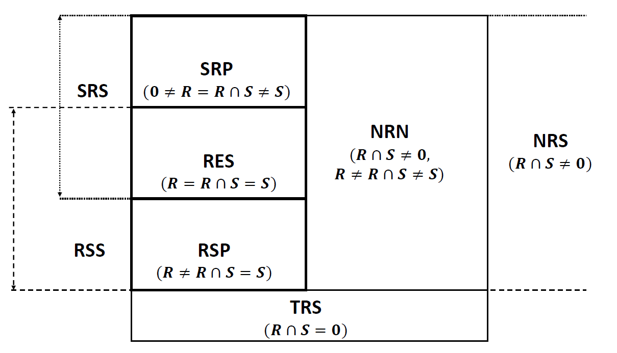
The following Theorem provides the relationship between and the network classes:
Theorem 2.
(Arceo et al. [3]) Let be the map of complexes of a network with subnetwork of -complexes.
- i)
is Furthermore, is
- ii)
is Furthermore, is either or
- iii)
is is a direct sum of ans Furthermore, is and, if has no inflow reaction,
- iv)
is Furthermore, is
Arceo et al. [3] showed that had the distinctive property of being a union of linkage classes. We now show that this derives from the fact that is part of a -decomposition which we call the -decomposition. We have the following Lemma:
Lemma 1.
For any reaction , either both complexes and are in or none of them.
Proof.
If is in , then is also in . Similarly, in implies is in ∎
Definition 20.
A reaction is an -reaction if both complexes and are in . denotes the set of -reactions, the subnetwork-complement decomposition it induces is called the -decomposition.
The -decomposition is clearly a -decomposition, and hence its subnetworks and are unions of linkage classes. Theorem 2 provides a good example showing that in NRN network, is non-empty.
We also obtain a new characterization of the ILC property:
Corollary 4.
A network has independent linkage classes if and only if every -decomposition is independent.
Proof.
If a network has independent linkage classes then the stoichiometric subspace is the direct sum of the stoichiometric subspaces of the linkage classes. Grouping the summands according to the unions of the linkage classes for the subnetworks of a -decomposition provides as the direct sum of the subnetworks. Hence, every -decomposition of a network is also independent. For the converse, since every -decomposition of a network is independent and the linkage class decomposition is also a -decomposition, it follows that the linkage classes are independent. ∎
If a network has dependent linkage class, it may fail to have an independent -decomposition, as the following example shows:
Example 3.
Consider the CRN with reactions and , it has . The only non-trivial decomposition is the linkage class decomposition, where the deficiency of the two linkage classes is 0. Clearly, the linkage class decomposition is dependent. In particular, it has no independent -decomposition.
3.4 Incidence independent decompositions and complex balanced equilibria
Feinberg established the following basic relation between an independent decomposition and the set of positive equilibria of a kinetics on the network:
Theorem 3.
(Feinberg Decomposition Theorem [9]) Let be a partition of a CRN and let If is a network decomposition of and then
If the network decomposition is independent, then equality holds.
Our main result in this section is the analogue of Feinberg’s 1987 result for incidence independent decompositions and complex balanced equilibria:
Theorem 4.
Let be a CRN and be the subnetworks of a decomposition. Let be any kinetics and and be as defined above. Then:
- i)
If the decomposition is incidence independent, then - ii)
- iii)
then for each .
Proof.
are not assumed weakly reversible, so may be empty. Let be the reaction subset defining and is given by where is the projection from to Furthermore set Then Clearly, in i) if the LHS is empty, there is nothing to prove. If , then for each , and hence their sum , or .
To show ii), again if the LHS is empty, then we are done. If , then Since the decomposition is incidence independent, it follows that for each , or Note that in this case, and are necessarily weakly reversible. Equality then follows from i). iii) follows directly from ii). ∎
The converse statement of Theorem 4 (iii) holds for a subset of incidence independent decompositions with any kinetics. This is a significant contrast to the case of independent decompositions where the converse statement is known only for a few restricted kinetics such as MAK and PL-TIK, which are power law kinetics with zero kinetic reactant deficiency [24]. To show this part of our second main result, we need the following proposition:
Proposition 10.
Theorem 5.
Let be a weakly reversible -decomposition of a chemical kinetic system Then, if for each subnetwork,
Proof.
We first consider the case when the -decomposition is the linkage class decomposition. It is well known that the incidence map has a block matrix decomposition, after the complex rows are arranged as and the reaction columns as respectively:
Furthermore, a complex balanced equilibrium of and is the image of contained in and respectively. Since the -decomposition is incidence independent, is the direct sum of the images of the incidence maps of the subnetworks. In view of the block matrix description of , we also obtain that is the direct sum of the images of the transposed maps on the subnetworks. Hence, Proposition 10 is applicable and we have:
| (3.2) |
In Theorem 1, it is shown that any -decomposition is generated by a coarsening of the partition of the reaction set into the reaction sets of linkage classes. This implies that the incidence map of the subnetworks are groupings of the terms in Equation 3.2 and hence the intersection is taken over the same sets of equilibria, which proves the claim. ∎
Remark 1.
The two previous Theorems were derived for the special case of the linkage class decomposition and poly-PL kinetics in [25].
The following tables emphasize the analogous characteristics of independent and incidence independent decompositions:
| Independent decomposition: characteristic | Reference/Comment |
|---|---|
| Definition: is direct sum of subnetwork | Feinberg 1987 [9] |
| Deficiency relationship: | Fortun et al. 2018 [12] |
| Equilibria sets for any kinetics: | Feinberg 1987 [9] |
| Coarsening invariance: any coarsening of an | this paper |
| independent decomposition is also independent |
| Incidence Independent decomposition: characteristic | Reference/Comment |
|---|---|
| Definition: is direct sum of subnetwork | this paper |
| Deficiency relationship: | this paper /linkage class |
| case: Feinberg 1987 [9] | |
| CB Equilibria sets for weakly reversible decomposition and | this paper /linkage class |
| any kinetics: | and PY-RDK case: |
| Talabis et al. 2018 [25] | |
| Coarsening invariance: any coarsening of an incidence | this paper |
| independent decomposition is also incident independent |
3.5 -decompositions
In their S-system model of Mtb gene regulation, Magombedze and Mulder [17] introduced three subsystems, which in the CRN representation generated a decomposition into three subnetworks, whose sets of non-zero complexes were pairwise disjoint. This led us to define the set of -decompositions of chemical reaction networks and study their properties.
Definition 21.
A decomposition with is a -decomposition if for where and are the non-zero complexes in and , respectively.
Clearly, the set of -decompositions is contained in this set.
Remark 2.
Gross et al. [14] call the union of two networks “complex-disjoint” if the intersection of their sets of complexes is contained in If the covering defined by the union is a decomposition, then this construct is identical with a -decomposition. However, we find their terminology somewhat confusing since the zero complex is a bona fide complex. In our view, the “complex-disjoint” decompositions are the -decompositions.
The following Theorem describes the general structure of -decompositions.
Theorem 6.
(Structure Theorem for -decomposition) Let be a -decomposition and and be the linkage classes of and containing the zero complex (note , is empty if does not contain the zero complex). Then
- i)
the form a -decomposition of
- ii)
the (non-empty) form a -decomposition of
Proof.
To prove (i), we need to show that each non-zero complex of is contained in only one subnetwork . If there is only one subnetwork containing the zero complex then we are done. If there are at least two subnetworks containing the zero complex then has at least two non-zero complexes connected to the zero complex. Otherwise, if there would only be one complex then is not a -decomposition of , a contradiction. Now, if one of these non-zero complexes belongs to different subnetworks, this would contradict that partitions the non-zero complexes. Hence, all the non-zero complexes of is contained in only one and for .
To prove (ii), it suffices to show that the intersection of the set of complexes in is empty. The set of complexes in are all non-zero and . From (i), we have for . Thus, where is empty if does not contain the zero complex. Since is a -decomposition of , the intersection of the set of complexes in is empty. ∎
We will now use the previous result to prove the incidence independence of -decompositions. The number of subnetworks containing the zero complex turns out to be a useful tool for this. If , then the network does not contain the zero complex, hence the set of -decompositions is simply the set of -decompositions. For positive values, it can be used to formulate a convenient criterion for incidence independence:
Corollary 5.
Any -decomposition is incidence independent.
Proof.
We recall from Equation (3.1) that
where and are number of complexes and linkage classes in the subnetwork .
Suppose . If subnetworks contain the zero complex then the number of complexes , where is the number of non-zero complexes. For any of the subnetworks, for the corresponding numbers, we also have , for all others, Thus, Equation (3.1) becomes
Since , we obtain ∎
According to the Structure Theorem, the linkage classes of consist of and such which contain only non-zero complexes, Each of these remaining linkage classes must however be contained in exactly one subnetwork, and hence a linkage class of that subnetwork. Conversely, each linkage class in a subnetwork with only non-zero complexes is a linkage class of the whole network. Therefore where the first sum is over all subnetworks not containing and the second over all subnetworks containing . Therefore which is the formulated criterion for incidence independence above.
4 Species coverable CRNs and S-system realizations
In this Section, we introduce a new realization of an S-system in order to enable a CRNT approach in the context of recent developments in BST on phenotype-oriented modeling based on design spaces. This realization will be defined in the framework of total realizations of BST systems in Section 4.1.2. In order to study the new and old S-system realizations in a semantically consistent manner, we introduce the class of species coverable CRNs and its subset of species decomposable CRNs. Our main result in this Section, Theorem 7, corrects and extends a deficiency formula by Arceo et al. [1] and a result by Hernandez et al. [15] to species decomposable CRNs.
4.1 S-systems and their realizations
4.1.1 Current realization of an S-system
To any given S-system, Arceo et al. associated the biochemical map (see Figure 2) and obtained CRNs which they called stoichiometric and total representations [1]. To obtain a realization, i.e. a dynamically equivalent kinetic system, they constructed in [2] the embedded network of the total representation given by the subsets of dependent species and the full reaction set. This realization, called the embedded representation, has the advantage of using the minimum number of species needed and corresponded to the BST practice of “lumping” the independent variables with the rate constants for each power law term.

Let and be the sets of the variables regulating the input and output arrow for (as in Figure 2) and be the sums of the elements in and respectively. In this realization, the reaction subsets have the following property:
Proposition 11.
The reaction sets form an independent decomposition of the embedded representation.
Proof.
i) We have to show that if , then the intersection of the reaction sets is empty. Suppose that the sets do not form a partition of the reaction set . Then there exists two sets and , where , that has a common reaction. We consider the following cases: a) two inflow reactions coincide and b) an inflow reaction coincides with an outflow reaction. The remaining cases involve converse reactions and hence follow similarly.
We let and . We denote the subvectors of and as and , respectively. We set and . In connection to the elements of , the two input reactions in and coincide thus and . This implies that and or . Since , and , a contradiction.
As for the elements of , we assume that an inflow reaction in coincides with an . Then and . Thus, we have or . This implies that and . Similarly, implies that and . Since , and , a contradiction.
ii) Note that the stoichiometric subspace of each of the subnetworks of the species decomposition is . Thus, the rank of each is 1. Since there are subnetworks and the rank of an -system is m, and this implies independence. ∎
4.1.2 Total realization of a BST system
We now introduce an additional realization for any BST system, in particular, any GMA system given by a biochemical map:
Definition 22.
The total realization of a BST system is the total representation with an additional outflow reaction for each independent variable together with the power law kinetics specified by the kinetic order matrix.
The additional outflow reaction for each independent variable enables the corresponding ODE to be solvable in all cases, hence, resulting in a realization of the GMA system. Clearly, the total realization has the same sets of species and complexes as the total representation, but has additional reactions number of independent species).
Example 4.
Note that the embedded networks formed by the subset of dependent species and all reactions of total representations and the total realizations are identical. For consistency in terminology, we will henceforth denote the embedded representations as “embedded realizations” of the BST systems.
4.2 Subnetwork realization of an S-system
In BST´s design space theory [23], a phenotype-oriented analysis of the behavior of a biochemical system described by a GMA model is conducted by constructing S-subsystems and identifying parameter regions where the S-subsystem is dominant, i.e. its values determine the behavior. The initial step in design space theory selects for each dependent variable, a positive (activating) and a negative (degrading) term from its ODE. In the GMA system´s biochemical map, this amounts to selecting an input arrow and an output arrow for each dependent variable. In the CRN of the total realization, we obtain a subnetwork defined as follows:
Definition 23.
The subnetwork realization of an S-subsystem of a GMA system is the total realization of the union of the subnetworks generated by the reaction pairs for each dependent species , where , being the sums of the corresponding regulatory species of the input and output arrows. The sets of reaction pairs form the species covering of the subnetwork realization.
As the simple example, shows, this species covering is not necessarily a decomposition, since several inflow reactions coincide with previous outflow reactions: in fact, there are only reactions instead of
Remark 3.
The terminology “independent realization” of an S-system highlights the fact it is represented independently of any containing network/system. Fortuitously, the subsets of reaction pairs also form an independent decomposition of the independent realization.
4.3 Species coverable and species decomposable CRNs
Despite its contrasting semantic interpretation to the subnetwork realization, we readily observe that formally the independent realization is a special case of the subnetwork realization: if we set we obtain the independent realization. In order to have a consistent semantic framework, we abstract a level further and introduce a class of CRNs containing the networks of both realizations. We then use this class to formulate and derive common properties.
Definition 24.
- i)
A CRN with species set is species coverable if for each , there are species and subsets of with be the sums of their respective elements such that is the union of with The ’s form the species covering of the network.
- ii)
A species is called independent if and (hence by convention, Otherwise, it is a dependent species. A species is reversible if (hence all independent species are reversible).
- iii)
A species coverable CRN is species decomposable if the species covering is an independent decomposition.
Example 5.
- 1.
The CRN of the subnetwork realization of an S-system is species coverable
- 2.
The CRN of the independent realization of an S-system is species decomposable.
We have the following main result for species decomposable CRNs:
Theorem 7.
Let be a species decomposable CRN. Then
- i)
where is the number of reversible species. If the species decomposition is bi-independent, then
- ii)
the fundamental decomposition of is the species decomposition.
Proof.
- i)
Since the species decomposition is independent, . Since , this implies that and . For a reversible species , we have . For an irreversible species, we have either or . Hence Hence, since the decomposition is independent. If it is also incidence independent, then holds.
- ii)
We denote the inflow reaction in with , and the corresponding basis vector with and , respectively. We set , and as remarked above, since the species decomposition is independent, the network is open (i.e. and for each . Hence for any orientation, the cardinality , and . For each irreversible species , we can write
We claim that the vectors lie in
They are linearly independent and hence form a basis. On the other hand, the vectors with and and the reaction from a reversible pair included in the orientation, form a basis for From the -decomposition definition, the reactions and are equivalent, If so that if is nonzero, then the -th inflow reaction is not equivalent. Similarly, the -th outflow reaction is not equivalent. Hence, the -equivalence classes are precisely the
∎
Remark 4.
Since in Proposition 3.19 of [15], for all , there is a typo in the proof: instead of “” it should read “”.
Finally, we note the following new formulation of Theorem 3 in [8].
Theorem 8.
Any species coverable CRN with two or more dependent species is discordant.
Remark 5.
For positive equilibria, we have the following hierarchy of subsets and CRN classes in which they may exist: detailed balanced (DB) equilibria (reversible CRNs) complex balanced (CB) equilibria (weakly reversible CRNs) positive equilibria (any CRN). This hierarchy corresponds to balance of the level of reactions (DB), to balance on the level of complexes (CB) and balance on the level of species.
With the introduction of species decomposable CRNs, we obtain the following (restricted) conceptual hierarchy:
- •
(level of reactions), for any CRN, any decomposition determines (is in fact equal to) a partition of the set of reaction
- •
(level of complexes), for any CRN, any -decomposition, in addition, determines a partition of the set of complexes
- •
(level of species) for any species decomposable CRN, the fundamental decomposition (= species decomposition) determines a partition of the set of species (into singletons)
The restriction is of course that the species level is valid only for a small class of CRNs.
5 Conclusions and outlook
This paper presents novel decomposition classes of chemical reaction networks (CRNs) derived from S-system kinetics:
We introduced the concept of coverings, a minor generalization of a decomposition, and relate it to the unions of CRNs. A covering is called a decomposition of if the sets form a partition of . Given the network covering properties, we introduced the basic property of incidence independent decompositions of a CRN, which complements the independence property defined by M. Feinberg in 1987 [9]. We have shown in Proposition 7 that for an incidence independent decomposition , .
In this paper, we have presented the following new results:
- •
The theory of - and - decompositions which partition the set of complexes and the set of nonzero complexes respectively, including their structure theorems in terms of linkage classes (shown in Theorem 1 and Theorem 6, respectively). We have shown that and - decompositions are both incident independent (shown in Corollary 3 and Corollary 5, respectively).
- •
- •
We have introduced a new realization for an S-system that is analyzed using a newly defined class of species coverable CRNs (see Definition 24). This led to the extension of the deficiency formula and characterization of fundamental decompositions to species decomposable reaction theorem (Theorem 7).
Acknowledgments. HFF acknowledges the support of the Commission on Higher Education (CHED), Philippines for the CHED-SEGS Scholarship Grant. ARL held research fellowship from De La Salle University and would like to acknowledge the support of De La Salle University’s Research Coordination Office.
References
- [1] C.P.P. Arceo, E.C. Jose, A. Marin-Sanguino, E.R. Mendoza, Chemical reaction network approaches to biochemical systems theory, Math. Biosci. 269 (2015) 135–152.
- [2] C.P.P. Arceo, E.C. Jose, A.R. Lao, E.R. Mendoza, Reaction networks and kinetics of biochemical systems, Math. Biosci. 283 (2017) 13–29.
- [3] C.P.P. Arceo, E.C. Jose, A.R. Lao, E.R. Mendoza, Reactant subspaces and kinetics of chemical reaction networks, J. Math. Chem. 56(2) (2018) 395–422.
- [4] B. Boros, On the positive steady states of Deficiency-One Mass Action Systems, Eotvos Lorand University (2013) Ph.D. thesis
- [5] G. Craciun, F. Nazarov, C. Pantea, Persistence and permanence of mass action and power law dynamical systems, SIAM J. Appl. Math. 72 (2013) 305–329.
- [6] A.R. Chowdhury, C. Madhu, Network decomposition based large-scale reverse engineering of gene regulatory network, Neurocomput. 160 (2015) 213–227.
- [7] P. Donnell, M. Banaji, A. Marginean, C. Pantea, Control: an open source framework for the analysis of chemical reaction networks, Bioinformatics. 30(11) (2014) 1633–1634.
- [8] H.F. Farinas, E.R. Mendoza, A.R. Lao, Structural properties of an S-system model of Mycobacterium tuberculosis gene regulation. (2020, submitted)
- [9] M. Feinberg, Chemical reaction network structure and the stability of complex isothermal reactors: I.The deficiency zero and deficiency one theorems, Chem. Eng. Sci. 42 (1987) 2229–2268.
- [10] M. Feinberg, F.J.M. Horn, Chemical mechanism structure and the coincidence of the stoichiometric and kinetic subspaces, Arch. Rational Mech. Anal. 66 (1977) 83–97.
- [11] E. Feliu, C. Wiuf, Preclusion of switch behaviour in networks with mass action kinetics, Appl. Math. Comput. 219 (2012) 1449–1467.
- [12] N. Fortun, A.R. Lao, L.F. Razon, E.R. Mendoza, A deciency zero theorem for a class of power law kinetic systems with reactant determined interactions, J. Math. Chem. 56(10) (2018) 2929–2962
- [13] N.T. Fortun, E.R. Mendoza, L.F. Razon, A.R. Lao, A Deficiency Zero Theorem for a class of power law kinetic systems with non-reactant determined interactions, MATCH Commun. Math. Comput. Chem. 81 (2019) 621–638.
- [14] E. Gross, H. Harrington, N. Meschkat, A.J. Shiu, Joining and decomposing reaction networks. (2019, submitted)
- [15] B.S. Hernandez, E.R. Mendoza, A.A. de los Reyes, Fundamental Decompositions and Multistationarity of Power-Law Kinetic Systems. MATCH Commun. Math. Comput. Chem. 83 (2020)(2) 403–434.
- [16] F. Horn, R. Jackson, General mass action kinetics, Arch. Ration. Mech. Anal. 47 (1972) 81–-116.
- [17] G. Magombedze, N. Mulder, Understanding TB latency using computational and dynamic modelling procedures, Infect. Genet. Evol. 13 (2013) 267–283.
- [18] O.B. Mahfuz, D. Showkat, Inference of Gene Regulatory Network with S-system and Artificial Bee Colony Algorithm, 2018 Joint 7th International Conference on Informatics, Electronics & Vision (ICIEV) and 2018 2nd International Conference on Imaging, Vision & Pattern Recognition (icIVPR), (2018) 117-122.
- [19] S. Müller, G. Regensburger, Generalized mass action systems: Complex balancing equilibria and sign vectors of the stoichiometric and kinetic-order subspaces, SIAM J. Appl. Math. 72 (2012) 1926–-1947.
- [20] S. Müller, G. Regensburger, Generalized Mass-Action Systems and Positive Solutions of Polynomial Equations with Real and Symbolic Exponents (Invited Talk). In: Gerdt V.P., Koepf W., Seiler W.M., Vorozhtsov E.V. (eds) Computer Algebra in Scientific Computing. CASC 2014. Lecture Notes in Computer Science 8660 (2014) 302–323.
- [21] M.A. Savageau, Biochemical systems analysis. I. Some mathematical properties of the rate law for the component enzymatic reactions, J. Theor. Bio. 25 (1969) 365–369.
- [22] M.A. Savageau, Biochemical systems analysis. II. The steady-state solutions for an n-pool system using a power law approximation, J. Theor. Bio. 25 (1969) 370–379.
- [23] M.A. Savageau, P.M. Coelho, R.A. Fasani, D.A. Tolla, A. Salvadoe. Phenotypes and tolerances in the design space of biochemical systems. Proc Natl Acad Sci USA (2009) 106 (16): 6435–6440.
- [24] D.A.S. Talabis, E.R. Mendoza, E.C. Jose, Complex balanced equilibria of weakly reversible power law kinetic systems, MATCH Commun. Math. Comput. Chem. 82(2019) 601–624
- [25] D. A. S. Talabis, D. M. Magpantay, E. R. Mendoza, E. G. Nocon, E. C. Jose. Complex Balanced Equilibria of Weakly Reversible Poly-PL Kinetic Systems and Evolutionary Games, MATCH Commun. Math. Comput. Chem. 83 (2020)(2) 375-402
- [26] E.O. Voit, Computational Analysis of Biochemical Systems, Cambridge Univ. Press, Cambridge, 2000.
- [27] E.O. Voit, Biochemical Systems Theory: A Review, ISRN Biomath. 2013 (2013) 1–-53. doi:10.1155/2013/897658.