Deep modeling of quasar variabilityJournal: ApJ
Abstract
Quasars have long been known as intrinsically variable sources, but the physical mechanism underlying the temporal optical/UV variability is still not well understood. We propose a novel nonparametric method for modeling and forecasting the optical variability of quasars utilizing an autoencoder neural network to gain insight into the underlying processes. The autoencoder is trained with 15,000 decade-long quasar light curves obtained by the Catalina Real-time Transient Survey selected with negligible flux contamination from the host galaxy. The autoencoder’s performance in forecasting the temporal flux variation of quasars is superior to that of the damped random walk process. We find a temporal asymmetry in the optical variability and a novel relation – the amplitude of the variability asymmetry decreases as luminosity and/or black hole mass increases – is suggested with the help of autoencoded features. The characteristics of the variability asymmetry are in agreement with those from the self-organized disk instability model, which predicts that the magnitude of the variability asymmetry decreases as the ratio of the diffusion mass to inflow mass in the accretion disk increases.
Keywords:
methods: statistical; quasars: general; accretion disksI Introduction
Quasars are a key population for investigating and understanding the physics of accretion of matter under extreme physical conditions. Several hundred thousand quasars have been spectroscopically confirmed so far and many attempts have been made to determine the characteristics of their temporal flux variability. However, the physical mechanisms underlying the variability remain poorly understood, in part due to the difficulty in parameterizing its aperiodicity.
In the optical/UV, it is only the variability amplitude and its correlation with timescale that have so far been suggested to be related to intrinsic physical parameters. For example, the amplitude of quasar optical variability increases with decreasing luminosity, restframe wavelength, and Eddington ratio (e.g., Wills et al. 1993; Giveon et al. 1999; Vanden Berk et al. 2004), and the structure function tends to possess a steeper slope for quasars with a larger black hole mass (Caplar et al. 2017). The correlation with black hole mass is still unclear, however, with different studies advocating either positive or negative relationships (e.g., Wold et al. 2007; Kelly et al. 2009; Zuo et al. 2012), depending on the degree to which observational biases have been eliminated. Physical mechanisms underlying the optical/UV variability have been proposed: the superposition of supernovae (Aretxaga et al. 1997; Kawaguchi et al. 1998), microlensing (Hawkins 1993; Hawkins 2010), thermal fluctuations from magnetic field turbulence (King et al. 2004; Kelly et al. 2009; Kelly et al. 2011), and instabilities in the accretion disk (Takeuchi et al. 1995; Kawaguchi et al. 1998).
Recently a large attempt has been made to reveal the latent physical process underlying extremely large flux variations ( 1 mag) in quasars. Tidal disruption events (TDEs), large amplitude microlensing, a large change of obscuration or accretion rate, and supernovae have been proposed for such extreme temporal variabilities (e.g., Meusinger et al. 2010; Drake et al. 2011; Bruce et al. 2016; Lawrence et al. 2016; Ruan et al. 2016; Graham et al. 2017a; Stern et al. 2018; Ross et al. 2018; Assef et al. 2018), but it remains unclear whether or how they relate to the more general optical variability seen in quasars.
To describe quasar optical variability, Kelly et al. 2009 proposed a continuous time first-order autoregressive model, also known as the Ornstein-Uhlenbeck or damped random walk (DRW) process, which is a particular type of Gaussian process characterized by two parameters: , the relaxation time, and , the variability on timescales much shorter than . Several authors have shown that the DRW process provides a better statistical model for most quasar variability when compared to a range of alternative stochastic/deterministic models (e.g., Andrae et al. 2013). However, Kozłowski 2017, pointed out that the best-fit DRW processes are biased in due to an insufficient temporal baseline in existing surveys for probing the white noise portion of the power spectral density (PSD). This paper shows that a temporal baseline at least ten times longer than is necessary to properly constrain . Any reported correlations between these model parameters and physical parameters, such as black hole mass or Eddington ratio, are therefore potentially analysis artifacts. Additionally, deviations from a DRW process in quasar variability have begun to be recognized. Kepler light curves with 30 min sampling revealed a steeper power-law index of about at very high frequency (less than a few months; e.g., Mushotzky et al. 2011; Kasliwal et al. 2015), which is a significant deviation from the DRW process. On very long timescales (at lower frequencies than the typical timescale of a quasar light curve), Guo et al. 2017 found that the observed residual scatter in is too large for uncertainties in the DRW process parameter derived from 1,678 light curves of low redshift quasars with low black hole mass. They also suggested that the scatter can be explained if the low frequency PSD slope is about . Mushotzky et al. 2011 concluded that individual quasars exhibit intrinsically different PSD slopes, indicating that the DRW process is too simplistic to describe optical quasar variability (e.g., Graham et al. 2014; Kasliwal et al. 2015; Caplar et al. 2017). The situation would likely be even worse for more complex stochastic models. More phenomenological parameters would be even more difficult to connect with underlying physical processes.
In this work, we present an initial application of the autoencoder, which is a type of unsupervised (deep) machine learning algorithm, to quasar temporal flux behavior by assuming that quasar temporal variability can be represented in a low dimensional space. The training and the validation of the model is performed with quasar light curves obtained by the Catalina Real-time Transient Survey (CRTS;11 1 http://crts.caltech.edu Drake et al. 2009; Mahabal et al. 2011), which is the largest open (publicly accessible) time domain survey currently available. The representative expressions or characterizing features of temporal variability are acquired by the autoencoder itself in an unsupervised way, and thus modeling and forecasting is performed without any prior assumptions. We also propose a methodology for associating the representative expressions (autoencoded features; AE features) with physical parameters utilizing a simple multilayer perceptron (MLP) and then show its validity.
This paper is structured as follows: in section 2, we describe the method and data selection and in section 3, the results of applying the autoencoder to extract features and to forecast quasar variability. Section 4 discusses the features and their relation to physical parameters and models. Section 5 presents our conclusions. Alongside this paper, the scripts used for the analysis shown in this work are available online22 2 https://github.com/yutarotachibana/CatalinaQSO_AutoEncoder.
II Method
In this section, we discuss CRTS, the photometric calibration method employed by the pipeline of the survey project, the data selection criteria we employ in this work, and the basic structure of the autoencoder we use to model and forecast quasar variability.
II.1 Catalina Real-time Transient Survey
The CRTS archive33 3 http://catalinadata.org contains the Catalina Sky Survey data streams from three telescopes – the 0.7 m Catalina Sky Survey (CSS) Schmidt and 1.5 m Mount Lemmon Survey (MLS) telescopes in Arizona, and the 0.5 m Siding Springs Survey (SSS) Schmidt in Australia. These surveys, operated by the Lunar and Planetary Laboratory at the University of Arizona, were designed to search for near-Earth objects, but have proven extremely valuable for astrophysics topics ranging from Galactic transients (Drake et al. 2014) to distant quasars (Graham et al. 2014; Graham et al. 2015; Graham et al. 2017a). CRTS covers up to 2500 deg2 per night, with 4 exposures per visit, separated by 10 min. The survey observes over 21 nights per lunation. The data are broadly calibrated to Johnson (see Drake et al. 2013 for details) and the current CRTS data set contains time series for approximately 400 million sources to above Dec from 2003 to 2016 May (observed with CSS and MLS) and 100 million sources to in the southern sky (Dec) from 2005 to 2013 (from SSS).
There are few data sets with sufficient sky coverage, temporal coverage, and sampling to enable us to investigate quasar optical variability systematically. The largest data sets which can be used for research on the long term optical variability of quasars currently are SDSS with POSS, Pan-STARRS1 (e.g., MacLeod et al. 2012; Morganson et al. 2014), and CRTS. Among these, CRTS provides the best dataset for investigating the temporal flux variation on timescales from weeks to decades due to its large number of objects and observation cadence.
The error model used for CRTS is incorrect: errors at the brighter magnitudes are overestimated and those at fainter magnitudes () are underestimated (Palaversa et al. 2013; Drake et al. 2014). In this analysis, we employ the improved error model derived in Graham et al. 2017b; the actual CRTS error model will be fixed in a future release. We apply the same preprocessing steps described in Graham et al. 2015 to all light curves, which remove outlier photometric points and combine all exposures for a given night to give a single weighted value for that night. We also remove sources associated with nearby bright stars or identifiable as blends from a combined multimodality in their magnitude and observation position, i.e., the spatial distribution of all points in a light curve is best described by Gaussians.
II.2 Data Selection
We have crossmatched 555,692 sources classed as “QSO” in SDSS DR15 (Aguado et al. 2019) against the CRTS data set with a 3” matching radius. We selected objects within the magnitude range to minimize systematic effects from error estimation and saturation and excluded known blazars. 40,736 spectroscopically confirmed quasars lie within these ranges in CRTS.
To check the characteristics of the quasars, we calculated the variance of the light curves and the optical luminosities, where the intrinsic variance is referred to as the variance in this paper, and is described by:
| (1) |
where is the number of data points, and are the observed magnitude and its uncertainty, respectively, and is the weighted average of the magnitudes. The optical luminosity () can be approximately calculated by:
| (2) |
where is the luminosity distance calculated with , , and (Jarosik et al. 2011), Å-1 is the zero point flux density,44 4 http://svo2.cab.inta-csic.es/svo/theory/fps3/index.php?id=Misc/CRTS.C Å is the effective wavelength of the CRTS filter system (see Fig. 1), and is the Galactic absorption at the effective wavelength along the line-of-sight. The CRTS Galactic absorption is estimated based on the total extinction in the -band provided by IRSA,55 5 https://irsa.ipac.caltech.edu/applications/DUST/ obtained by using the Python package astroquery.66 6 https://astroquery.readthedocs.io/en/latest/irsa/irsa_dust.html The extinction in the -band can be translated to that at through an empirical relation between Å and given by O’Donnell 1994, where we adopt . The extinction package77 7 https://extinction.readthedocs.io/en/latest/#extinction is used for converting to . Fig. 2 shows the distributions of redshift, mean magnitude, optical luminosity, and variance for the quasar sample. The histograms colored by green and red overplotted on the gray histograms indicate the distribution of sources identified as an extended source or as a point source in their respective PS1 image (Tachibana & Miller 2018).88 8 Strictly speaking, a PS1 counterpart within 1 arcsec from a CRTS quasar. One can see that there are two obvious classes in the data set: (1) resolved, nearby, intrinsically fainter, and lower variable sources, and (2) unresolved, far away, intrinsically brighter, and higher variable sources.
The two groups are clearly distinguishable in the – plane, as shown in Fig. 3. This behavior can be interpreted as the combination of flux coming from the stable host galaxy and the partially-visible variable accretion disk. Significant flux contamination at the faint end is unavoidable as CRTS measurements are produced by aperture photometry (see Section II.1) and so a part of the resolved host galaxy must be inside the aperture used. For sources brighter than , the variance and luminosity are anticorrelated, which is consistent with previous research mentioned in Section I. We are therefore able to identify sources showing variability purely originating from the disk with .
15,438 quasars were selected, which should contain minimal flux contamination from the host galaxy.99 9 In addition to the luminosity threshold, sources with , d, and , are selected, where and is the observation length and the number of observations, respectively. This selection is crucial to investigate quasar variability, namely disk variability, because the contamination significantly suppresses the variation amplitude at its faint state and we cannot subtract the contamination from the total brightness as we do not know the true flux level of the host galaxy.
II.3 Simulated Light Curves
Simulated light curves are commonly used to assess systematic biases because observational biases such as observation gaps (i.e., the window function of the observation), which can generate systematic and puzzling results (e.g., Suberlak et al. 2017), should show in analysis results for both the real and the simulated data. Since the expected behavior for optical quasar variability is that it approximately follows a DRW process (see Section I), we generate simulated light curves using the actual observation times, but replacing the observed magnitudes with expected values under a DRW process.
Formally, the temporal behavior of a DRW process is given by:
| (3) |
where is a white noise process with zero mean and variance equal to 1 and . The corresponding likelihood function involves an exponential covariance matrix:
| (4) |
The model parameters for the simulated light curves, , and , are the same as those derived from the DRW process fit to the associated quasar light curve. In addition, we added a Gaussian deviate derived from the empirical function:
| (5) |
fit to the quasar dataset, and the modeled error is treated as the measurement uncertainty on the simulated light curves. Note that both fitting and simulation is in the quasar restframe.
Examples of observed and simulated quasar light curves are displayed in Fig. 4. The interpretation of analysis results is performed by comparison between the results for the two data sets.
II.4 Autoencoder Neural Network

An autoencoder is a type of unsupervised neural network which is trained to reconstruct the original input while compressing the data in the process so as to discover a more efficient and reduced representation in an internal (hidden) layer. The main purpose of this architecture is dimension reduction and as the number of nodes in the hidden layer is smaller than in the input and output layers, fundamental information should be condensed at the layer with the smallest number of nodes. This architecture facilitates classification and also optimum modeling of the input data.
For sequence-to-sequence data, the autoencoder can be implemented using a recurrent neural network (RNN; see Lipton et al. 2015, for a review) architecture. Traditional neural networks assume that all inputs (and outputs) are independent of each other but RNNs perform the same task for every element of a sequence with the output at a particular timestep forming part of the input to the next timestep. This means that information is retained about what has been calculated so far and this can affect the current calculation and prediction. RNNs have been used in astronomy for time series classification (Charnock & Moss 2017; Naul et al. 2018; Becker et al. 2020). The RNN autoencoder network is trained with time series as input to reproduce the same time series as the output. The coded representation in the hidden layer is thus a time-dependent compression and can be interpreted as features of the input time series. With these features, Naul et al. 2018 demonstrated that the accuracy of supervised variable star classification is superior to or at least consistent with that of a classifier with expert-chosen hand-selected features.
The autoencoder neural network that we constructed for modeling and forecasting quasar light curves is displayed in Fig. 5. This network uses two LSTM1010 10 Long short time memory (LSTM) is a type of RNN; for detailed information about LSTMs, see Jain & Medsker 1999. layers of size 32 for encoding (reducing the input) and two for decoding (reconstructing the input), with an autoencoded feature size of 16 (AE features hereafter). We input the measurement values, the differences between sampling times (to deal with the irregular time sampling of the data), and the measurement errors. Since we are also interested in forecasting, we have excluded the last 500 days of data for each source. The AE features are constructed by passing the output of the last recurrent encoding layer into a single fully-connected layer with a linear activation function and the desired output size. The decoder repeats the AE features times, where is the length of the next layer, 32 in this architecture, and then appends the values to the corresponding elements of the resulting vector sequence. The decoder network is constructed from another series of LSTM layers, with a final linear layer to generate the original light curve, i.e., the output is 500 days longer than the input data. The model, therefore, performs modeling and forecasting simultaneously. The loss (weighted mean squared error) is defined by:
| (6) |
where is the number of light curves, and , , and are the th measurement, reconstruction value, and measurement error of the th light curve, respectively; this reduces the penalty for reconstruction errors when the measurement error is large. We also apply a 25% dropout between LSTM layers to generalize the ability to model and forecast quasar light curves. We note that the architectural hyperparameters of the network, i.e., the number of layers, number of nodes per layer, number of nodes in the hidden layer, etc., are arbitrarily chosen to provide a network similar to the one employed by Naul et al. 2018. Bayesian optimization of these quantities is possible but can be computationally expensive and by experimentation we found that the results of the network were robust to changes by factors of two in the values used here.
III Result
III.1 Training the Autoencoder
To train and validate the autoencoder shown in Fig. 5, we divided the quasar dataset into a training dataset (80%; 12,350 sources) and a validation dataset (20%; 3,088 sources). The input () and the target magnitudes () are normalized by the average and the standard deviation of the input magnitude;
| (7) | ||||
| (8) |
Also for and , the normalizations and are applied. We note that the inputs do not have any information on the forecasting part (the last 500 days) as we used only and for the normalization of both the input and the output.
Fig. 6 shows the loss (see eqn. 6) for the training dataset and the validation data set. We used Adam optimization (Kingma & Ba 2014) with standard parameter values , , a learning rate of and a batch size of 256. All models are implemented with the Keras package.1111 11 https://keras.io/ The top panel in Fig. 6 shows that both the validation loss and the training loss decrease as a function of the training epoch. While the training loss and the validation loss values cross at the training epoch of 8000, no obvious signal of overfitting is seen. The final loss for the validation dataset is 4.25, which might seem somewhat large for a reduced chi-square , but is acceptable as the loss is calculated for both the modeling part and the forecasting part of the output.
The middle panel in Fig. 6 shows the forecasting accuracy evaluated from the difference of the reduced chi-square (; see Eq.(6)) of the autoencoder model (AE model; ) and the DRW process model (DRW model; , see Eq.(III.2)) for time ranges and , where is the time difference from the beginning of the forecasting part of the output. and is thus the first half and the latter half of the forecasting part, respectively. Since the accuracy of the AE model is defined by , a smaller value indicates a higher accuracy. As shown in Fig. 6, the forecasting accuracy increases as the training proceeds.
In addition, we have confirmed that the AE features actually acquire information on physical parameters as training proceeds. The bottom panel in Fig. 6 shows the correlation coefficient and the partial correlation coefficient between the AE features and optical luminosity, where these values are calculated on the validation data set. For the partial correlation coefficient, the variance of the light curve, which is known to be correlated with optical luminosity, is considered to be a latent variable, and its effect is removed from the correlation coefficient (see Section III.4 for the method to calculate the correlation coefficient between the AE features and a physical parameter). The partial correlation coefficient can be calculated by:
| (9) |
where is the correlation coefficient between and , and , , and refer to the AE features, the optical luminosity, and the variance of the light curve respectively.
Both the partial correlation coefficient and the correlation coefficient are not statistically significant (below ) at the beginning of training, while after 500 training epochs, both quantities are significantly above the significance levels. This result is expected but shows the expediency of the autoencoder in modeling the quasar light curves. Previous work has shown that there is information on quasar physical parameters in their flux variability but extracting it can be involved, e.g., the quantity of interest is the amplitude of variability at a certain time lag in the structure function or the index of the power law fit to it. This result demonstrates that the autoencoder we constructed can automatically acquire such information.
III.2 Forecasting the Temporal Variability
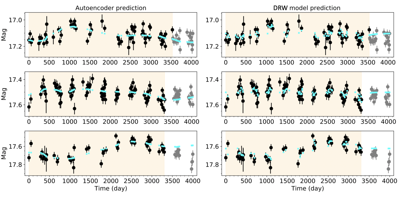
Fig. 7 shows examples of the output of the autoencoder. We compare the modeling part and the forecasting part of the autoencoder and the DRW process for the same objects in the left three panels and the right three panels, respectively. The most apparent difference between them is the scatter in short-timescale variability in the modeling part: the output of the autoencoder is relatively smoother. Short timescale scatter is not resolvable in our data due to the sampling cadence and statistical errors. The DRW process, however, includes short-time variability () to express the overall variance of the light curve (). In other words, the power law index of the PSD of the DRW process must be above the typical frequency, even if the Fourier power is dominated by noise. The autoencoder, on the other hand, models the quasar temporal behavior purely based on the characteristics of the data without any prior assumptions. The suppression of such short-time variability in the autoencoder’s modeling corresponds to a steeper spectral index of the PSD than that of the DRW process in the high frequency regime.
For the forecasting part, the autoencoder seems to output real variations, i.e., the output does not fall to the mean value or diverge upward or downward immediately. The autoencoder also predicts different behavior to the DRW process. We define the prediction of the DRW process as the expectation value from the last data in the modeling part:
| (10) |
where and are the DRW process parameters derived from fitting the process to the modeling part of the light curve, and the is the last observation time in the modeling part.

To assess the forecasting accuracy of the autoencoder model (AE model), we calculated the difference between the reduced chi-square for the AE model and the DRW model for quasar light curves. The blue points in Fig. 8 show for quasar light curves as a function of , where the error bars show the 68% confidence intervals evaluated from bootstrap sampling. The improvement in the forecasting accuracy compared to the DRW model grows roughly as the time separation from the last observation of the modeling part () increases. Hence, at any time separation within days, the AE model performs better than the DRW model in forecasting quasar light curves.
In addition, the autoencoder trained on quasar light curves can capture the characteristics of the DRW process. The green squares in Fig. 8 show the forecasting accuracy of the AE model compared to the DRW model for the simulated light curves. The value of for simulated light curves is close to zero at any . This result should be related to the fact that the autoencoder can recover the value of in the DRW process from simulated light curves as well as a fitted DRW process. This is impressive as it means the autoencoder succeeds in capturing the deterministic term in the DRW process, i.e., the exponential kernel or, at least, suggests that there is an autoregressive nature to quasar variability. It is the deviations in the underlying process(es) from an DRW model that makes the accuracy of forecasting by the AE model better than that of the DRW model.
III.3 Visualizing the AE Features

To understand what the autoencoder identifies in the quasar light curves, we have investigated the characteristics of the AE features. Using principal component analysis (PCA), the distribution of the 16 AE features can be projected onto the plane formed by the first two principal components (Dim1 and Dim2 respectively) as shown in the left panel in Fig. 9. There are three peaks in this distribution at , , and respectively. To see what these prominent features correspond to, we divide the distribution into a grid labelled A–Y, and generate “average” light curves at each grid point using the decoder part of the autoencoder and an input of the averaged 16 AE features at that point. The resulting light curves are displayed in the right panel in Fig. 9. As expected, the averaged light curves at L, Q, and O, which roughly correspond to the peaks in the PDF, show the most global trends of temporal variability: namely stable, brightening, and fading, respectively. If one were to consider a polynomial expansion of the light curve, the three trends would be distinguishable by their primary factor, and these are the most apparent and fundamental characteristics of temporal variability.
On the other hand, some light curves show prominent variation over relatively short timescales, especially in low density regions (e.g., E, U, and Y). The shapes of such average light curves are not simple; they do not show a monotonic brightening/fading and their timescales/amplitudes are not symmetric. We may thus infer that useful information for deriving physical parameters is not associated with simple characteristics, such as the global trend of a light curve, as is the case with high-order coefficients in a polynomial expansion. However, this also shows that most quasar light curves, lying in the denser regions, do not show such prominent variation within the observation baseline ( 4,000 days). This presents a difficulty for deriving the variability timescale of quasars, since, qualitatively, the light curve must show at least a brightening or fading and subsequently go back to its mean value to estimate the time scale of the variation.
III.4 Information Content in Physical Parameters

The relationship between the AE features and physical parameters should be nonlinear. This means that the simple (partial) correlation coefficient or the coefficient of determination cannot be used directly to evaluate the information content between them. However, a multilayer perceptron (MLP) with hidden layers can transform input in a nonlinear way, and should exploit any information in the input associated with the physical parameter in question. We constructed a simple MLP with one hidden layer, and trained it to maximize the value between its output and a given physical parameter. The MLP that we used is shown in Fig. 10. We employed the Adam optimizer with a learning rate of , and also stopped the training when the validation loss had increased with . The mean value and the uncertainty (1) in the information content were computed with 10-fold cross-validation.1212 12 In k-fold CV, 1/k of the training set is withheld during model construction, and the remaining 11/k fraction of the training set is used to predict the of the withheld data. This procedure is repeated k times, with every training set source being withheld exactly once, so that predictions are made for each source in the training set. In addition, we determined the relevance of the AE features to a physical parameter with the following procedure: (1) train the MLP using all 16 AE features to maximize with the physical parameter, (2) feed the true values of one AE feature that we are interested in and zeros to the other nodes, (3) calculate , and (4) repeat this calculation (return to (2)) for each AE feature. This can be understood as the contribution of each AE feature to the coefficient of determination for a specific physical parameter, and thus can be interpreted as the relevance of it to the physical parameter under consideration.
III.4.1 Redshift
In an observed light curve, the intrinsic (restframe) variation timescale is multiplied by so we should expect a correlation between the observed variation timescale and redshift. Kozłowski 2017 has shown that previous reports of an anticorrelation between the variation timescale and the redshift are an artifact of insufficient temporal coverage and that any true correlation has yet to be verified.

The top panel in Fig. 11 shows the importance of the 16 AE features with respect to redshift with Feature 13 (F13) having the highest importance. To see how this feature affects the modeled light curve, we select a fiducial object, CRTS J110718.8100417, whose F13 value is close to its mean value,1313 13 We also selected this object as there is clear brightening and fading in it and therefore the effect of changing AE feature values is more evident. and vary this by . The corresponding changes in the modeled light curve are shown in the bottom panel in Fig. 11. We see that the most significant change is the timescale of the variation, which is precisely what we would expect, but is also the first time that such a change has been demonstrated in quasar light curves. We note that although we have used a single object for illustrative purposes, these trends are seen in the larger statistical sample.
The variability timescale for this source (at ) seems longer than the 245 day limit below which it can be accurately estimated for a DRW model fit. Despite a lack of a quantitative measure, though, the AE feature (F13) controlling the timescale of variability has a relationship with redshift. The coefficient of determination with redshift is (corresponding to the correlation coefficient ) implying that quasar flux variation can explain 7% of the variance in the redshift, or in other words, the quasar light curve has 7% of information content on redshift.
III.4.2 Optical luminosity


Observational biases mean that the optical luminosity, , is strongly dependent on redshift and this needs to be accounted for. Fig. 12 shows the scatter matrix between six parameters for the data set and it can be seen that the correlation between and redshift is strongly nonlinear. We cannot, therefore, disentangle the effect of redshift on the relation between the AE features and with either multiple linear regression analysis or the partial correlation coefficient; instead, we include the redshift as an additional input to the MLP alongside the AE features. AE features known to correlate with redshift, such as Feature 13 or Feature 10, should lose their importance and other features containing information on should emerge as more relevant.
The top panel in Fig. 13 shows the importance, , of the AE features for . As expected, Feature 13 and Feature 10 have lost their relevance and, instead, the most important feature for is Feature 14 (F14). The dependence of the modeled light curve on F14 is shown in the bottom panel in Fig. 13, where the feature value is varied by to around its original value. The modeled light curve changes in only its brightening phase as the feature varies which suggests that the brightening timescale or the asymmetry of the timescale of brightening and fading relates to the luminosity of a quasar. As shown in Fig. 14, the output value increases as the input value to the node corresponding to F14 increases. It suggests a longer brightening timescale, or a higher symmetry, is possibly associated with a higher optical luminosity and that faint quasars might tend to exhibit higher variability asymmetry and vice versa for brighter quasars.
This could indicate different physical mechanisms determining the timescale of brightening and fading. We note that standard second-order analysis techniques, such as the power spectrum density, structure function, or correlation function, are not sensitive to this and neither is the DRW model. The autoencoder models the light curve itself without any prior assumptions and so can capture information on asymmetry if it is present.
The coefficient of determination obtained with the AE features and redshift as input is and with only the redshift is , respectively, giving . Since the increment of the coefficient of determination can be understood as the lower limit of between the AE features and , the flux variations in quasars have information on .
III.4.3 Black hole mass

Fig. 12 shows that the black hole mass, , correlates with redshift and , although the redshift dependency is most likely due to the strong correlation with . We therefore include both and redshift as MLP inputs to handle these relationships. The importance for is shown in the top panel in Fig. 15 with Feature 5 (F5) emerging as the most relevant and its effect on the modeled light curve is presented in the bottom panel in Fig. 15. Asymmetry in the timescale of the brightening and fading is controlled by this feature but in a different way to Feature 14 (see above). Since the correlation coefficient between F5 and is negative (), the asymmetry increases as decreases, and this is consistent with the relation between the AE features and where the asymmetry increases as decreases.
The coefficient of determination with inputs of AE features, redshift, and is and with only redshift and , is , respectively, giving . Again, the flux variations in quasars have information on because can be understood as the lower limit of between the AE features and , as mentioned in §III.4.2. If we regard as the square of the correlation coefficient, we can derive the partial correlation coefficient of the AE features with redshift, luminosity, and black hole mass. The highest partial correlation coefficient is then with luminosity ( 0.1) suggesting that the AE features mainly capture characteristic variability related to luminosity and that correlations with the other parameters might just an artifact of this relationship.
III.5 Asymmetry in quasar light curves
The above results suggest that the timescales of brightening and fading in a quasar light curve are determined by different physical mechanisms, and that the ratio between these two components, i.e., the temporal asymmetry of the curve, is related to . If this is the case then an autoencoder trained on quasar light curves would work a different way for time-inverted (T-inverted) and magnitude-inverted (M-inverted) light curves. An example of the T-inverted and the M-inverted light curve is shown in Fig. 16.
We define the normalized modeling accuracy as: , where
| (11) |
This value is related to the coefficient of determination. Fig. 17 shows the normalized modeling accuracy for quasar light curves and simulated (DRW) light curves, respectively, and in each panel, the normalized accuracy for the original, the T-inverted, and the M-inverted curves is displayed as a function of time in the restframe.
The normalized modeling accuracies for the simulated light curves are almost the same among the three data, whereas those for the quasar light curves show different behavior. The largest deviation from the accuracy of the original quasar light curve comes from the T-inverted light curve; the accuracy for the T-inverted dataset is lower than that of the original dataset during the first half ( 0–600 days), and then improves to higher than that of the original dataset after 700 days. On the other hand, the accuracy for the M-inverted data begins to slightly lag the original dataset at 500 days, and never goes to higher than that of the original dataset. The deviation from the original dataset is smaller than for the T-inverted dataset. As this behavior is not seen in the accuracies for the simulated light curves, it is a characteristic of the quasar light curves and not any observational bias.
No difference in the accuracies for the three datasets of the simulated light curves is actually expected, in fact, because the kernel in the DRW process, , is time-reversible and also brightness reversible; in other words, both the T-inverted DRW process and the M-inverted DRW process are still DRW processes. The difference in the quasar light curves thus suggests variability asymmetry is present, which is consistent with the results in §III.4.2 and §III.4.3, indicating the existence of the arrow of time in these time series. It is indicative that the larger discrepancy is in the accuracy for the T-inverted dataset rather than for the M-inverted dataset. The amplitude of the variability asymmetry is possibly small in terms of magnitude while significant in terms of time.
We note that the modeling accuracy is always larger for the quasar light curves than for the simulated light curves. This is probably because the autoencoder is trained only with the quasar light curves but it also indicates that the quasar flux behavior is different from the DRW process as the parameter estimation by the DRW process fit is not precise. Again, the consistency in the accuracy curves for the three simulated datasets confirms that the discrepancy among the accuracies for the quasar datasets is not attributable to systematic effects such as the amount of data in each bin or seasonal observation gaps.
III.6 Variability Asymmetry analysis
The results from the autoencoder model suggest the existence of variability asymmetry in the quasar light curves. Kawaguchi et al. 1998 introduced a structure function approach to estimate the variability asymmetry adopting two structure functions, and , which only include pair epochs with brightening and fading flux, respectively (i.e., increasing and decreasing flux). The asymmetry can be quantified via an asymmetry parameter :
| (12) |
where “tot” refers to the total set of data pairs. quantifies the normalized difference between the brightening and fading: positive indicates that the light curve favors a rapid rise and gradual decay, and vice versa for a negative . Attributing quasar optical variability to instabilities in the accretion disk (the disk instability model) produces , while the starburst model, which associates variability with the random superposition of supernovae in the starburst region of the host galaxy, yields . Hawkins 2002 also considered gravitational microlensing as a mechanism for variability and demonstrated is expected in this case.
From a sample of 401 quasars, Hawkins 2002 found no asymmetry signature was detected on timescales of a year or longer. However, Giveon et al. 1999 calculated the difference between the medians of brightening phases and fading phases in the light curves of 42 PG quasars and found a negative asymmetry in the variations. More recently, significant negative asymmetry was detected on a timescale longer than 300 days in 7,562 quasars from SDSS Stripe 82 (Voevodkin 2011).
Fig. 18 shows the ensemble for the quasar light curves and the simulated light curves. To obtain the ensemble , we calculated for all sources in the quasar dataset, and then estimated using the weighted average in 10-day width bins. Since the DRW process is variability symmetric the ensemble for the simulated light curves does not show any significant deviation from . However, the ensemble for the quasar light curves, presented in the top panel in Fig. 18, has positive on short timescales, and then decreases to a statistically significant negative value for days. This behavior indicates that the brightening power of variability is stronger than the fading power on a timescale shorter than days, while vice versa on a timescale longer than days. The variability asymmetry, which is suggested by the deep learning modeling, is confirmed by this time domain analysis.
We note that our quasar sample has been selected to only consist of spectroscopically-confirmed sources and that a variance-luminosity relation has been employed so that variability is solely from the accretion disk. Additionally, the sample size is about double that used by Voevodkin 2011, and the observation cadence is much denser than that of the SDSS Stripe 82 dataset. Our result is therefore the most definitive to date.
IV Discussion
IV.1 The autoencoder model and its features
The autoencoder (AE) model we have trained on quasar light curves provides a better description of quasar optical variability than the damped random walk (DRW) model commonly used in the literature. In particular, the forecasting accuracy of the AE model relative to the DRW model improves as increases suggesting that the AE model captures characteristics of the long-term behavior in quasar light curves. Quasar variability on timescales longer than several hundred days has not been well determined so far, partly due to insufficient data sets, but also as characteristic timescales from the DRW model are biased low for time series with temporal coverage less than ten times the timescale in question. Caplar et al. 2017 found that there are clear variations in the slopes of the quasar structure function (SF) for individual sources with many quasars having steeper SFs than expected from the DRW model. Quasars with higher mass and/or luminosity tend to have steeper power spectral density (PSD) slopes and this can be reproduced in a model where the PSD slope is steeper below a certain timescale which is dependent on mass and/or luminosity. This may be the same behavior that the AE model is capturing.
The AE model is trained to reproduce all of the light curves with only 16 parameters for each object. Simple clustering analysis of the AE features shows three populations: fading, stable, and brightening, which agrees with the most intuitive categorization. However, mean light curves across the grid-separated PCA projection of the features show highly flexible expressions including global trend, variable amplitude, variable timescale, etc. This shows that the AE features have most of the latent content of the variability but this is also tied to physical parameters since the information content on the luminosity is seen to increase as training proceeds and the distributions of some physical parameters on the PCA map show correlations. This implies that the shapes of stochastic time series contain information on the physical properties and processes producing them.
In fact, we have specifically used the AE features in deep regression models for redshift, black hole mass, and luminosity. If the intrinsic variability is redshift independent then the observed frame light curves should show a relation between the timescale of variability and redshift (or strictly ). We find that AE feature 13 which controls the visual timescale of variability is the most relevant feature in determining redshift which validates our approach. It is perhaps more surprising, though, that an AE feature which controls visual asymmetry in the light curve should also be the most relevant for both luminosity and black hole mass. This suggests for the first time that the degree of asymmetry in quasars should be higher for low luminosity (black hole mass) systems which are also known to show higher amplitude variability.
IV.2 Variability asymmetry in quasar light curves
Variability asymmetry is confirmed to be more than just a visual effect by the AE modeling and forecasting accuracies for time-inverted (T-inverted) and magnitude-inverted (M-inverted) light curves, i.e., the autoencoder performs differently for the original, the M-inverted, and the T-inverted data sets. Interestingly, accuracies for the T-inverted curves are higher than those for the original curves in some temporal regions, while those for the M-inverted curves are always lower than those of the original data set. However, as expected, these asymmetries are not seen in simulated light curves generated by the (time reversible) DRW process.
A more traditional time domain analysis based on the structure function also finds variability asymmetry, demonstrating that it is not an artifact of the deep learning approach. The SF asymmetry parameter indicates that on shorter timescales ( days) there is a shorter brightening phase with a longer fade while the reverse is seen on longer timescales ( days). This trend is also consistent with the result obtained from MLP regression between the AE features and physical parameters where the variability asymmetry emerges in the form of a shorter brightening phase with a longer fading phase.
We have seen as well that the variability asymmetry is connected to the intrinsic luminosity of quasars. Theoretical predictions for this behavior are scant in the literature but the most plausible physical model matching our results is the disk instability model (Takeuchi et al. 1995; DI model hereafter) based on the concept of self-organized criticality (Bak et al. 1988). In this model, mass accretion takes place in the form of avalanches which occur only when the local mass density exceeds a critical value, and, simultaneously, a gradual viscous diffusion occurs regardless of the critical condition. The DI model has so far been mainly applied to X-ray variability in stellar mass black holes but it seems applicable to quasars with black holes a factor of larger. Simulated light curves generated by this process, e.g., Takeuchi et al. 1995, Kawaguchi et al. 1998, show variability asymmetry of or , depending on the avalanche rate, the ratio of the diffusion mass, , to the accretion mass, , and the range of the radius of the accretion disk that we are interested in. Kawaguchi et al. 1998 demonstrated that simulated optical light curves of quasars exhibit a negative asymmetry on time scales of several hundred days in the rest frame which is consistent with our results. Specifically they found that is obtained with the ratio of the diffusion mass to inflow mass of 0.1–0.5.
We can also consider the relation between variability asymmetry and luminosity within the context of this model. The ratio of the diffusion mass to the accretion mass controls the variability asymmetry and so at a lower value, , the variability asymmetry is relatively large, at days, but at a higher value, , the asymmetry is effectively suppressed. So luminous quasars should intrinsically have a high ratio of to while less luminous quasars should have a relatively smaller value. The amplitude of variability is also suppressed by a high diffusion mass ratio in the DI model because large amplitude variability comes from large-scale avalanches and these hardly occur when mass diffusion is efficient. Thus a natural consequence of this is that the amplitude of variability is anticorrelated with luminosity as has been found in several analyses.
The diffusion (or viscous) timescale for an accretion disk, , gives the characteristic timescale of mass flow and can be parameterized for a black hole of mass at (Stern et al. 2018) as:
| (13) |
where is the disk viscosity parameter, is the disk aspect ratio, is the disk radius, and is the gravitational radius. should be inversely proportional to the amount of diffusion mass, , per unit time and so , which should be higher for luminous quasars. As both the amount of diffusion mass and the inflow mass per unit time should increase simultaneously as increases, the ratio should be fairly independent of . The scale height, , would thus be the most plausible physical parameter responsible for differences in the variability asymmetry in the standard disk regime.
One possible explanation is that quasars with higher metallicity (based on the measured metallicity of the broad line regions) appear to have systematically smaller continuum reverberation lags, i.e., smaller disk sizes. Jiang et al. 2017 found that high-luminosity quasars seem to follow a disk temperature profile, , with , which is also confirmed by microlensing (Blackburne et al. 2011; Hall et al. 2014). If high-luminosity quasars have a high volume of metallicity resulting in a small emission region for the optical band, then a larger scale height, , can be expected for a fixed height disk at radius . In fact, a relation between black hole mass and quasar metallicity has already been suggested, e.g., Warner et al. 2003; Kisaka et al. 2008. The relationship between disk size and metallicity may result in large changes in disk opacity as a function of the gas metallicity, which can significantly alter the thermal properties and structure of the accretion disk. This might then explain the connection between variability asymmetry and luminosity. Alternatively, a large mass accretion rate can also be responsible for a large scale height as it should lead to a large amount of photon emission from the disk and also a large surface density. The gas pressure at the radius exhibiting a fixed temperature should thus be relatively larger for luminous quasars, and, as the gas pressure contributes to the scale height. luminous quasars should have accretion disks with a relatively larger scale height.
However, our variability asymmetry is positive, , on a short timescale ( days) and the opposite on longer timescales ( days). A single physical mechanism may be responsible for variability asymmetry on all timescales or different mechanisms may produce it on the short and longer timescales respectively. Takeuchi et al. 1995 showed that simulated and observed X-ray fluctuations at a radius of exhibit positive variability asymmetry, which supports a single mechanism, but the simulations of Kawaguchi et al. 1998 consider a different radius range. As the disk temperature decreases proportional to , the radius range emitting higher energy photons should be smaller relative to that producing lower energy photons which might mean that short timescale fluctuations from the smaller region show the positive variability asymmetry and vice versa for the longer timescale fluctuations. The starburst model, which attributes aperiodic luminosity variations to the random superposition of supernovae in the nuclear region, would be consistent with this and Kawaguchi et al. 1998 demonstrated that it produces significant positive asymmetry on a timescale of 1–100 days in agreement with our results. Additionally, a high supernova rate implies larger luminosity quasars and lower variability amplitude. This model cannot, however, explain the negative asymmetry seen and so another process must be responsible for the transition seen from positive to negative asymmetry as the variation timescale increases.
It is possible that the variability seen is not the direct product of a single intrinsic process but a convolution of several. The optical flux of quasars must contain broad line emissions which are thought to be produced light days from the central region (e.g., Peterson 1997). Although the contribution to the total flux is only of order a few percent, it is detectable in statistical measures of variability, such as the autocorrelation function. 1 – 50 day continuum reverberation lags in the UV-optical bands have also been measured in several local AGN, e.g., NGC 4395, NGC 4593, NGC 5548, and NGC 4151 (see McHardy et al. 2018 and references therein). Light curves with contributions from both phenomena can be produced by convolving the underlying process with an appropriate kernel and Fig. 19 shows three example kernel functions and their PSDs. In principle, any kernel will reduce high-frequency power, resulting in a steeper PSD spectral index than the original1414 14 The PSD of convolved time-series can be calculated by , where is the original PSD and is the PSD of the kernel function. .
Fig. 20 shows an example of the PSD of the DRW process convolved with a kernel. At frequencies above the typical timescale of the kernel function, the PSD shows a steeper spectral index ( with this kernel) than that of the original PSD ( for the DRW process). We can thus expect at least two breaks in the PSD when convolved with a kernel function with steepened spectral indices as the frequency increases. The light curve from the convolved process should also show a higher correlation coefficient than that of the original temporal flux variation and the correlation should have a duration roughly corresponding to the typical timescale of the kernel. The observed quasar PSD slope is significantly steeper than on timescales shorter than month [REF]. Kernel convolution naturally generates the steeper PSD slope above the typical timescale of the kernel, which should itself correlate with black hole mass and/or quasar luminosity, resulting from the scaling law with . This suggests that assuming that quasar flux variation contains some amount of reverberated flux can explain the complex behavior of the time variation and also the PSD characteristics revealed so far. The existence of a kernel function, which manifests as the timescale with a high correlation coefficient in the quasar variation, also possibly explains the higher modeling/forecasting accuracy of the autoencoder model for the T-inverted data set than that for the original data set.
V Summary and Conclusions
We have constructed a nonparametric model to describe the optical variability of quasars with a small number of representative features using a recurrent autoencoder (AE), a type of deep neural network suited for time series (sequential) data. The AE has been trained to both model (predict) and forecast quasar behavior by using truncated time series (by 500 days) as input and minimizing the reduced chi squared between the output of the network and the original full light curve. With real data, it provides a more accurate forecast than the corresponding damped random walk (DRW) model fit to the input and the AE performance improves relative to the DRW model with increasing forecasting time. With simulated light curves from a DRW process, however, both models show comparable accuracy and this demonstrates that the trained AE can capture properties in the DRW process and, indeed, recover DRW process parameters. It also shows that quasar variability differs from a DRW model.
The AE also provides a compact learned representation of the input data set (and thus quasar variability) via the encoded features from the most compressed hidden layer. These enable investigations of the relations between the temporal flux variation of quasars and their physical parameters, specifically redshift, luminosity, and black hole mass. To simplify this, we trained a multilayer perceptron (MLP) model on the AE features to maximize the coefficient of determination () between the respective physical parameter and the output of the MLP. The importance of each AE feature was also evaluated based on its effect in improving . The feature responsible for the timescale of variability was found to be the most relevant for redshift, as expected; however, we also identified the feature controlling variability asymmetry as the most important for predicting luminosity and black hole mass.
The existence of variability asymmetry is shown by different model/forecasting accuracies for time-inverted (T-inverted) and magnitude-inverted (M-inverted) versions of the input data set. This is not seen when dealing with simulated time series from a DRW process which is naturally time symmetric. The AE fit to the T-inverted data set shows a higher forecasting accuracy than the original dataset over a limited time range and this implies that the T-inverted light curves have information on future variability which equates to past variability in the original data set. Independent analysis of the same data sets using the structure function confirms a variability asymmetry connected with optical luminosity and black hole mass and that the hysteresis in the variability differs from a DRW process. A positive variability asymmetry is present on short timescales ( days) and a negative asymmetry on longer timescales ( days).
The observed asymmetry is consistent with the disk instability (DI) model where variability from the accretion disk is ascribed to instabilities in the disk as matter flows and the asymmetry to large-scale avalanches. Light curves generated from Monte Carlo simulations of this behavior show a positive asymmetry in variability from a compact inner region close to the central black hole while a negative asymmetry in the variability emerges from a wide outer region (Takeuchi et al. 1995; Kawaguchi et al. 1998). CRTS is an unfiltered survey and therefore sensitive from NIR to UV wavelengths so the observed temporal flux variations should contain those originating over a wide range of the accretion disk. Given the disk temperature profile as a function of radius, , fast variability should come from the inner compact region, possibly generating the positive asymmetry, and vice versa for longer timescale variability.
The magnitude of the variability asymmetry is controlled by the ratio of the diffusion mass to the inflow mass with the asymmetry diminishing as the ratio increases. We found that the asymmetry decreases as the luminosity increases which requires efficient mass diffusion in the accretion disks of luminous quasars. This can be interpreted in light of prior observational results that quasars with higher metallicity have smaller disk sizes at a fixed wavelength and also that black hole mass seems to correlate with metallicity. If we can assume that the height of the disk is determined by the mass accretion rate at a radius and that the dispersion of the mass accretion rate is small among quasars, then luminous quasars should have a relatively smaller disk and larger scale height () at a portion of the accretion disk with fixed disk temperature. Alternatively, the high accretion mass rate could be responsible for a higher accretion disk scale height in luminous quasars. As the scale height is proportional to the diffusion mass rate, luminous quasars should have lower variability asymmetry with lower variability amplitude as the efficient mass diffusion results in fewer large avalanches. This is consistent with previous results in the literature that luminous quasars exhibit lower amplitude variability.
The AE fit to the T-inverted data set shows a lower modeling/forecasting accuracy over particular timescales. A natural interpretation is that quasar variability retains information from prior activity over certain time frames. This can be represented mathematically by treating an observed time series as the convolution of an intrinsic time series and a kernel function. Contributions from reverberation at the broad line region and/or from the accretion disk itself must be present in the quasar flux variation and these typically show 10 – 100 day time lags relative to the intrinsic flux variability and so are a predictable component with such timescales. The kernel function can also address the discrepancy from the DRW process in the quasar PSD: the slope of the PSD gets steeper on shorter timescales and the slope seems to correlate with luminosity and/or black hole mass. The kernel convolution significantly reduces variability on a timescale shorter than that of the kernel function, and the typical timescale should scale with black hole mass.
Finally, the next generation time domain surveys, such as the Zwicky Transient Facility (ZTF; Bellm et al. 2019; Graham et al. 2019) and the Vera Rubin Observatory (LSST Science Collaboration et al. 2009), will provide multicolor observations with only a few night’s cadence over several years for millions of quasars. This will greatly improve our ability to test and assess explanations of quasar physics; for example, our model for quasar variability suggests different variation characteristics in different energy bands. The disk instability model predicts that bluer color on a short timescale variability changes to redder color on longer timescales and the negative variability asymmetry on longer timescales should be smaller in higher energy bands. It is also interesting to consider what an autoencoder trained on multicolor higher cadence photometric observations might show. Physical labels from spectra, such as the equivalent width of an emission line or the strength ratio of certain emission lines, can be mapped to the projected distribution of autoencoder features provided by PCA or other dimensional reduction techniques, such as T-SNE or UMAP. This would provide a novel picture clearly relating spectroscopic properties to variability characteristics.
Acknowledgements
This work was supported in part by the NSF grants AST-1518308, and AST-1815034, and the NASA grant 16-ADAP16-0232. The work of DS was carried out at Jet Propulsion Laboratory, California Institute of Technology, under a contract with NASA.
YT was funded by JSPS KAKENHI Grant Numbers JP16J05742. YT studied as a Global Relay of Observatories Watching Transients Happen (GROWTH) intern at Caltech during the summer and fall of 2017. GROWTH is funded by the National Science Foundation under Partnerships for International Research and Education Grant No 1545949.
NK acknowledges the support by MEXT Kakenhi Grant number 17H06362 and the JPSP PIRE program.
References
- Aguado et al. (2019) Aguado, D. S., Ahumada, R., Almeida, A., et al. 2019, ApJS, 240, 23
- Andrae et al. (2013) Andrae, R., Kim, D.-W., & Bailer-Jones, C. A. L. 2013, Astronomy & Astrophysics, 554, A137
- Aretxaga et al. (1997) Aretxaga, I., Cid Fernandes, R., & Terlevich, R. J. 1997, MNRAS, 286, 271
- Assef et al. (2018) Assef, R. J., Prieto, J. L., Stern, D., et al. 2018, ApJ, 866, 26
- Bak et al. (1988) Bak, P., Tang, C., & Wiesenfeld, K. 1988, Physical Review A (General Physics), 38, 364
- Becker et al. (2020) Becker, I., Pichara, K., Catelan, M., et al. 2020, MNRAS, 322
- Bellm et al. (2019) Bellm, E. C., Kulkarni, S. R., Graham, M. J., et al. 2019, PASP, 131, 018002
- Blackburne et al. (2011) Blackburne, J. A., Pooley, D., Rappaport, S., & Schechter, P. L. 2011, The Astrophysical Journal, 729, 34
- Bruce et al. (2016) Bruce, V. A., Dunlop, J. S., Mortlock, A., et al. 2016, MNRAS, 458, 2391
- Caplar et al. (2017) Caplar, N., Lilly, S. J., & Trakhtenbrot, B. 2017, The Astrophysical Journal, 834, 111
- Charnock & Moss (2017) Charnock, T., & Moss, A. 2017, ApJ, 837, L28
- Drake et al. (2009) Drake, A. J., Djorgovski, S. G., Mahabal, A., et al. 2009, ApJ, 696, 870
- Drake et al. (2011) —. 2011, ApJ, 735, 106
- Drake et al. (2013) Drake, A. J., Catelan, M., Djorgovski, S. G., et al. 2013, The Astrophysical Journal, 763, 32
- Drake et al. (2014) Drake, A. J., Graham, M. J., Djorgovski, S. G., et al. 2014, The Astrophysical Journal Supplement Series, 213, 9
- Giveon et al. (1999) Giveon, U., Maoz, D., Kaspi, S., Netzer, H., & Smith, P. S. 1999, Monthly Notices of the Royal Astronomical Society, 306, 637
- Graham et al. (2014) Graham, M. J., Djorgovski, S. G., Drake, A. J., et al. 2014, Monthly Notices of the Royal Astronomical Society, 439, 703
- Graham et al. (2017a) —. 2017a, Monthly Notices of the Royal Astronomical Society, 470, 4112
- Graham et al. (2017b) —. 2017b, MNRAS, 470, 4112
- Graham et al. (2015) Graham, M. J., Djorgovski, S. G., Stern, D., et al. 2015, Monthly Notices of the Royal Astronomical Society, 453, 1562
- Graham et al. (2019) Graham, M. J., Kulkarni, S. R., Bellm, E. C., et al. 2019, PASP, 131, 078001
- Guo et al. (2017) Guo, H., Wang, J., Cai, Z., & Sun, M. 2017, The Astrophysical Journal, 847, 132
- Hall et al. (2014) Hall, P. B., Noordeh, E. S., Chajet, L. S., Weiss, E., & Nixon, C. J. 2014, Monthly Notices of the Royal Astronomical Society, 442, 1090
- Hawkins (1993) Hawkins, M. R. S. 1993, Nature, 366, 242
- Hawkins (2002) —. 2002, Monthly Notices of the Royal Astronomical Society, 329, 76
- Hawkins (2010) —. 2010, MNRAS, 405, 1940
- Jain & Medsker (1999) Jain, L. C., & Medsker, L. R. 1999, Recurrent Neural Networks: Design and Applications, 1st edn. (Boca Raton, FL, USA: CRC Press, Inc.)
- Jarosik et al. (2011) Jarosik, N., Bennett, C. L., Dunkley, J., et al. 2011, The Astrophysical Journal Supplement, 192, 14
- Jiang et al. (2017) Jiang, Y.-F., Green, P. J., Greene, J. E., et al. 2017, The Astrophysical Journal, 836, 186
- Kasliwal et al. (2015) Kasliwal, V. P., Vogeley, M. S., & Richards, G. T. 2015, Monthly Notices of the Royal Astronomical Society, 451, 4328
- Kawaguchi et al. (1998) Kawaguchi, T., Mineshige, S., Umemura, M., & Turner, E. L. 1998, The Astrophysical Journal, 504, 671
- Kelly et al. (2009) Kelly, B. C., Bechtold, J., & Siemiginowska, A. 2009, The Astrophysical Journal, 698, 895
- Kelly et al. (2011) Kelly, B. C., Sobolewska, M., & Siemiginowska, A. 2011, The Astrophysical Journal, 730, 52
- King et al. (2004) King, A. R., Pringle, J. E., West, R. G., & Livio, M. 2004, MNRAS, 348, 111
- Kingma & Ba (2014) Kingma, D. P., & Ba, J. 2014, ArXiv e-prints, arXiv:1412.6980
- Kisaka et al. (2008) Kisaka, S., Kojima, Y., & Otani, Y. 2008, Monthly Notices of the Royal Astronomical Society, 390, 814
- Kozłowski (2017) Kozłowski, S. 2017, Astronomy & Astrophysics, 597, A128
- Lawrence et al. (2016) Lawrence, A., Bruce, A. G., MacLeod, C., et al. 2016, MNRAS, 463, 296
- Lipton et al. (2015) Lipton, Z. C., Berkowitz, J., & Elkan, C. 2015, arXiv e-prints, arXiv:1506.00019
- LSST Science Collaboration et al. (2009) LSST Science Collaboration, Abell, P. A., Allison, J., et al. 2009, arXiv e-prints, arXiv:0912.0201
- MacLeod et al. (2012) MacLeod, C. L., Ivezić, Ž., Sesar, B., et al. 2012, The Astrophysical Journal, 753, 106
- Mahabal et al. (2011) Mahabal, A. A., Djorgovski, S. G., Drake, A. J., et al. 2011, Bulletin of the Astronomical Society of India, 39, 387
- McHardy et al. (2018) McHardy, I. M., Connolly, S. D., Horne, K., et al. 2018, Monthly Notices of the Royal Astronomical Society, 480, 2881
- Meusinger et al. (2010) Meusinger, H., Henze, M., Birkle, K., et al. 2010, A&A, 512, A1
- Morganson et al. (2014) Morganson, E., Burgett, W. S., Chambers, K. C., et al. 2014, The Astrophysical Journal, 784, 92
- Mushotzky et al. (2011) Mushotzky, R. F., Edelson, R., Baumgartner, W., & Gandhi, P. 2011, The Astrophysical Journal Letters, 743, L12
- Naul et al. (2018) Naul, B., Bloom, J. S., Pérez, F., & van der Walt, S. 2018, Nature Astronomy, 2, 151
- O’Donnell (1994) O’Donnell, J. E. 1994, Astrophysical Journal, 422, 158
- Palaversa et al. (2013) Palaversa, L., Ivezić, Ž., Eyer, L., et al. 2013, The Astronomical Journal, 146, 101
- Peterson (1997) Peterson, B. M. 1997, An Introduction to Active Galactic Nuclei
- Ross et al. (2018) Ross, N. P., Ford, K. E. S., Graham, M., et al. 2018, MNRAS, 480, 4468
- Ruan et al. (2016) Ruan, J. J., Anderson, S. F., Cales, S. L., et al. 2016, ApJ, 826, 188
- Stern et al. (2018) Stern, D., McKernan, B., Graham, M. J., et al. 2018, ApJ, 864, 27
- Suberlak et al. (2017) Suberlak, K., Ivezić, Ž., MacLeod, C. L., Graham, M., & Sesar, B. 2017, Monthly Notices of the Royal Astronomical Society, 472, 4870
- Tachibana & Miller (2018) Tachibana, Y., & Miller, A. A. 2018, Publications of the Astronomical Society of the Pacific, 130, 128001. http://stacks.iop.org/1538-3873/130/i=994/a=128001
- Takeuchi et al. (1995) Takeuchi, M., Mineshige, S., & Negoro, H. 1995, Publications of the Astronomical Society of Japan, 47, 617
- Vanden Berk et al. (2004) Vanden Berk, D. E., Wilhite, B. C., Kron, R. G., et al. 2004, The Astrophysical Journal, 601, 692
- Voevodkin (2011) Voevodkin, A. 2011, arXiv e-prints, arXiv:1107.4244
- Warner et al. (2003) Warner, C., Hamann, F., & Dietrich, M. 2003, The Astrophysical Journal, 596, 72
- Wills et al. (1993) Wills, B. J., Brotherton, M. S., Fang, D., Steidel, C. C., & Sargent, W. L. W. 1993, Astrophysical Journal, 415, 563
- Wold et al. (2007) Wold, M., Brotherton, M. S., & Shang, Z. 2007, Monthly Notices of the Royal Astronomical Society, 375, 989
- Zuo et al. (2012) Zuo, W., Wu, X.-B., Liu, Y.-Q., & Jiao, C.-L. 2012, ApJ, 758, 104