Octagon at finite couplingUnité Mixte de Recherche 3681 du CNRSPreprint: IPhT–T20/007
Abstract
We study a special class of four-point correlation functions of infinitely heavy half-BPS operators in planar SYM which admit factorization into a product of two octagon form factors. We demonstrate that these functions satisfy a system of nonlinear integro-differential equations which are powerful enough to fully determine their dependence on the ’t Hooft coupling and two cross ratios. At weak coupling, solution to these equations yields a known series representation of the octagon in terms of ladder integrals. At strong coupling, we develop a systematic expansion of the octagon in the inverse powers of the coupling constant and calculate accompanying expansion coefficients analytically. We examine the strong coupling expansion of the correlation function in various kinematical regions and observe a perfect agreement both with the expected asymptotic behavior dictated by the OPE and with results of numerical evaluation. We find that, surprisingly enough, the strong coupling expansion is Borel summable. Applying the Borel-Padé summation method, we show that the strong coupling expansion correctly describes the correlation function over a wide region of the ’t Hooft coupling.
1 Introduction
In this work, we continue the study of four-point correlation functions of heavy single-trace half-BPS operators in maximally supersymmetric super Yang-Mills theory initiated in Ref. Belitsky:2019fan. It has recently been realized in Refs. Coronado:2018ypq; Coronado:2018cxj that, under a judicial choice of polarizations of half-BPS operators, these correlation functions can be constructed at finite ’t Hooft coupling in terms of a fundamental building block – the octagon . Taking advantage of integrability of the effective two-dimensional worldsheet in the AdS/CFT correspondence, the octagon can be expressed in terms of the hexagon form factors Basso:2015zoa; Fleury:2016ykk; Eden:2016xvg; Bajnok:2017mdf describing dynamics of magnons propagating on the string worldsheet.
At present, explicit expressions for the octagon are known in planar SYM both at weak Coronado:2018ypq; Coronado:2018cxj and strong coupling Bargheer:2019kxb; Bargheer:2019exp. At finite coupling, a concise representation for the octagon as a determinant of a semi-infinite matrix was worked out in Refs. Kostov:2019stn; Kostov:2019auq. This result laid out the foundation for our analysis in Ref. Belitsky:2019fan, where the octagon was further recast as a Fredholm determinant of an integral operator defined on a semi-infinite line. The kernel of the operator in question turned out to be closely related to the Bessel kernel that previously appeared in the study of the Laguerre ensemble in random matrix theory Forrester:1993vtx; Tracy:1993xj.
At weak coupling, the octagon is given by a multilinear combination of the so-called ladder integrals Coronado:2018cxj. The corresponding expansion coefficients can be determined to any loop order by requiring the octagon to have an appropriate asymptotic behavior in different kinematical limits. At strong coupling, for , the octagon possesses a semiclassical asymptotic behavior , where is the minimal area of a string that ends on four geodesics in AdS Bargheer:2019exp; Bargheer:2019kxb.
In this paper, we determine the octagon at finite ’t Hooft coupling. To achieve this goal, we exploit its representation as a Fredholm determinant of a (modified) Bessel kernel. In this formulation, the problem is akin to that encountered in study of two-point functions in integrable low-dimensional theories Korepin:1993kvr. Following a general strategy after Its-Izergin-Korepin-Slavnov Its:1990, we derive a system of exact equations obeyed by the octagon and demonstrate that its solution interpolates between weak and strong coupling expansions. Our consideration adds to a scarce list of examples where correlations functions in an interacting field theory can be determined for arbitrary coupling.
The starting point of our analysis is a four-point correlation function of single-trace half-BPS operators, dubbed the simplest in Ref. Coronado:2018ypq,
| (1) |
where the four operators are built out of two complex scalars and and their complex conjugate partners, , and . Here is a function of the cross ratios
| (2) |
and the coupling constant .
The correlation function (1) is dual to a scattering amplitude of four closed string states. In the limit when the operators become infinitely heavy, for , it factorizes into a double copy of an open-string partition function, the octagon Coronado:2018ypq
| (3) |
Our goal is to find at finite coupling constant and for generic values of the cross ratios.
As a first step in this direction, we can consider the null limit , or equivalently and , when the four operators in (1) are light-like separated in a sequential manner. Introducing convenient kinematical variables and , one finds that in the null limit the octagon takes on a remarkably simple form at weak coupling Coronado:2018cxj; Kostov:2019auq
| (4) |
where the ellipses denote subleading terms which vanish for with fixed and .
The dependence on the coupling constant enters (4) through the two functions and . In our previous study Belitsky:2019fan, we used the aforementioned determinant representation of the octagon to find their exact expressions
| (5) |
Taking the relation (4) at face value and going to the strong coupling limit results in some puzzling consequences. As alluded to above, is expected to have a linear growth in at most. It is easy to see that the first two terms in the right-hand side of (4) do have such a scaling whereas the third term grows as .
The strong coupling limit of the octagon was studied in Ref. Bargheer:2019exp using a clustering technique previously developed in Ref. Jiang:2016ulr in application to three-point correlation functions. In the limit , the octagon takes the form
| (6) |
where is the Euler-Mascheroni constant. Comparing this relation with (4) and (5), we observe that the leading terms coincide at strong coupling. For the second term in Eq. (4), however, the strong coupling limit of yields a result which is twice smaller than that in (6). Finally, the dependent terms in (4) and (6) exhibit different dependence on and . These observations are troublesome, but a priori not completely unexpected since the two results (4) and (6) were obtained in two different regions of the parameter space, for and , respectively. This suggests that the difference between (4) and (6) at strong coupling is due to an order of limits Bargheer:2019exp. We show below that this is indeed the case.
To address this question, we develop a systematically expansion of in powers of for general values of the cross-ratios (2). Doing so, one may attempt to apply the clustering technique Jiang:2016ulr. The method is very efficient for extracting the leading large asymptotics but it generalization to subleading terms suppressed by powers of proves to be difficult. 11 1 The reason being, since the magnon rapidity scaling at strong coupling is not homogeneous, it requires sewing plane-wave and giant magnon regimes through the exact treatment of the near flat space domain. This is doable for a single bound state, but impenetrable for more by brute force. Presently, we demonstrate that these difficulties can be avoided by solving the abovementioned system of exact equations for the octagon at large . We work out its strong coupling expansion in different kinematical limits and compare it with numerical results. We observe that the strong coupling expansion is given by a Borel summable series in . Applying the Borel–Padé summation method, we show that the resulting expression for the octagon agrees with its numerical value over a wide range of the coupling constant.
The paper is organized as follows. In Section 2, we review the representation of the octagon as a determinant of a semi-infinite matrix obtained in Refs. Kostov:2019stn; Kostov:2019auq. We demonstrate that this matrix can significantly be simplified by an appropriate similarity transformation allowing us to express the octagon as a Fredholm determinant of the Bessel kernel modified by some function of the coupling constant and cross ratios. Applying the method of differential equations Its:1990 to this determinant, we derive a system of nonlinear integro-differential equations for the octagon. Its solution at weak coupling is presented in Section 3. In Section 4, we discuss the properties of the octagon at strong coupling and calculate the leading term of its expansion at large . In Section 5, we develop a systematic series of the octagon in the inverse coupling and present analytical expressions for accompanying expansion coefficients. We use these results in Section 6 to study properties of the octagon in different kinematical regimes. In Section 7, we compare the obtained expressions with the numerical results. Section 8 contains concluding remarks. Technical details of our analysis are summarized in four appendices.
2 Octagon as a Fredholm determinant
In this section, we discuss the determinant representation of the octagon and use it to derive a system of exact equations that it obeys.
2.1 Kinematical limits
We will study the octagon in Euclidean and Lorentzian kinematical regimes. Depending on the choice of the region of interest, it is convenient to introduce auxiliary kinematical variables
| (7) |
where . The variables and are real in the Euclidean regime, so that .
The corresponding expressions for the cross ratios (2) are
| (8) |
For future reference, we describe different OPE limits that we examine below in detail.
Euclidean short-distance limit
In this limit, two operators in the correlation function (1) collide and the asymptotics of is controlled by the operators with the lowest scaling dimensions propagating in the corresponding OPE channel. We can distinguish two different OPE limits
| (9) |
corresponding to and , respectively.
In the first case, the leading contribution to the octagon comes from single-trace operators with the scaling dimension and it takes the form . At strong coupling, the anomalous dimension increases with and the octagon is expected to vanish .
In the second case, the OPE is dominated by double-trace operators with the scaling dimension . Their contribution to the octagon scales as and the octagon approaches a finite value .
In what follows we refer to the two limits in (9) as single- and double-trace OPE limits, respectively.
Lorentzian null limit
In this limit, the operators in (1) are located at the vertices of a null rectangle and we have
| (10) |
The leading contribution in each OPE channel comes from single-trace operators with the leading twist and large Lorentz spin. As in the previous case, their anomalous dimension grows indefinitely at strong coupling leading to exponentially small octagon , see Eqs. (4) and (6).
Symmetric point
In this case, we have and in the Euclidean regime. This kinematical configuration does not correspond to a particular OPE limit. The reason why we consider it is that the octagon simplifies and reveals some interesting properties.
2.2 Determinant representation of the octagon
As was mentioned in the Introduction, the octagon at finite coupling admits a representation in terms of a determinant of a semi-infinite matrix Kostov:2019stn; Kostov:2019auq
| (11) |
where is a scalar factor depending on kinematical variables and the matrices and are
| (12) |
where and is a Bessel function. In the hexagonalization approach Basso:2015zoa; Fleury:2016ykk; Eden:2016xvg, the relation (11) comes about as a result of resummation over an arbitrary number of elementary excitations and their bound states propagating on the worldsheet of an open string describing the octagon.
At weak coupling, the representation (11) can be used efficiently to expand in powers of . Since the matrix elements (2.2) scale as , to any given order in we can replace the matrix in (11) by its finite-dimensional minor and expand in powers of . As was shown in Ref. Kostov:2019auq, this leads to the weak-coupling expansion of the octagon in terms of known ladder integrals as was previously bootstrapped in Refs. Coronado:2018ypq; Coronado:2018cxj.
At finite coupling, the calculation of (11) may seem to be problematic due to a rather complicated form of the matrix. This matrix depends in a nontrivial way on the coupling constant and the kinematical variables and encoding the cross ratios (2.1). As we demonstrated in Ref. Belitsky:2019fan, the octagon simplifies significantly for . In this case, the matrix (2.2) reads
| (13) |
where we inserted the subscript to indicate that this relation holds for . Notice that in distinction to (2.2), the matrix elements vanish for even and, as a consequence, the matrix has a block structure. Taking advantage of this property, we were able to recast the octagon (11) at into the form of a Fredholm determinant of a (modified) Bessel kernel Forrester:1993vtx; Tracy:1993xj. We will see momentarily that the octagon admits a similar representation for arbitrary .
2.3 Similarity transformation
Denoting , we observe that the octagon is invariant under a similarity transformation . Choosing appropriately we can simplify the form of the semi-infinite matrix . 22 2 The existence of such transformation was hinted in Ref. Kostov:2019auq.
As a hint, we examine a trace of this matrix, . Replacing with its expression (2.2) we get
| (14) |
where we applied a summation formula for the Bessel functions and changed the integration variable to . Notice that, aside from the factor , the dependence of (14) only resides in the denominator of the integrand. In particular, the dependence of the integrand in (14) on can be restored from its value at by simply replacing in the denominator of (14).
Applying the same recipe to Eq. (13), we define the matrix
| (15) |
By construction, it satisfies the relation . It is a straightforward but tedious exercise to verify that analogous relations holds for powers of the two matrices, with . This suggests that the two matrices and are related to each other by a similarity transformation
| (16) |
We verified that at weak coupling 33 3 Analogous calculation was also performed by Valentina Petkova, we are grateful to her for sharing with us her notes. and checked this relation numerically by truncating the semi-infinite matrices to a finite size and evaluating the determinants for various values of the coupling and kinematical parameters. Although we do not need the matrix for our purposes, it would be interesting to construct it explicitly.
It is remarkable that the dependence of (15) is much simpler as compared to that of (2.2). At the same time, the matrix (15) has many properties in common with the matrix (13) evaluated at . In particular, the matrix elements vanish if indices and have different parity. The nonzero entries of this matrix with even and odd indices respectively define two irreducible blocks. They are related to each other by a similarity transformation and, as a consequence, the octagon for possesses the same block-diagonal form as for case (see Ref. Belitsky:2019fan)
| (17) |
Here is a semi-infinite matrix which is given by (16) with odd indices, . It follows from (16) and (15) that it admits two equivalent representations
| (18) |
where the notation was introduced for
| (19) |
The function approaches at the origin and decreases exponentially fast at large . It suppresses the contribution from large to (2.3) and serves as an ultraviolet cut-off.
The representation (17) and (2.3) is advantageous as compared to (11) and (2.2) because the dependence of the octagon on the coupling constant and the kinematical parameters is confined to the cut-off function (19). We exploit this property below to formulate a system of equations for the octagon. Moreover, the relation (17) can be efficiently used to compute the octagon numerically for arbitrary coupling (see Section 7 below).
2.4 Modified Bessel kernel
Following Ref. Belitsky:2019fan, we can rewrite the octagon (17) as a Fredholm determinant of an integral operator. This can be achieved by expanding Eq. (17) in terms of the traces of powers of the matrix
| (20) |
where we replaced the matrix by its expression (2.3) and introduced a notation for 44 4 It also admits a compact integral representation .
| (21) |
This function has previously appeared in the study of level spacing distributions in random matrices and it is known as an integrable Bessel kernel Tracy:1993xj.
The relation (20) suggests to define an integral operator whose kernel is given by the Bessel kernel (2.4) modified by the cut-off function (19)
| (22) |
where is a test function. In this way, we obtain from (20) an equivalent representation of the octagon
| (23) |
It is remarkably similar to the analogous relation for the octagon at derived in Ref. Belitsky:2019fan.
The relation (23) holds for arbitrary values of the coupling and generic kinematical variables and . The dependence of on these parameters resides in the cut-off function . This function plays a central role in our subsequent analysis. To elucidate its meaning, we examine (19) for large and . In this limit, we find that takes the form of the Dirac-Fermi distribution
| (24) |
where the temperature , chemical potential and the energy are related to the ’t Hooft coupling and kinematical variables as
| (25) |
Replacing we note that coincides with the energy of a relativistic particle with mass and rapidity .
Substitution of (24) into (23) and (22) yields an expression for that resembles a Fredholm determinant representation of two-point correlation functions in integrable models at finite temperature Korepin:1993kvr. Together with (25) this suggests that the asymptotic behavior of the octagon at weak and strong coupling should be similar to that of two-point correlation functions at low and high temperature, respectively. Indeed, a two-point function of currents in one-dimensional Bose gas model is known to decay exponentially at high temperature in the so-called pre-asymptotic region, Bogoliubov:1985sjz. The linear temperature dependence in the exponent translates into the linear dependence of on the coupling, see Eq. (6).
2.5 Method of differential equations
A powerful technique for studying Fredholm determinants has been developed in Ref. Its:1990 in application to two-point correlation functions in integrable models. In our previous paper Belitsky:2019fan we extended this technique to the octagon (23) at . Due to a particular form of the kernel in (22), generalization to arbitrary is straightforward.
To start with, we introduce the so-called potential , in the terminology of Its:1990,
| (26) |
where is a kernel of the operator and is the Bessel function. Following Belitsky:2019fan we can show that it is related to the logarithmic derivative of the octagon
| (27) |
Being a function of , and , it satisfies differential equations
| (28) |
where the cut-off function is given by Eq. (19) and an auxiliary function is defined as
| (29) |
The latter, in turn, obeys a differential equation
| (30) |
which involves the potential and its derivative with respect to the coupling constant. This equation should be supplemented with boundary conditions at weak coupling
| (31) |
They follow from the expansion of (26) and (29) in powers of .
The relations (28) and (30) define a system of nonlinear equations for the potential. Having solved them, we can determine for arbitrary , and and, then, apply the relation (27) to compute the octagon as
| (32) |
This equation can be efficiently used at weak coupling whereas at strong coupling it requires knowing the potential at finite coupling. Another relation for was found in Ref. Belitsky:2019fan
| (33) |
where . It can be used to determine the octagon from the solution to (30).
We can simplify the relations (28) by taking into account the property of the cut-off function (19)
| (34) |
We then deduce from (28)
| (35) |
Being combined together with (27) and (30), these equations allow us to determine the dependence of the octagon on the kinematical variables and for any value of the coupling constant .
2.6 Moments
To analyze the relations (2.5), it is convenient to introduce the moments
| (36) |
where the dependent normalization factor was introduced for convenience. It follows from the second relation in (2.5) that for the moment is related to the derivative of the potential
| (37) |
Moreover, it is possible to show using (30) that the moments satisfy a differential equation (see Ref. Belitsky:2019fan)
| (38) |
It relates the moments with sequential indices.
In particular, for the relations (38) and (37) lead to the following equation for the moment
| (39) |
Obviously, is a special solution to (39). At weak coupling, substituting in (39) and expanding in powers of , it is possible to show that corrections to vanish to all orders in . This suggests that for arbitrary values of , and the solution to (39) is
| (40) |
We demonstrated in Ref. Belitsky:2019fan that for this condition leads to the expected result for the octagon (4). We argue below the same is true for . We will use the relation (40) to develop a systematic expansion of the octagon at weak and strong coupling.
3 Octagon at weak coupling
To illustrate the power of the method of differential equations described in the previous section, we develop in this section the perturbative expansion of the octagon.
For small coupling, the octagon can be easily found from the recurrence relation for the moments (38). It is convenient to rewrite (38) as
| (41) |
Then taking into account that as , we observe that the expression in the right-hand side of (41) is suppressed by a power of . This suggests us to solve (41) by iterations. Namely, replacing and in (41) by their perturbative expansions
| (42) |
we compare the coefficients in front of powers of on both sides of (41) and obtain recurrence relations between the coefficients .
Solving them, we can express in terms of and the expansion coefficients of the potential
| (43) |
where a notation was introduced for the moments at zero coupling
| (44) |
Here in the first relation, we used the definition (36) and replaced with its expression (31) at weak coupling. In the second relation, we changed the integration variable to , applied (19) and replaced the Bessel function by its leading asymptotics at small . Replacing in (44) with its explicit expression (19), we get
| (45) |
It is easy to see that . For , we can show making use of the integration by parts that is a positive definite function of and . The same is true in the Euclidean regime, for and being real.
According to Eq. (37), the moment is related to the derivative of the potential with respect to the coupling. Substituting in (43) and matching the result to a weak coupling expansion of , we can compute the coefficients . 55 5 The same result can be obtained by requiring weak coupling corrections to vanish to to all orders in , see Eq. (40). The resulting expression for the potential (3) is
| (46) |
Here the coefficients in front of the powers of are given by multi-linear combinations of functions (45).
Note that all terms in (3) except the first one would vanish if the functions had the form , or equivalently the function in (44) was given by the step function with some . Recalling (24), we observe that the cut-off function takes such a form in the limit of zero temperature provided that . In this case, vanishing of the coefficients in (3) is in agreement with the known property of the Fredholm determinant of the Bessel kernel at zero temperature Edelman; Forrester:1993vtx; Tracy:1993xj.
Substituting (3) into (32), we can compute the octagon at weak coupling
| (47) |
This relation should be compared with the analogous expression for the perturbative octagon derived in Refs. Coronado:2018ypq; Coronado:2018cxj. We find that the two expressions coincide after we take into account that the moments (45) can be expressed in terms of ladder integrals
| (48) |
where , are related to , through (7).
Symmetric point
We find from (45) that and . For , the function (45) looks as
| (49) |
where is the Euler-Riemann zeta function and is the Dirichlet eta function.
The octagon (3) admits the form
| (50) |
It is convenient to assign to and the weight and , respectively. Then, the first few terms of the expansion have a homogenous weight but starting from order , the coefficients have an admixture of lower-weight contributions.
Single-trace OPE channel and
In this case, we substitute in (45) and simplify the integrand at large to get
| (51) |
where is the modified Bessel function. A close examination exhibits that is a polynomial in of degree with integer positive coefficients.
The corresponding expression for the octagon then reads
| (52) |
Note that the expansion goes in powers of and .
Double-trace OPE channel and
Replacing in (45) and going through the calculation of the integral at small , we get and
| (53) |
In this case, the octagon is given by
| (54) |
The expansion coefficients of depend on . Such terms come from in (3). Since the expression on the right-hand side of (3) is linear in , the expansion coefficients are linear in to any order in Coronado:2018cxj.
Notice that the weak-coupling corrections to vanish as . In this limit, the leading contribution to the octagon comes from double-trace half-BPS operators with the scaling dimension propagating in the OPE channel . It is protected from quantum effects and leads to as .
Null limit and
At large , the dominant contribution to (45) arises from . Replacing the integration variable , we get from (45) in the large- limit
| (55) |
where is a Bernoulli polynomial. The function is a polynomial in of degree .
In this case, it is advantageous to consider the logarithm of the octagon (3)
| (56) |
This relation is in agreement with (4) and (5). In particular, the expansion coefficients of are linear in and the dependence cancels to all orders except the lowest one.
The last property can be understood using the last relation in (2.5). The first term in its right-hand side is proportional to the moment . Taking into account (40), we get
| (57) |
We can show that the second term in this equation is exponentially small at large . Indeed, at small , or equivalently at low temperature, the function effectively reduces the integration region in (57) to . Replacing we find that the integral in (57) scales as . It is accompanied, however, by the factor of and, therefore, provides a vanishing contribution to (57) at large . Thus, at weak coupling leading to in virtue of (32).
As was mentioned in Section 2.1, the relation (3) describes the asymptotic behavior of the null octagon. It arises as a result of infinite resummation of contributions of leading twist operators in different OPE channels. Exponentially small corrections, generated by the second term in the right-hand side of (57) at weak coupling, are induced by high twist operators. We show below that at strong coupling the situation is completely different. Anomalous dimensions of the operators grow with the coupling and their classification with respect to twist ( bare dimension minus spin) becomes redundant. We demonstrate in Section 6 that the second term in (57) scales at strong coupling as , so that in agreement with the expected behavior of the octagon (6).
4 Octagon at strong coupling
In this section, we study the octagon in the limit when with the kinematical variables and held fixed.
In this limit, the octagon is expected to have the following form
| (58) |
where the coefficient functions depend on the kinematical variables and and relative rational prefactors are introduced for convenience. The sum contains terms of the form .
The first term in (58) was computed in Ref. Bargheer:2019exp using the clustering procedure developed in Ref. Jiang:2016ulr (see Eq. (67) below). It was argued there that should be related to the minimal area of a string that ends on four geodesics in AdS and rotates on the sphere. The remaining terms in (58) remain unknown.
The subleading term in (58) describes quadratic fluctuations around the minimal area. It is enhanced by and produces an overall dependent factor of the form 66 6 Defining term in (58), we anticipated the power of to be positive in this relation.
| (59) |
Here terms in the exponent take into account yet higher order quantum fluctuations.
We are going to determine the coefficient functions in (58) from the system of equations (27), (2.5) and (30). Combining together (58) and (27) we expect the potential to have the following form at strong coupling
| (60) |
Comparing this relation with (58) we notice that does not contribute to . This means that having determined the potential , we will be able to determine the octagon (58) up to the function .
4.1 Leading order
To find the leading term , we use the relation (20) and examine the properties of its iterated integral representation in the limit .
It follows from the explicit form of the cut-off function (19) that the dominant contribution to (20) comes from integration over . This allows us to replace the kernel in (20) by its leading asymptotic behavior at large
| (61) |
Here the ellipses denote subleading terms suppressed by powers of . We notice that for , the second term inside the square brackets is a rapidly oscillating function of . At large it scales as . At the same time, the first term is peaked around and scales as for . This suggests that for , the integral in (20) is localized at .
To show this, we use the identity
| (62) |
where is a smooth test function. Here in the second relation, we changed the integration variable to and expanded the integral at large and fixed .
Subsequently applying (4.1), we get from (20)
| (63) |
As before, we can replace with its leading asymptotic behavior at large . Applying (61) for , we get . Then, changing the integration variable to , we finally obtain in the leading large limit
| (64) |
According to its definition (19), the function is independent of the coupling constant but carries dependence on the kinematical variables and .
Comparing (64) with (58), we deduce that
| (65) |
As follows from this relation, is a positive definite function of real and . The same is true in the Euclidean regime for with real.
As was mentioned at the beginning of this section, the function was also computed in Ref. Bargheer:2019exp using a different technique. To compare the two results, we change the integration variable in (65) to and introduce a new function
| (66) |
Then, the relation (65) takes the form
| (67) |
and it coincides with the analogous expression obtained in Ref. Bargheer:2019exp.
4.2 Beyond leading order
To derive the strong coupling expansion (58), we use the system of integro-differential equations (27), (30) and (2.5). Namely, we will construct the function at strong coupling for arbitrary and, then, apply the second relation in (2.5) to determine the expansion coefficients of the potential in (60).
The function depends on the coupling constant and obeys Eq. (30). It is convenient to replace and introduce the function
| (68) |
It follows from (30) that it satisfies the following differential equation
| (69) |
where a notation was introduced for
| (70) |
and the potential was replaced with its general expression at strong coupling (60). Note that the leading term in (60) proportional to does not contribute to .
Substituting (68) into (2.5), we get the system of equations relating the potential and solutions to (69)
| (71) |
with defined earlier in Eq. (19). In a similar manner, it follows from (40) that
| (72) |
Solution to (69) yields the function that depends on in a nontrivial way. Its substitution into (4.2) and (72) yields a complicated system of equations for the potential. Luckily, these equations can be solved at strong coupling.
5 Strong coupling expansion
In this section, we use the relations (69) – (72) to systematically calculate the coefficients , , of the strong coupling expansion of the octagon (58).
5.1 Next-to-leading order
To begin with, we neglect the correction to (70) and examine the differential equation (69). In this case, for , a general solution to (69) reads
| (73) |
where and (with ) are Bessel functions of the first and second kind, respectively, and , are arbitrary functions of . The last term in the right-hand side of (73) denotes corrections due to terms in (70). For arbitrary , the function has singularity at the origin and is multivalued. This suggests to put .
To find the function , we examine the second relation in (4.2)
| (74) |
where in the last relation we replaced with its expression (60). Evaluating the integral in (74), we can replace the function with its leading asymptotic behavior at large ,
| (75) |
Finally, substituting this expression in the previous relation, we deduce
| (76) |
Here we took into account that the dominant contribution to the integral comes from and, as a consequence, a rapidly oscillating sinus function does not contribute. Matching the last relation to the right-hand side of (74) and replacing with (65), we conclude that . Thus, the solution (73) looks as
| (77) |
Here the second term in the numerator denotes corrections due to terms in (70). Substituting (77) into (4.2) and repeating the same analysis, it is straightforward to verify that the two remaining relations in (4.2) are automatically satisfied.
Having constructed the function , we can examine now the normalization condition (40)
| (78) |
In distinction to (76), the leading contribution to this integral comes from . In this region, we can replace the cut-off function (19) by its leading behavior around the origin . We can thus continue the previous relation to get
| (79) |
We conclude that
| (80) |
Thus, the subleading correction to the octagon (58) is universal, i.e., it does not depend on the kinematical variables and .
Combining together (77) and (80), we find that the solution to the differential equation (4.2) looks as
| (81) |
We can check this relation by computing the function numerically at some reference value of the coupling and the kinematical parameters as described in Appendix C. Its comparison with the leading term in (81) is shown in Figure 1.
It is important to stress that at strong coupling the integrals in (74) and (78) receive the leading contributions from two different regions, and , respectively. This suggests that, in order to compute the corresponding expressions for and , we have to construct the function (81) in these two regions. For this is done in the next subsection and for in Appendix B.

5.2 Solution at finite
At large and , it is convenient to switch from to and expand the function (81) in powers of . Since the function differs from by a independent factor, it satisfies the very same differential equation (69)
| (82) |
where we used (70) and replaced .
To leading order in , the solution is given by (81). Using the properties of Bessel functions, we find from (81) that is an oscillating function
| (83) |
Going beyond leading order, we look for a general solution to (82) in the form
| (84) |
where and are given by infinite series in
| (85) |
Substituting (84) into (82) and matching the coefficients in front of powers of , we can determine the functions and to any order in
| (86) | ||||
| (87) |
As a check, we verify that for the functions and coincide with the coefficients accompanying trigonometric functions inside the brackets in Eq. (5.2).
Let us now examine (74) and replace the function with its expression (81) and (84)
| (88) |
We recall that the cut-off function (19) does not depend on the coupling constant and the dependence on resides in the first factor in the right-hand side of (88). At strong coupling this factor contains rapidly oscillating trigonometric functions. Expanding the integral at large , we can safely replace them by their averaged values. This leads to
| (89) |
It is important to stress that this relation was derived under the assumption that the dominant contribution to the integral comes from .
Using (5.2) and (5.2), we find
| (90) |
Notice that the expansion coefficients contain only even powers of . We would like to emphasize that the expansion (5.2) is well-defined for and .
Substituting (5.2) into (89), we can expand in powers of
| (91) |
with a notation introduced for the integral
| (92) |
As we will see in a moment, the dependence of the octagon on the kinematical variables and enters through . This is the reason why we will refer to as a profile function. Strictly speaking, the integral in (5.2) diverges at the lower limit for and requires a regularization. We address this issue in Section 5.2.2.
5.2.1 Quantization conditions
The leading term in the expansion (5.2) looks as
| (93) |
where we integrated by parts and matched the result to Eq. (65). We verify that this relation is in agreement with (60).
Then, we replace on the left-hand side of (5.2) with its general expression (60) and compare the coefficients in front of powers of . This gives recurrence relations between the coefficients
| (94) |
These relations allow us to express all the coefficients in terms of the functions defined in (5.2). The explicit expressions for the first few of them are
| (95) |
where we also included for completeness the values of the lowest coefficients and .
It is straightforward to extend these relations to arbitrary order in expansion. We present the explicit expressions for the coefficients (with ) in an ancillary file with our paper. Relations (5.2.1) combined with (58) yield a strong coupling expansion of the octagon.
We notice that . Similar relations hold for all coefficients with odd indices. Namely, the coefficients can be expressed in terms of the even coefficients (with ), e.g.,
| (96) |
The origin of these relations is elucidated in Appendix B.
5.2.2 Profile function
A close examination shows that the integral in (5.2) is not well-defined for positive integer and requires a regularization. Indeed, it is easy to see that for and, therefore, the integral in (5.2) diverges at the lower limit as .
To understand the origin of this divergence, we turn back to Eq. (89). The integral in (89) is convergent at small and the divergences appear in (5.2) after we exchanged the integration and series expansion of the integrand at large . As mentioned above, the series expansion is well-defined for and, therefore, performing the integration we should have imposed a lower cut-off on the possible values of .
The simplest way to do it is by introducing the so-called analytical regularization (see Appendix A). Namely, we modify the definition (5.2) by inserting an addition factor that suppresses the contribution of small
| (97) |
For any given we choose sufficiently large so that the integral is convergent. Then, integrating by parts, we can reduce the strength of singularity at small
| (98) |
Subsequently integrating by parts times we arrive at the integral that is well-defined for . Taking the limit we arrive at
| (99) |
It is easy to verify using that it is well-defined for . The explicit expressions for the profile function in different kinematical limits are given in the next section.
6 Properties of strong coupling expansion
At strong coupling, the octagon is given by (58) with the expansion coefficients defined in (5.2.1). In this section, we examine properties of the obtained expressions.
6.1 Improved expansion
According to (5.2.1), the expansion coefficients (with ) are given by multi-linear combinations of the profile functions
| (100) |
where the nonnegative integers satisfy the equation
| (101) |
The rational coefficients and exhibit a remarkable regularity. To make this manifest, we rewrite the octagon (58) in the following form
| (102) |
where is given by
| (103) |
Replacing the coefficients with their expressions (5.2.1), we find
| (104) | ||||
Notice that the coefficients involve terms of the form , . Such terms can be resummed to all orders in
| (105) |
where the dots denote further terms of the infinite series.
The relation (105) suggests to change the expansion parameter to . Expanding at large , we get a remarkably simple expression
| (106) |
where the expansion coefficients do not depend on . The expressions for the octagon (102) and (106) up to order can be found in an ancillary file.
The situation here is similar to that of the strong coupling expansion of the cusp anomalous dimension. In the latter case, all corrections proportional to could be absorbed into the redefinition of the coupling constant Basso:2007wd. In the present case, the shifted coupling constant, , depends on the kinematical variables and .
6.2 Kinematical limits
In this subsection, we evaluate the profile function (5.2.2) and study the properties of the octagon at strong coupling in different kinematical regimes.
Symmetric point
In this kinematical point, the profile function (5.2.2) is given by and . For , we have
| (107) |
This relation should be compared with its counterpart at weak coupling (49).
Substituting (107) into (5.2.1), we obtain for the octagon (58)
| (108) |
As explained earlier, all terms in this expression involving can be absorbed into the redefinition of the coupling . Assigning a weight to and and weight to , we observe that the first two terms in (6.2) possess weight , whereas all terms suppressed by powers of have a uniform weight .
A close examination of (6.2) shows that, starting from the term, the expansion coefficients have alternating signs and grow factorially at higher orders. 77 7 To check this, we computed the coefficients up to order , see (7.1) below. This suggests that the strong coupling expansion (6.2) is Borel summable.
Single-trace OPE channel
In this limit, for and large , the cut-off function (19) simplifies to . Changing the integration variable in (5.2.2) to , we get for
| (109) |
This relation holds up to corrections suppressed by powers of .
The strong coupling expansion of the octagon, Eqs. (58) and (5.2.1), takes the form
| (110) |
The expansion coefficients in this relation involve functions evaluated at half-integer positive values. Applying (106), we can eliminate from (6.2) by redefining the coupling constant .
The series (6.2) is very similar to (6.2) as far as the properties of the expansion coefficients are concerned. Namely, starting from the term, the coefficients have a uniform weight . In addition, they are sign-alternating and grow factorially at higher orders.
We observe that in all terms in Eq. (6.2), except the second one, the coupling constant is accompanied by , so that the expansion parameter is effectively . Assuming that the term in (6.2) has the same property, we can predict the dependence of the constant term
| (111) |
We verified that this relation agrees with the numerical values of the octagon at large and extracted the constant .
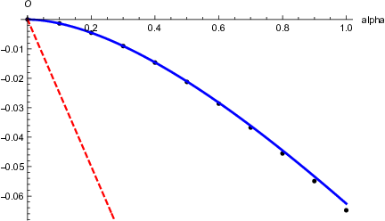
It is interesting to note that the weak coupling expansion of the octagon (3) also runs in (even) powers of . This suggests to introduce and compare the dependence of the octagon on at weak and strong coupling. Neglecting corrections suppressed by powers of , we observe (see Figure 2) that the two curves defined by (3) and (6.2) merge at intermediate values of .

Double-trace OPE channel and
As was already emphasized in Section 2.1, the leading contribution to the correlation function in this limit comes from double-trace operators. We expect that for with kept fixed, the octagon should take a finite value .
To approach this limit, we replace and in the profile function (5.2.2) and take . The leading contribution to the integral in (5.2.2) comes from whereas integration over in (5.2.2) yields a subleading contribution as . Replacing the integration variable to with , we can expand the integrand in (5.2.2) in powers of using the relation
| (112) |
This leads to the following result for the profile function for
| (113) |
where the last term accounts for the contribution from . For we have .
Substituting (113) into (58) and (5.2.1), we obtain the strong coupling expansion of the octagon
| (114) |
where the dots stand for higher-order terms in as well as terms vanishing as .
Notice that the expansion in (6.2) runs in powers of and, in order to take the limit , the series needs to be resummed. It is convenient to switch to and examine the limit with held fixed and small. Then, the relation (6.2) takes the form
| (115) |
Assuming that depends on and through , we can determine the asymptotic behavior of at small
| (116) |
In general, we can add an arbitrary constant to the right-hand side of this relation. As we show in a moment, the condition for to vanish for leaves however no room for it.
To get a closed expression for the series (115), we examine the expansion coefficients of . It turns out that they form a sequence that had already appeared in the literature, see Refs. martin2011exactly; OEIS, leading to
| (117) |
where and are modified Bessel functions. The integrand decreases exponentially fast at large and behaves as at small . Integrating by parts, we get for small
| (118) |
where
| (119) |
Imposing the condition that has to vanish for , we finally arrive at
| (120) |
We recall that this relation was obtained for and fixed. The comparison of (120) with the numerical value of at is shown in Figure 3. Integrating (6.2) with the boundary condition (120), we can obtain for arbitrary . Its expansion at large takes the form (115) with given by (116).
Notice that the resummed expression (120) vanishes for faster than the leading contribution at strong coupling. The latter is described by the first term on the right-hand side of (115). It is also interesting to note that the leading asymptotic behavior of the octagon at strong coupling is remarkably similar to that at weak coupling (see Eq. (54)) even though the two expressions are valid in different regions of the parameter space.
Null limit
In this limit, the profile function (5.2.2) can be expanded in powers of
| (121) |
where the coefficient functions are computed in Appendix D.
Using (121), we derive the strong coupling expansion of the octagon (58) and (5.2.1)
| (122) |
The leading term is
| (123) |
with the notation introduced for . The subleading terms are given by
| (124) | ||||
| (125) |
Here are the expansion coefficients of in powers of . Numerical analysis shows that
| (126) |
As before, the expansion coefficients in front of powers of in the expressions for have a uniform weight .
The expressions for contain terms enhanced by powers of . Such terms can be resummed to all orders using the property of the octagon exhibited in Eqs. (102) and (106), leading to
| (127) |
where and the profile functions , , are given by
| (128) |
The first term in (127) agrees with (6), as anticipated. The expansion (127) is well-defined for large , or equivalently for .
Comparing (122) with (4), we notice that the dependence of the null octagon on changes as we go from weak to strong coupling. In the former case, it is one-loop exact whereas in the latter case, scales as and its small expansion does not truncate.
The transition between the two regimes can be understood using the last relation in (4.2). We demonstrated in Section 3, that at weak coupling the second term in the right-hand side of this relation is exponentially small at large . At strong coupling, we replace the function in (4.2) with its leading asymptotic behavior (81) and take into account (72) to get
| (129) |
where the ellipses denote corrections suppressed by . At large , the leading contribution to the integral comes from . Changing the integration variable to and expanding the integrand at large , we find that the second term on the right-hand side of (129) behaves at small as
| (130) |
Substituting this relation into (129), we verify that the leading term cancels yielding or equivalently in agreement with (122).
7 Numerical checks
In this section, we compare numerical values of the octagon in different kinematical limits with the corresponding analytical expressions obtained in the previous section. The numerical results presented in this section were obtained in collaboration with Riccardo Guida.
To compute numerically for finite ’t Hooft coupling, we apply the relations (17) and (2.3) and truncate the size of the matrix to . In addition, we also compute a logarithmic derivative of the octagon with respect to the coupling constant, . According to (27), it is related to the potential, , which can be found from (C) by replacing the matrix with its finite-dimensional minor.
7.1 Borel–Padé improvement
At strong coupling, the octagon is given by the series expansion in , see Eqs. (102) – (104). To study its asymptotic properties, it is advantageous to consider the logarithmic derivative . It does not contain the constant term and its expansion involves only inverse powers of the coupling.
To begin with, we consider the octagon at the symmetric point . According to (6.2), it is given by a sign-alternating series in with factorially growing coefficients. Replacing values by their numerical values, we obtain
| (131) |
Following the standard procedure Bender, we can improve the strong coupling expansion (7.1) by applying the Borel transformation
| (132) |
and replacing a partial sum by its Padé approximant .
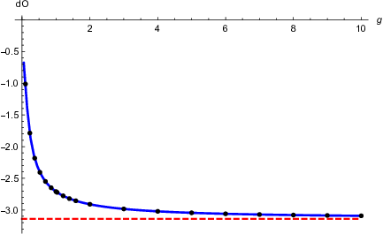
For and , the resulting expression for is shown in Figure 4. It agrees with the numerical values of the octagon up to .
We encounter similar situation in the single-trace regime, for and . Strong coupling expansion of the octagon (6.2) is Borel summable and it can be improved using the Borel–Padé method. We verified that for the resulting strong coupling expansion agrees with numerical values of up to .
7.2 Order of limits phenomenon
As mentioned in the Introduction, in the null limit, for , the octagon has different asymptotic behavior depending on the hierarchy between and . At weak coupling, for , the octagon scales as (4). At strong coupling, for , its leading behavior is given by (6) and subleading corrections are defined in Eqs. (122) and (127).
We recall that at strong coupling the relations (4) and (6) differ by the terms proportional to and they exhibit different dependence on . We will verify them in two steps. First, we put and examine the dependence of on the coupling constant at . Second, in order to check the dependence, we consider the logarithmic derivative of the ratio of octagons and examine its dependence for . We observe (see Figure 5) that the relations (4) and (127) are in agreement with numerical values at lower and higher values of , respectively. The transition between the two regimes occurs for small , or equivalently for .


8 Conclusions
In this paper, we demonstrated that the correlation function of four infinitely heavy half-BPS operators defined in (1) satisfies a system of nonlinear integro-differential equations in planar SYM. These equations are powerful enough to determine the correlation function for arbitrary values of the ’t Hooft coupling and for generic values of the cross ratios.
The starting point of our consideration was a representation of the correlation function as a determinant of a semi-infinite matrix previously derived in Refs. Kostov:2019stn; Kostov:2019auq using integrability-based hexagonalization framework Basso:2015zoa; Fleury:2016ykk; Eden:2016xvg. The matrix in question describes magnons propagating on a worldsheet of the octagon in the dual string theory and it has interesting properties. We found that it can be brought by an appropriate similarity transformation to a block-diagonal form. This allowed us to express the correlation function as a Fredholm determinant of an integral operator on a half-line with a well-known Bessel kernel modified by a cut-off Dirac-Fermi-like function. The resulting Fredholm determinant representation of the four-point correlation function has a striking similarity to two-point functions in integrable low-dimensional integrable models. Taking advantage of this fact, we applied the method of differential equations developed in Ref. Its:1990 and derived a system of nonlinear equations for the octagon.
At weak coupling, a solution to these equations yields the known expansion of the octagon over ladder integrals. At strong coupling, we developed a systematic expansion of the octagon in the inverse powers of the coupling constant and derived a representation of the corresponding coefficients as integrals of the cutoff function. We examined the resulting strong coupling expansion of the correlation function in various kinematical regions and observed a perfect agreement both with its expected asymptotic behavior dictated by the OPE as well as outcomes of numerical evaluation of the octagon. We found that, surprisingly enough, the strong coupling expansion is Borel summable. Applying the Borel-Padé method, we demonstrated that the improved strong coupling expansion correctly describes the correlation function over a wide region of the coupling constant.
There are several avenues for further studies.
Analyzing the strong coupling expansion of the octagon, we focused on perturbative corrections in and systematically discarded exponentially small nonperturbative corrections suppressed by powers of . The latter are ubiquitous to strong coupling analyses in AdS/CFT and it would be interesting to elucidate their origin. Recall that in the well-studied case of the cusp anomalous dimension, nonperturbative effects manifest themselves through Borel singularities of the strong coupling expansion in . They are associated with a formation of a mass gap in the nonlinear O(6) sigma model describing massless excitation of the string worldsheet Alday:2007mf; Basso:2009gh. Particularly, it would be important to reconcile exponentially small corrections to the octagon with the apparent fact of Borel summability of the corresponding perturbative series in .
According to AdS/CFT, the leading term in the strong coupling expansion of the octagon (58) should be given by a minimal area of a string worldsheet residing on four AdS geodesics. It would be very interesting to compute directly from string theory. Quantum fluctuations of the string generate corrections to (58) suppressed by powers of . It would be even more exciting to reproduce the relations (5.2.1) and, in particular, unravel the origin of universality of enhanced term in (58) coming from quadratic fluctuations. The method of differential equations allowed us to compute all the coefficients in (58) except the constant, independent term which appears as an integration constant in (27). One can use the relation (33) to find its dependence on the kinematical variables but the calculation turns out to be surprisingly complicated. The main reason is that the integration in (33) does not commute with strong coupling expansion of the function . Namely, all terms in expansion of this function contribute to and the strong coupling series needs to be resummed to all orders in . This question deserves a thorough investigation.
Intriguingly, the anomalous dimension describing the leading asymptotic behaviour of the null octagon (4) also controls a double-logarithmic behavior of the six-gluon MHV amplitude in a kinematical limit when three adjacent pairs of gluon momenta become collinear simultaneously Basso:2020xts. We also observed in Ref. Belitsky:2019fan that this anomalous dimension admits a complimentary description in terms of a flux-tube-like equation, whose origin remains obscure to us. These two facts hint towards the existence of a nontrivial connection between tessellation of amplitudes in terms of pentagons, on the one side, and hexagonalization of correlators, on the other.
It would be interesting to extend the formalism developed in this paper to more complicated correlation functions. The most immediate example are the octagons with nonzero internal bridges Coronado:2018ypq. They admit a Fredholm determinant representation similar to the one studied above Kostov:2019stn; Kostov:2019auq and determine the so-called asymptotic correlation functions Basso:2017khq; Coronado:2018ypq. We plan to address these questions in the future.
Acknowledgments
We would like to thank Ivan Kostov, Paul Krapivsky, Valentina Petkova, Alexander Povolotsky and Didina Serban for interesting discussions, and Till Bargheer and Pedro Vieira for careful reading of the manuscript. We are grateful to Riccardo Guida for his generous help with numerical calculations. The research of A.B. and G.K. was supported, respectively, by the U.S. National Science Foundation under the grant PHY-1713125 and by the French National Agency for Research grant ANR-17-CE31-0001-01.
Appendix A Analytical regularization
In this appendix, we discuss the strong coupling expansion of the following integral
| (133) |
where the cut-off function is given by (19). It arises as the leading term in the expansion of the moment after we replace the function with its expression (81) to the leading order in .
We perform the calculation of (133) using two different methods. The first one is based on the well-known Mellin-Barnes representation of the Bessel functions. The second one employs an analytical regularization described in Sect. 5.2.2. We show that the two methods give the same result.
To start with, recall the Mellin-Barnes transform of the product of Bessel functions in (133)
| (134) |
where the integration contour runs parallel to the imaginary axis and . Taking into account this relation, we get from (133)
| (135) |
At large , we can deform the integration contour to the right towards large positive and pick up residues at poles encountered along the way. The poles emerge from the function as well as from the integral. Similar integrals had already occurred in Eq. (97). We recall that for and, therefore, the integration over small produces poles at , or equivalently . 88 8 Here we took into account that is an even function of . Notice however that vanishes for and, therefore, the integral (135) has zero residues at all poles mentioned above except . Such pole only appears for .
In this case, we have
| (136) |
Here in the second line, the sum runs over the poles of the function and denotes the regular part of the integral. Similarly to (97) and (5.2.2), it can be found by integrating by parts times. In this manner, we obtain
| (137) |
where is the profile function defined in (5.2.2).
For , the integral in (135) is given by the sum over residues of the function
| (138) |
where is defined in (5.2.2).
Let us now reproduce the same relations using an analytical regulation. Assuming that the dominant contribution to (133) comes from , we replace the Bessel function in (133) with its asymptotic behavior at large
| (139) |
The explicit expressions for and can be read from (5.2). Replacing rapidly oscillating functions in the expression for with their mean values, we get from (133)
| (140) |
where
| (141) |
Expanding (140) in powers of , we encounter the same integral as in (5.2). We use the analytical regularization to define it according to (5.2.2). This leads to
| (142) |
It is straightforward to verify that this relation coincides with (A) for . However, for the relation (142) does not capture the leading, term in the right-hand side of (137). The missing contribution comes from the integration over the region . Indeed, restricting the integration in (133) to , we get
| (143) |
where the dots denote contributions from . Here in the second relation, we changed the integration variable to , took the limit together with .
The above analysis demonstrates that the analytical regularization captures the contribution to (133) coming from integration over and, therefore, suppressed by powers of . The remaining contribution comes from and it is controlled by the behavior of the function at small .
Appendix B Quantization condition from zeroth moment
We demonstrated in Section 5 that the relation (74), combined with the strong coupling expansion of the function (81) for , can be used to compute the octagon (58) at strong coupling.
In this appendix, we present another approach to computing the octagon. It relies on the relation (72) and makes use of the strong coupling expansion of the function (81) for . As we demonstrate below, it yields the same result for the expansion coefficients (5.2.1) and allows us to establish the relations (5.2.1) between the coefficients with odd and even indices.
We introduce and look for the solution to (69) in the form (81) with
| (144) |
where and . Substituting this ansatz into (69) and matching the coefficients in front of powers of we obtain the system of differential equations
| (145) |
We verify that, in accord with (81), the solution to the first equation is
| (146) |
Solving (B) we assume that the expansion (144) is uniform at small , i.e. , do not modify the leading small behavior and scale as for .
At small , we substitute into the second relation in (B) to find that . In a similar manner, replacing in the last relation of (B), we notice that the terms proportional to drop out resulting to
| (147) |
Equating to zero the coefficient in front of on the left-hand side we arrive at , in agreement with (5.2.1).
The same mechanism is at work for high-order functions in (144). Replacing in (144) we can obtain from (69) the system of linear equations for the coefficients . For this system turn out to be overdetermined. For the solution to exist the coefficients with odd indices have to satisfy consistency conditions. They take the form (5.2.1) and allow us to express in terms of the coefficients with even indices. To determine even coefficients , we use the relation for zeroth moment (72).
Substituting (81) and (144) into (72), we obtain the relation
| (148) |
where the notation was introduced for
| (149) |
We show below that these functions are given by series in with the coefficients depending on the expansion coefficients of the octagon (58). Equating to zero the coefficients in front of powers of on the left-hand side of (148), we can determine .
The leading function can be computed using the relations (133) and (142)
| (150) |
where is given by (5.2.2). According to (148), the contribution to should cancel against contribution from on the left-hand side of (148).
To compute we need an expression for the functions . Solving the second equation in (B) we get
| (151) |
where and are Bessel functions. Here the integration contours are chosen in such a way that the two integrals are convergent. In general, is defined up to a solution to the homogenous equation, . The value of is fixed from the requirement that at small . To fix , we require that the contribution of to should not modify asymptotic behavior of the leading function (146) at large . This leads to .
The leading, contribution to comes from the integration over small in (B). Replacing in (B) and changing the integration variable to we evaluate the leading contribution to as
| (152) |
Substituting (150) and (B) into (148) we find that the coefficient in front of vanishes provided that , in agreement with (5.2.1).
Moving on to the next order, the solution to (B) for is
| (153) |
Again, we have two integration constants and accompanying the solutions to the homogenous equation. Taking into account that and for small , it is easy to check that the integral on the second line of the last relation modifies the asymptotic behavior of at small , e.g. . Requiring such terms do not appear, we find that , independently of the values of and .
The coefficients and can be determined from relation (148). Notice that in virtue of (150) and (B), the first two terms in the left-hand side of (148) do not produce corrections and, therefore, the relation (148) leads to . Substituting (B) into (B) and going through a rather elaborate calculation, we find that term in (B) produces the contribution to that scales as . To avoid it we require that . Then, the vanishing of correction to leads to .
Appendix C Matrix representation
In this appendix, we present a solution to the differential equation (30) in terms of a semi-infinite matrix (2.3).
According to (29), the function admits a representation
| (154) |
where and the operator is defined in (22). To evaluate the second term in (154), we first determine the kernel of the integral operator
| (155) |
Replacing the kernel with its explicit expression (see the first relation in (2.4)), we get
| (156) |
where the matrix is given by (2.3). Substitution of this relation into (154) yields the following representation for the solution to (30)
| (157) |
Here the notation was introduced for
| (158) |
where and the function is defined in (19).
For the potential we find in a similar manner from (26)
| (159) |
It follows from the second relation in (C) that at weak coupling. As a consequence, the weak coupling expansion of (157) and (C) contains a finite number of terms at any order in the coupling.
At finite coupling, we can approximate the exact expressions for and by retaining a sufficiently large number of terms in (157) and (C). To this end, we replace the semi-infinite matrix in (157) and (C) by its finite-dimensional minor, . This procedure proves to be efficient in numerical analysis of the differential equation (30).
Appendix D Profile function in the null limit
Expanding the cut-off function (19) at small and large , we get
| (160) |
Substituting this relation into (5.2.2), we obtain for the profile function
| (161) |
For the leading function, the calculation gives
| (162) |
where is the Euler-Mascheroni constant. Here the first relation is exact whereas the remaining ones hold up to corrections suppressed by powers of . Note that the functions and possess weight .
For the and corrections to the profile function, we find in the same fashion
| (163) |
where . Higher order corrections to the profile function (161) are given by
| (164) |
The above relations are valid up to corrections vanishing as .
According to (161), the profile function depends on only for and . Moreover, this dependence is confined to the first two terms in the expansion.
References
- (1) A. V. Belitsky and G. P. Korchemsky, Exact null octagon, 1907.13131.
- (2) F. Coronado, Perturbative four-point functions in planar SYM from hexagonalization, JHEP 01 (2019) 056 [1811.00467].
- (3) F. Coronado, Bootstrapping the simplest correlator in planar SYM at all loops, 1811.03282.
- (4) B. Basso, S. Komatsu and P. Vieira, Structure Constants and Integrable Bootstrap in Planar N=4 SYM Theory, 1505.06745.
- (5) T. Fleury and S. Komatsu, Hexagonalization of Correlation Functions, JHEP 01 (2017) 130 [1611.05577].
- (6) B. Eden and A. Sfondrini, Tessellating cushions: four-point functions in = 4 SYM, JHEP 10 (2017) 098 [1611.05436].
- (7) Z. Bajnok and R. A. Janik, From the octagon to the SFT vertex – gluing and multiple wrapping, JHEP 06 (2017) 058 [1704.03633].
- (8) T. Bargheer, F. Coronado and P. Vieira, Octagons I: Combinatorics and Non-Planar Resummations, JHEP 08 (2019) 162 [1904.00965].
- (9) T. Bargheer, F. Coronado and P. Vieira, Octagons II: Strong Coupling, 1909.04077.
- (10) I. Kostov, V. B. Petkova and D. Serban, Determinant Formula for the Octagon Form Factor in =4 Supersymmetric Yang-Mills Theory, Phys. Rev. Lett. 122 (2019) 231601 [1903.05038].
- (11) I. Kostov, V. B. Petkova and D. Serban, The Octagon as a Determinant, JHEP 11 (2019) 178 [1905.11467].
- (12) P. J. Forrester, The spectrum edge of random matrix ensembles, Nucl. Phys. B402 (1993) 709.
- (13) C. A. Tracy and H. Widom, Level spacing distributions and the Bessel kernel, Commun. Math. Phys. 161 (1994) 289 [hep-th/9304063].
- (14) V. E. Korepin, N. M. Bogoliubov and A. G. Izergin, Quantum Inverse Scattering Method and Correlation Functions, Cambridge Monographs on Mathematical Physics. Cambridge University Press, Cambridge, 1993, 10.1017/CBO9780511628832.
- (15) A. R. Its, A. G. Izergin, V. E. Korepin and N. A. Slavnov, Differential equations for quantum correlation functions, Int. J. Mod. Phys. B4 (1990) 1003.
- (16) Y. Jiang, S. Komatsu, I. Kostov and D. Serban, Clustering and the Three-Point Function, J. Phys. A49 (2016) 454003 [1604.03575].
- (17) N. M. Bogoliubov and V. E. Korepin, Correlation length of the one-dimensional Bose gas, Nucl. Phys. B257 (1985) 766.
- (18) A. Edelman, The Distribution and Moments of the Smallest Eigenvalue of a Random Matrix of Wishart Type, Linear Algebra Appl. 159 (1991) 55.
- (19) B. Basso, G. P. Korchemsky and J. Kotanski, Cusp anomalous dimension in maximally supersymmetric Yang-Mills theory at strong coupling, Phys. Rev. Lett. 100 (2008) 091601 [0708.3933].
- (20) R. J. Martin and M. J. Kearney, An exactly solvable self-convolutive recurrence, 1103.4936.
- (21) N. J. A. Sloane, A Handbook of Integer Sequences. Academic Press, NY, https://oeis.org/A172450, 1973.
- (22) C. Bender and S. Orszag, Advanced Mathematical Methods for Scientists and Engineers. Springer Science & Business Media, 1999.
- (23) L. F. Alday and J. M. Maldacena, Comments on operators with large spin, JHEP 11 (2007) 019 [0708.0672].
- (24) B. Basso and G. P. Korchemsky, Nonperturbative scales in AdS/CFT, J. Phys. A42 (2009) 254005 [0901.4945].
- (25) B. Basso, L. J. Dixon and G. Papathanasiou, The Origin of the Six-Gluon Amplitude in Planar SYM, 2001.05460.
- (26) B. Basso, F. Coronado, S. Komatsu, H. T. Lam, P. Vieira and D.-l. Zhong, Asymptotic Four Point Functions, JHEP 07 (2019) 082 [1701.04462].