Inferring the location of reflecting surfaces exploiting loudspeaker directivity

Our model is determined by three main components: Specular reflection modeled by equivalent image sources, a loudspeaker with a non-homogeneous directivity response, and a co-located circular microphone array. Consider the set $\mathcal{S}$ containing the spatial locations of $K$ image sources of first order, i.e. $\mathcal{S}=\{\mathbf{r}_{k}\}^{K-1}_{k=0}$ for $\mathbf{r}_{k}\in\mathbb{R}^{2}$ and $K>0$. In this work we restrict ourselves to first-order images since we are considering only dominant reflections. In general the contributions of these sources dominate the early part of the room impulse response. For convenience spatial locations are expressed in polar coordinates, i.e. $\mathbf{r}=(R,\phi)$, for $R\in\mathbb{R}_{+}$ and $\phi\in\mathcal{E}=[0,2\pi)$ the angular support.

We start the analysis describing a theoretical circular array with a continuous aperture. A practical microphone array is later modeled by sampling the continuous aperture in space. Let the signal received by the continuous array be denoted by $y(t,\theta)$, with $\theta\in\mathcal{E}$. Here we assume a fixed array radius. Dependence on the radius is therefore not stated explicitly. The signal model is given by the following map:

where $L^{2}$ is Lebesgue’s space of finite energy signals. In this paper, the goal is to obtain an approximation of the inverse of the map stated in (1), i.e. to recover the image source locations from signal measurements at different angles (i.e. array positions). In later sections we show that the inverse problem can be posed as a convex optimization problem in the discrete domain. The three main components of our model are introduced next.

The system defined by $h(t,\theta)$ is described by the model’s three main components: the image source locations, the directivity information of the loudspeaker, and the influence of the microphone array geometry. It is further assumed that we can know a reasonably accurate discrete version of $h(t,\theta)$, the array geometry, and the loudspeaker’s directivity. We then aim at exploiting this information in order to find the image source locations corresponding to the dominant reflecting boundaries. Note first that in a real scenario it is necessary to have a preprocessing stage. In particular, with the right choice of excitation signals it is possible to perform an accurate deconvolution [11]. Moreover the direct path $h_{\textrm{dp}}(t,\theta)$, can in principle be estimated from anechoic measurements and be subtracted from the process.

We consider that the input to our system is a discrete version of $h(t,\theta)$ denoted by $h[n,m]$ for time steps $n=0,\dotsc,N_{h}-1$ and microphone indexes $m=0,\dotsc,M-1$. In other words, we assume we can obtain $h[n,m]$ from measurements $y(t,\theta)$. We show below how to decompose this system into its three different building blocks.

We pose the inverse problem as a linear system of equations. In this manner, we relate the vector of image locations to the linear system estimates at each of the microphones. Let us define $\mathbf{s}^{(p)}$ as a vector of size $T$, with elements $\mathbf{s}_{q}^{(p)}:=s[q,p]$, and let

where ^⊤ denotes transposition. Note $\mathbf{s}$ is of size $TMP$. The channel impulse responses to each microphone are arranged in a vector of size $N_{h}M$ as

where $\mathbf{h}^{(m)}$ has size $N_{h}$, with elements $\mathbf{h}_{n}^{(m)}:=h[n,m]$; it is the vector representation of the impulse response to microphone $m$. The forward model is now posed as

where $\boldsymbol{\Phi}$ is a matrix of size $N_{h}M\times TMP$ representing the operation in Eq. (10), and $\mathbf{n}$ is a noise term.

We conclude this section by showing how matrix $\boldsymbol{\Phi}$ is explicitly constructed. In brief we show that it has a block Toeplitz structure which, after proper zero-padding makes it amenable to implement using the FFT. We model the microphone array and the loudspeaker directivity contributions using matrices $\mathbf{A}$ and $\mathbf{D}$, respectively. Let $\mathbf{I}_{N}$ denote the identity matrix of size $N\times N$ and let us define the zero-padding matrix $\mathbf{W}_{a\times b}$ as

for some positive integers $a\geq b$. Denote by $\mathbf{F}_{M}$ the normalized DFT matrix of size $M\times M$. Then,

where $\otimes$ is the Kronecker product. We give next explicit expressions for the matrices $\mathbf{A}$ and $\mathbf{D}$.

The solution of the inverse problem consists of extracting the image source locations $\mathbf{s}$ from the channel estimates $\mathbf{h}$, i.e. an estimation of the inverse of the forward model in Eq. (13). The system of equations in Eq. (13) is in general overdetermined since $N_{h}M>TMP$. It is possible to interpret $\boldsymbol{\Phi}$ as a large dictionary of reflections where each column captures the channel response due to a single image source. In principle, the indexes in $\mathbf{s}$ corresponding to non-zero values in the solution carry image source location information. We estimate the inverse of the forward model in Eq. (13) using two different approaches.

First note that the magnitude of delay-and-sum steered-response can be computed using $\mathbf{A}^{\top}$. Also the matched filter for the loudspeaker directivity response involves multiplication with $\mathbf{D}^{\top}$. Then, the cross-correlation delay-and-sum estimate is given by

where $|\cdot|$ denotes element-wise absolute value. It is important to emphasize that this is a generalization of the methods presented in [3] and [9]. Therein, the loudspeaker is assumed omnidirectional. These approaches are known to be biased for loudspeaker impulse response mismatches and for closely spaced sources [10].

Moreover, note that the vector $\mathbf{s}$ is sparse since only a few candidate positions will be occupied by the unknown image sources. We therefore pursue a sparcity promoting solution, i.e. we write the problem as an $\ell_{1}$-regularized least squares problem,

where $\lambda>0$ is a regularization parameter.

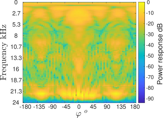
We evaluate the performance of the proposed algorithm in two different scenarios and compare it with other methods. We focus on two factors that influence performance. First, the assumption of an omnidirectional directivity pattern whereas the loudspeaker is directive. Second, the ability to resolve echoes whenever there exist more than one reflecting boundary. In particular, we consider the loudspeaker deconvolution techniques GCC-PHAT [12], cross-correlation delay-and-sum (CC-DAS) [9, 3], and $\ell_{1}$-regularized least squares (LS)[7]. In GCC-PHAT localization is performed through trilateration based on the TOA estimates of the array. An overview of these methods is provided in Table I. In high quality systems, a loudspeaker with high bandwidth that radiates homogeneously in a wide angle range is desired. The directivity function used in the experiments in depicted in Fig. 2. It is obtained from measurements in anechoic conditions. In order to assess performance in estimating location, i.e. $\hat{\mathbf{r}}$, under additive white Gaussian noise (AWGN), we have used two different metrics: the mean squared error $\text{MSE}(\hat{\mathbf{r}})=\left\|\mathbf{r}-\hat{\mathbf{r}}\right\|^{2}$, and the error rate, i.e. localization is incorrect if $||\mathbf{r}-\hat{\mathbf{r}}||^{2}>\epsilon$ for $\epsilon=0.01$, where $\mathbf{r}$ is the true source location. The MSE and the error rate can reveal the differences in performance regarding precision and accuracy respectively, i.e. a consistent bias in the estimate against correct estimates. In the experiments, we have chosen $f_{s}=48$ kHz, $R_{a}=0.035$ m, and $M=6$ microphones. The angle-dependent system impulse response $\gamma_{0}(t,\varphi)$ is measured for 12 uniform angles and truncated to $N_{v}=50$ samples. The parameters of the image source candidate locations are set to $T=78$ and $P=2$ resulting in $\mathbf{h}$ having $936$ entries. The value for $\lambda$ parameter in Eq. (23) was determined empirically.

References

- [1] F. Jacobsen and P. M. Juhl, Fundamentals of general linear acoustics. John Wiley & Sons, 2013.
- [2] T. Betlehem and T. D. Abhayapala, “Theory and design of sound field reproduction in reverberant rooms,” The Journal of the Acoustical Society of America, vol. 117, no. 4, pp. 2100–2111, 2005.
- [3] S. Tervo, J. Pätynen, and T. Lokki, “Acoustic reflection localization from room impulse responses,” ACTA Acustica united with Acustica, vol. 98, no. 3, pp. 418–440, 2012.
- [4] M. Coutino, M. B. Møller, J. K. Nielsen, and R. Heusdens, “Greedy alternative for room geometry estimation from acoustic echoes: A subspace-based method,” in IEEE International Conference on Acoustics, Speech and Signal Processing (ICASSP). IEEE, 2017, pp. 366–370.
- [5] I. Jager, R. Heusdens, and N. D. Gaubitch, “Room geometry estimation from acoustic echoes using graph-based echo labeling,” in IEEE International Conference on Acoustics, Speech and Signal Processing (ICASSP), March 2016, pp. 1–5.
- [6] F. Antonacci, J. Filos, M. R. Thomas, E. A. Habets, A. Sarti, P. A. Naylor, and S. Tubaro, “Inference of room geometry from acoustic impulse responses,” IEEE Transactions on Audio, Speech, and Language Processing, vol. 20, no. 10, pp. 2683–2695, 2012.
- [7] F. Ribeiro, D. Florencio, D. Ba, and C. Zhang, “Geometrically constrained room modeling with compact microphone arrays,” IEEE Transactions on Audio, Speech, and Language Processing, vol. 20, no. 5, pp. 1449–1460, 2011.
- [8] J. B. Allen and D. A. Berkley, “Image method for efficiently simulating small-room acoustics,” The Journal of the Acoustical Society of America, vol. 65, no. 4, pp. 943–950, 1979.
- [9] A. M. Torres, J. J. Lopez, B. Pueo, and M. Cobos, “Room acoustics analysis using circular arrays: An experimental study based on sound field plane-wave decomposition,” The Journal of the Acoustical Society of America, vol. 133, no. 4, pp. 2146–2156, 2013.
- [10] T. F. Brooks and W. M. Humphreys, “A deconvolution approach for the mapping of acoustic sources (DAMAS) determined from phased microphone arrays,” Journal of Sound and Vibration, vol. 294, no. 4-5, pp. 856–879, 2006.
- [11] G.-B. Stan, J.-J. Embrechts, and D. Archambeau, “Comparison of different impulse response measurement techniques,” Journal of the Audio Engineering Society, vol. 50, no. 4, pp. 249–262, 2002.
- [12] C. Knapp and G. Carter, “The generalized correlation method for estimation of time delay,” IEEE transactions on acoustics, speech, and signal processing, vol. 24, no. 4, pp. 320–327, 1976.