DESY 20-034
KEK Preprint 2019-57
International Large Detector
![[Uncaptioned image]](2003.01116v1/Title.png)
The ILD Concept Group
![[Uncaptioned image]](2003.01116v1/ildlogo_Zh-mumuh_sharper_blueonwhite.png)
August 11, 2026
IDR Editors
Ties Behnke1, Karsten Buesser1, Keisuke Fujii2, Frank Gaede1, Kiyotomo Kawagoe3, Jenny List1, Akiya Miyamoto2, Claude Vallée4, Henri Videau5
1
Deutsches Elektronen-Synchrotron, Hamburg and Zeuthen, Germany
2
High Energy Accelerator Research Organisation, KEK, Tsukuba, Ibaraki, Japan
3
Kyushu University, Department of Physics, Research Center for Advanced Particle Physics, Fukuoka, Japan
4
Aix Marseille Univ, CNRS/IN2P3, CPPM, Marseille, France
5
Laboratoire Leprince-Ringuet, Institut Polytechnique de Paris, Palaiseau, France
ILD authors
H. Abramowicz52, T. Agatonovic Jovin64, O. Alonso55, M.S. Amjad56, F. An21, L. Andricek16, M. Anduze35, J. Anguiano29, E. Antonov37, Y. Aoki30, F. Arteche27, D. Attié8, V. Büscher60, O. Bach12, V. Balagura35, J. Baudot25, V. Begunov17, S. Behera22, T. Behnke12, A. Bellerive7, D. Belver9, Y. Benhammou52, M. Berggren12, C. Berriaud8, G. Bertolone25, M. Besançon8, A. Besson25, J. Beyer12, O. Bezshyyko54, D.S. Bhattacharya49, P. Bhattacharya49, G. Blazey45, V. Bocharnikov12, M. Boronat19, O. Borysov12, R. Bosley3, V. Boudry35, D. Boumediene36, C. Bourgeois34, I. Bozovic Jelisavcic64, D. Breton34, E. Brianne12, J.-C. Brient35, K. Briggl58, K. Buesser12, S. Callier46, E. Calvo Alamillo9, C. Carrillo9, A. Catalán19, M. Chadeeva37, P. Chau60, M. Chera12,a, B. Chetverushkin17, M. Chrzaszcz20, G. Claus25, P. Colas8, C. Colledani25, C. Combaret26, R. Cornat38, F. Corriveau40, M. Danilov41, C. de la Taille46, Y. Deguchi33, K. Desch5, A. Dieguez55, R. Diener12, M. Dixit7, M. Dong21, A. Dorokhov25, G. Dozière25, A. Drutskoy37, F. Dulucq46, A. Dyshkant45, E. Edy35, G. Eigen2, U. Einhaus12, Z. El Bitar25, A. Elkhalii6, L. Emberger42, D. Esperante19, R. Eté12, Y. Fang21, O. Fedorchuk12, M. Firlej1, T. Fiutowski1, I. Fleck51, N. Fourches8, M.C. Fouz9, K. Francis45, K. Fujii18, K. Fujii30, E. Fullana19, T. Fusayasu48, J. Fuster19, P. Göttlicher12, K. Gadow12, F. Gaede12, A. Gallas34, S. Ganjour8, I. García19, H. García Cabrera9, G. Garillot26, E. Garutti14, F. Gastaldi35, P. Ghislain38, M. Goffe25, P. Gomis19, W. Gong21, A. Gonnin34, D. Goswami22, K. Goto33, C. Graf42, I.-M. Gregor12, G. Grenier26, R. Guillaumat35, M. Habermehl12, L. Hagge12, O. Hartbrich12,b, F. Hartjes44, H. Henschel12, D. Heuchel12, S. Hidalgo23, A. Himmi25, T. Hu21, C. Hu-Guo25, J.-C.T. Ianigro26, M. Idzik1, A. Irles34, H. Ishihara50, A. Ishikawa30, L. Jönsson39, K. Jaaskelainen25, D. Jeans30, J. Jeglot34, G. Kacarevic64, M. Kachel25, S. Kajiwara18, J. Kalinowski62, J. Kaminski5, Y. Kamiya18, R. Karl12, Y. Kato18, Y. Kato31, S.-i. Kawada12, K. Kawagoe33, S.A. Khan13, C. Kleinwort12, P. Kluit44, M. Kobayashi30, C. Koffmane16, S. Komamiya61,d, S. Korpachev37, K. Kotera50, U. Krämer12, K. Krüger12, J. Kunath35, M. Kurata30, T. Kurca26, J. Kvasnicka24,c, D. Lacour38, I. Laktineh26, W. Lange12, S.-L. Lehtinen12, T. Lesiak20, A. Levy52, I. Levy52, B. Li26, G. Li21, C. Ligtenberg44, B. List12, J. List12, L. Liu18, Y. Liu21, Z. Liu21, W. Lohmann12, M. Louzir35, S. Lu12, B. Lundberg39, J. Maalmi34, F. Magniette35, N. Majumdar49, Y. Makida30, P. Malek12, J. Marín9, J. Marshall63, S. Martens14, G. Martin-Chassard46, L. Masetti60, R. Masuda18, H. Mathez26, T. Matsuda30, K.T. McDonald47, D. Mikhaylov17, L. Mirabito26, S. Miroshin37, W. Mitaroff15, A. Miyamoto30, T. Mizuno30, U. Mjörnmark39, T. Mogi18, G. Moortgat-Pick12, F. Morel25, S. Moreno55, T. Mori18, J. Moron1, D. Moya11, S. Mukhopadhyay49, Y. Munwes58, T. Nagamine53, J. Nanni35, O. Napoly8, S. Narita28, J.J. Navarrete9, K. Negishi28, J. Ninkovic16, A. Noori Shirazi51, T. Ogawa30, T. Okamura30, T. Omori30, H. Ono43, W. Ootani18, A. Oskarsson39, L. Östermann39, Q. Ouyang21, R. Pöschl34, J.-M. Parraud38, B. Pawlik20, G. Pellegrini23, M. Perello19, A. Perez25, H. Pham25, J. Piedrafita27, T. Pierre-Emile35, A. Pingault57, O.L. Pinto12, I. Polák24, E. Popova41, P. Poulose22, A. Pradas27, V. Prahl12, T. Price3, A. Provenza12, J. Puerta Pelayo9, H. Qi21, Y. Radkhorrami12, L. Raux46, G. Raven44, M. Reinecke12, F. Richard34, R. Richter16, S. Riemann12, M.S. Robles Manzano60, C. Rogan29, J. Rolph14, E. Ros19, A. Rosmanitz60, C. Royon29, M. Ruan21, A. Ruiz-Jimeno11, T. Sanuki53, S.K. Sasikumar12, Y. Sato53, A. Saveliev17, V. Saveliev17, O. Schäfer12, C. Schmitt60, U. Schneekloth12, T. Schörner-Sadenius12, H.-C. Schultz-Coulon58, S. Schuwalow12, F. Sefkow12, N. Seguin-Moreau46, I. Sekiya33, R. Settles42, L. Shekhtman4, W. Shen58, R. Shiraz50, A. Shoji28, F. Simon42, K. Sinram12, I. Smiljanic64, M. Specht25, R. Stromhagen12, Y. Sudo12, T. Suehara33, Y. Sugimoto30, A. Sugiyama48, K. Swientek1, T. Takahashi59, T. Takeshita50, Y. Tamaya50, T. Tanabe18, T. Tauchi30, V. Telnov4, P. Terlecki1, A. Thiebault34, J. Tian18, J. Timmermans44, M. Titov8, H.L. Tran12, R. Tread50, D. Tsionou12, N. Tsuji18, B. Tuchming8, M. Tytgat57, T. Ueno53, Y. Uesugi33, S. Uozumi50, I. Valin25, C. Vallée10, H. van der Graaf44, N. van der Kolk44, B. van Doren29, A. Verdugo de Osa9, G. Vidal19, H. Videau35, I. Vila11, M.A. Villarrejo19, D. Volkov17, M. Vos19, N. Vukasinovic64, Y. Wang12, T. Watanabe32, N. Watson3, U. Werthenbach51, G.W. Wilson29, M. Wing56,c, A. Winter3, M. Winter25, T. Wojtoń20, H. Yamamoto53, S. Yamashita18, R. Yonamine53, T. Yoshioka33, B. Yu21, D. Yu21, Z. Yuan58, K. Yumino30, A.F. Zarnecki62, C. Zeitnitz6, D. Zerwas34, H. Zhao21, J. Zhao21, R. Zhao25, Y. Zhao25, H. Zhu21, V. Zutshi45
1
AGH University of Science and Technology, Faculty of Physics and Applied Computer Science, Krakow, Poland
2
University of Bergen, Institute for Physics and Technology, Bergen, Norway
3
University of Birmingham, School of Physics and Astronomy, Edgbaston, UK
4
Budker Institute of Nuclear Physics, Siberian Branch Russian Academy of Sciences and Novosibirsk State University, Novosibirsk, Russia
5
University of Bonn, Physikalisches Institut, Bonn, Germany
6
Bergische Universität Wuppertal, Fakultät 4/ Physik, Wuppertal, Germany
7
Carleton University, Ottawa, Canada
8
Irfu, CEA, Université Paris Saclay, Gif sur Yvette, France
9
CIEMAT - Centro de Investigaciones Energéticas, Medioambientales y Tecnológicas, Madrid, Spain
10
Aix Marseille Univ, CNRS/IN2P3, CPPM, Marseille, France
11
CSIC - University of Cantabria, Instituto de Física de Cantabria, Santander, Spain
12
Deutsches Elektronen-Synchrotron, Hamburg, Germany
13
Dhofar University, Salalah, Oman
14
University of Hamburg, Faculty of Mathematics, Informatics and Natural Sciences, Hamburg, Germany
15
Institute of High Energy Physics, Austrian Academy of Science, Wien, Austria
16
Halbeiterlabor der Max-Planck-Gesellschaft, München, Germany
17
Keldysh Institute of Applied Mathematics, Russian Academy of Sciences, Moscow, Russia
18
International Center for Elementary Particle Physics (ICEPP), The University of Tokyo, Tokyo, Japan
19
CSIC-University of Valencia, Instituto de Física Corpuscular, Paterna, Spain
20
H.Niewodniczanski Institute of Nuclear Physics, Polish Academy of Sciences (IFJ PAN), Kraków, Poland
21
Institute of High Energy Physics, Chinese Academy of Science, Beijing, China
22
Indian Institute of Technology Guwahati, Assam, India
23
Centro Nacional de Microelectrónica (IMB-CNM-CSIC), Barcelona, Spain
24
Institute of Physics of the Czech Academy of Sciences, Prague 8, Czech Republic
25
Institut Pluridisciplinaire Hubert Curien, Strasbourg, France
26
Institut de Physique des deux infinis de Lyon, Villeurbanne, France
27
Instituto Tecnológico de Aragòn, Zaragoza, Spain
28
Iwate University, Morioka, Japan
29
University of Kansas, Department of Physics and Astronomy, Lawrence, KS, USA
30
High Energy Accelerator Research Organisation, KEK, Tsukuba, Ibaraki, Japan
31
Kindai University, Department of Physics, Higashi Osaka, Japan
32
Kogakuin University, Shinjuku-ku, Tokyo, Japan
33
Kyushu University, Department of Physics, Research Center for Advanced Particle Physics, Fukuoka, Japan
34
Université Paris-Saclay, CNRS/IN2P3, IJCLab, Orsay, France
35
Laboratoire Leprince-Ringuet, Institut Polytechnique de Paris, Palaiseau, France
36
Laboratoire de Physique de Clermont, CNRS/IN2P3, Aubière, France
37
P.N. Lebedev Physical Institute of the Russian Academy of Sciences (LPI), Moscow, Russia
38
Laboratoire de Physique Nucléaire et de Hautes Energies (LPNHE), Sorbonne Université, Paris-Diderot Sorbonne Paris Cité, CNRS/IN2P3, Paris, France
39
Lund University, Physics Department, Lund, Sweden
40
McGill University, Department of Physics, Montreal, Quebec, Canada
41
National Research Nuclear University, Moscow, Russia
42
Max-Planck-Institut für Physik, München, Germany
43
Nippon Dental University School of Life Dentistry at Niigata, Niigata, Japan
44
Nikhef, National Institute for Subatomic Physics, Amsterdam, Netherlands
45
Northern Illinois University, Department of Physics, DeKalb, USA
46
Centre de microélectronique OMEGA, Institut Polytechnique de Paris, Palaiseau, France
47
Princeton University, Department of Physics, Princeton, NJ, USA
48
Saga University, Department of Physics, Saga, Japan
49
Saha Institute of Nuclear Physics, Kolkata, India
50
Shinshu University, Department of Physics, Matsumoto, Japan
51
Universität Siegen, Fakultät IV, Department of Physik, Siegen, Germany
52
Tel Aviv University, Raymond & Beverly Sackler School of Physics & Astronomy, Tel Aviv, Israel
53
Tohoku University, Sendai, Japan
54
Taras Shevchenko National University of Kyiv (TSNUK), Kyiv, Ukraine
55
University of Barcelona, Barcelona, Spain
56
University College London, London, UK
57
University of Ghent, Dept. of Physics and Astronomy, Gent, Belgium
58
Universität Heidelberg, Kirchhoff-Institute für Physik, Heidelberg, Germany
59
Hiroshima University, Higashi Hiroshima, Japan
60
Johannes Gutenberg-Universität Mainz, Institute of Physics, Mainz, Germany
61
The University of Tokyo, Graduate School of Science, Tokyo, Japan
62
Faculty of Physics, University of Warsaw, Warszawa, Poland
63
University of Warwick, Coventry, United Kingdom
64
VINCA Institute of Nuclear Sciences, University of Belgrade, Belgrade, Serbia
now at Aachen Institute for Advanced Study in Computational Engineering Science (AICES),
RWTH Aachen University, Aachen, Germany
also at University of Hawai at Menoa, Department of Physics and Astronomy, Honolulu, Hawaii 96822
also at Deutsches Elektronen Synchrotron, Hamburg and Zeuthen, Germany
now at Waseda Research Institute for Science and Engineering, Tokyo, Japan
Acknowledgements
We acknowledge the support by:
the Natural Sciences and Engineering Research Council (NSERC) (Canada);
DRF (Direction de la Recherche fondamentale), CEA/DRF/IRFU, Universite Paris Saclay,
and CNRS/IN2P3 (France);
Deutsche Forschungsgemeinschaft (DFG) under Germany’s Excellence Strategy – EXC 2121 Quantum Universe – 390833306,
the German Federal Ministry of Education and Research (BMBF),
the Helmholtz Association (Germany);
the Israel Science Foundation (ISF), Israel German Foundation (GIF), the I-CORE program of the Israel Planning and Budgeting Committee, Israel Academy of Sciences and Humanities (Israel);
MEXT and JSPS under Grants-in-Aid for Science Research 23000002, 15H02083, 16H02173, 16H02176, and 17H02882 (Japan);
the National Science Centre, Poland, within the OPUS project
under contract UMO-2017/25/B/ST2/00496 (2018-2021) and the HARMONIA
project under contract UMO-2015/18/M/ST2/00518 (2016-2020) (Poland);
the Russian government under Grant RFBR 20-52-12056 (Russia);
the Spanish government MINECO/AEI through the Particle Physics program and the Unidad de Excelencia Maria de Maeztu, ref. MDM-2017-0765 (Spain);
MPNTR through the national project OI171012 (Serbia);
the Science and Technology Facilities Council, UK;
the Department of Energy (DOE) and the National Science Foundation (NSF), USA;
and the European H2020 project AIDA-2020, GA no. 654168.
We would like to thank the LCC generator working group for providing the generator files used in the Monte Carlo productions for the different analyses. This work has greatly benefited from computing services provided by the ILC Virtual Organization, supported by the national resource providers of the EGI Federation and the Open Science GRID, and of those of the German National Analysis Facility (NAF).
We like to particularly acknowledge the very fruitful discussions of the document during the final stages with Katsuo Tokushuku (KEK), Lucie Linssen (CERN) and Paul Grannis (State University of New York at Stony Brook).
Chapter 1 Introduction
The ILD detector is proposed for an electron-positron collider with collision centre-of-mass energies from 90 to about 1 . It has been developed over the last 10 years by an international team of scientists with the goal to design and eventually propose a fully integrated detector, primarily for the International Linear Collider, ILC.
The fundamental ideas and concepts behind the ILD detector have been discussed in two previous documents, the letter of intent [1] and the detailed baseline document, DBD [2]. The ILD concept has been scrutinized by international groups at different occasions. After the publication of the letter of intent [1] an international expert team reviewed ILD alongside two other detector concepts, SiD [3] and the fourth detector concept [4]. SiD and ILD were both validated as potential candidate experiments at the ILC.
ILD has been designed as a multi-purpose detector. It should deliver outstanding physics performance for collision energies between 90 and 1 TeV. The detector has been optimized to perform excellently at the initial energy of 250 , while maintaining full physics capabilities at higher energies.
A central element of the design is the capability of the detector to reconstruct precisely complex hadronic final states as well as events with leptons or missing energy in the final state. To achieve these goals, precision detector elements such as vertex detectors are combined with a large volume time projection chamber for excellent tracking efficiency and with a highly granular calorimeter, in an overall design philosophy called particle flow, developed for optimal global event reconstruction.
In this document the current state of the design of the ILD detector is summarised. The technologies which are proposed for the different parts of the detector are introduced. An extensive benchmarking has been performed to demonstrate the physics performance of ILD. In order to ensure a detector adequacy for the whole ILC program, including possible future energy upgrades, benchmarking has been mostly done at a collision c.m.s energy of 500 GeV instead of the initial 250 GeV energy. Two detector configurations, a large and a smaller one, have been simulated in detail to provide guidelines towards an optimal balance between performance and cost.
A lot of the work presented in this report is based on detector R&D work which has taken place over the past decade to develop the necessary technologies. This work has been typically conducted within dedicated R&D collaborations, which are independent but maintain very close connections to ILD. All technologies selected by ILD for its subsystems have been proven experimentally to meet the performance goals, or to come very close. Developing a very powerful detector concept over a long period of time requires balancing cutting edge technologies, which might become available while the concept is being developed, with safe and sound solutions. ILD in many cases is pursuing more than one technological option, to remain flexible and to be able to adapt to new developments. The concept group wants to remain open and flexible to be prepared to select the most modern and most powerful technology once it is necessary.
The ILD concept group has currently 64 member institutes from all around the world. The group has evolved into a proto-collaboration, which is positioning itself to move forward with a proposal for a detector at the ILC or other proposed electron-positron facilities.
The document starts with a short review of the science goals of the ILC, and how the goals can be achieved today with the detector technologies at hand. After a discussion of the ILC and the environment in which the experiment will take place, the detector is described in more detail, including the status of the development of the technologies foreseen for each subdetector. The integration of the different sub-systems into an integrated detector is discussed, as is the interface between the detector and the collider. This is followed by a concise summary of the benchmarking which has been performed in order to find an optimal balance between performance and cost. To the end the costing methodology used by ILD is presented, and an updated cost estimate for the detector is presented. The report closes with a summary of the current status and of planned future actions.
Chapter 2 Science with ILC
The ultimate goal of fundamental physics is to achieve a unified understanding of nature, including matter, forces and space-time. Within the Big Bang model, the early universe before formation of hydrogen atoms is characterised by a hot dense state which was opaque to light and cannot be directly observed by optical telescopes. Its behaviour is governed by microscopic physics of fundamental particles and forces. Energy frontier collider experiments provide a unique opportunity to investigate the physics of this early universe by reproducing in a controlled manner reactions that happen in very hot dense states. Our current understanding of microscopic physics is summarised in the Standard Model (SM) of particle physics. The SM consists of matter fermions (quarks and leptons), force carrying vector bosons (gauge bosons), and a scalar boson (Higgs boson) designed specifically to give masses, where needed, to otherwise massless SM particles by breaking the electroweak symmetry through Higgs condensation in the vacuum. The 2012 discovery of the Higgs boson at the LHC has completed the SM particle spectrum.
Up to now, the SM has survived all the intense scrutiny through searches for new particles at energy frontier colliders such as LEP, HERA, Tevatron, and, most recently, the LHC, as well as through precision measurements of electroweak observables. However, while being extremely successful, the SM leaves many open questions such as: What is the nature of dark matter and dark energy? Why does matter dominate over antimatter in the universe? What is the origin of neutrino masses and mixings? And why did the Higgs field fill the entire universe and why at the electroweak scale? These questions call for physics beyond the Standard Model (BSM). The Higgs boson, through its central role at the heart of the Standard Model and its very specific scalar nature, opens new avenues to address these issues. The Higgs boson discovery hence marked the start of a new voyage towards a better understanding of the physics of the early universe.
The ILC is going to explore uncharted waters at and beyond the electroweak scale, corresponding to about one trillionth of a second after the Big Bang, in order to directly address the question: why did the Higgs field fill the entire universe and why did it do so at the electroweak scale? Precision Higgs studies are of utmost importance to answer this question. The ILC will fully exploit the Higgs boson as a new tool to discover BSM physics responsible for the mystery of the electroweak scale.
A key observable is precision measurements of Higgs couplings to various SM particles. In the SM the Higgs boson’s couplings to various SM particles are proportional to their masses. BSM physics modifies this proportionality, leaving its nature imprinted in the deviation pattern from the SM, which would allow to discriminate possible new phenomena such as existence of another dimension, a deeper stratum of matter, or a ”multi-verse”.
The ATLAS and CMS experiments at the LHC have measured the Higgs couplings to the vector bosons and the third generation matter fermions and found them consistent with the SM predictions within errors at the 10 % level [5]. The high-luminosity LHC (HL-LHC) is expected to significantly improve the measurement accuracy to a 2-4 % level [5]. These accuracies would be, however, insufficient, since deviations are typically expected at a level of 5 % or smaller due to the famous decoupling theorem [6]. To see the deviations and their pattern and to decide the future direction of particle physics, a percent level precision for various Higgs couplings is needed.
The primary goal of the ILD experiment is to measure various Higgs couplings to a % level or better, so as to make a decisive step in deciphering the physics beyond the Standard Model, and to help to decide the future direction of particle physics from their deviation pattern. ILD is also to measure properties of the and bosons and fermion pair production with unprecedented precision, while searching directly for new particles with unprecedented sensitivity, in order to further elucidate new physics that lies beyond the electroweak scale.
To achieve this goal, the ILD experiment has to reach a new level of precision in the reconstruction of final states. It aims at reconstructing every event at the level of quarks, leptons, and fundamental bosons including gauge bosons and the Higgs boson, so as to see events as if viewing a Feynman diagram. For this purpose, the ILD design has been optimized for Particle Flow Analysis (PFA), enforced by precision vertexing to tag heavy flavors and hermeticity to indirectly detect invisible particles such as neutrinos and dark matter particles.
To benefit maximally from the energy upgradability of the ILC machine, ILD has been designed to be an experiment at a collider providing electron-positron collisions at centre-of-mass energies between 90 GeV and about 1 TeV, which allows a broad and long-term physics program that will evolve depending on the results from earlier stages. New particle searches at higher energies guided by a specific deviation pattern of Higgs couplings found at 250 GeV are a typical case of such evolution. There is, however, a set of guaranteed physics of crucial importance at higher energy stages. The top quark, which is the heaviest in the SM and hence expected to be tightly coupled to the electroweak symmetry breaking sector, will enter our physics program at GeV. The 500 GeV stage allows to directly access the top Yukawa coupling through production and the triple Higgs coupling through production. The measurement precision for the top Yukawa and the triple Higgs couplings will be significantly improved at 1 TeV. An up-to-date presentation of the physics case of the ILC project can be found in [7] and in an extended version of this paper [8].
In the context of the ILD group a broad range of studies have been undertaken to understand the potential of the ILD experiment at the ILC up to 1 TeV. It is important to point out that these studies are based on fully simulated events, using a realistic detector model and advanced reconstruction software, and in many cases include estimates of major systematic effects. This is particularly important when estimating the physics reach of ILC and ILD for specific measurements. Determining, for example, the branching ratios of the Higgs boson at the percent level depends critically on the detector performance, and thus on the quality of the event simulation and reconstruction.
It should also be emphasized that, in many cases, the performance used in the physics analyses has been tested against prototype experiments. The performance numbers decisive for vertexing, tracking, and calorimetry are all based on results from test beam experiments. These test beam results include those regarding single particle resolution for neutral and charged particles, particle separation in jets, one-to-one linking power between charged tracks and calorimeter clusters, and many aspects of detailed shower analyses. The PFA performance, a crucial element that decides the ILD physics reach, has been corroborated by these test beam results, though its full demonstration has to wait for a larger scale test beam experiment that combines these major detector aspects. A very brief summary of the main results from the ILD full simulation studies is given in the next sections of this chapter.
1 Higgs Physics
One of the most important Higgs measurements at the ILC is that of the process with the recoil mass technique, which allows to measure the total production cross section () independently of the decay modes, and hence to absolutely normalise Higgs couplings. This is in contrast to measurements at the LHC, where initial state 4-momenta of colliding partons are unknown and hence the recoil mass technique cannot be applied. Figure 1 (left) shows the mass distribution of the system recoiling against the pair from a decay[9]. A clear Higgs peak sticks out from the background, independently of the decay products of the Higgs boson. This will allow to determine the Higgs boson mass to MeV with at GeV.

With the same integrated luminosity, by combining the and channels, the absolutely normalised can be measured to 2.0 % for both and beam polarisations.
The same technique can be used to search for a new scalar boson or the Higgs to dark matter invisible decays. Figure 1 (right) shows expected recoil-mass peaks of additional scalar bosons with various different masses, assuming, here for display purpose, that they have the same coupling to as the SM Higgs boson. Notice that the high momentum resolution from the ILD tracking is essential to see these sharp peaks with a width dominated by the beam energy spread instead of detector resolution. The ILD will allow to put a 95 % C.L. upper limit of 1 % or better on the cross section normalized to the SM value for such extra scalar bosons with masses below 120 GeV. The search for the invisible Higgs decays can take advantage of the higher branching ratio for hadronic decays. With the 2 ab-1 at GeV, ILD will be able to put a 95 % C.L. upper limit of 0.3 % on [10].
The measured with the recoil mass technique is used to extract the branching ratio of the Higgs boson to a pair of SM particles () from its corresponding measurement. Here the ILC’s clean environment and ILD’s excellent flavor tagging capability play a central role to separate and decays, not to mention the dominant decay. While the direct detection of the and decays is challenging at the LHC, the LHC can measure the ratios of branching ratios to high precision for decay modes with small branching ratios as long as they have clean signatures. For a Higgs decay such as which has a branching ratio of a per-mille level, its measurement at the ILC alone will be statistics-limited. The combination of the measurement of the ratio, at the LHC and that of at the ILC allows the measurement of the coupling to 1 %, which is a typical example of LHC-ILC synergy.
In order to extract an absolutely normalized Higgs coupling, , from the corresponding measured branching ratio, , the total width, , of the Higgs boson needs to be known. The total width is, however, only 4 MeV in the SM, which is too small for a direct measurement. The most recent method to overcome this difficulty and to determine the Higgs couplings is to perform a global fit in the framework of the SM Effective Field Theory (SMEFT)[11, 12]. The SMEFT framework links observables directly involving the Higgs boson to those without the Higgs boson, through the gauge symmetry. This allows to make full use of all the measurements with ILD, not only those directly involving the Higgs boson, but all the others regarding precision electroweak observables or processes without the Higgs boson such as [13]. The beam polarizations play a crucial role here to lift degeneracies between different EFT operators and to control systematic uncertainties. Figure 2 shows the projected precision of various Higgs couplings from the SMEFT fit for the 250 GeV ILC (green) and its upgrade to 500 GeV (blue), where the lighter bands assume some future improvements in ILC measurements[7].
It can be seen that, already at 250 GeV, the precisions reach the target level of 1 % for most of the major couplings, which will be significantly improved at 500 GeV.
As already mentioned above the 500 GeV stage of the ILC will provide direct access to the triple Higgs coupling, through the double Higgs-strahlung process , which has its cross section maximum at around 500 GeV. The measurement of the triple Higgs coupling is not only important for determining the shape of the Higgs potential but also crucial for testing the idea of electroweak baryogenesis. Models of this type require the electroweak phase transition to be strongly of first order, and predict an upward deviation, as large as 100 % from the SM prediction[14, 15, 16]. With 4 ab-1 at 500 GeV, the ILC can measure the triple Higgs coupling to 27 % for the SM case[17]. The precision would be improved to 15 % if the upward deviation is +100 %, being accurate enough to test such models.
2 BSM Physics
The previous section has shown how the ILD experiment will allow to achieve the ILC’s primary goal as a Higgs factory. The ILC is, however, not only a Higgs factory but also a new particle discovery machine. In general, lepton colliders are complementary to hadron colliders because of their high sensitivities to regions with small cross sections and compressed mass spectra, which are challenging at hadron colliders such as the LHC. In many cases the current best limits in such regions are still those from the LEP experiments. Though the ILC’s initial collision energy, 250 GeV, is not very much higher than the highest energy of LEP2, there are four reasons why the ILC will significantly enhance the sensitivities to these difficult regions. First, the ILC’s integrated luminosity at 250 GeV is times larger than that collected by the four LEP experiments together at the highest energies. Second, the ILD detector is much more advanced than LEP detectors thanks to the progress in detector technologies since the LEP time. Third, the ILC provides polarised beams, a very powerful tool to control signal and background processes. Finally, the ILC’s beam structure allows trigger-less data taking.
The search for weakly interacting massive particles (WIMP) pair production is one of the most important targets of new particle searches both at the LHC and the ILC. The LHC has a mass reach much higher than the ILC. Nevertheless, there will be a significant fraction of WIMP parameter space left unexplored even after the HL-LHC. The yellow area in Fig. 3 shows the remaining allowed regions after searches at the (HL-)LHC as well as current or future direct detection experiments[18].

The red solid box indicates the region the 250 GeV ILC will probe, which is already substantial. The 1 TeV upgrade will expand the ILC’s sensitivity to the red dashed box covering a large fraction of the remaining WIMP parameter space[18]. In addition to the beam polarisations, the excellent calorimetric coverage of the ILD detector, hermetic down to about 6 mrad to the beam axes, is essential to veto Bhabha background so as to achieve this high sensitivity.
A search for higgsinos is another example for which detection is challenging at the LHC because of their compressed mass spectrum. Such higgsinos are expected to be light and their mass differences typically below 20 GeV in the natural SUSY models, while the other SUSY particles may be beyond the reach of the HL-LHC. As demonstrated in [20], ILD can not only discover such higgsinos but also measure their masses and production cross sections, which can be used, together with the Higgs-related measurements described above, in a global fit to extract underlying SUSY model parameters. This in turn provides an opportunity to test high scale physics such as gaugino mass unification and various SUSY breaking scenarios. Here again, the ILD’s high sensitivity to higgsinos with small mass differences is due to the hermeticity of the ILD detector and its excellent tracking capability over a wide momentum range.
3 Top Quark Physics
As already mentioned, the top quark, being the heaviest in the SM, might hold the key to the mystery of the electroweak symmetry breaking. Its measurement starts around the threshold in the 350 GeV stage of the ILC. The threshold provides an ideal laboratory to measure a short-distance top quark mass such as . ILD can measure to 50 MeV [21, 22] and, together with the aforementioned Higgs mass measurement, test stability of the SM vacuum.
In the 500 GeV stage, our main focus of top quark physics will shift to form factor measurements for the top quark couplings to the photon and the boson. Partially composite top quarks, which often accrue from composite Higgs models, are to modify the form factors and cause significant deviations from the SM expectations with characteristic deviation pattern for couplings to and . ILD can determine these form factors separately to accuracies better than 0.3% by measuring the cross section and forward-backward asymmetry for the pair production with 4 ab-1 at 500 GeV[23]. Figure 4 compares the expected ILD precision for 500 fb-1 with various BSM models.

The form factor measurements will hence provide another handle to elucidate BSM physics responsible for the electroweak symmetry breaking, in addition to the precision Higgs measurements described above. It should be emphasized that combination of vertex charge and the Kaon ID using information from the ILD TPC plays a substantial role in the forward-backward asymmetry measurement of the production[24].
4 Benchmarking Studies
While the above physics case studies are based on the version of the ILD detector presented in the DBD [2], ILD has recently initiated a systematic benchmarking effort to study the performance of the latest updated ILD concept, and in particular to determine the correlations between science objectives and detector performance. The list of benchmark analyses is given in table 1 and their results presented in Chapter 8.
It is important to note that, although the ILC will start operation at the centre-of-mass energy of 250 GeV, the ILD detector is being designed to meet more challenging requirements at higher centre-of-mass energies, since major parts of the detector, e.g. the coil, the yoke and the main calorimeters are not expected to be replaced when upgrading the accelerator. Therefore, most of the detector benchmark analyses are performed at the centre-of-mass energy of 500 GeV, and one benchmark even at 1 TeV. The assumed integrated luminosities and beam polarisation settings follow the canonical running scenario [25].
In addition to the well-established performance aspects of the ILD detector, the potential of new features not yet incorporated in the existing detector prototypes, e.g. time-of-flight information, has also started to be evaluated.
| Measurement | Main physics question | main issue addressed |
|---|---|---|
| Higgs mass in | Precision Higgs mass determination | Flavour tag, jet energy resolution, lepton momentum resolution |
| Branching ratio | Rare decay, Higgs Yukawa coupling to muons | High-momentum resolution, identification |
| Limit on invisible | Hidden sector / Higgs portal | Jet energy resolution, or recoil mass resolution, hermeticity |
| Coupling between Z and left-handed | Contact interactions, new physics related to 3rd generation | Highly boosted topologies, reconstruction, reconstruction |
| Cross section of | Vector Bosons Scattering, test validity of SM at high energies | separation, jet energy resolution, hermeticity |
| Left-Right asymmetry in | Full dim-6 EFT interpretation of Higgs measurements | Jet energy scale calibration, lepton and photon reconstruction |
| Hadronic branching ratios for and | New physics modifying the Higgs couplings | Flavour tag, jet energy resolution |
| from and | Form factors, electroweak coupling | Flavour tag, PID, (multi-)jet final states with jet and vertex charge |
| Discovery range for low Higgsinos | Testing SUSY in an area inaccessible for the LHC | Tracks with very low , ISR photon identification, finding multiple vertices |
| Discovery range for WIMP’s in mono-photon channel | Invisible particles, Dark sector | Photon detection at all angles, tagging power in the very forward calorimeters |
| Discovery range for extra Higgs bosons in | Additional scalars with reduced couplings to the | Isolated muon finding, ISR photon identification. |
Chapter 3 The ILC Environment
In this chapter the latest status of the International Linear Collider layout and design parameters are summarized, as well as the corresponding experimental conditions for the ILD detector.
5 The International Linear Collider Project
The ILC is a high-luminosity linear electron-positron collider based on the 1.3 GHz superconducting RF accelerating technology. The ILC has been initially proposed for an energy range of 200-500 , upgradable to 1 TeV [26]. After the discovery of the Higgs Boson at 125 mass, the baseline of the ILC has been re-configured with an initial stage at 250 center-of-mass energy [8], which provides a rich harvest for a precision Standard Model and Higgs physics programme. The baseline ILC can be extended to higher energies and luminosities in well defined upgrade scenarios. The basic beam parameters for the baseline and potential upgrades are given in table 2.
Quantity Symbol Unit Initial Upgrade TDR Upgrades Centre of mass energy Luminosity Polarisation for Repetition frequency Bunches per pulse 1 Bunch population Linac bunch interval Beam current in pulse Beam pulse duration Average beam power Norm. hor. emitt. at IP Norm. vert. emitt. at IP RMS hor. beam size at IP RMS vert. beam size at IP Luminosity in top Energy loss from beamstrahlung Site AC power Site length
Recently, options for running the ILC-250 machine at the Z pole have been re-evaluated [28]. Luminosities in the order of 2.5 1033 cm-2s-1 are in reach with moderate modifications of the ILC beam parameters. Increasing this value to 5 1033 cm-2s-1 can be realised when the number of bunches per pulse is doubled, as currently suggested for the luminosity upgrade scenarios at higher energies (c.f. table 2).
The layout of the baseline 250 ILC facility is shown in figure 5. The total linear accelerator length is about 20.5 km with an experimental area hosting two detectors in push-pull configuration in the interaction region located at the center. The ILC design foresees a crossing angle of 14 mrad between the linac arms.
The Japan Association of High Energy Physicists (JAHEP) has proposed that Japan hosts the ILC as a staged project [29]. A possible site for the construction of the ILC has been idenfitied in the Kitakami mountains in the Tohoku area in the north of Honshu main island, about 400 km north of Tokyo. Figure 6 shows the location that allows for a total linac length of about 50 km, and therefore extension space for upgrade scenarios, in good geological conditions. Figure 7 shows the cross section of the ILC main linac tunnel with the cryomodules in the right section and the klystrons and RF distribution in the left section.


The specific location of the ILC site and the local conditions, e.g. in terms of street access and topography, has implications on the design, assembly and operations of ILD, as discussed in section 12.3.
6 Integration of ILD into the experimental environment
ILD is designed to operate in a push-pull arrangement with another detector, sharing one common ILC interaction region. In this scheme ILD sits on a movable platform in the underground experimental hall. This platform allows for a roll-in of ILD from the parking position into the beam and vice versa within a few hours. The detector can be fully opened and maintained in the parking position.
The current mechanical design of ILD assumes an initial assembly of the detector on the surface, similar to the construction of CMS at the LHC. A vertical shaft from the surface into the underground experimental cavern allows ILD to be lowered in five large segments, corresponding to the five yoke rings.
ILD is designed to fully cope with the ILC beam conditions (c.f. Section 16). The expected levels of beam induced backgrounds have been simulated and are seen to be at tolerable levels, e.g. for the vertex detectors. Judiciously placed shielding keeps scattered backgrounds under control. Regarding the collider, the design of the interaction region and the collimation system has been defined so as to keep the external background sources at levels below the detector requirements.
ILD is self-shielding with respect to radiation and magnetic fields to enable the operation and maintenance of equipment surrounding the detector, e.g. cryogenics. Of paramount importance is the possibility to operate and maintain the second ILC push-pull detector in the underground cavern during ILC operation (c.f. Section 12).
7 Experimental Conditions
7.1 Beam Conditions
The ILC beams have specific properties that are optimised for the physics output of the experimental programme:
- •
High instantaneous luminosity: 1.351034cm-2s-1 at 250 cms;
- •
Longitudinal polarisation for the electron (80%) and positron (30%) beams;
- •
Moderate energy losses from beamstrahlung;
- •
A pulse structure with pulse lengths of 1 ms and low repetition rates of 5-10 Hz which enables the use of power-pulsed readout schemes in the detector.
- •
A beam crossing angle of 14 mrad at the collision point.
To reach high luminosities, the ILC bunches are focused to very small cross sections in the nanometre range at the interaction point (see Table 2). The new baseline ILC-250 was optimised for maximum luminosity with an increased beam focusing compared to the TDR, resulting in a slightly increased beam energy spread for interactions. The luminosity spectrum describes the distribution of the luminosity versus the centre-of-mass energy. Figure 8(a) shows the luminosity spectrum for ILC-250, Figure 8(b) for the 500 upgrade.
The ILC beams produce three main sources of background in the detectors. Upstream of the collision region, the interaction of the electron and positron bunches with beam-line elements such as collimators produce high-energy highly penetrating muons parallel to the beam. Recent work has shown that the level of muon background can be reduced to a level tolerable for the detector [31], with a hit occupancy well below the critical limits.
In the collision region, the strongly focused beams emit beamstrahlung photons in the very forward directions which leave the detector towards the main beam dumps. Secondary electron and positron pairs stemming from photon conversions and interactions are a source of backgrounds especially for detectors close to the beampipe. Finally, the neutrons produced in the main beam dumps 300 m downstream of the interaction region can travel back into the detector. The three sources have been studied in detail and are under control (see section 16).
7.2 Machine Detector Interface
The requirements of a linear collider have technical implications for the ILD detector. All those aspects are summarised in the Machine-Detector Interface that has been specified and designed in close collaboration with the ILC machine groups and SiD [3], the other currently proposed detector for the ILC.
7.2.1 Push-Pull
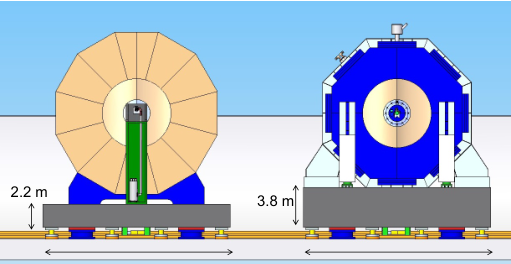
The ILC is proposed to have a common Beam Delivery System that serves one interaction point shared between two detectors, ILD and SiD, that operate in a push-pull scheme [26]. In such a scheme, one detector is taking data on the ILC beam, while the other one is parked close by and waits for its turn to move in. Figure 9 shows a conceptual design of ILD and SiD in such a push-pull configuration where both detectors are mounted on movable concrete platforms. The system is designed for short turn-around times of one day or less.
7.2.2 Accelerator Elements
The final focus magnets of the ILC are at a close focal length so that they have to be accommodated by the detectors. The closest magnet to the interaction point, the QD0 quadrupole, is an integral part of ILD, as can be seen in figures 10 and 14. The QD0 magnet packages move together with the detector in case of push-pull operations, i.e. SiD and ILD both have their own set of magnets.

In the ILC TDR, two focal lengths of the QD0 magnets were foreseen, 4.4 m for ILD and 3.5 m for SiD [26]. Later, the design of the ILC has been changed and the focal lengths were harmonised at 4.1 m [33]. For ILD, this required a re-design of the forward region, since the QD0 magnet has moved closer to the interaction point, while the detector dimension remained unchanged. A vacuum pump located close to the interaction point had to be removed to provide the required space for the change. The pump removal was expected to deteriorate the vacuum levels in the central beam pipe of ILD. However, a study of the possible impact on backgrounds from beam-gas reactions showed that the estimated levels are still negligible [34].
Chapter 4 The ILD detector concept
In this chapter, the concept of the ILD detector is presented. The basic idea has not changed since the ILD-DBD and is shortly repeated below. Recently, a re-optimisation process of the ILD configuration has been initiated in order to find an adequate balance between performance and cost of the detector. The rationale of this optimisation is presented as well as the two detector models considered for the rest of this document for performance and cost evaluation.
8 The overall ILD concept
The overall ILD concept is based on the ideas presented in the DBD [2]. The global detector layout and the performance of the subdetectors are tightly linked to the accelerator characteristics and the physics requirements, as summarised in figure 11.
The high beamstrahlung background at the collision point requires a magnetic field higher than 3 T to confine most of the low-energy electron pairs within the beam pipe, and sets a minimum of 1.5 cm for the closest distance of approach of the vertex detector inner layer from the beamline. On the other hand the bunch structure of short trains separated by long idle periods sets rather relaxed conditions on the data acquisition, with the possibility to avoid a hardware trigger system. This in addition allows to power the front-end electronics only during active bunch trains (so-called ”power-pulsing” mode), which minimises the subdetector cooling requirements and associated material budgets.
The subdetector specifications are tightly linked to the physics requirements from precision Higgs and electroweak physics. The dominant Higgs strahlung process, which at an collider provides the unique opportunity to tag Higgs production independently of Higgs decay mode, requires a very high-precision momentum measurement of isolated particles from Z decays and hence a high precision main tracker. The efficient tagging of quark and lepton flavours to disentangle Higgs couplings requires a very high precision and low-material vertex detector, which also improves on the particle momentum measurements, as well as a high calorimeter granularity to identify leptons in jets. Similarly an efficient identification of W, Z and top hadronic decays in a crowded multijet environment needs a high jet energy resolution, twice better than currently realized at LHC, as well as an efficient spatial jet separation. ILD considers that the best concept to meet these requirements altogether is particle flow, where the charged and neutral particle contents of the jets are measured with the high performance trackers and the high granularity calorimeters, respectively. Within this scheme, an efficient match between the trackers and the calorimeters requires the calorimeters to be positioned inside the coil.

9 Optimizing ILD
The baseline ILD layout of the DBD [2] had intentionally large dimensions in order to maximize the tracking performance and the particle flow capabilities of the calorimeters. The main cost drivers of the DBD detector were the electromagnetic calorimeter and the coil/yoke system, for which specific options are considered to reduce their costs (chapters 6.4 and 9). In the past years a re-optimization process of the detector global dimensions has been launched to identify an optimal point in the cost-performance space.
In a first step, a parametric study [35] of the dependence of cost and performance as function of the outer radius and length of the main tracker (the TPC in ILD) has been performed. A simple model has been constructed, based on the cost estimate published as part of the ILD DBD [2]. In this model the cost of each subdetector is scaled as a function of the size based on simple scaling laws. Sensitive detector elements like Silicon planes are scaled with the total area, while mechanical elements - for example, the absorber in a calorimeter - scale with the volume. The reference is always the DBD cost estimate. To study the effect of changing the TPC radius and length, all other dimensions outside of the TPC are tied to the TPC radius and TPC length. Clearances between detectors are kept constant, and do not scale. In this way, an overall cost scaling of the ILD detector can be computed. Comparison with the more detailed updated costing presented in chapter 9 shows that this parametric scaling if correct at the level of 20-30%.
The performance of the detector is measured by a combined performance estimator, based on a few observables mostly from Higgs physics. Essentially, these are the tracking performance (momentum resolution and impact parameter resolution), the Higgs mass precision (with and without beam-strahlung background), the inverse of the significance of b-tagging, and the minimum transverse momentum to reach the last layer of the vertex detector. All numbers are normalised to the performance of the DBD detector. For a more complete description of the method and the definitions, see [35].
Two types of iso-curves are then defined in the space opened by the TPC radius and length: Equal performance, and equal cost. In figure 12 iso-cost and iso-performance curves are shown. The three red lines correspond to costs relative to the DBD of (from top to bottom) 100%, 90% and 80%. The blue lines indicate equal-performance lines. From the plot it can be seen that the dependence of the cost on the detector radius is steeper than on the length, while the performance scales roughly the same for both. This shows that targeting a given cost reduction maintains a higher performance when reducing the radius while keeping the overall length unchanged, instead of keeping the aspect ratio r/z unchanged.
Based on this study, detector models with different sizes were defined with the following guidelines:
- •
The number of detector models is limited to two to maintain simulations and analyses at a manageable level.
- •
One of the models (”IDR-L”) has dimensions similar to those of the DBD model, in order to have a well understood reference in the studies. The only changes compared to the DBD are associated to the collider parameter evolution (e.g. the new L* optics, see chapter 3), and to better understanding of the subdetector technology constraints. This resulted in small changes to the TPC outer radius and length.
- •
The second model (”IDR-S”) has a reduced outer radius of the main tracker while keeping its length unchanged. The smaller radius has to be far enough from the IDR-L radius to provide a significant lever-arm for the comparison. The chosen value is equal to that of the new CLIC detector model CLICdp [36], half way of the even smaller radius of the SiD detector [2]. With this choice IDR-S has similar outer tracker dimensions to CLICdp for both radius and length. This offers the possibility to compare the performance of the TPC option to the all-silicon option favored by CLICdp.
- •
All other components of IDR-S are similar to IDR-L. The inner tracking and very forward detectors are identical. The calorimeter depths and cell sizes are also kept unchanged, and the number of cells is reduced only as function of the calorimeter radii. All external systems such as coil, yoke and endcaps have their radial dimensions reduced accordingly.
- •
In order to compensate for the smaller tracking lever-arm, the nominal magnetic field of IDR-S is increased from 3.5 T to 4 T.

The resulting IDR-L and IDR-S dimensions are summarised in figure 13. Both models were used for detailed simulations of physics benchmark samples. The simulation framework is described in chapter 7. The detector and physics performance of both models are compared in chapter 8 and their costing estimated in chapter 9.
Chapter 5 Detector Layout and Technologies
In the first section of this chapter the overall layout of ILD and the conceptual design of the subdetectors is summarised, with a focus on the evolution since the DBD. In the second section the results of the intense R&D performed since the DBD on the subdetector technologies is presented, and possible future steps towards a final ILD design are discussed. This chapter is intended to give a snapshot of the current state of the art and a view of the trends of future studies for the coming years.
10 Overall Structure of the Detector
The geometrical structure of the ILD detector and the individual layouts of subdetectors were described in detail in the ILD LOI [1] and the ILD DBD [2]. In this section the main characteristics with a special emphasis on recent developments and open options is given. The main design changes implemented since the DBD take into account the continuous progress in detection technologies and the new optics of the ILC interaction region (see chapter 3).
10.1 Global structure and parameters
The overall ILD detector structure is shown in figure 14: a high precision vertex detector positioned very close to the interaction point is followed by a hybrid tracking layout, realised as a combination of silicon tracking with a time projection chamber, and by a calorimeter system. The complete system is located inside a large solenoid providing a nominal magnetic field of 3.5T (IDR-L) or 4T (IDR-S). On the outside of the coil, the iron return yoke is instrumented as a muon system and as a tail catcher calorimeter.

| Barrel system | ||||||
|---|---|---|---|---|---|---|
| System | technology | comments | ||||
| [mm] | ||||||
| VTX | 16 | 60 | 125 | silicon pixel sensors | 3 double layers at | |
| (layers 1-6) | ||||||
| SIT | 153 | 303 | 644 | silicon pixel sensors | 2 double layers at | |
| (layers 1-4) | ||||||
| TPC | 329 | 1770 | 2350 | MPGD readout | 220 (163s) layers | |
| 1427s | 1×6^2 pads | |||||
| SET | 1773 | 1776 | 2300 | silicon strip sensors | 1 double layer at | |
| 1430s | 1433s | |||||
| ECAL | 1805 | 2028 | 2350 | W absorber | 30 layers | |
| 1462s | 1685s | |||||
| silicon sensor | 5×5^2 cells | SiECAL | ||||
| scintilator sensor | 5×45^2 strips | ScECAL | ||||
| HCAL | 2058 | 3345 | 2350 | Fe absorber | 48 layers | |
| 1715s | 3002s | |||||
| scintilator sensor, analogue | 3×3^2 cells | AHCAL | ||||
| RPC gas sensor, semi-digital | 1×1^2 cells | SDHCAL | ||||
| Coil | 3425 | 4175 | 3872 | 3.5 T field | int.lengths = | |
| 3082s | 3832s | 4.0 T fields | ||||
| Muon | 4450 | 7755 | 4047 | scintillator sensor | 14 layers | |
| 4107s | 7412s | 3×3^2 cells | ||||
| End cap system | |||||||
|---|---|---|---|---|---|---|---|
| System | technology | comments | |||||
| [mm] | |||||||
| FTD | 220 | 371 | 153 | silicon pixel sensors | 2 discs | ||
| 645 | 2212 | 300 | silicon strip sensors | 5 double discs | |||
| ECAL | 2411 | 2635 | 250 | 2096 | W absorber | 30 layers | incl. EcalPlug |
| 1718s | |||||||
| silicon sensor | 5×5^2 cells | SiECAL | |||||
| scintillator sensor | 5×45^2 strips | ScECAL | |||||
| HCAL | 2650 | 3937 | 350 | 3226 | Fe absorber | 48 layers | |
| 2876s | |||||||
| scintilator sensor, analogue | 3×3^2 cells | AHCAL | |||||
| RPC gas sensor, semi-digital | 1×1^2 cells | SDHCAL | |||||
| Muon | 4072 | 6712 | 350 | 7716 | scintillator sensor | 12 layers | |
| 7366s | 3×3^2 cells | ||||||
| BeamCAL | 3115 | 3315 | 18 | 140 | W absorber | 30 layers | |
| GaAs readout | |||||||
| LumiCAL | 2412 | 2541 | 84 | 194 | W absorber | 30 layers | |
| silicon sensor | |||||||
| LHCAL | 2680 | 3160 | 130 | 315 | W absorber | ||
A key feature of the detector is the amount of material crossed by the particles: particle flow requires a thin tracker to minimise interactions before the calorimeter, and a thick calorimeter to fully absorb the showers and measure neutral hadrons. Figure 15 shows the amount of radiation lengths of the tracker material and the total interaction lengths including the calorimeter system.
10.2 Subdetector layouts
The current design of subdetectors is presented including open options and critical aspects, as well as prospects for enhanced capabilities in the future. The most recent progress and status of each detection technology will be summarised in section 11.
10.2.1 Vertex detector (VTX)
The vertex detector is realised as a multi-layer pixel detector with three double-layers (Figure 16). The detector has a pure barrel geometry. To minimise the occupancy from background hits, the double-layer closest to the beam is twice shorter than the other two.

Critical parameters of the VTX optimisation are the point resolution for secondary vertex tagging, required to be better than 3, and the material thickness which should not exceed per layer to minimise multiple scattering. Three main technologies are under consideration to achieve the required goals:
- •
CMOS pixels: this well-established technology offers the advantages of high granularity with fully monolithic pixel digital electronics available from industrial processes. The most critical points of focus of current R&D [37] are the readout speed, aimed to provide single bunch tagging capacity while keeping the power consumption low enough (with or without power pulsing), and the overall material budget of the layers.
- •
DEPFET pixels: the DEPleted Field Effect Transistor (DEPFET) concept implements a first amplification stage in a FET in the high-resistivity, depleted silicon detector. Such active pixel detectors with a rolling shutter read-out can meet the stringent requirements of the ILD vertex detector [38, 39]. The technology offers the advantage of high granularity with a small layer material thickness, the digital electronics being shifted at the end of the ladders: the all-silicon ladder design [40], that is fully self-supporting and requires no external support, minimises the material in the active area to approximately 0.12% . Critical aspects of DEPFETs are the industrialisation of the fabrication process and the integration of large detector surfaces.
- •
Fine Pixel CCD (FPCCD): fine pixel CCD’s [41] offer the prospects for the highest granularities associated with low power consumption. Another advantage is the minimal material budget of the detector layer, however counter-balanced by the need of a cryostat to ensure low-temperature operation. Critical aspects under study are the readout speed and the resistance to radiation.
The CMOS and DEPFET pixels have typical sizes of 20 microns and are readout in a continuous mode during bunch trains. The readout speed determines the capability to resolve individual bunches. The FPCCD pixels accumulate hits during one bunch train before readout and reset in-between trains. Their occupancy is kept acceptable thanks to a small pixel size of order 5 microns.
10.2.2 Silicon trackers (SIT, SET, FTD)
A system of silicon trackers surrounds the VTX detector (Figure 17).
In the barrel, two layers of silicon sensors are arranged as a silicon internal tracker (SIT) to bridge the gap between the VTX and the TPC, and a one-layer silicon external tracker (SET) is foreseen in-between the TPC and the ECAL. An external tracker similar to the SET, located between the TPC flange and ECAL endcap and named ETD in the DBD, is now no longer part of the ILD design. The baseline technology for the large area trackers of the DBD was silicon strips, but the progress made since then with CMOS detectors would now allow to equip the SIT with pixels instead of strips. The design of the SET is still open including the option to implement it as the first layer of the ECAL Calorimeter. The use of sensors with a high timing resolution of O(10ps) is considered in order to provide a time of flight (TOF) functionality for particle identification.
The forward tracking detector (FTD) completes the coverage of the ILD experiment for charged particles emitted at shallow angles with respect to the beam (Figure 18). The FTD acceptance starts at 4.8 degrees, with at least one hit for tracks with polar angles below 35 degrees ( 0.82) and nearly standalone tracking for tracks below 16 degrees ( 0.96).


The first two disks are installed close to the vertex detector and are equipped with highly granular pixel detectors that provide precise 3D space points with a resolution of approximately 3-5 . The technology candidates for these disks are similar to those of the vertex detector: CMOS, DEPFET, FPCCD, SOI, and future 3D-integrated devices.
The remaining five disks extend out to the inner envelope of the TPC at 30 cm. While the requirement on the resolution of the measurement remains stringent, the cell dimension aligned with the -coordinate is less constrained. These requirements can be met with micro-strip detectors: two single-sided detectors mounted under a small stereo angle may provide the required resolution. A solution based on CMOS monolithic pixel detectors with elongated pixels is likely to be quite competitive. Also the possibility of a TOF measurement in the outermost disks merits further study.
10.2.3 Time projection chamber (TPC)
A distinct feature of ILD is a large volume time projection chamber (Figure 19 left). The TPC allows a continuous 3-dimensional tracking, dE/dx-based particle identification and minimum material. The required performance of the TPC as a standalone tracker is a momentum resolution better than GeV-1, corresponding to a single point resolution of over about 200 points, and a dE/dx resolution better than 5%. One critical issue concerns potential field distortions due to ion accumulation within the chamber. At ILC this can be mitigated by implementing an ion gating between bunch trains, using large aperture GEM foils as shown in Figure 19 right: during bunch trains, the voltage difference between the GEM sides is configured to allow drift electrons cross the GEM and reach the amplification region. Outside bunch trains, the voltage difference is reversed so that ions produced in the gas amplification region stay confined and are guided to the GEM surface where they are absorbed.


Three options are under consideration for the ionisation signal amplification and readout:
- •
GEM readout (Figure 20 left): the ionisation signal is amplified by passing through a GEM foil and is collected on pads.
- •
Micromegas readout (Figure 20 right): the ionisation signal is amplified between a mesh and the pad array where it is collected.
- •
GridPix: the ionisation signal is amplified as for the Micromegas case but collected on a fine array of silicon pixels providing individual pixel timing.
For the GEM and Micromegas options, the typical pad sizes are a few mm2 (table 3) and spatial resolution is improved by combining the track signals of several adjacent pads. For the GridPix option the pixel size of 50 microns matches the size of the mesh, providing pixel sensitivity to single ionisation electrons. The spatial resolution is improved and the dE/dx signal is measured by counting pixels or clusters.


10.2.4 Electromagnetic calorimeter (ECAL)
Electromagnetic showers are measured with a compact highly-segmented calorimeter (Figure 21) with absorber plates made of tungsten. The ECAL barrel shape is octagonal with individual stacks laid such as to avoid projective dead zones in azimuth. The baseline number of layers is 30, with options to reduce the number to 26 or even 22, keeping the amount of radiation lengths identical and increasing the thickness of the sensitive medium to maintain a similar energy resolution for single particles.

The sensitive medium consists of silicon sensors with about 5x5 mm2 pads bonded on a PCB equipped with front-end readout ASICs (Figure 22 left). In order to reduce the costs it is considered to equip part of the sensitive layers with scintillator sensors readout through SiPMs (Figure 22 right). In that case the scintillator strips would have a larger dimension of 45x5mm2 with alternate orthogonal orientation. The option to equip the first layer with high-resolution timing sensors is also under consideration to provide a time-of-flight (TOF) functionality.

10.2.5 Hadronic calorimeter (HCAL)
The hadronic calorimeter consists of 48 longitudinal samples with steel absorber plates. Two options are currently considered for the mechanical structure, differing mainly in the barrel region (Figure 23): the ”TESLA” barrel made of 2 wheels with signals extracted longitudinally in the gaps between the barrel and endcaps, and the ”VIDEAU” barrel made of 3 or 5 wheels with signals extracted at the periphery between the HCAL and coil cryostat. The TESLA wheels are assembled from iron plates screwed to each other whereas the VIDEAU wheels are self sustainable welded structures. The VIDEAU configuration presents no projective dead zone in azimuth nor at polar angle, and offers a better mechanical stiffness, at the cost of a reduced accessibility of the interfaces for data concentration and power supply.

The HCAL layers are instrumented with high granularity for an efficient separation of charged and neutral hadronic showers, necessary for particle flow, as well as for a good muon identification for flavor jet tagging. Two sensor options are under consideration (Figure 24): scintillator tiles of 3x3 cm2 with analog readout through SiPMs, and RPCs with pads of 1 cm2 readout with a semi-digital resolution of 2 bits. A timing functionality is implemented in the scintillator option and under consideration for RPCs: a resolution of O(1ns) already achieved with the scintillator option allows to tag late neutral components of the showers for particle flow, whereas a resolution of a few 10 ps, achievable with multigap RPCs, would provide TOF measurements.

10.2.6 Very forward detectors (LumiCAL, LHCAL, BeamCAL, ECAL ring)
The very forward region in the ILD detector is equipped with dedicated detectors to perform:
- •
a precise determination of the luminosity from Bhabha scattering electron pairs (LumiCAL);
- •
an extension of the hadronic calorimetric coverage in the forward region (LHCAL);
- •
calorimetric hermeticity down to 6 mrad from the beam pipe and fast monitoring of beam conditions (BeamCAL).
- •
transition between the LumiCAL and the ECAL endcap (ECAL ring).
The longitudinal configuration of the LumiCAL+LHCAL+BeamCAL system has been adapted to the new beam optics as discussed in Chapter 3 (Figure 10). The current overall layout of these detectors is shown in Figure 25.

The very forward detectors are based on similar technologies as the ILD electromagnetic calorimeter, taking into account the specific conditions of the forward region such as the harder radiation environment or the need for an improved compactness to identify electromagnetic showers in a high occupancy environment. For the detectors positioned closest to the beam pipe new sensors such as saphire are considered. The LumiCAL will be based on silicon sensors similar to the ECAL (Figure 26), with thinner instrumentation layers to minimize the lateral spread of the showers.

10.2.7 Iron yoke instrumentation
A large volume superconducting coil surrounds the calorimeters, creating an axial -field of nominally 3.5 Tesla (IDR-L) or 4 Tesla (IDR-S). An iron yoke returns the magnetic flux of the solenoid, and, at the same time, serves as a muon filter, muon detector and tail catcher calorimeter. The baseline structure of the yoke is shown in Figure 27 left for a configuration accounting for the maximum stray fields allowed in the push-pull configuration (chapter 3). Optimization of the yoke size is ongoing to minimize the overal cost driven by the amount of iron (section 6.4.2). A number of iron yoke gaps will be instrumented for muon tracking and measurement of the tails of the hadronic showers. The required muon tracking precision is of the order of 1 cm in azimuth and of a few cm longitudinally. The instrumentation is expected to consist of scintillator bars but RPCs are also considered. In the scintillator option the light will be collected by wave length shifting (WLS) fiber readout with SiPMs at both ends [42] (Figure 27 right top). The WLS fibers will be positioned either in an extruded groove at the center of the large side of the bar (Figure 27 right middle), or along the small side of the bar (Figure 27 right bottom).

11 Subdetector Technology Status
All ILD detector technologies under consideration have benefited from substantial developments since the DBD publication. Many activities are coordinated within worldwide R&D Collaborations such as LCTPC [43], CALICE [44] or FCAL [45]. Compared to the DBD studies, which were still focused on intrinsic physics response and performance, many technologies have now developed operational implementations with technological prototypes which are mature for extrapolation to a full detector. Applications have indeed already started with many spin-offs to existing experiments such as the high-luminosity LHC detector upgrades. The experience gained with these projects will be a strong asset to the final design and construction of ILD.
11.1 Vertex Detector
The vertex detector is a high-precision small device which is expected to be one of the latest subdetectors to be built and inserted within ILD. The development of optimal technologies can therefore proceed until a few years before the start of ILC. There has been much progress in this direction in the past 5 years for the three main options under consideration: CMOS, DEPFET and FPCCD sensors.
11.1.1 CMOS sensors
The use of CMOS sensors for particle physics has benefited a lot from the development in the past two decades of the MIMOSA chip series by the IPHC Institute. A first full scale particle physics detector application has been realized with the STAR vertex detector [46] (Figure 28) on the RHIC hadron collider. Since then the technology has further developed as a widespread standard for pixel detectors, including many applications to e.g. LHC upgrades or new experiments.
The general trend of performance improvements towards ILD specifications is summarized in table 5. Compared to STAR the new applications for the ALICE upgrade [47] and CBM at FAIR [48] have moved to a technology with a smaller pattern, have implemented a new data driven readout scheme, and have improved the time resolution and power consumption to values close to ILD needs. The ALICE detector also concerns a very large area of more than 10 m2, which qualifies the technology for the inner layers of a central tracker.
With these applications more attention is given to integration aspects of the technology. The chip intrinsic power consumption is now close to the ILD specification and could still be reduced by a factor 10-20 with power pulsing. To this respect a trade-off will have to be made between readout speed (related to time resolution) and power. With the expected heat production air cooling as done at STAR could be sufficient, but ILD has stronger constraints on the possible air flow due to a more forward instrumentation than STAR. This critical issue requires further studies. Low material ladder supports have been developed with the PLUME concept [49], consisting of a thin foam layer carrying pixel chips on both sides as a double layer. First PLUME ladders have been built and a second version has been successfully operated for the BELLE II beam commissioning (Figure 29 top).
| DETECTOR: | STAR-PXL | ALICE-ITS | CBM-MVD | ILD-VXD |
| (ULTIMATE) | (ALPIDE) | (MIMOSIS) | (PSIRA) | |
| 2014-16 | 2021-22 | 2021-22 | 2030 | |
| Technology (AMS): | 0.35 m | 0.18 m | 0.18 m | 0.18 m |
| Pixel size (m: | 20.7 x 20.7 | 27 x 29 | 22 x 33 | 22 x 22 or 18 x 18 |
| Readout mode: | rolling shutter | data driven | data driven | data driven |
| Time resolution (s): | 135 | 5-10 | 5 | 1-4 |
| Power (mW/cm2): | 150 | 35 | 200 | 50-100 |
| Material (/layer): | 0.39% | 0.3% | - | 0.15% |

11.1.2 DEPFET sensors
The development of DEPFET sensors in particle physics is reaching maturity. Following the demonstration of small prototypes [50, 51] and first operational ladders five years ago the technology was chosen as the baseline for the vertex detector [52] of the Belle II experiment [53]. As many requirements of Belle II are similar to those of the ILC, this can be seen as a 30% prototype of the ILC vertex detector. DEPFET ladders have been successfully used in the BELLE II beam commissioning detector (BEAST 2). The first layer of the pixel vertex detector was installed in 2018 and is now in operation in the experiment (Figure 29 bottom). Due to a low yield of the module assembly process, the second layer vertex detector is expected to be completed in 2020. While the experiment is taking data, studies towards future BELLE II upgrades based on advanced DEPFET technology are starting. The development of advanced DEPFET solutions for the ILD vertex detector is synergetic with this effort.

11.1.3 FPCCD sensors
The FPCCD technology is not yet used in full size detector applications but a first large prototype has been built [54] with a sufficient size to cover the inner layer of the ILD vertex detector. The prototype is currently undergoing detailed characterization with e.g. radioactive source signals (Figure 30). Irradiation tests of FPCCDs are also being performed since radiation hardness is a critical aspect of this technology.

11.2 Silicon Trackers
The silicon sensors surrounding the vertex detector will directly benefit from the pixel detector R&D reported above as regards their high spatial resolution components. In the past years the specific silicon R&D has focused around two lines: a generic development of high-resolution timing sensors, and the prototyping of mechanical support structures of the Forward Tracking Detector.
11.2.1 iLGADs for precise tracking and time stamping (4D-tracking)
The Low Gain Avalanche Detector (LGAD) is the baseline sensing technology of the recently proposed Minimum Ionizing Particle (MIP) end-cap timing detectors (MTD) at the ATLAS and CMS experiments. LGADs are n-on-p silicon detectors with an internal gain. To obtain this gain, an extra, highly doped, layer is added just below the p-n junction of a PIN diode. This highly doped region creates a very high electric field region. This electric field induces an avalanche multiplication of the electrons and thus create additional electron-hole pairs[55].
The current MTD sensor is designed as a multi-pad matrix detector delivering a poor position resolution, due to the relatively large pad area, around 1 mm2; and a good timing resolution, around 20-30 ps. In its current technological implementation, the signal of MIP particles hitting the inter-pad region is visible but collected with a reduced amplification which severely degrades the timing resolution. This limitation is named as the LGAD fill-factor problem. For ILD, a true 4D tracking must overcome the poor spatial resolution and fill factor limitations. A new p-in-p LGAD architecture named as inverse LGAD (iLGAD) tackles both issues [56]. Contrary to the conventional LGAD design, the iLGAD has a non-segmented multiplication layer, and it should ideally present a constant gain value over all the sensitive region of the device without gain drops between the signal collecting electrodes, see figure 31. This feature has been experimentally confirmed on a strip-like segmented iLGAD and compared against a conventional strip-like LGAD and PIN devices [57].

The tracking performances of one LGAD and one iLGAD strip detector were studied in a test beam at CERN-SPS and compared with a standard PIN strip detector. These three strip detectors were unirradiated and consisted of 45 strips with a 160 m pitch. The big advantage of the iLGAD technology was confirmed during the test beam. It was proven that while in the LGAD strip detector the signal is severely degraded in the inter-pad region, the iLGAD presents a very constant gain value over all the sensitive region of the device. These results are shown on figure 32. The charge distribution of the LGAD measured during the beam tests presents two peaks: one around 24 ke, corresponding to the MIP particles that cross the interstrip region where the generated signal is not amplified (same charge measure in the PIN strip); and one around 77 ke, corresponding to the particles that cross the region where the signal is amplified. On the other hand, the same plot produced for the iLGAD detector presents only one peak in the charge distribution around 75 ke. In this case, the signals produced for all MIP particles that cross the sensitive region of the device are amplified, resulting in a much better and uniform response along the sensitive region. The tracking and timing performances were also quantified during the test beam: the position precision reaches a few tens of microns and the timing resolution stands between 20 and 40 picoseconds depending on the amplification step features.


11.2.2 Thermo-mechanical studies of the FTD support structure
The combination of the requirements of minimal material and a mechanical stability to the level of several represents quite a challenge. A realistic, full-scale mechanical prototype of the disks has been developed to characterize their thermo-mechanical performance in conditions that resemble those of the experiment (Figure 33). This mock-up is based on a carbon-fibre support disk and 50 thick silicon petals.
The carbon-fibre disk consists of a 1 mm thick rohacell core covered on both sides by three-layer carbon-fibre skins. The resulting structure adds less than 0.04 % of a radiation length () to the material budget, when averaged over the area of the disk. The mounting points for the Silicon sensors are formed by precisely machined PEEK inserts that are glued into the carbon-fibre structure. The gluing procedure controls the relative position of the mounting points to better than 50 with a custom jig.
The Silicon petals were produced using the Silicon-on-Oxide process that is at the heart of the all-silicon-ladder concept [40]. The 50 thick sensor area is supported by a 500 thick rim.
The contribution to the material budget of the sensors and support disks is summarized in Table 6. The Silicon sensors clearly dominate the total contribution.
| Component | material (% ) |
|---|---|
| Silicon petals (active area) | 0.0500 |
| Carbon fibre (incl. cyano-ester resin) | 0.0380 |
| Honeycomb core (Aramide) | 0.0006 |
| PEEK inserts | 0.0019 |
| PEEK screws | 0.0014 |
| glue | 0.0006 |
| total | 0.093 |
The thermo-mechanical performance of the loaded disk has been tested extensively. The support disk is found to have a planarity of 200 (RMS). Despite the minimal material it is very stiff, with an eigenfrequency greater than 1 kHz. The silicon petals are mounted kinematically, such that they are free to expand in response to a thermal load, while distortions of the sensors out of the nominal plane remain very tightly constrained. The torque applied to the screws must be carefully chosen: a torque of 3 mNm is found to be optimal. With this choice, the first eigenfrequency of a free petal (167 Hz) is nearly doubled (to 270 Hz) when the sensor is clamped to the disk.
The impact of air cooling on the mechanical stability is studied with a local, laminar air flow. The power consumption pattern mimics that of a DEPFET active pixel detector, assuming that the application of power pulsing reduces the average power consumption by a factor 20. In these conditions, a gentle, laminar flow of 1 is found to be sufficient to keep the temperature gradient over the sensor to within 10∘C, Vibrations due to air flow have an amplitude of less than 1 for laminar air flow with a velocity up to 4 .
These results indicate that an aggressive design based on a thin carbon-fibre support disk and ultra-thin self-supporting Silicon petals can meet the stringent requirements on mechanical stability of the ILD experiment.

11.3 Time Projection Chamber
The ILD TPC R&D is being conducted mainly within the LCTPC Collaboration [43]. The history of these developments is described in the R&D liaison report of the Linear Collider Collaboration [58] which contains many references (pp 36-60).
The workhorse for validation of detector prototypes and operational conditions is the TPC test set-up installed permanently in the DESY test beam [59] (Figure 34). The TPC is situated in a superconducting magnet providing a magnetic field of 1 Tesla, and the beam line is equipped with precise incident and outgoing particle beam telescopes allowing to quantify the TPC reconstruction precision as function of the particle parameters. The beam test set up is currently being upgraded with the high precision LYCORIS silicon telescope [60], and a new TPC field cage with reduced field distortion is being assembled.

Significant progress has been seen in the manufacturing process of detection modules for each of the readout options. A new Micromegas layout with resistive anodes has been shown to exhibit reduced boundary distortions [61]. The flatness of the GEM modules has been improved significantly, increasing the gain uniformity by a factor 2 [62]. Operational GridPix ”QUAD” modules have been built based on the TimePix3 pixel chip [63]. Recent prototypes of the three types of detection modules are shown in Figure 35.

The performance of the three technologies has been measured in beam tests. Figure 36 shows the measured point resolution in 1 T magnetic field for drift distances from 0 to 0.6 m. This can be safely extrapolated to m in a field of 3.5 T at a drift length of 2.3 m: the higher magnetic field reduces the transverse diffusion constant in the selected gas from 91 to 30 , which compensates for the longer drift length compared to the prototype set-up. The dE/dx resolution determined by the truncated mean method has been measured to be and , respectively, for Micromegas, GEM and GridPix technologies. It improves to for GridPix using a cluster counting method. In conclusion the target requirement of a spatial resolution of m in the transverse plane, and a dE/dx resolution better than 5% have been reached in all options.


Two-track separation has also been investigated. A steel target was introduced near the TPC wall to produce multi-track events suitable for this study. From these events a 2-hit separation distance of 4 to 6 mm was measured depending on the drift distance. An algorithm based on fitting the double-hit charge deposition with expected pad response function width allowed this separation distance to be reduced to 2 mm, with 1.3 mm pads (Figure 37).

A challenging aspect of the TPC operation is the cooling of the readout end-caps, which must be realised with minimal dead material. For this a double phase cooling system with thin low-material fluid pipes has been developed and is shown to perform adequately in test-beam experiments.
Also critical for ultimate performance is the mitigation of the drift field distortions which may develop from the accumulation of ions migrating from the amplification region into the drift volume. For this an ion gating scheme based on a large aperture GEM foil (Figure 38 left) has been implemented and beam tested [64]. To prevent the positive ions created by the avalanches in the amplification device from flowing back to the drift space, a counter-field is created by applying a polarisation of -20 V between the faces of the gating GEM foil in between beam train crossings. During train crossings the voltage difference is reversed to +3 V, opening the way to the incoming electrons to be multiplied.
Results from test bench measurements show that a good transparency for drift electron signals can be maintained while reducing the accumulation of ions in the drift volume by one order of magnitude [65] (Figure 38 right).


In conclusion all basic aspects of the TPC operation have shown to meet the requirements for an experiment at the ILC.
11.4 Electromagnetic Calorimeter
The technological status of both the silicon based and the scintillator based option considered for the highly granular multi-layer sampling electromagnetic calorimeter is described in this secion.
11.4.1 Silicon option (SiECAL)
In the past five years the developments of the silicon option of the electromagnetic calorimeter has mostly focused on the design and construction of technological prototypes of the detector, and on performing beam tests.
So far square wafers with thicknesses between and processed from 6” silicon ingots have been used. An increased thickness of , already available from 6” ingots, would be conducive in case wafers from 8” ingots can be reliably produced. It would allow to reduce the number of ECAL layers to 26, without significant degradation of the energy resolution compared to the current baseline design of 30 layers (section 10.2). For the final detector, the ongoing technological developments allow to foresee to use diode matrices with a standard thickness of produced from 20 cm wafers, but the final choice of the ingot size will depend on the silicon producers chosen at the time of building the calorimeter.
Fully integrated layouts of the silicon active sensor units (ASU) have been designed with the required dimension of comprising 1024 channels. One ASU hosts 16 SKIROC ASICs [66, 67] to process 64 channels each. The top part of Figure 39 shows two recent versions of the ASU, both assembled with standard ball grid array (BGA) packaging of the ASICs. The most recent version (#13) features a separation between the power supply of the preamplifier and other power lines of the SKIROC ASIC. Big capacitances are integrated into the board design to avoid large current peaks during power pulsing. This as well as earlier versions of the ASU have been operated in power pulsed mode since 2013. The bottom part of Figure 39 shows the mechanical housing that can hold up to ten ASUs used in beam tests at CERN and DESY since 2012 [68, 69].


The response of the SiECAL technological prototype to particles is as expected [70]. The signal-over-noise ratio relevant for the internal ASIC trigger has been evaluated to be about 12.8 for a wafer thickness of . This value allows for setting the trigger threshold below the single MIP level with high efficiency. The signal-over-noise at the level of charge measurement for triggered channels is 20.4 (Figure 40 left), or better, depending on the wafer thickness. Therefore a threshold cut in the ASIC at 0.5 MIP can be applied without noise problems and with good efficiency. Response to high energy electrons has been measured at CERN in 2018 in a combined test with the SDHCAL (next section) as shown in Figure 40 right.


A long detector slab featuring a chain of eight ASUs has been built (Figure 41) and tested with MIPs [71]. A 10% signal drop has been observed along the full length of the slab and could be attributed to power voltage drops and clock reflections. An improved long slab is under construction to correct these effects and validate the system.

A new slab interface board for the digital readout of the ASUs, located at the end of the slabs, has been developed to meet the ILD integration constraints (Figure 42 left). The board integrates the digital readout of the SiECAL layers and hosts the regulators for the power supply of the ASUs, With a lateral size of about , this board already meets the tight space requirements of ILD. The board has been successfully used in a beam test in summer 2019 at DESY [72]. The slab interface boards are connected via a flat control and readout kapton cable to a concentrator unit as illustrated in the right part of Figure 42. The distinguished feature of this solution is that the kapton cable can be guided along the sides of an alveolar structure hence avoiding bulky cabling.
An ultra-thin ASU with an overall thickness of 1.2 mm has also been developed. In this version the ASICs are mounted in recessed cavities of the PCB in a so-called chip on board (COB) packaging (Figure 43). First tests of the COB ASUs have been successfully performed at the 2019 beam test at DESY [72]. Clean MIP spectra have been recorded and the noise level is competitive with that of the BGA based ASUs built up to now. This is remarkable since the design of the board leaves relatively little room for decoupling capacitors. The flatness of this card meets the specifications, but the yield has to be studied with industry. Further tests will be performed and industrial aspects will have to be investigated further.
The R&D in the coming years will further emphasise system and integration aspects based on the current achievements. The planned R&D includes a new version of the ASIC with full zero suppressed readout, which implies an utmost stable pedestal level.


The silicon technology developed for ILD has been adopted as the baseline for the electromagnetic end-cap section of the CMS High Granularity Calorimeter (HGCAL) upgrade [73]. The HGCAL layout is based on hexagonal readout modules with a technology similar to the ILD one. It incorporates a new version of the SKIROC ASIC with a sub-ns timing functionality which may also be of interest for the ILD detector. A HGCAL prototype of 27 layers has been successfully tested by CMS in a combined beam test at CERN with the AHCAL ILD prototype (next section). The full HGCAL represents a 10% prototype of the ILD SiECAL w.r.t. the silicon diodes surface. Despite many differences between the ILD and CMS designs, the HGCAL construction will be a strong asset to validate the large scale assembly and fabrication processes for ILD.
11.4.2 Scintillator option (ScECAL)
Similar to the silicon option, the scintillator option of the electromagnetic calorimeter, after the validation of the concept using the physics prototype, has focused its R&D towards a technological prototype with fully integrated detection layers. The design of the detection layer is based on an integrated readout board, called ECAL base unit (EBU), of with four SPIROC ASICs developed by OMEGA group[74] on which 144 scintillator strips ( each) coupled to SiPMs are mounted.
Notable progress has recently been made on the SiPMs for the ScECAL. MPPCs with a smaller pixel pitch of 10 or have been developed, which can provide a large dynamic range as required for the ScECAL[75]. Further improvements have been made for the most recent small-pixel MPPCs, including reduced optical cross-talk by a trench structure between pixels, lower dark noise and higher photon detection efficiency. These have been confirmed by the prototype tests.
In the previous prototype studies, the SiPM was attached to the side edge of the strip. New designs of the SiPM readout at the bottom side of the strip are being developed for more uniform response and a better compatibility with future large-scale production. Especially a recently proposed design based on a strip with a dimple directly coupled to a surface-mounted SiPM on the PCB, similarly to the SiPM-on-tile technology of the AHCAL (see next section), shows a promising performance with a reasonably high light yield and a uniform response over the strip length (Figure 44). Another design of the SiPM readout is also being studied, where the strip is readout by two SiPMs set in coincidence, which reduces random noise and hence improves the signal to noise ratio. For this design a twice longer strip () is expected to be used in order not to increase the number of SiPMs.
Low cost and high light yield plastic scintillator materials are also being developed for the ScECAL. The development focuses on the polystyrene-based scintillator produced by the injection moulding method, which is suitable for large-scale production. A reasonably high light yield of 65–70% of that of the commercial PVT-based scintillator, has been achieved by optimizing the production parameters.
Detection layer prototypes have been developed with the small pixel MPPCs ( pixel pitch) as shown in Figure 45 left. A prototype layer was tested in positron beams of 50–800 MeV at the ELPH facility of the Tohoku University. Figure 45 right shows the typical charge distribution obtained for the positron beam, with the MIP peak well separated from the pedestal.

A fully integrated technological prototype with 30 alternating absorber and detection layers is planned to be constructed as a joint effort with the ScECAL R&D for CEPC to demonstrate the performance of the ScECAL technology and its scalability to the full-size detector.
11.5 Hadronic Calorimeter
The technological status of both options considered for the highly granular multi-layer sampling hadronic calorimeter is summarised below.
11.5.1 Scintillator option (AHCAL)
A CALICE AHCAL physics prototype was built and operated in 2006-2011, allowing to demonstrate the particle flow [76] and energy resolution performance [77] of the scintillator SiPM (”SiPM-on-Tile”) technology for the DBD. In subsequently published papers [78, 79, 80, 81, 82, 83, 84] the adequate modelling of instrumental effects and shower evolution has been further established, and the hadronic energy resolution and linearity of a combined system with a scintillator tungsten ECAL in front was shown [85] to be as good as that of the AHCAL alone, see Figure 46. The software used to model the detector effects such as photo-electron statistics in the SiPM has been validated by the test beam data and is also used in ILD, after adjusting for a small difference in sampling fraction only [86].
With the establishment of the principal viability of the AHCAL technology, the focus has shifted from the study of the physical performance characteristics of such a detector to the demonstration of the feasibility of the concept while satisfying the spatial constraints and scalability requirements of collider experiments such as ILD. For this purpose a new AHCAL technological prototype has been built. It is based on a scintillator tile design well-suited for mass production and automatic assembly, originally proposed in [87] and subsequently varied and optimised in further studies [88, 89].
The new AHCAL technological prototype [90] consists of a non-magnetic stainless steel absorber structure with 38 active layers and has 21888 channels. The structure has been produced from standard rolled plates, which had undergone a cost-effective roller-levelling procedure, ensuring a flatness of mm, demonstrated over an area of 22 m2. The plates were assembled using screws as foreseen for the full ILD structure in the TESLA mechanical layout. The basic unit of the active elements is the HCAL Base Unit HBU [91], with a size of 36 36 cm2, holding 144 SiPMs controlled by four SPIROC2E ASICs [74]. A key element of the electronics is the capability for power-pulsed operation. In addition to dual-gain energy measurement, the electronics also provides a cell-by-cell auto trigger and time stamping at the few ns level in test beam operations. In operating conditions with shorter data-taking windows closer to the bunch train structure of linear colliders, sub-ns time resolution is achieved.
The prototype uses Hamamatsu MPPC S13360-1325PE photon sensors and injection-moulded polystyrene scintillator tiles with a central dimple [89] for optimal light collection, as shown in Figure 47.


Spot-samples of all SiPM lots, and each individual ASIC, had undergone semi-automatic testing procedures before soldering the HBUs [92]. The gain of the SiPMs was found to be uniform within 2.4% when operated at a common over-voltage. Without any further surface treatment, the scintillator tiles are wrapped in laser-cut reflective foil by a robotic procedure and mounted on the HBUs using a pick-and-place machine, after glue dispensing with a screen printer. The HBUs have been integrated into cassettes with interfaces for DAQ [93], LED pulsing and power distribution. The latter provides active compensation of temperature variations by automatic adjustments of the common bias voltage of the photon sensors in each layer. This was routinely used in test beam operation and stabilises the gain within . Data concentration, power distribution and cooling service systems of the prototype are also scalable to the full ILD detector.
The AHCAL technological prototype was installed in the test beam for data taking at the CERN SPS, see Figure 47. During two periods in May and in June 2018, several events with muon tracks, as well as electron and pion showers in the energy ranges 10 – 100 GeV and 10 – 200 GeV, respectively, have been recorded. Figure 48 left, from the quasi-instantaneous data quality monitoring, shows the distribution of the number of hits vs. the hit-energy weighted centre-of-gravity (cog) along the beam axis z for an electron run with a beam momentum of 100 GeV/c and admixtures of muons and hadrons. The different particle types populate different regions of the plot.

While electron showers are characterised by a relatively narrow distribution of number of hits and a cog near the front face of the detector, hadrons exhibit a wider distribution of the cog, and a larger number of hits, decreasing as the cog moves towards the rear of the detector, and leakage increases. Muons appear as a narrow band with hits and a cog on z at about half the depth of the detector.
The rich data sample collected in the two test beam periods in 2018 is being used for shower separation studies based on 5-dimensional reconstruction algorithms exploiting the high spatial, energy and time resolution of the prototype. While this is in progress, it can already be noted that in several aspects the performance exceeds that of the physics prototype: the noise is a factor 100 lower, the dynamic range of the SiPMs is 3 times larger, and 99.96% of the total 21888 channels are working.
The HBUs of the new prototype have also been used to build a large layer with two slabs of 6 HBUs each, corresponding to the full 2m length of an ILD barrel sector in the TESLA layout, see Figure 48 right. The signal quality was unaffected, and the rise time of the power pulsing was within specifications.
The AHCAL developments have also inspired the design of the scintillator section of the CMS end-cap calorimeter upgrade for the high luminosity phase of the LHC [73], and the new prototype has been used together with silicon-instrumented sections in front in a common beam test, further illustrating the maturity of the technology. The new CMS endcap calorimeter will establish the SiPM-on-Tile technology in a collider environment at an intermediate scale between the AHCAL prototype and the full ILD detector.
11.5.2 RPC option (SDHCAL)
The SDHCAL technological prototype built in 2011 has been regularly tested in beams in the past years with various configurations, including a combined test with the SiECAL prototype in 2018 (section 5.2.4.1). The SDHCAL prototype consists of 48 single-gap RPC layers of 1 m2 (Figure 49 left). Each detection gap is instrumented with 6 Active Sensitive Units (ASU) made of a 50 x 33 cm2 PCB with 24 ”HARDROC” ASICs from OMEGA [94]. The RPC pad size is 1 cm2 and the pad signals can be read out either in digital (1 bit and 1 threshold) or semi-digital (2 bits and 3 thresholds) modes (Figure 49 right).

The numerous data sets collected at CERN with high-energy hadron beams have been used to validate the performance of the technology. Special reconstruction methods adapted to the high granularity semi-digital structure of the calorimeter have been developed [95] to relate the energy estimation to the hit number and density. The current state of the performance is summarized in Figure 50. A good linearity is observed and the multi-threshold mode is found to mitigate saturation and improve the resolution at high energy. The description of the measured resolution by the simulation is however found to be sensitive to the description of the core of the hadronic showers, with a tendency for the Monte-Carlo to underestimate the performance due to harder cores in the showers [96]. This point will require further tuning of the simulation.

In recent years the SDHCAL teams have focused on adapting the technology to the full-size ILD requirements, in order to cover detection surfaces of up to 1 x 3 m2 required by the ILD Hadronic Calorimeter in its ”Videau” configuration (section 5.1.2). An improved RPC gas circulation system with better uniformity has been designed and validated with the construction of two large RPC’s. Larger ASUs of 100 x 33 have been designed with a new version of the HARDROC ASIC including zero-suppression (Figure 51 left), and their interconnection improved to allow chaining of up to 9 ASUs. Efforts have also been invested in the manufacturing process of self-sustained hadron calorimeter structures with high precision mechanical tolerance as required by the RPC insertion. A method of ”roller levelling” has been used to machine steel absorber plates with a high flatness. A high precision electro-welding has been used to build a first large size prototype of 4 calorimeter layers (Figure 51 right) which has proven that gap size variations well below 1 mm can be reached on such large structures.
For the longer term the option of multi-gap RPC’s with a high timing resolution of 20 ps is prototyped based on the ”PETIROC” ASIC [97].

11.6 Very Forward Detectors
In the past years the development of the ILD forward detectors has mostly been pursued by the FCAL R&D Collaboration [45]. Progress concerns mainly the LumiCAL calorimeter and, more recently, the BeamCAL sensors.
Based on a specific ASIC developed after the DBD, calorimeter silicon sensitive layers have been built to assemble a first LumiCAL 4-layer tungsten calorimeter prototype and, two years later, a more compact 8-layer calorimeter prototype (Figure 52 left). The two prototypes were tested with beam in 2014 and 2016, respectively. The test data [98] confirm the expected significant improvement of the transverse compactness of the electromagnetic showers in the compact prototype compared to the earlier one (Figure 52 right).
A new ASIC ”FLAME” [99] based on 130 nm CMOS technology is currently under final validation. FLAME features the low power, in-situ digitisation and fast readout required by the final detector. A new 20- layer SiW calorimeter prototype based on FLAME, with specifications and configuration close to the final LumiCAL detector, is under construction and planned to be tested with beam.

The LHCAL and BeamCAL calorimeters can be based on similar technologies as the LumiCAL, with radiation hardness requirements increasing as function of the sensor proximity to the beam. For the BeamCAL, new sensors such as sapphire are being considered. Irradiation campaigns are under way to characterize them (Figure 53) and provide input for the final choice.

11.7 Iron Yoke Instrumentation
Dedicated studies have been conducted at FNAL in the past years to optimize the layout of scintillator bars adapted to muon detection. Prototypes have been built and tested with muon beams [42]. They are all based on long scintillator bars with signal collected by WLS fibers and readout by SiPMs at both extremities. The transverse resolution of 1cm required for the muon momentum measurement is defined by the bar widths of a few cm. The longitudinal position is measured from the time difference of the signals at both extremities and depends on the WLS configuration. The two options under consideration described in section 5.1.2 (Figure 27) have been tested: longitudinal resolutions of 5 to 10 cm are measured and found roughly independent of the longitudinal position of the muon within the bar (Figure 54).
More studies are ongoing to develop low cost SiPMs also adapted to the measurement of the tails of high energy jets (tail catcher function).
The RPC option for the iron yoke instrumentation was not specifically studied but would directly benefit from the RPC developments of the SDHCAL hadronic calorimeter option (section 11.5.2).

Chapter 6 ILD Global Integration
This chapter is devoted to the diverse matters of global interest for the ILD integration, assembly and operation. These include the integration of the detector and its services within the experimental hall, the integration of subdetectors as a coherent detector, the mechanical behaviour of its components and mitigation of seismic movements, the design of the main magnet with its coil and iron yoke, mitigation of beam-related background, calibration strategies and data acquisition. All these topics still require a large amount of studies to finalise the ILD engineering design in its operational environment. There was however significant progress over the past years and the current status is summarised in the following sections.
12 External ILD integration
The proposed site for the ILC is located in the Kitakami mountains in the north of the Japanese main island Honshu. Dedicated studies are under way to adapt the generic ILC design, as described in the Technical Design Report, to the realities in this environment. For ILD, the arrangements of the surface and underground installations around the interaction point (IP) are of natural importance. The current conceptual design of the civil facilities and the plans for the detector related infrastructure and services have been coordinated between the relevant detector and ILC machine groups as well as with local experts.
12.1 Site-related Infrastructure
ILD is foreseen to be assembled on the surface, similar to CMS at LHC. Figure 55 shows a rendering of the surface installations above the ILC interaction point. At the heart is the detector assembly building that is located directly over the central shaft that gives access to the underground collider hall. A large gantry crane above the shaft allows for the lowering of the pre-instrumented detector parts into the underground area. A preparation building is foreseen where sub-detector elements can be assembled and tested. A research building and a computing building provide the infrastructure for the operation of the detectors at the IP Campus.

The underground experimental hall is about 100 m below the surface and hosts two experiments, ILD and SiD, in a ”push-pull” arrangement where both detectors share the same interaction region (Figure 56). The detectors are installed on movable platforms and can be rolled into or out of the beam line within a few hours. They can be opened and maintained in their parking positions. Access to the underground hall is provided by two vertical shafts and an access tunnel that allows for vehicles to drive directly into the underground area (Figure 57).


12.2 Detector Utilities and Cavern Ancillary Services
In order to operate the ILD detector in the underground detector cavern, electricity, cooling water and other services have to be supplied from surface facilities. Though conceptual designs existed at the time of the DBD, more detailed knowledge about the requirements from the detector exists by now and should lead to an optimisation of the facilities layout and locations.
12.2.1 Service Locations
There are several possible locations for detector services: on the detector platform, on service galleries on the wall of the detector hall, in dedicated utility/service caverns (shown as ”Utility Hall” / ”UT Hall” in Figures 56, 57), and on surface. A possible configuration is shown in Figure 58. It is assumed that large or noisy apparatus such as transformers (6.6 kV400/200/100 V), heat exchangers and pumps for cooling water, sub-detector cooling plants, etc. should be located in the utility/service cavern. Cryogenic plant for the QF1 magnet is also supposed to be located in the utility/service cavern.
The utility/service cavern should be relatively close to the detector, but well isolated from the detector hall regarding the noise, vibration, and radiation. Design of the facilities including caverns (CFS) for detector utilities/services has to be made based on requirements from the detector side. In order to clarify the requirements, a rough estimation on the ILD needs in electricity, cooling water, and space has been made (c.f. section 12.2.2).
The Design of the utility/service cavern is not fixed yet. In the baseline design (TDR-modified), the utility/service cavern had a dead-end as shown in Figure 57. In addition, this cavern was supposed to be used for both detectors and accelerators, and did not have enough space for the estimated ILD needs. ILD proposes another design as shown in Figure 59. In this design, there are two utility/service caverns, one for the accelerator and ILD, and another one for SiD. The size of the accelerator/ILD utility cavern of 25m x 25m with five floors would be large enough for accelerator and ILD, and that of 25m x 18m with three floors would be large enough for SiD. Figure 58 is drawn assuming this utility/service cavern design.


12.2.2 Power Consumption and Cooling Requirements
The requirements for power and cooling at ILD have been studied in a bottom-up approach where the current information from all detector components has been collected and cross-checked.
A tentative estimation of the power consumption in the detector hall and surface facilities for ILD is listed in Table 7. The total power consumption in the underground caverns is about 1 MW, dominated by the ILD solenoid and the machine components associated to the detector.
The cooling water which is necessary for extracting the power consumption is shown in Table 8. The sharing of the underground power is visualized in Figure 60. It can be seen that the fraction of the power consumption that is coming from the sub-detectors is small.
| Item | Power | ||||
|---|---|---|---|---|---|
| QD0/QF1/Crab Cavity | Power Supply | 150 | |||
| Cold Box | 150 | ||||
| He Compressor | 300 | on surface | |||
| Detector Solenoid | Power Supply | 250 | |||
| Cold Box | 50 | ||||
| He Compressor | 500 | on surface | |||
| Subdetectors | Total | 161 | Front-end Electr. | Back-end Electr. | Cooling |
| Muon | 12 | 5 | 5 | 2 | |
| HCAL | 45.5 | 27.5 | 8 | 10 | |
| ECAL | 40 | 20 | 12 | 8 | |
| VFS | 9 | 2 | 5 | 2 | |
| SET | 9 | 2 | 5 | 2 | |
| TPC | 16.2 | 15 | - | 1.2 | |
| SIT | 8 | 1 | 5 | 2 | |
| FTD | 8 | 1 | 5 | 2 | |
| VTX | 13.5 | 2 | 1.5 | 10 | |
| Computer Farm | 1000 | on surface | |||
| Water Pump | 25 | ||||
| HVAC | 600 | on surface | |||
| Lighting | 25 | ||||
| Air Compressor | 50 | on surface | |||
| Platform Mover | 100 | ||||
| Cranes | 3x5t | 21 | |||
| 40t | 50 | ||||
| TOTAL | 3432 | ||||
| Underground | 982 | ||||
| Chilled Water | Low-conductive Water | Normal Water | ||||||||
| Item | Heat (kW) | T (K) | Flow (l/min) | Heat (kW) | T (K) | Flow (l/min) | Heat (kW) | T (K) | Flow (l/min) | |
| QD0/QF1/ Crab Cav. | Power Supply | 150 | 10 | 214 | ||||||
| Cold Box | 150 | 10 | 214 | |||||||
| Detector Solenoid | Power Supply | 250 | 10 | 357 | ||||||
| Cold Box | 50 | 10 | 71 | |||||||
| Subdetectors | Muon | 12 | 5 | 34 | ||||||
| HCAL | 45.5 | 5 | 130 | |||||||
| ECAL | 40 | 5 | 114 | |||||||
| VFS | 9 | 5 | 26 | |||||||
| SET | 9 | 5 | 26 | |||||||
| TPC | 3 | 5 | 5 | 13 | 5 | 38 | ||||
| SIT | 8 | 5 | 23 | |||||||
| FTD | 8 | 5 | 23 | |||||||
| VTX | 13.5 | 5 | 39 | |||||||
| Pump | 11 | 5 | 31 | 11 | 10 | 16 | 3.7 | 5 | 11 | |
| AC Transformer | 49 | 5 | 140 | |||||||
| Total | 208 | 595 | 611 | 873 | 17 | 48 | ||||
| Total Chilled Water | 595 | |||||||||
| Total Normal Temp. Water | 921 | |||||||||
12.3 Access and Assembly
The Kitakami site of the ILC is located in a mountainous and rural area, only accessible by road (c.f. Figure 6). The nearest port, Kesennuma, is about 40 km away on the Pacific coast. All ILD parts need to be shipped via the central access roads into the mountains. Typically, street transport in Japan is limited to trucks with up to 25 t of mass (including the weight of the truck itself). The total mass of ILD is about 15,500 t, posing a specific challenge for the logistics infrastructure. Heavy-load transports of up to 70 t loads are possible in exceptional cases. For the transport of the ILD solenoid modules, this option is under study (c.f. Figure 88).
The heaviest parts of ILD are the yoke rings. They need to be assembled on-site from pre-fabricated iron blocks. Figure 61 shows three options that are under study for the procedures. If a remote campus close to the interaction region could be made available, with a dedicated reinforced street in-between, then the pre-fabricated iron slabs from the factory could be assembled into blocks of up to 200 t there. The blocks could then be transported via the dedicated road to the interaction region for assembly of the yoke rings. Another option would be the construction of a pre-assembly hall at the interaction region. The construction of the iron block could then take place there, in the vicinity of the detector assembly hall, resulting in a reduced transportation problem. A remote area would still be useful as storage space.

Figure 55 shows a conceptual layout of the surface installations above the interaction region. The central detector assembly hall serves both detectors, SiD and ILD, and is located above the central access shaft to the underground areas (compare Figure 56). A pre-assembly building for SiD and ILD is located right next to it. Heavy and large parts, like the ILD yoke blocks, could be assembled in the pre-assembly area before they are moved to the central assembly hall for the installation of the yoke rings.
A survey has been done within ILD to collect the requirements of the sub-detectors on assembly, storage and on-site testing space. Figure 62 shows the results from the trackers and the SiECAL/SDHCAL calorimeters (barrel and endcap). Though the information is at a very conceptual level, it serves as valuable input for the planners of the interaction region surface installations that need to be accommodated in the Kitakami mountains.
The distribution of work between the main campus, a possible remote campus, and the IP campus depends on the exact availability and possible locations and needs to be worked out in detail, once the boundary conditions are better known.
It should be noted that the assembly of the detector takes only a limited amount of time, and that some of the foreseen buildings, such as the detector preparation building, could be made from temporary structures so that part of the occupied area could be re-cultivated again.
The final assembly of ILD and SiD should happen above ground in the central detector assembly hall. The major parts, the SiD barrel detector and the ILD yoke rings, have masses of up to 4500 t and will be lowered through the central access shaft into the underground areas with the help of a gantry crane. A similar procedure has been followed for the CMS detector at CERN and was proven to be very efficient. Figure 63 shows an artists view of the SiD barrel detector hanging from a gantry crane.

The main advantage of the CMS-style surface assembly of the detectors lies in the decoupled time lines for the construction of the machine and the detectors. In this case, the on-site assembly can start as soon as the surface buildings are ready while the underground excavations and constructions can carry on. Figure 64 shows a rough schedule for the detector construction.
On-site assembly can start 2.5 years after the ground breaking when the surface buildings are ready. The lowering of the large detector parts only takes place about one year before the commissioning of the machine would start. The total technical construction and assembly time is about 9 years.
13 Internal ILD integration
The ILD detector concept underwent a dedicated effort to come to an integrated design that from subdetector level up to the major structures gives a conceptual engineering view of the full system. This includes realistic mechanical designs with tolerances, deformations and dead material zones as well as an integrated design of all detector services: electrical, cooling, gases, etc.
13.1 ILD Mechanical Structure
The mechanical structure of ILD has not changed since the DBD [2]. The main parts are the three barrel yoke rings and the two endcaps. The central barrel ring carries the solenoid coil in its cryostat; all barrel detectors are suspended from the cryostat. The two other central yoke rings can move over the cryostat. The endcaps can be opened as well. All rings can be moved using airpad systems. Figure 65 shows the mechanical model of the ILD yoke structure.

13.2 ILD Services and Utilities
Each component of ILD has requirements on services and utilities that are needed for operations and maintenance. This typically includes power and data lines, gas and cooling systems, guidances for laser beams, etc. All major support systems for those services, e.g. power supplies, cooling plants, lasers, DAQ computers, or gas systems are located outside of the detector, sometimes even far away (c.f. section 12.2.1). General paths have been defined in the global detector structure where space is allocated for those services. The routing of those paths has to be designed to minimise the amount of gaps and dead material in the active detector areas, while at the same time provide enough space for the foreseen utilities. Three main pathways have been defined within ILD:
- 1.
The services of all barrel detectors are collected at both front-faces of the barrel, go around the solenoid cryostat and leave the detector through the gap between the central yoke ring and the neighbouring rings.
- 2.
The services of the endcap detectors (ECAL, HCAL, Muon) leave the detector along the endcap yoke ring.
- 3.
The services for the forward calorimeter systems (FCAL, ECAL ring) pass parallel to the beamline, outside of the QD0 magnet.
This scheme allows for the opening of the yoke endcaps as well as for moving the barrel yoke rings independently from each other. The front-end electronic systems of the subdetectors can often drive only a limited cable length. Therefore, space for additional patch panels, drivers, data concentrators needs to be provided inside the ILD detector. While the exact requirements for those are not known in each case, conceptual locations have been defined. Figure 66 shows the general service paths and proposed locations for the patch panels in ILD.

13.3 Inner Detector Integration
At the heart of ILD, directly at the interaction point, is the inner detector that comprises the beam pipe as well as the vertex detector and the inner silicon tracking devices, SIT and FTD (c.f. Figure 67).
13.3.1 Mechanical Integration
The vertex detector is suspended from the beam pipe that itself is carried together with the Forward Tracking Disks and the Si Intermediate Tracker from the Inner Detector Support Structure (ISS). The ISS is a support tube made out of carbon-fibre reinforced plastic and is suspended from the end flanges of the TPC. A piezo-based active alignment system (see Figure 68) allows for the positioning of the ISS with a precision better than 0.01 mm [108], independently of the main ILD detector structure. This is required to adjust the beam pipe and the inner tracking devices with respect to the beam axis, to better precision than what can be achieved with the complete ILD detector, e.g. after push-pull operations.


13.3.2 Electrical Services and Cooling
A concept has been developed for the power scheme of the vertex detector (CMOS version), see Figure 69. Copper based power and control cables as well as optical fibres for the data readout connect the vertex detector with patch panels at either ends of the ISS. From here, the cables are routed as described in section 13.2 to the outside of the detector. An engineering design for the details of the cabling and patch panels inside the ISS is still pending. Figure 70 shows the place holders for the cables in the current model. The vertex detector is planned to be cooled using air flow, where the cooling pipes also need to follow the general services paths.


13.4 TPC Integration
13.4.1 Mechanical integration
The mechanical integration of the TPC is still under study, with two possible concepts being followed up: the TPC will be suspended either directly from the solenoid cryostat with the help of carbon ribbons or support struts, or from the absorber structure of the hadronic calorimeter. In the first case, the TPC would be decoupled from the mechanical properties of the calorimeters, at the price of having larger lever arms that might amplify vibrations. A longitudinal damping system would probably be required. In the second case, the lever arms would be much shorter, but the dynamic behaviour of the full system of the cryostat, hadronic and electomagnetic calorimeter as well as the TPC itself needs to be understood.
13.4.2 Electrical Services and Cooling
The electrical services and the cooling pipes of the TPC start on both end plates and will be routed through gaps in the front-faces of the calorimeters, between the end-cap and barrel detectors (c.f. Figure 71). A cooling system based on 2-phase CO2 has been tested in 2014 and 2018 on a system of 7 Micromegas modules. Figure 72 shows a solution with a 6-loop geometry. The external supplies of the TPC need to be accommodated in the detector environment: while a gas mixing and supply system will most probably be placed on the surface area, distribution sub-systems need to be closer to the detector, e.g. on the detector platform. The high-voltage power supplies will be placed in the detector hall at reasonable cable-length distances. Figure 73 shows a schematic drawing of the TPC connections to the outer world.


13.5 Electromagnetic Calorimeters Integration
13.5.1 Mechanical Integration
The two options under study for the ILD electromagnetic calorimeters, SiECAL and ScECAL, share the same mechanical design as shown in Figure 21. The ECAL barrel consists of eight staves that are built from five modules each (c.f. figure 74). The staves are supported from the HCAL barrel sections. The ECAL endcaps are supported from the HCAL endcap detector.

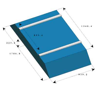
13.5.2 SiECAL Electrical Services and Cooling
A detailed integrated design of the SiECAL electrical services and of the cooling system has been developed. Figure 75 shows a close-up view of the upper side of a SiECAL barrel stave. The front-end electronics is located at the end of the readout slabs. Service cables for power supply and readout arrive at a patch panel placed on the front-side of a stave from where they are distributed to big hubs on top of each module (”Hub 1” in Fig. 75). These hubs distribute the power and readout cables further to smaller hubs from where they are finally distributed to the readout slabs. Figure 76 shows a block diagram of the electrical services for the SiECAL and the connections from ”Hub 1” via a small number of patch panels to the outside power supplies, to the common clock and the DAQ.


A conceptual design for the SiECAL cooling system is shown in Figure 77. The system foresees leakless water cooling, where a cooling station would be located outside of the ILD detector in the underground area. The water will be distributed via a hierarchical system of cooling lines (”A” to ”F”) to the barrel and endcap detectors.

13.5.3 ScECAL Electrical Services
The distribution of the electrical services for the ScECAL is very similar to the SiECAL case. Figure 78 show a block diagram of the service distributions. Also in this case, two series of hubs are planned, one for each stave and one for each column of slabs, to distribute HV and signals accordingly.

13.6 Hadronic Calorimeters Integration
13.6.1 Mechanical Integration
Two absorber structures are under study for ILD, the so-called ”TESLA” and ”Videau” structures (c.f. Figure 23). The main differences from the viewpoint of the detector integration are the mechanical behaviour, further discussed in section 14, and the layout of the detector electrical and cooling services. The analogue AHCAL and the semi-digital SDHCAL can be adapted to both mechanical structures. In practice, the AHCAL has been designed with the ”TESLA” structure in mind, while the SDHCAL is optimised for the ”Videau” case.
13.6.2 AHCAL Electrical Services and Cooling
An engineering model of the AHCAL barrel section in the ”TESLA” structure has been designed and is shown in Figure 79. Eight of these modules form a ring, two rings form the barrel detector. The active layers are read out via electronic boards that are located on the outside of the absorber structure. The data concentrators and power interfaces are accessible when the endcaps of the ILD detector are open.

A close-up of the data concentator boards, the electrical services and the cooling system is shown in Figure 80. This service concept has been implemented and successfully used with the AHCAL prototype (Figure 47). The electrical and cooling lines of the ECAL, AHCAL, the TPC and the inner detector are routed via the gaps in the AHCAL front between the barrel and the endcap detector, as shown in Figure 81.


13.6.3 SDHCAL Electrical Services and Cooling
The SDHCAL barrel detector consists of three or five rings of eight wedge-shaped modules in the Videau configuration. As the active layers are installed from the outside of the barrel structures, access requires the removal of the respective barrel rings from the detector solenoid. The cables and cooling services run on the outside of each module to the barrel front face, as shown in Figure 82. The SDHCAL services are routed around the detector solenoid to the outside. The services of the inner detector, the ECAL and the TPC can be routed on the front side of the SDHCAL barrel detector, as shown in Figure 83.
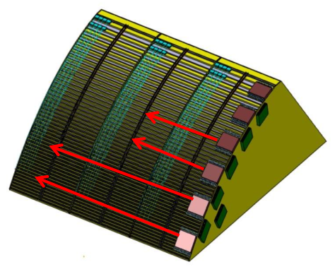

13.7 Very Forward System Integration
The very forward systems, BeamCAL, LumiCAL and LHCAL, are carried by the support structure for the final focus quadrupole QD0. Figure 84 shows the mechanical layout and the conceptual service paths of the forward calorimeters.


14 Mechanical structure studies
The mechanical behaviour of the ILD components is crucial in two respects. On the one hand, the high-precision and hermeticity of the detector requires a precise relative adjustment of subdetector components within each other, with tight tolerances at the interfaces and boundaries. These aspects were studied by simulating static deformations of the components under gravity and other constraints. On the other hand large devices in Japan must obey strict rules as regards their behaviour in case of seismic events (see section 19). This was investigated by modelling the dynamic behaviour of components, including the computation of their ”eigen modes” and their reaction to reference earthquake parameters from the foreseen ILC Kitakami site. Most of the attention has up to now been given to the calorimeter mechanical structure which governs the global stiffness of the ILD detector inside the coil.
As mentioned in section 10.2.5 two options of the hadronic calorimeter, so-called ”Videau” and ”TESLA”, are under consideration. In both cases, the electromagnetic modules are fixed to the inner plates of the hadronic wheels with two rails parallel to the z direction. Two critical aspects are of particular importance for the calorimeters: the respect of the tolerances of the thin azimutal clearance (2.5mm) between the electromagnetic modules, to avoid mutual contact and possible damage of the modules, and the flatness of the hadronic absorber plates which define the gaps in which the sensitive layers are introduced. The latter is particularly important for the SDHCAL instrumentation option since RPC’s require a high level of flatness. Both Videau and TESLA mechanical options have been simulated in detail and the results provide input for further optimization of the layouts.
Videau simulations:
The static behaviour of a full Videau calorimeter wheel was simulated with a shell model. In order to save computing time, the electromagnetic modules were approximated by a 3D solid model. This simplification was validated separately by a comparison to a single module shell model simulation. The results are shown in Figure 85: the hadronic structure turns out to be very stiff with largest deformations of a fraction of a mm. This is due to the vertical flanges of the Videau modules which strongly rigidify the overall structure. The electromagnetic modules are also only slightly distorted: the largest deformation stays below 1mm and the azimutal clearance between modules is reduced to 2.3 mm in the worst case, well within the required tolerances.
One advantage of the Videau layout is to avoid a projective dead zone at a polar angle of , but the number of dead zones in z is 4 for the baseline number of 5 wheels. One question is whether one could reduce this number of dead zones by reducing the number of wheels to 3. Mechanical simulations show that for 3 wheels it is possible to keep deformations at the boundary between the electromagnetic modules within specifications, provided the inner hadronic absorber plate thickness is slightly increased.
First dynamic simulations of the Videau structure were also performed with the computation of eigen modes. They show that the overall calorimeter barrel behaves as a rigid structure under oscillating accelerations, with little variation of the z distance between the wheels.

TESLA simulations:
In the ILD DBD the TESLA mechanical layout was initiall designed with corners at , , etc. in azimuth, which corresponded to the optimal configuration as regards mechanical stiffness. In order to facilitate the silicon sensor tiling of the ECAL endcap, the structure has since then been rotated by . Since there are no vertical disks, the behaviour of the structure now resembles that of a Roman arc.
The mechanical behaviour of the barrel structure with the new orientation has been simulated with shell and 3D models. The simulations showed deformations of up to 5 mm, requiring actions to reduce them. A minimised number of 10 mm wide additional spacers have been introduced between absorber plates in critical points – near the fixtures of the ECAL and near the supports from the cryostat – (Figure 86 left), resulting in static deformations of less than 2 mm everywhere (Figure 86 right).

The 3D model has also been used to obtain the first 200 vibration eigen modes. However, calculating the response of the system to an external excitation exceeds computational limitations and requires more advanced methods. The so-called component mode synthesis (CMS) method has been used, in which the detailed sub-structure of calorimeter modules is replaced by blocks which however preserve the overall mechanical behaviour of the module at specially configured boundaries. A simplified AHCAL model has been used to validate this model against a full 3D simulation up to the response to frequency sweeps and to real Japanese Earth quake data. The application of this model to the re-optimised AHCAL structure is in progress.
15 Coil and yoke studies
A conceptual design of the ILD solenoid, the yoke and the cryostat had been developed for the ILD DBD [115, 116]. Recently, studies have been done to optimise the engineering design of the magnet, to study the magnetic properties of the large and small ILD detector models, and to explore possible cost reductions.
15.1 Magnet Engineering Studies
A common study by KEK, Toshiba and Hitachi has been started to better understand the engineering challenges in the design and manufacturing of the ILD solenoid coil and the Anti-DID, which adds a small additional dipole field to the solenoid for better suppression of background particles in the detector (c.f. section 16 and [117]).
Figure 87 shows a conceptual design of the manufacturing process. While the three solenoid modules and the Anti-DID coils would be fabricated in industry, transportation boundary conditions require the assembly of the complete magnet on or close to the final detector site.

A case study by Toshiba concluded that the main solenoid modules can be transported on the road with the use of a specialised Jumbo Carrier while the modules of the Anti-DID would fit on a flatbed trailer (Figure 88).

Figure 89 shows a conceptual design of the Anti-DID coils and the resulting simulated dipole field with a maximum value of 0.036 T. Splitting the Anti-DID coils in four makes construction at the manufacturer and transport to the ILC site easier (c.f. Figure 88).


15.2 Field Optimisation Studies
The coil and yoke system should provide at the same time a high magnetic field in the central region and low stray field on the outside of the detector. The nominal fields for the large (small) ILD detector model are 3.5T (4T). To allow for safety margins and possible extensions to higher field values, the coil design has been developed to reach 0.5T more in each case. Figure 90 therefore shows the field map and the field distribution for the large ILD detector model and a maximum field of 4T. The corresponding distributions for the small ILD detector model are shown in Figure 91. The field maps are the result of 3D magnetic field simulations. They are implemented in the simulation tools of the detector (chapter 7) to allow for reconstruction with maximum realism when this is required by specific studies such as beam background effects (section 6.5).


The ILD detector is expected to share its experimental environment with another detector, e.g. SiD, in a push-pull scenario. This model of operations assumes that each detector can run its magnetic field while still allowing the other detector crew to work on their detector with the use of standard iron-based tools. Therefore a limit on the maximum magnetic stray fields has been agreed upon at a maximum of 5 mT at a distance of 15 m from the detector axis [32]. This requirement is the main driver for the thickness of the iron yoke of ILD. Figures 92 and 93 show the simulated stray fields for the large and the small detector model at 4 T and 4.5 T maximum central field.


Simulations have been done with different codes and the results are very consistent with an average value for the large detector of 5.60.6 mT for the maximum stray field at 15 m [120]. The stray fields for the small detector model are very similar.
The stringent limits on the stray fields are a cost issue for ILD as they drive the thickness of the iron return yoke. If the thickness would be reduced by 60 cm, the maximum stray fields at 15 m would increase to 9.3 0.8 mT but at the same time reduce the cost for the yoke by about 20% for the large ILD detector model [120].
A cost reduction of in total 50% can be reached if the iron yoke is reduced further to a thickness of 2.04 m (including gaps). The stray fields at 1 m distance from the outside of the yoke would be at the level of 100 mT which is acceptable for the operation of magnetically sensitive equipment and which is well below limits given by human safety regulations. The far stray fields in the direction of the other detector need to be shielded in that case, e.g. by using a magnetic shielding wall. Figure 94 shows the simulation of the large ILD detector model magnetic fields with a reduced yoke and a shielding wall.
Though this concept looks attractive, further studies are required. The shielding wall needs to be mobile and has to follow the push-pull movements. An engineering solution needs to be developed. Another problem is the radiation shielding. In the present design, the thick iron yoke serves as a radiation shield and allows for access to the outer side of the detector while the ILC delivers beams to the interaction region [121]. A reduced yoke might be too thin to serve for this purpose alone and additional radiation shielding, e.g. made from concrete, might need to be added.

16 Beam background studies
The ILD detector response is affected by three main sources of beam-related background: beamstrahlung emitted at the crossing point of the electron and positron bunches, halo muons produced upstream of the detector along the beamline, and low energy neutrons back-scattered from the beam dumps. Their impact on the detector occupancies has been quantified and possible mitigation investigated[122, 123]. Results are similar for both options of the ILD detector and are shown here for the large version.
16.1 Beamstrahlung
Beamstrahlung photons are radiated from the ILC beam particles in the interaction with the electromagnetic fields of the strongly focused oncoming bunches. These photons can convert to pairs with a broad energy spectrum. Most of the low-energy pairs are confined close to the z axis by the solenoid magnetic field but, due to the crossing angle between the colliding beams, a significant fraction hit the very forward detectors near the incoming and outgoing beam pipes. The central detectors are also affected, both directly by the pairs, and indirectly through back-scattering of low-energy particles from the forward detectors. It was proposed to mitigate these effects by the addition of a small dipole field to the main solenoidal field. This so-called ”anti-DID” field can be tuned to guide a large fraction of the pairs into the outgoing beampipe.
These effects have been quantified for the updated 250 GeV ILC conditions (ILC250, see Section 3), using a full simulation of the beamstrahlung particle production and of their tracking within ILD [122]. Special care has been taken to ensure stable results by adapting the GEANT4 tracking parameters to low energy particles. A realistic field map of both solenoid and anti-DID fields has been used. The response of the most affected detector, the BeamCAL, is shown in Figure 95 with and without anti-DID. A positive effect of the anti-DID is clearly visible: when the anti-DID field is applied, the particle distribution is more symmetric around the central beampipe, and the overall energy deposition in BeamCAL is reduced by about 30%.


| LAYER: | hits/BX | hits/BX | hits/BX/ |
|---|---|---|---|
| No anti-DID | anti-DID | anti-DID | |
| mean RMS | mean RMS | mean RMS | |
| VXD 1: | 1400 780 | 910 360 | 6.6 2.6 |
| VXD 2: | 970 560 | 540 210 | 4.0 1.5 |
| VXD 3: | 150 80 | 130 60 | 0.21 0.10 |
| VXD 4: | 110 60 | 110 50 | 0.18 0.09 |
| VXD 5: | 44 30 | 40 26 | 0.04 0.03 |
| VXD 6: | 39 27 | 34 24 | 0.04 0.03 |
| FTD 1: | 42 30 | 38 26 | 0.043 0.030 |
| FTD 2: | 27 19 | 24 15 | 0.029 0.019 |
| FTD 3: | 62 45 | 40 27 | 0.014 0.010 |
| FTD 4: | 42 33 | 25 17 | 0.009 0.007 |
| FTD 5: | 29 23 | 18 13 | 0.007 0.005 |
| FTD 6: | 16 13 | 9 7 | 0.004 0.003 |
| FTD 7: | 10 8 | 6 5 | 0.003 0.003 |
| SIT 1: | 51 37 | 24 16 | 0.0032 0.0023 |
| SIT 2: | 49 36 | 21 12 | 0.0029 0.0017 |
| SIT 3: | 77 56 | 34 24 | 0.0014 0.0010 |
| SIT 4: | 71 54 | 31 21 | 0.0013 0.0009 |
| SET 1: | 39 28 | 15 10 | 0.00003 0.00002 |
| SET 2: | 46 36 | 18 12 | 0.00003 0.00002 |
A similar improvement is seen for the central detectors in table 9. The most affected are the inner layers of the vertex detector, where the background is equally shared between direct hits rather uniformly distributed, and back-scattered particles showing hot spots in azimuth. Background hits further away from the beampipe are dominated by direct pairs. The anti-DID has little effect on direct hits but helps to suppress back-scattered particles and associated hot spots in the central detectors.
For the small ILD version, the overall beamstrahlung background hit rates are reduced by 10% thanks to better confinement within the beampipe by the higher solenoid field of 4T.
16.2 Halo muons
The electrons and positrons of the beam halo produce high-energy penetrating muons parallel to the beam by interacting with beamline components such as collimators. Beam simulations [31] predict that a fraction of of the incident beam electrons hit a machine component of the beam delivery system and may therefore produce muons. Five magnetized muon spoilers and one optional larger magnetized muon wall are foreseen to deviate these muons outside the ILC experimental hall. The resulting rate of muons in ILD has been simulated for ILC250 and ILC500.

Figure 96 shows the energy spectra of the muons crossing the ILD detector for the two filtering options. The muon wall significantly reduces the flux of the lower energy muons below a few 10 GeV. At ILC500 the rate of halo muons crossing ILD is of the order of 4 (resp. 0.6) muons/BX without (resp. with) the optional muon wall. At ILC250 the corresponding numbers are of the order 1 and 0.03 muons/BX for the two filtering options, respectively.
These halo muons will affect the occupancy of the detector but should be easily identified and subtracted from the physics events using topological and timing information.
16.3 Backscattered neutrons from beam dumps
A potential additional source of beam-related background consists in particles back-scattered from the electron and positron beam dumps located 300m from the interaction point in both beam directions. This background is expected to be dominated by low energy neutrons which can propagate over a long distance. Their contribution has been fully simulated with FLUKA in the context of SiD, including a detailed description of the beamline up to the beam dump as well as of the dump system itself [123]. The incoming neutron fluxes close to SiD are expected to be the same as for ILD and were interfaced to the ILD detector simulation to estimate their impact in the detector. The simulation was normalised to the dump of one full electron bunch on the +z side of the detector.
The total number of neutrons reaching the ILD detector region is found to be O() per electron bunch dump. These neutrons have very low momenta of a few 10 MeV and most of them do not deposit a detectable signal in the detector. Their propagation in ILD was simulated and the map of their stopping points in the detector is shown in Figure 97. The results are in line of what is found for SiD [123]: most neutrons are absorbed in the external layers of the ILD iron yoke, with a very small fraction reaching the external layers of the very forward calorimeters. Their energy depositions concentrate close to their stopping points: they are very small (0.1 MIP on average) and asynchronous with respect to the bunch crossings. No visible signal is seen in the ILD vertex detector and central tracker. This indicates that the neutron background should not be a critical issue within its current state of understanding.


17 Data acquisition
The ILD data acquisition takes advantage of the relatively low rate of relevant physics interactions (O(0.1 hadronic evt)/BX) and of the long idle periods between bunch trains (chapter 3) to provide a triggerless readout of the detector. The subdetector data of all BXs of a given bunch train are collected before the next bunch train and processed offline as a single data set for identification, bunch tagging and reconstruction of the individual interactions.
17.1 DAQ architecture
The overall organisation of the DAQ system is summarized in Figure 98.

The processing of subdetector data is first performed locally with a high parallelism within FPGA and ASIC boards which each typically treat O(100) subdetector channels. The individual data are zero-suppressed, amplified, time stamped and digitised, depending on the subdetector, and stored in local pipelines dimensioned adequately for a full bunch train. The ”event building” is performed between bunch trains by gathering all subdetector data of a given bunch train into a single bunch train data set. The bunch train data sets are stored locally on the IP Campus (section 6.1) and transferred to an offline computing farm which may be located on the main campus. In the farm each bunch train data set is processed individually by one processor in order to identify individual events, tag their bunch crossings and perform calibration and reconstruction. This scheme caters for the different time resolutions of the subdetectors, which range from individual bunch tagging as done e.g. in the calorimeters, to a full train integration time as in the TPC.
One critical component of the system is the clock distribution to the subdetector front-ends: this has to be done on the overall ILD detector with a precision better than 10 ps to enable time-of-flight measurements. On the other hand the overall data flow requirements are moderate. They have not changed significantly compared to the estimates reported in [2], and correspond to a raw data rate of O(100MB)/train for a storage data size of O(10PB)/year. The data flow is dominated by high granularity detectors exposed to high beam background close to the beampipe (VTX and BeamCAL). If needed it could be further reduced by local partial event processing ahead of the event building.
17.2 DAQ R&D
The front-end processing has benefited from the development of subdetector technological prototypes including final readout front-end components as reported in section 5.2. ASIC and FPGA boards with the required ILD specifications are now available for most subdetectors.
A number of common DAQ aspects relevant for the final ILD central DAQ have been developed [124] within the AIDA-2020 programme. They include both hardware and software components which have been used for different detectors or combinations of detectors in beam tests involving not only ILD prototypes but also detectors developed for the HL-LHC.
The core hardware component of the central DAQ system, the Trigger Logic Unit (TLU), provides a common interface for synchronisation and control of subdetectors. A new TLU has been developed to distribute signals to multiple detectors in beam tests. The AIDA-2020 TLU (Figure 99) has been extended over the previous version to be able to synchronise detectors with differing trigger and readout schemes, such as the CALICE calorimeters, pixel detectors and tracking devices, as well as to be able to operate at a higher particle flux. Therefore, data from different detectors corresponding to the same particle in a test beam can be combined. The TLU is used extensively in test-beam facilities at CERN and DESY and will continue to do so thereby serving the needs of many detectors also beyond ILC R&D.

Within AIDA-2020 DAQ software packages have also been developed for both data collection and monitoring. The EUDAQ2 software is an extension of the EUDAQ software developed for the EUDET pixel beam telescope. It supports detectors with different trigger schemes and different readout speeds, enabling combined beam tests of very different detectors to be performed. The software has been tested and used in several beam tests so far, notably for the AHCAL (also in conjunction with the CMS HGCAL), and for tracker modules of the ATLAS upgrade. The TLU is also fully integrated into the EUDAQ2 framework. The monitoring software, DQM4HEP, originally developed for the SDHCAL, has been used for data quality monitoring and slow control monitoring. This software is a generic development which has extendibility built in and so can be used to monitor data from any detector in any format. It has already been successfully used by the AHCAL+beam telescope and SDHCAL+SiECAL combined beam tests.
These DAQ developments have allowed multiple detectors to be more easily integrated, sparing time for understanding technical aspects of the detector technologies and the physics performances. Further detector developments will also benefit from this. The work also informs our understanding of integration and DAQ issues for the final ILD.
18 Calibration/ Alignment procedures
The ILD detector is a high-precision instrument. It can reach its designed level of performance only if the sub-systems can be fully calibrated, if the different parts can be aligned relative to each other, and if the calibration and the alignment of the system can be maintained over a long time.
For the purpose of this document all tasks which concern the internal description of a sub-detector response are defined as ”calibration”. Relative positioning of internal parts within a sub-detector, and positioning of sub-detectors relative to each other, are defined as ”alignement”.
A detailed calibration and alignment concept of the ILD detector has been presented in the letter-of-intent [1] and remains valid. Here the main arguments are repeated and their implementation updated wherever appropriate. In particular significant progress has been made since the publication of the LOI in the experimental demonstration of calibration and alignment using prototypes of the different sub-detectors.
Data play a central role in the overall calibration and alignment strategy of ILD. Particles recorded during physics running are a powerful tool for the relative alignment of different sub-detectors. They are supplemented by detailed and high precision measurements taken during the construction phase of ILD, and augmented in some cases by special data taken either from dedicated calibration or alignment systems, or in special calibration runs.
A particular challenge for ILD is the proposed push-pull scheme. Push-pull implies that the detector is frequently moved from the interaction position into a parking position, and back. Calibration and alignment need to be re-established after each move within a short time, ideally of less than a day, to minimise the loss of integrated luminosity due to re-calibration. Data also play a central role in the re-establishment of the calibration and alignment after a push-pull move. A fast re-establishment of the full calibration is only possible if external means, e.g., metrology or built in sensors, first allow a quick re-establishment of the base calibration of ILD. Based on data recorded during a normal physics run, the full calibration and alignment is then re-established and re-calculated during the physics running, without loosing additional luminosity. Only the very first part, needed to find the base-calibration would potentially result in lost data.
It is important to understand the required tolerances which are different for different sub-systems. Using a simple track model the dependence of track parameters on alignment tolerances have been studied:
- •
coherent displacement of the VTX: m;
- •
coherent displacement of the SIT: m;
- •
coherent displacement of the SET: m;
- •
coherent displacement of the TPC: m;
- •
coherent displacement of the ECAL: m;
- •
coherent displacement of the HCAL: m.
These numbers, which need to be confirmed by further more detailed studies, nevertheless issue important guidelines when optimising the different sub-detectors.
Another central ingredient into the overall precision reachable for the reconstruction is the degree of knowledge of the magnetic field in ILD. Uncertainties on the size and the direction of the field will directly translate into errors on track parameters. The field knowledge will come from two sources. First, high precision measurements of the magnetic field and its direction will be performed during the building of the detector. These measurements should be able to reach a relative precision of . Second, once data are collected stiff tracks will provide a continuous source of tracks for the further relative calibration of the magnetic field, and the correction of local distortions.
The calibration of the calorimeter systems will rely strongly on test-beam based calibration runs before installation. Independent of which technology will be selected in the end, it is envisioned that each module of both the ECAL and HCAL will be exposed to test-beam previous to installation, in order to provide a base calibration. Significant experience with prototypes over many years has shown that the calibration of the ILD calorimeter is robust over time, and can be tracked based on samples of real data.
The needs for calibration and alignment have to be taken into account from the start of the development of the overall ILD concept. The design of the mechanical structure, of the supports, and of the integration strategy all will have an impact on the calibration and alignment, and will need to be considered.
Overall it is thought that the current design and integration of ILD will allow to build a detector which can be calibrated to the required precision, aligned mostly based on data, and maintained for long times in a well calibrated and well aligned state. Nevertheless it should be noted that the detailed technical validation and demonstration of the feasibility of the different concepts is still needed before a final design of ILD can be frozen.
19 Earthquake Safety
Japan is one of most seismically active regions in the world. The proposed site for the ILC in the Kitakami mountains of northern Honshu has been especially selected putting emphasis on benign seismic conditions. Earthquake history has been taken into account as well as recent surveys on active tectonic faults. Nevertheless, earthquakes can occur and need to be taken into account. Figure 100 shows all earthquakes that were detected during 30 days in winter 2018/2019 in northern Honshu. The ILD interaction region is in the region around (39N, 141,5E).

19.1 Structural Design
Emphasis has been put on the design of the ILD detector with respect to earthquake safety in view of operability of the detector as well as disaster prevention. General rules are provided by the ISO3010 standard: ”Bases for design of structures – seismic actions on structures”. The ISO standard states two basic principles:
- •
The structure should not collapse nor experience other similar forms of structural failure due to severe earthquake ground motions that could occur at the site (ultimate limit state: ULS).
- •
The structure should withstand moderate earthquake ground motions which may be expected to occur at the site during the service life of the structure with damage within accepted limits (serviceability limit state: SLS).
The design seismic forces on mechanical structures can be determined by taking into account normalised design response spectra, weighted with load factors that take into account the respective state, ULS or SLS, local conditions and structural factors. In addition, required degrees of reliability of the structures can be taken into account.
An acceleration response spectrum for the SLS state at the Kitakami site is shown in Figure 101 for structures with different damping behaviours. In the ULS state, the accelerations are assumed to be larger by about a factor of two. These type of standard spectra serve as input for the structural studies described in section 14.

19.2 Seismic Isolation
Seismic isolation could be an attractive solution to mitigate the risk of earthquake induced accidents. Base isolation systems are in use in many cases in seismic active countries like Japan, under buildings, bridges and other critical infrastructure. A recent study [127] has explored the possibility to install seismic damping systems underneath the ILD detector, e.g. under the detector platform. Standard isolation systems consist of rubber bearings in combination with oil dampers. Figure 102(a) shows that accelerations acting on the ILD detector could be damped by a factor of 35 in case of a catastrophic earthquake. At the same time, such a system unfortunately increases the displacements of the detector in case of seismic mircrotremors that occur frequently in Japan, also at the Kitakami site (c.f. Figure 100). An extended system that adds a rigid sliding bearing could mitigate the problem. Here, friction keeps the detector coupled to the ground at lower acceleration forces. Figure 102(b) shows that no amplification of microtremors happens in that case. At the same time, the damping behaviour in case of major earthquakes is still in the order of a factor of 22 better than without base isolation (Figure 102(a)).


A seismic base isolation system underneath the detector platform could therefore mitigate seismic risks for the ILD detector. However, earthquakes could also occur when the detector is still under construction or has been opened and moved partially away from the platform. Systematic risk evaluations and the development of mitigation strategies for the full lifetime of ILD still need to be done.
20 Technical Documentation
The technical description of the ILD detector concept comprises specification and design documents as well as 3D engineering models, interface descriptions and drawings. All the documents that form the backbone of the ILD technical documentation are stored in the ILC Engineering Data Management System ILC-EDMS [128]. As this powerful system is made for experts and requires appropriate attention, an easy accessible frontend (”EDMSdirect”) has been made available. The ILD technical documentation is organised in a Work Breakdown Structure (WBS) that is mapped on a tree browser that can be accessed on the web [129]. Figure 103 shows the tree browser for the ILD technical documentation. All WBS top nodes can be expanded by clicking on them. In the Figure, this has been done for the node ”Design Integration”.

Figure 104 shows the document browser that opens for the documents stored in the EDMSdirect system. Shown here is the ”Conventions and Rules” document that belongs to the previous mentioned WBS node ”Design Integration”. A preview of the document is shown in the document browser. The document browser allows for preview of the respective documents as well as downloads of pdf or source files, depending on the authorisation of the users. Documents can be made worldwide visible as well as protected for selected users.

20.1 Interface Control Documents
The technical integration of the ILD detector is based on a set of Interface Control Documents which describe the interfaces of each subdetector to its environment:
- •
Mechanical Interface
- –
Local coordinate system
- –
Mechanical concept
- –
Critical dimensions
- –
Weights
- –
Positioning and alignment constraints
- –
- •
Electrical Interface
- –
Block and connection diagrams
- –
List of connectors
- –
Cabling and connection sheets
- –
Grounding circuits
- –
Power consumption
- –
- •
Gas and Liquid Interfaces
- •
Thermal Interfaces
- •
Test Interfaces
The Interface Control Documents are living documents that are updated as the design and understanding of the subdetector technologies advance. All documents are stored in EDMS [128] and are accessible via the treebrowser of the ILD technical documentation [129].
A dedicated document describes the ILD Conventions and Rules (c.f. Figure 104). It contains a definition of the global ILD coordinate system, unit conventions, naming and numbering conventions as well as mechanical, electrical and cooling constraints and rules. This document is also available on [129]. The interface descriptions together with the conventions and rules contain the information that has been used in creating the integrated model of the ILD detector.
Chapter 7 Physics and Detector Modelling
Accurate and detailed modelling of the physics interactions as well as the detector response are crucial for making realistic predictions about the expected physics and detector performance. The ILD software for detector simulation, reconstruction and analysis is entirely based on the common linear collider software ecosystem called iLCSoft [130]. It will be described in more detail in the next sections.
21 Modelling of ILC Conditions and Physics Processes
Large, realistic Monte Carlo samples with the full Standard Model physics () as well as various BSM scenarios have been created for the purpose of detector optimization and performance evaluation, to be presented in detail in chapter 8. The input samples for the full detector simulation are created with the Whizard [131] event generator. Whizard uses tree-level matrix elements and loop corrections to generate events with the final state partons and leptons based on a realistic beam energy spectrum, the so called hard sub-process. The hadronization into the visible final state is performed with Pythia [132] tuned to describe the LEP data. The beam energy input spectrum is created with Guinea-Pig [133], a dedicated simulation program for computing beam-beam interactions at linear colliders - see also the discussion in section 7.1. \thisfloatsetupfloatwidth=capposition=below


The two main effects of the strong beam-beam interactions are the energy loss due to beamstrahlung leading to the available luminosity spectrum (see Fig 8) and the creation of incoherent -pairs that are the source of the dominating background at the ILC. These electrons and positrons are predominantly created in a forward cone as shown in Fig 105. It is this cone that restricts the minimal allowed radius of the innermost layer of the vertex detector.
Another source of background at the ILC are events, due to beamstrahlung photons. These type of events are generated for cms-energies from to with a dedicated generator based on [134], whereas for higher energies Pythia is used.
For the large Monte Carlo data sets both backgrounds are overlaid to the actual physics event that is simulated. For the incoherent pairs, only reconstructable tracks, i.e. those that leave at least three hits in the tracking detectors, are overlaid as these constitute an irreducible background. The majority of the pair particles do not leave enough hits to be reconstructed as particle tracks and therefore give rise to a large number of seemingly uncorrelated background hits. As shown in section 25.1, these additional hits have little effect on the resulting track finding efficiency and therefore can safely be omitted for the large scale production. The situation is different for the BeamCal, which is hit by a very large number of pair particles at every bunch crossing as discussed in section 16. Here we us the detailed and complete background map for every bunch crossing, as simulated for the case of an anti-DID. events are randomly overlaid according to Poisson-distributions describing the expected number of events per bunch crossing (BX) for the four different combinations of the photon virtuality as shown in table 10. Also shown in the table are the spread of the z-position of the vertex and its mean value. It is interesting to note that the events with exactly one virtual photon have a non-zero offset of the vertex z-position. On average events per BX are overlaid.
| process type | Vertex z offset () | Vertex z sigma () | expected events per BX |
|---|---|---|---|
| WW | |||
| WB | |||
| BW | |||
| BB |
22 Detector Simulation
The main core software tools in iLCSoft used by ILD are the common event data model and persistency tool LCIO [135], the C++ application framework Marlin [136] and the recently added generic detector description toolkit DD4hep [137, 138]. DD4hep provides a single source of information for describing the detector geometry, its materials and the readout properties of individual sub detectors. Various components of DD4hep provide different functionalities. Here we use DDG4, the interface to full simulations with Geant4 [139] and DDRec the specialized view into the geometry needed for reconstruction. \thisfloatsetupfloatwidth=capposition=below


22.1 ILD Simulation Models
For detector optimization studies two ILD simulation models, ILD_l5_v02 (large) and ILD_s5_v02 (small) with the dimensions described in tables 3 and 4, have been implemented using DD4hep and released in a dedicated software package, lcgeo [140]. Note that for simplicity in the remainder of this document these two simulation models are referred to as IDR-L and IDR-S. A quadrant view of the large simulation model is shown in Fig. 106(a) together with a plot of simulated hits in the large and small detector model for comparison in Fig. 106(b). The main differences between the two models (see chapter 4) are the reduced radii of the TPC, the barrels of Ecal, Hcal, Yoke and the Coil and the increased B-field of for the small model, compared to for the large model. All other detector dimensions, in particular the longitudinal extents, and all material thicknesses have not been modified. Thus, the two models have a different aspect ratio. Detailed B-field maps with and without anti-DID have been created for both models and were used in the background studies presented in section 16. For the benchmark performance studies shown in chapter 8 simplified solenoidal B-fields are used instead. Considerable effort has been invested into making the ILD simulation models as realistic as possible, in particular by
- •
following the exact dimensions and layout of detector elements from engineering models
- •
implementing correct material properties
- •
implementing precise descriptions of the actual detector technology
- •
adding realistic amounts of dead material from supports and services, such as cables and cooling pipes
- •
introducing realistic gaps and imperfections into the subdetectors
Great care has been taken to include realistic material estimates, established by the detector R&D groups, in particular in the tracking region where the material budget has a direct impact on the detector performance. As pointed out above, this includes dead material from supports and services. Fig. 107(a) shows the material budget in the ILD tracking volume resulting from the individual tracking subdetectors including dead material and services. The spike at the edge of the tracking fiducial volume at is due to the shallow crossing of cables routed along the conical part the beam pipe. Fig. 107(b) shows the material distribution in the inner tracking region close to the IP.
floatwidth=capposition=below

22.2 Hybrid Simulation
In order to be able to study and compare the different calorimeter technologies proposed for ILD (see sections 11.4 and 11.5) hybrid simulation models have been implemented for the ILD simulation models, where two different readout technologies are implemented in the gaps of the sandwich absorber structure as shown in Fig. 108(a).

In this approach the respective other technology replaces the electronics and services present in the gaps in a real calorimeter, resulting in a very similar material budget in the passive part of the layer. The calorimeter shower development is additionally, almost entirely dominated by the absorber structure. Therefore, this approach provides results that are equivalent to the stand alone simulation of each individual technology to better than 1%, as shown in Fig. 108(b) for the longitudinal shower profile. Equivalent results have been obtained for other parameters, such as the total number of hits and the transverse shower profile. With this approach one can simulate a large set of Monte Carlo events for several calorimeter technologies using only little more CPU time than would be needed for simulating just one technology choice and at the same time one can compare different technologies with identical physics events. This hybrid simulation scheme has been implemented for the HCAL with the options of scintillator and RPC based readout as well as for the ECAL with the options of silicon and scintillator based readout.
23 Event Reconstruction
The detailed simulation with Geant4 provides hit objects with the exact amount and position of energy depositions in individual sensitive detector elements, such as silicon pixels or calorimeter cells. In the Digitization step all relevant effects from the detector technology and the readout electronics are applied to the simulated hits.
23.1 Digitization
For silicon strip-and pixel detectors as well as the ILD-TPC, the hit positions are smeared according to resolutions that have been established from test beam campaigns for the different sensor technologies, thereby including effects from charge sharing, clustering and position reconstruction. Table 11 shows the point resolution parameters used in the current ILD simulation models.
| Subdetector | Point Resolution | ||
| VTX | (layers 1-6) | ||
| SIT | (layers 1-4) | ||
| SET | (layers 1-2, ) | ||
| (layers 1-2) | |||
| (layers 3-7, ) | |||
| TPC | |||
| where and are the azimuthal and | |||
| polar angle of the track direction | |||
All point-resolutions have been demonstrated in test beams or reflect the current state of the art. In the TPC hit digitization, simulated hits that are closer than the established double-hit resolution of 2 mm in and 5 mm in are merged into one. For the silicon detectors this treatment is not necessary, due to the expected low occupancies. During the calorimeter digitization two calibration factors are applied to every simulated calorimeter hit:
- •
first, the deposited energy is normalized to the mean energy deposited by a minimum ionizing particle (MIP) in this particular calorimeter sub detector
- •
then the deposited, i.e. visible, energy in units of MIPs is converted to a total cell energy in , such that the sum of all hit energies corresponds to the incident particle’s energy
The calibration of these factors is an iterative procedure. In a first step, the mean energy deposited by MIPs is computed from single -events. In a second step, single particle events with and at are simulated and fully reconstructed with the particle flow algorithm and the resulting energy is used to compute updated calibration factors. This last step is repeated until the reconstructed energy agrees with the true particle energy to within a given margin. Different from the MC samples produced in the context of the DBD [2], Birks’ Law, describing the non-linear light yield at large loss rates in scintillator-based calorimeters, has not been applied during the production of the IDR-L and IDR-S MC samples due to a technical issue. Previous studies have shown that the effect on the energy resolution is very small and therefore there is no effect on the comparison of the two detector models expected. Dedicated digitizers take into account effects of non-uniformity of the light yield for scintillators as well as cross-talk between neighboring channels.
23.2 Track reconstruction
The ILD track reconstruction is described in more detail in [141]. The pattern recognition step is carried out independently in three regions, the:
- •
inner Si-trackers VTX and SIT ( and partly FTD)
brute-force triplet seeding followed by a road search using extrapolations to the next layer - •
forward Si-tracker: FTD
a Cellular-Automaton finding many track candidates; reduced to a unique and consistent set through the use of a Hopfield Network. - •
TPC
topological clustering in the outer TPC pad row layers for seeding, followed by a Kalman-Filter based road search inwards
In a final step the track candidates and segments are combined into a unique set and then, after assignment of left-over hits, a final refit is performed with a Kalman filter. The correct reconstruction of the kinematics of charged particles requires a sufficiently detailed description of the material the particles have traversed in order to correctly account for effects of energy-loss and multiple-scattering in the fit. The DD4hep component DDRec provides dedicated surface classes for track reconstruction and fitting. These surface classes provide the geometric information of the corresponding measurement surfaces as well as material properties, averaged automatically from the detailed model. Surfaces are also used to account for effects from dead material layers, such as support structures or cables and services. Fig. 109 shows the tracking surfaces used for the inner tracking detectors of ILD.


23.3 Particle Flow
After the reconstruction of charged particle tracks the particle flow algorithm (PFA) is applied to reconstruct particle showers in the calorimeters. PFA aims at reconstructing every individual particle created in the event taking the best available measurement for each given type, i.e.:
- •
charged particles
using the momentum measured in the tracking detectors with the excellent resolution described in sec. 25 - •
photons
measured in the ECAL with an energy resolution of - •
neutral hadrons
measured predominantly in the HCAL11 1 hadronic showers often start in the ECAL and might extend into the Muon system - this is taken into account in PandorPFA with an energy resolution of
The best jet energy measurement in hadronic events would be achieved if the above algorithm would work perfectly. However in reality there is always confusion in the assignment of individual CalorimeterHits to Clusters and showers as well as in the assignment of tracks to clusters. The best PFA implementation to date is PandoraPFA [142], interfaced to Marlin in a dedicated package DDMarlinPandora. The ILD reconstruction with Pandora also utilizes the instrumented return yoke and the forward calorimeters. The input to PandoraPFA are the reconstructed tracks, candidates for kinks and s as well as all digitized calorimeter hits. A number of sophisticated clustering algorithms are then applied in an iterative way, thereby optimizing the track-cluster matching based on the momentum-energy consistency. The output of PandoraPFA is a list of reconstructed particles, typically referred to as particle flow objects (PFO).
23.4 High Level Reconstruction
After having reconstructed all the individual particles in the event, the next step in the processing is the reconstruction of primary and secondary vertices. This is carried out in iLCSoft with the LCFIPlus [143] package. The primary vertex of the event is found in a tear-down procedure, starting with all tracks and gradually removing tracks with the largest -contribution, up to a given -threshold. Thereby, the constraints from the expected beam spot are taken into account . In a second step LCFIPlus tries to identify secondary vertices, applying suitable requirements for invariant masses, momentum directions and s. Secondary vertices and optionally isolated leptons can be used by LCFIPlus for jet clustering, aiming at high efficiency for correctly identifying heavy flavor jets. The actual jet clustering is then performed by using a cone-based clustering with a Durham-like algorithm [144]. Alternatively users can use jet clustering algorithms from the Fastjet [145] library that is interfaced to Marlin in a dedicated package MarlinFastJet. LCFIPlus also provides algorithms for jet flavor tagging using boosted decision trees (BDTs) based on suitable variables from tracks and vertices. A palette of additional high level reconstruction algorithms is used for physics analyses:
- •
particle identification using dE/dx, shower shapes and multi-variate methods
- •
-finders for the identification of and -mesons
- •
reconstructed particle to Monte-Carlo truth linker for cross checking analysis and reconstruction efficiencies
- •
tools for jet clustering using Monte-Carlo truth information
- •
processors for the computation of various event shapes
24 Monte Carlo Production on the Grid
The linear collider community uses the ILCDirac [146] toolkit for large scale Monte Carlo production on the Grid. ILCDirac is highly configurable and ILD uses a dedicated production chain [147], a schematic view of which is shown in Fig. 110. The Monte Carlo production is split into four main steps:
- •
GenSplit
Split generator file to many files with small number of event files so that simulation and reconstruction jobs complete in adequate CPU time and produce a managable size of output files. This has the advantage that the same input files can also be used for fast simulation programs such as SGV [148]. - •
Simulation
Simulation of the detector response to the particles generated in the events using ddsim. ddsim is a python application that uses the Geant4 gateway DDG4 together with the detailed detector simulation model. - •
Reconstruction
Full event reconstruction with the algorithms described in sec. 23, writing out detailed REC-files with all available information, including digitized hits and a much reduced DST-file format. - •
Merging of DST files
The rather small DST-files are merged into larger files for easier handling.
In order to investigate the effect of reducing the detector dimensions on the physics performance, two large Monte Carlo data sets for the large and small ILD simulation models have been produced. The produced data sets correspond roughly to at with the exact numbers of events processed for the different classes shown in table 12.
| event class | description | events processed |
| 2f | two fermion final states | |
| 4f | four fermion final states | |
| 5f | five fermion final states | |
| 6f | six fermion final states | |
| aa_4f | two fermion by interaction | |
| higgs | higgs process | |
| np | new physics process | |
| aa_lowpt | background | |
| seeablepairs | -pair background | BXs |
| calibration | single particle, events | |
| 6f(WW) | dedicated 6f sample at |
floatwidth=capposition=below

Chapter 8 Detector and Physics Performance
The overall performance of the ILD detector is a combination of the excellent resolutions and efficiencies of the individual sub-detectors and the sophisticated reconstruction and analysis algorithms described in the previous chapter. This chapter reviews the ILD performance, beginning with the pure system performance that is achieved from reconstructing individual long lived particles, followed by the high-level reconstruction of jets and physics objects, ending with selected detector physics benchmarks. Where applicable this performance is presented for the large (IDR-L) and the small (IDR-S) detector models. Unless stated otherwise, the silicon based readout option for the ECAL and the scintillator based readout option for the HCAL of the hybrid simulation described in section 22.2 have been used in the event reconstruction.
25 System performance
25.1 Tracking
The efficient identification and precise reconstruction of charged particle tracks is crucial for the overall physics performance of the ILD detector. The goal for the asymptotic momentum resolution [149] is
ensuring that the Higgs mass measurement from events is dominated by the beam energy spread rather than the detector resolution.
To evaluate the tracking resolution of the ILD detector models, samples of single -events at fixed momenta (p= ) and polar angles () have been run through the full simulation and reconstruction as described in sections 22 and 23 with the single point resolutions given in table 11. Fig. 111 shows the results for the inverse transverse momentum resolution and the impact parameter resolutions and in the -plane and along the -axis respectively for the large and small detector models ILD-L and ILD-S. The performance goal for the asymptotic momentum resolution is met by both detector modes as can be seen in Fig. 111(a). Fig. 111(b) shows the ratio of the resolution for the small and large detector. In the barrel region the larger detector is slightly better, due to the larger number of hits and the corresponding larger lever arm, despite the lower B-field. In the forward region this behaviour is reversed as here the same number of hits are available due to the identical detector geometry in this region and it is the higher B-field that causes a better measurement of the curvature and thus the momentum. The impact parameter resolutions for the large and small detector models are equal to within a few percent, as can be seen from Fig. 111(d) and 111(f), except at low momenta in the forward region, where the large detector is better, as here the higher B-field and increased curvature lead to a reduced lever arm for the small detector. In the barrel region, one observes very similar resolutions for the impact parameter in the -plane and that along the -axis, whereas in the forward region, where less VTX-hits contribute, is significantly worse than (see Fig. 111(c) and 111(e))


The track finding efficiency of the algorithms described in section 23 is evaluated with -events at fully simulated and reconstructed for both detector models. The tracking efficiency is defined as the ratio of the number of correctly reconstructed tracks with a hit purity higher than 75 % to the number of Monte Carlo tracks that are created within of the IP, left at least 4 hits in the detector and did not decay in flight. The resulting efficiency is shown in Fig. 112 as a function of momentum in (a), transverse momentum in (b) and ) in (c). As can be seen in (c), the tracking is almost perfect for particles with and down to and better than 99 % in the very forward direction. At low momenta and in the forward direction, the small detector performs slightly worse than the larger variant, which is due to the larger B-field that causes larger curvatures of the tracks. In the barrel region some of this effect could potentially be alleviated by moving the innermost layer of the vertex closer to the beam, which would be possible as the background cone from pair particles is also forced to lower radii by the higher B-field.
The qualitative dependency of the efficiency on momentum and polar angle together is shown in the 2D plots (e) and (f) for the large detector model. The efficiency is flat as a function of transverse momentum in all but the very forward () part and almost perfect above , also in that region. This is expected as the track finding in this region has to be done across several sub-detectors (VTX, SIT, FTD) with mixed barrel and disk layouts, naturally leading to slightly larger inefficiencies. An optimization of the geometrical layout of the inner silicon tracking detectors for ILD with respect to an improved pattern recognition capability would be the subject of future studies. A small inefficiency persists in the very forward region also for higher momenta. The above studies have been done with the same background overlaid as for the large Monte Carlo samples. In (d) the tracking efficiency is shown also with complete and detailed simulations of one and two bunch crossings of pair background overlaid. Only a very small degradation of the tracking efficiency at the lowest momenta is observed.
25.2 Particle Flow performance and JER
The performance of the Particle Flow Algorithm (PFA) is evaluated with dedicated -events, , where the is chosen to have the desired mass of twice the jet energy and decays at rest. This allows to distinguish the measurement of the actual jet energy resolution (JER) from other effects like ISR-photons or confusion in jet clustering that occur in more complex, realistic events.
The jet energy resolution is then evaluated as
| (1) |
The is defined to be the of the central of the distribution and the is its mean value. This measure is robust against large tails and should be multiplied by a factor of to obtain an equivalent Gaussian analyzing power[150]. Fig. 113(a) shows the JER as a function of the jet energy for selected energies for the large and small detector model in the barrel region () . For the resolution is better than 4% and approaches 3% (3.2%) for the large (small) model at higher energies. In the forward region () the JER is slightly worse and the difference between large and small detector is less pronounced as can bee seen in Fig. 113(b). In order to ensure that the jets are fully contained in the acceptance of the detector, an additional cut of is applied. The JER as a function of the polar angle of the jets (the thrust-axis of the di-quark events) is shown in Fig. 113(c) for the large detector model. The observed dependency is rather flat throughout the barrel region, increasing somewhat after the barrel-end-cap transition with a visible rise in the very forward region, similar for all energies. The effect of heavy flavor quarks on the jet energy resolution is shown in Fig. 113(d), where the resolutions is plotted for di-quark events together with and events for the large model. The observed degradation in the JER for the heavy quark jets can be fully attributed to the missing energy carried by neutrinos, as can be seen from the dashed lines, were the energy is corrected for the -energies using Monte Carlo truth information. The linearity of the jet energy measurement is shown in Fig. 113(e) to be better than 5% in the barrel region.
25.3 Vertexing
The correct identification of heavy flavour decays in jets requires a precise measurement of the coordinates of secondary vertices. The vertex resolution is studied with the dedicated events that are also used for the flavour tagging training and performance studies, described in section 26.1. The resolution is measured along the longitudinal direction of the jet and two transverse directions and , defined as:
| (2) |
whith the 3-momentum of the -quark taken from Monte Carlo truth. The result is shown for the transverse (a) and longitudinal (b) components of the secondary vertices as a function of the distance from the in Fig. 114.
Fig. 114(c) shows the resolution of the primary vertex’ z-position as a function of the number of associated tracks. The resolution is better than for low multiplicity events and approaches for high multiplicity events. The radial component of the primary vertex is already known extremely well from the beam-spot position to . The overall vertexing performance for the large and small detector models is very similar, as expected already from the single track impact parameter resolutions shown in Fig. 111 (c)-(f).
25.4 Charged Particle identification
Measuring the energy loss of charged particles in the ILD-TPC provides a powerful tool for identifying the type of the particle.

Fig. 115 shows the reconstructed from a truncated mean for charged particle tracks in the TPC as a function of the particle momentum, clearly revealing the bands of the most abundant particle types and . By fitting Gaussian distributions, with mean and standard deviation , to individual bands in momentum bins one can define a separation power for distinguishing the two particle types A and B:
| (3) |
Figure 116 shows the separation power for and based on the measurement in the TPC of the large and small detector model (a) and the possible improvement that could be achieved by combining it with a time-of-flight (TOF) measurement in the large detector (b). As a proof of concept a possible TOF estimator is computed here. It uses the first ten calorimeter hits in the Ecal that are closest to the straight line, resulting from extrapolation of the particle’s momentum into the calorimeter, assuming an individual time resolution of ps per hit22 2 While this time resolution seems realisticly possible, it has to be noted, that so far it has not yet been demonstrated in a test beam prototype.. The results optained clearly motivate further studies on timing measurements and optimised TOF estimators in the ILD calorimeters.
An example in the context of physics analyses can be seen in Fig. 117. It compares the performance of the charged Kaon identification based on for the large and small detector models, as obtained from the and benchmarks described in Sec. 27.9 and 27.10, respectively. For the same efficiency, the large detector reaches a higher purity due to its larger TPC radius, which results in a better resolution.
floatwidth=\SfigwFull,capposition=beside
Additional methods for charged particle identification using calorimeter shower shapes have also been developed and used in specific physics analyses.
25.5 BeamCal reconstruction
Many analyses require the efficient measurement of electromagnetic showers at small polar angles in the BeamCal. Due to the large amounts of background from pair particles (c.f. 16), the BeamCal requires a special reconstruction algorithm for identifying showers in the presence of background. Fig. 118(a) shows the achieved reconstruction efficiency for single photons for the large and small detector models for and respectively. Due to the significantly larger backgrounds at the efficiency rises slower with polar angle than at and there is almost no difference observed between the two models. In contrast at lower center of mass energy the small detector shows better performance, as expected due to the reduced background as an effect of the higher B-field. Here a plateau of the efficiency at is reached between and due to the keyhole opening of the BeamCal front face. Fig. 118(b) shows the fraction of clusters that are falsely reconstructed from background hits (1-purity) as a function of the polar angle. It is at most 1% in the region of low efficiency and drops to below one permille in the region where the full efficiency is reached.
26 High-level Reconstruction Performance
26.1 Flavour-Tag Performance
The efficient identification of heavy flavour jets in hadronic events is an indispensable ingredient to many important physics analyses, such as the and branching ratio measurements. The LCFIPlus tool, described in section 23.4, is used for flavour tagging with BDTs. The training of the BDTs is done with events at , where all quarks are chosen to have the same flavour, mostly from events. The jets are predominantly produced in the central region of the detector in these events at the given center of mass energy. The performance is evaluated with a sub-sample of the same type of events that has not been used for training the BDT. The resulting performance is shown in Fig. 119 for the large and small ILD detector model. In (a) the background rate as a function of the c-tagging efficiency for b-quark and light flavour quark jets is plotted and (b) shows the background rate for c-quark and light flavour quark jets as a function of the b-tagging efficiency.
As expected from the impact parameter and vertex resolutions there are no significant differences observed between the large and small ILD variants for the flavour tagging performance. The flavour tagging performance has been seen to vary with the jet energy and jet multiplicity [143]. The optimal performance in a physics study can be achieved by retraining the BDTs for the corresponding signal event topology.
26.2 Hadronically decaying ID
The correct identification of lepton decay modes is of particular importance in the extraction of observables sensitive to the lepton spin direction: examples are measurements of the polarisation and Higgs CP based on spin correlations in decays. Hadronic decays typically offer the highest sensitivity to the spin, due the presence of a single neutrino. The identification of these hadronic decay modes can be factorised into the charged and neutral components. We focus here in particular on understanding the identification of the neutral part, which consists largely of photons from neutral pion (and to a lesser extent other neutral meson) decays. In the decays of highly boosted taus, these photons are typically rather close to both a charged particle and one or more additional photons produced in the same decay. The separation between these photons in the calorimeter depends on its inner radius, while the distance to charged particles additionally depends on the magnetic field strength. We can therefore expect some differences in performance for the large and small ILD detector models.
The performance of decay mode identification was studied in -pair production events at a centre-of-mass energy of GeV. These very highly boosted decays are the most challenging to reconstruct due to the small distance between particles in the highly collimated decay jets. The standard ILD reconstruction algorithms were applied to these events.
In each event, two high momentum, back-to-back, charged particle flow objects (PFOs) were identified as jet ”seeds”. Figure 120 shows the number of photon PFOs identified in a cone around these seed tracks, in the case when the lepton decayed to . In these events, exactly two photons are expected in the vast majority of cases. The distribution shows that it is challenging to reconstruct both photons: in around half of the cases only a single photon cluster was reconstructed, which is due to the merging of the two photons into a single reconstructed particle. A difference is seen between the two detector models, with the large version somewhat more often correctly resolving the two photons, which can be understood as being due to the larger ECAL radius increasing the distance between the photons’ electromagnetic showers.
A simple cut-based approach to the identification of single-prong hadronic decays was developed, based on the number of reconstructed photon PFOs, and the invariant mass of this set of photon PFOs both alone and together with the charged PFO around which the candidate jet was built. The ability of this algorithm to distinguish (””), (””), and (””) decays is shown in Fig. 120. The product of selection efficiency and purity varies between around 30% and 75% among these three decay modes. The large detector model performs slightly better, as expected thanks to the larger inner ECAL radius.
26.3 reconstruction
With the excellent particle flow, particle identification and vertexing capabilities of ILD discussed in the previous sections, there is a great potential to reconstruct various exclusive decay chains of short-lived baryons and mesons. This is of special interest in case the ILC will be operated at the pole, but also at higher energies we expect further improvements to flavour tagging and jet energy resolution once this potential is fully exploited in reconstruction and analyses. This is an area where new algorithmic developments could still lead to a significant improvement of the ILD performance.
At the current stage, we only provide a very simple example as a proof of principle, namely the reconstruction of decays. Due to its extremely well-known mass (known to 3.6 ppm [151]), the is an important standard candle, e.g. for calibration of the tracker momentum scale.
Figure 121 shows the invariant mass spectrum of reconstructed muon pairs in the region, comparing the large and small detector. All available SM MC events from the optimisation production at GeV (c.f. Sec. 7) have been used and weighted to the ILC500 conditions as defined in Sec. 27.1. The combinatorial background has been determined from like-sign muon pairs and has been subtracted from the opposite-sign pairs, leading to the fluctuations around zero in the off-peak regions. At GeV, most candidates are produced in the forward direction, with and at rather low transverse momenta, typically below GeV. Due to the larger -field, the small detector has a smaller acceptance at low than the large detector, with about k vs k recontructed ’s compared to about k available at generator level. On the other hand, the better momentum resolution of the small detector in the forward region leads to a more narrow peak.
27 Physics Benchmarks
The performance of the two ILD detector models IDR-L and IDR-S has been evaluated on a number of physics benchmarks discussed in this section. Despite the fact that a 250-GeV version of the ILC is currently under political consideration in Japan, the detector benchmarking has been performed at higher center-of-mass energies, mostly at 500 GeV, and in one case even at 1 TeV. This choice has been made in order to make sure that both detector models perform adequately also under the more challenging experimental conditions of the higher energy stages, and in order to cover e.g. a wider range of jet, lepton and photon energies.
The benchmarks presented in this section have been chosen to illustrate many performance aspects with a minimum number of physics channels, and are not meant to cover the complete physics case. The main focus of the analysis work was not always the pure optimisation for utmost physics performance, but rather to better understand and highlight the role of individual performance aspects and their interplay. For all benchmarks, the MC samples described in Sec. 7 have been used. In particular, the low hadron as well as pair background in the detector acceptance has been overlaid as described in Sec. 21.
Unless stated otherwise, the analyses performed for and since the time of the DBD remain valid in their physics message. For an up-to-date review of the ILC physics case, based on ILD detector simulations, see e.g. [8].
27.1 Luminosity, Energy and Polarisation for the Physics Benchmarks
The benchmark studies are based on the Monte-Carlo samples created with the conditions and software described in Sec. 7. About 150 million events have been produced in total as detailed in Tab. 12.
All results have been scaled to the integrated luminosity and beam polarisation of the full H20 running scenario originally defined in [8], which is — for the higher center-of-mass energies — unchanged since [25]. In particular, the H20 scenario comprises 4 ab-1 at 500 GeV, with beam polarisation absolute values of 80% for the electron and 30% for the positron beam. The total luminosity is shared between the different polarisation sign combinations according to . This configuration is referred to as ILC500 in the following. Analoguously, 8 ab-1 are considered at 1 TeV, with absolute polarisation values of 80% for the electron and 20% for the positron beam, with the same sharing. This configuration is referred to as ILC1000 in the following.
27.2 Hadronic Branching Ratios of the Higgs Boson
The determination of the branching ratios of the Higgs boson into , and in particular to is one of the unique items on the menu of future colliders. These measurements crucially depend on an excellent flavour tag, c.f. Sec. 26.1, enabled by vertex detectors with micrometer point resolution and a first layer placed as close as 1.6 cm to the beam line, as well as the tiny, nanometer size beam spot of the ILC. The full performance of the ILC on Higgs branching ratio measurements, combining all final states, can be found in [8].
As a benchmark, the final state, including both the dominant contribution from fusion as well as a small contribution from , was chosen in order to minimize the impact of other performance aspects like e.g. jet clustering. Thus the target physics observable here is . With the full 500 GeV data set, about 200000 events would be produced in this final state alone, while about 30000 and 10000 and would be available, respectively. In the limit of 100% signal efficiency and zero background, this would correspond to statistical precisions on of 0.2%, 0.6% and 1% for , and , respectively.
The benchmark analysis is documented in detail in [152], and follows earlier analyses [153, 154, 155]. After a cut-based preselection, the kinematic selection of events is refined by a multi-variate approach. Up to this point, no flavour-tag information is used. Figure 122 shows the distributions of the reconstructed Higgs mass at this stage of the analysis for the signal on top of the remaining SM backgrounds, comparing both detector models. In this plot, the relative normalisation of signal and background is given by the respective cross sections, but the total histograms for have been normalised to an integral of in order to allow a shape comparison between IDR-L and IDR-S.
Figure 123 shows the 2D distributions of - vs -likeliness (c.f. Sec. 26.1) for the different Higgs decay modes. The -likeliness (for , or ) is obtained by combining the flavour tag output for the two individual jets, and , according to
| (4) |
The “data” distribution is then fitted in 3D template approach in order to determine the contained fractions of the various hadronic Higgs decay modes, where the 3rd dimension is the -likeliness. Due to the limited available statistics of background MC, a much smaller number of bins than displayed in Fig. 123 was used [152]. The resulting precisions from this template fit are displayed in Fig. 124. Fig. 124(a) shows the actual results for IDR-L and IDR-S with the data only. For comparison, the corresponding result obtained for a perfect flavour tag is also displayed. The comparison shows that for and , the current flavour tag performance yields a close to perfect identification of these final states. For , however, the real flavour tag performs worse by a factor of two. On the other hand, for a worse flavour separation, especially the expected precision for degrades rapidly [152], thus the performance of the ILD detector and reconstruction is crucial for the ability to measure .
Figure 124(b) finally compares for IDR-L and IDR-S the precisions combined over all data sets of ILC500 as defined in Sec. 27.1. It shows a rather equivalent performance of both detector models. In the case of , which is most sensitive to the detector performance, the smaller detector model actually performs a little better: Due to the stronger magnetic field of IDR-S, less tracks from low- hadron overlay are reconstructed, which helps the charm tag to perform a bit better.
27.3 Higgs Mass from
The single most precise method to measure the Higgs mass is the recoil analysis at GeV [9], for which a precision of MeV has been projected for the full ILC250 data set [156]. At much higher than the production threshold, the recoil technique suffers substantially from the increasing amount of ISR and beamstrahlung. In addition, the momenta of the muons from increase in magnitude and thus are measured less precisely. Still, the data collected at higher centre-of-mass energies can be exploited effectively when using the fully-reconstructable decay modes of the Higgs boson in combination with kinematic constraints33 3 In direction the initial momentum is not zero due to the crossing angle of the beams, but given by . from the known initial state. E.g. the constraints and GeV can replace the measured energies of the Higgs decay products, so that only the angles of the Higgs decay products and the momenta of the muons from enter in the mass reconstruction. Thus the technique is independent of systematic uncertainties as e.g. associated with the -jet energy scale. The detailed description of the technique can be found in [157].
The resolutions on the kinematic quantities which enter the Higgs mass reconstruction, namely azimuthal and polar angles of the jets and the muon energy, are compared in Figs. 125(a) and 126 for IDR-L and IDR-S. For this, the jet angles obtained from clustering the MC particles after hadronisation serve as truth reference, so that the detector performance is singled out from other influences. Figure 125(b) illustrates the effect of hadronisation by comparing to the quark-level direction taking IDR-L as example. It shows that the detector resolution (blue histogram, same as in Fig. 125(a)) is comparable, but smaller than the hadronisation effect (red histogram). While the angular resolutions are very similar for both detector models, the muon energy resolution is worse for the small detector, reflecting the somewhat worse resolution for high-momentum tracks in the central region of the detector, c.f. Fig. 111.
Figure 127 shows the propagation of this effect to the actual physics observable, i.e. the reconstructed mass of the Higgs candidates. IDR-L and IDR-S are compared for the muon channel in Fig. 127(a) and for the electron channel in Fig. 127(b). In both cases signal and all backgrounds from the SM and other modes are combined, with clear peaks visible around the nominal Higgs and boson masses. In particular in the muon channel, the worse momentum resolution of the small detector leads to the peaks being visibly wider. The uncertainty on the Higgs mass is extracted by fitting these distributions following the approach used for the recoil analysis [9]. For ILC500 as defined in Sec. 27.1, this results in an uncertainty on the measured Higgs mass of MeV in the case of IDR-L and MeV for IDR-S, an increase of about .
27.4 Branching Ratio of
In the SM, the decay of the Higgs boson into a pair of muons is a very rare decay, with a branching ratio of . In order to identify this small signal, the achievable mass resolution, thus the precision to which the momenta of the two muons are measured, plays a crucial role. For the purpose of detector benchmarking, we consider only as observable, which isolates best the effect of the muon momentum resolution. At center-of-mass energies above GeV, the channel gives the leading contribution to the combined result, while at GeV dominates. The ILD result for combining all channels at GeV and GeV, based on DBD MC samples, can be found in [158].
The selection [159] targets events with substantial missing four-momentum plus two well-reconstructed, oppositely charged muons. Kinematic and angular variables are exploited in an MVA analysis. Figure 128(a) shows the di-muon invariant mass distribution for all selected signal events. In case of the small detector model, the mass peak is about wider than for the large detector. This originates from the combination of the muons from the Higgs decay being highly energetic and rather central, plus the better momentum resolution of the large detector for high-momentum tracks in the barrel. This effect is seen more clearly in Fig. 128(b), which compares the event-by-event uncertainty of the di-muon invariant mass, as calculated from the track covariance matrices, for the selected signal events with both muons in the barrel region of the detector ().
For the GeV data set of the H20 scenario, the asymptotic precision on cross section times branching ratio for the case of efficiency and no backgrounds would be 13%.
After the event selection, about signal events, corresponding to a selection efficiency of , remain over a evenly distributed background of about events (counted in a mass window between and GeV) for ILC500 as defined in Sec. 27.1. Finally, the expectation values for the number of signal events observable above the backgrounds as well as for its uncertainty are obtained from many toy MC fits to the di-muon invariant mass spectrum [159]. The obtained precisions on are % for IDR-L and % for IDR-S. The relative difference of is consistent with the expectation of a difference in the signal peak width over a flat background. Either number, however, is about a factor worse than the asymptotic precision for the case of efficiency and no backgrounds, which would be 13%. The difference is vastly dominanted by the remaining “irreducible” backgrounds with two muons and two neutrinos from pairs decaying either directly to muons or via tau-leptons. While there is certainly room for improvement in rejecting these backgrounds, this will factorize from the impact of the signal peak width, as long as the background remains flat in the discriminating variable.
27.5 Sensitivity to invisible
The decay of the Higgs boson into invisible particles is of particular interest because it could give important clues about the nature of Dark Matter. As a detector benchmark for testing the impact of the jet energy resolution, in particular the hadronic decay mode of the boson is considered here. Thus the physics observable will be the upper limit on .
The event selection [160] targets events which are consistent with a di-jet plus missing four-momentum topology, where the di-jet invariant mass should be compatible with the boson mass. The jet finding step also serves to reject PFOs from overlay of low- hadron events. The final discriminating variable is the invariant mass of the “invisible” four-momentum recoiling against the boson.
Figure 129(a) shows the di-jet invariant mass for the selected signal events at various levels of realism from the full reconstruction to cheating all effects apart from the detector and particle flow performance. The first step of partial cheating removes jets with semileptonic heavy flavour decays. In a detector like ILD shower shapes in the highly-granular calorimeter and specific energy loss information from the TPC should allow an excellent identification of leptons in jets, which, combined with secondary vertex information should allow to significantly improve scale and resolution for heavy flavour jets with semileptonic decays. However, the corresponding reconstruction algorithms are still under development and thus could not be applied here. Similarly, work is ongoing to improve the removal of overlay backgrounds, see e.g. Sec. 27.12 and Ref. [161]. Thus, we expect that with future reconstruction improvements, a performance similar to the case “w/o sld and overlay” could be reached. The beam spectrum (BS) by construction does not affect the invariant di-jet mass. ISR, on the contrary, can lead to photons in the detector. In this analysis, no attempt has been made to identify the corresponding particle flow objects. Therefore, also a large part of the effect of ISR on the di-jet mass should be recoverable with a more sophisticated analysis.
The corresponding situation for the recoil mass is shown in Fig. 129(b). Here, ISR and BS have a large impact since they lead to a deviation of the actual initial state of the hard interaction from the naive assumption. Since this effect is dominated by photons from ISR and BS which escape undetected along the beam pipe, no attempt has been made to correct the kinematics of those events in which a photon is detected. See e.g. Sec. 27.11 for an analysis where such a correction is applied.
The recoil mass distributions obtained with the large and small detector model are compared in Fig. 130. Fig. 130(b) shows the situation at the current full reconstruction level, while Fig. 130(a) cheats the effect of semi-leptonic decays (“w/o sld”), overlay removal (“overlay”), beam spectrum (“BS”) and ISR. In both cases, the recoil mass is slightly shifted to higher values in case of the small detector, due to differences in the calibration of the particle flow for the two models. In addition, the cheated recoil mass distribution is a bit wider for the small detector, by about 15% when considering the gaussian core of the peak, as expected from its slightly worse JER, c.f. Fig. 113(a) for the barrel and Fig. 113(b) for the endcaps.
The results in terms of the physics observable, namely the C.L. upper limit on , are summarized in Fig. 131 for both detector models at the various cheating levels. In the case of full reconstruction, the upper limit is at 0.78% for IDR-L and at 0.79% for IDR-S, corresponding to a relative change of about 1%. When isolating the effect of the particle flow performance by cheating all other aspects, the limit would be 0.50% (0.51%) for IDR-L (IDR-S), i.e. a relative change of about 2%. Also displayed is an estimate of how the cheated results would change when scaling the JER up and down. This is achieved by fitting the fully reconstructed recoil mass distribution, scaling its width and then generating toy distributions according to the scaled functions. The scale factor with respect to the IDR-L mass resolution is given on the horizontal axis. This clearly shows that larger variations of the JER, by 20% or so, have a clear impact on this physics analysis. In the case of GeV, the impact of ISR and BS is much smaller, increasing the relative contribution from the JER.
27.6 polarisation in
As shown in Sec. 26.2, the smaller ECAL inner radius of the small detector model slightly reduces the ability to identify the correct number of photons in highly-boosted decays. Using the product of efficiency times purity as a figure of merit, this leads to a worse identification of and decays, while the identification of decays deteriorates by about relative, c.f. Fig. 120.
In order to evaluate the impact of this difference in a physics example, the measurement of the polarisation in has been studied, looking specifically at events with no significant ISR, so those not returning to the pole. For the channels, the magnitude of the momentum can directly be used to extract the polarisation. In case of the decay, a polarimeter vector is constructed from the momenta of the and the . A detailed description of the analysis and the polarisation extraction can be found in [162].
Figure 132 illustrates the precision on the polarisation achieved with IDR-L and IDR-S based on the and channels in the data set, which dominates the combined precision. Various levels of cheating are shown, starting from the optimal result when using all MC information, including the neutrino momentum. The next entry shows by how much the performance in the channel degrades by the approximate definition of the polarimeters used here44 4 In principle, improved methods can be used, which however need further investigation [162]., followed by the application of the selection efficiency. The last three steps use the fully simulated and reconstructed events, apart from the entry “cheat ECAL”, which uses MC information for the in the channel. In the last step, the full SM background is added. For the -channel, the most significant effect occurs when reducing the number of signal events according to the selection efficiency of about observed in the full analysis. In case of the -channel, all steps contribute at a similar level to the final result. Overall, the differences between IDR-L and IDR-S are very small.
27.7 Hadronic and separation in Vector Boson Scattering
Vector boson scattering is an important process for testing the unitarisation of scattering by the Higgs boson, as well as for measuring quartic gauge couplings, and thereby probing for anomalous contributions. Among all relevant final states, the reaction , where can be or , poses a particular challenge to the detectors and reconstruction algorithms, since it requires the separation of the hadronic and decays without the ability to exploit kinematic constraints, e.g. on the total event energy, due to the two invisible neutrinos.
This benchmark, at a center-of-mass energy of 1 TeV, has already been studied in full detector simulation for the ILD LoI [1]. All relevant aspects, in particular the full overlay from low- hadrons and from pair background, are now included for the first time, and all quark flavours are considered in the final state [163]. Figure 133 illustrates the ranges of jet energies and polar angles probed by this benchmark, both inclusively and for the case of high di-boson invariant masses, which is the phase space most sensitive to new physics effects.
Jet clustering is performed in a two-step procedure, first by requesting jets with a cone radius of from an exclusive algorithm in order to remove PFOs from the overlay backgrounds. In the second step, all PFOs in the four jets are reclustered into jets with the (inclusive) algorithm. The jets are paired into two boson candidates by minimizing the mass difference between the two bosons. The resulting and mass distributions are shown in Fig. 134. Fig. 134(a) shows the average di-jet mass per event, comparing ILD-L and ILD-S, while Fig. 134(b) shows the 2-dimensional distribution in the mass plane of the two invariant di-jet masses for ILD-L. At this level, no significant difference between the detector models can be observed.
(a) inclusive events. (b) inclusive events. (c) events with GeV. (d) events with GeV.
Figure 135 shows the analogous distributions obtained when cheating the jet clustering (incl. the overlay removal), the jet pairing and when excluding events with semi-leptonic decays of heavy quarks, so that only the effects of the natural widths of the bosons, of fragmentation and hadronisation as well as the JER itself remain. Also here, no striking difference between the models can be seen, which leads to the conclusion that on this event sample, which is dominated by events with rather low invariant masses of the di-boson system, the effect of the slightly worse JER of ILD-S is hidden beneath the width and fragmentation/hadronisation effects, since these are only remaining influences – besides the JER – in Fig. 135.
Nevertheless, the differences between Fig. 134 and Fig. 135 are striking. Therefore, we investigated the impact of the size of various contributions individually as shown in Fig. 136, for ILD-L only. For the inclusive and samples, shown in Figs. 136(a) and 136(b), the dominant effect is the residual of the non-perfect overlay removal, followed by the jet clustering itself and the semi-leptonic decays. Non-perfect jet pairing only plays a minor role. This can be compared to the situation found when only considering events with high / invariant masses, shown in Figs. 136(c) and 136(d). In this case, the impact of non-perfect jet clustering is reduced to a negligible level. Instead, the effect of the residual overlay from low- hadron events dominates. For the events, also the missing neutrinos from semi-leptonic heavy quark decays play a visible role. These results demonstrate the need for development of more sophisticated high-level reconstruction algorithms, in particular for the overlay removal, the jet clustering and the identification and correction of semi-leptonic heavy flavour decays. For all these cases promising tools are under development, see e.g. Sec. 27.12 and Ref. [161].
27.8 Photon Energy Scale Calibration from
Di-fermion production, with or without radiative return to the pole, is an integral part of the ILC physics case. In addition, the radiative return events offer an important opportunity to cross calibrate the energy scales of various subdetectors. As a detector benchmark, we chose here the example of calibrating the photon energy scale against the momentum scale of the tracker. Thereby, the momenta and angles of the muons as well as the polar and azimuthal angle of the photon serve as input from which the energy of the photon and the amount of energy lost in beamstrahlung and collinear ISR are determined by requiring conservation of energy and between initial and final state. It should be stressed that it is not necessary to apply a mass constraint, which would introduce an additional uncertainty due to the large natural width of the resonance. A full description of this and alternative methods can be found in [164].
Figure 137 illustrates the power of this method by application to a non-perfectly calibrated photon reconstruction in the large detector model, both inclusively for all photons (Fig. 137(a)) and in bins of the photon energy (Fig. 137(b)). Since the sample is dominated by radiative returns to the pole, the majority of photons has high energies close to GeV.
The resolution of the angular method, i.e. the width of the blue distribution in Fig. 137(a) is shown for IDR-L and IDR-S in Fig. 138(a) as a function of the photon energy. This translates into an absolute uncertainty on the photon energy scale calibration of about MeV for high-energy photons, as shown in Fig. 138(b), for a perfectly calibrated and aligned tracking system and when integrating over the whole calorimeter. The angular dependencies of the resolution of this method are shown in Fig. 139. As a function of the polar angle, Fig. 139(a) clearly shows the effect of the better momentum resolution of IDR-L for central high-momentum tracks, while in the two most forward bins, the small detector performs better due to its higher magnetic field. As a function of the azimuthal angle, there is no particular region where the performance of the two detector models differs, as can be seen in Fig. 139(b). The modulation of the resolution with is an effect of using the constraint only, which is the easiest method as the conservation is not influenced by the beam crossing angle. The modulation will be reduced when also balance is exploited e.g. in a kinematic fit.
27.9 and polarised cross sections from
The measurement of the polar angle spectrum and hence of the forward backward asymmetries of -quarks requires to distinguish the -jet from the -jet. The two most important techniques for this are the reconstruction of the charge at the secondary vertex, and the identification of charged Kaons in the -decay chain. While the first method requires a complete reconstruction of all tracks from the secondary vertices, the Kaon ID hinges upon a special feature of ILD, namely the measurement of the specific energy loss in the TPC. In order to arrive at a reliable -charge measurement, a consistent double-tag is required for each event, allowing for all four possible combinations of the two techniques: Either each of the two -tagged jets contributes one tag (“K+K”, “Vtx+Vtx”, “Vtx+K (diff. jet)”), or both charge tags are found in the same -tagged jet (“Vtx+K (same jet)”). The efficiency of the Kaon identification is compared for both detector models in Fig. 117 in Sec. 25.4. All details of the event reconstruction and selection can be found in [165].
Figure 140(a) compares the acceptance of the -jet reconstruction for the large and the small version of ILD. For , corresponding to a large part of the endcap region, the acceptance of IDR-L is about 1% larger than for IDR-S. The purity of the four combinations of charge-ID is shown in Fig. 140(b). While the charge-ID via vertex charge performs identically for both detectors, the Kaon-charge ID yields a higher purity for IDR-L due to the larger radius of the TPC, which improves the resolution.
The reconstructed distribution is shown in Fig. 141 for an integrated luminosity of fb-1 with purely left-handed electrons and right-handed positrons. The distributions obtained for both detectors are compared with the parton level. The results for both detector models agree within the statistical uncertainty given by the size of the simulated sample. However the migration from larger to smaller seems to be larger in case of the small detector model.
27.10 and polarised cross sections from
The forward-backward asymmetry and the polarised cross sections of are crucial ingredients to the determination of the couplings of top quark to the photon and the boson. In the semi-leptonic channel, which represents 43.5% of all decays, the lepton charge is available to distiguish between the and the quark. In the fully hadronic case, representing 46.5% of all decays, and the can only be distinguished by identifying the and -jets. For this purpose, the same techniques as presented in the previous subsection can be used, namely the charge at the secondary vertex and the charge of a Kaon in the jet (if present). While these techniques are common between the and cases, the two benchmarks probe very different momentum ranges for the Kaon as well as for the tracks forming the secondary vertex: The case offers a sample of back-to-back jets with typically GeV each, while the case, the majority of the jets have momenta of less than GeV. Furthermore, the 6-fermion final state presents a much more busy environment than the 2-fermion final state. Therefore, the two channels are complementary in terms of evaluating the detector performance. This is for instance reflected by the higher purity of the Kaon ID in case of the benchmark, c.f. Fig. 117 in Sec. 25.4.
As a benchmark for this document, the semi-leptonic channel was chosen, because it also tests the lepton (charge) reconstruction. Nevertheless, the Kaon and vertex charge tags can be applied on the -jets in addition. The inclusion of the The full description of the analysis can be found in [165].
Like in the case, an event is considered only if two independent charge tags give consistent information. They can be from the lepton and one of the -tagged jets (“K+L”, “Vtx+L”) from both -tagged jets (“K+K”, “Vtx+Vtx”, “Vtx+K”) or even from the same -tagged jet (“Vtx+K′”). The purities of several double-tag combinations are compared for the large and small detector models in Fig. 142. While the size of the detector has no direct influence on the semi-leptonic analysis, especially the Kaon-ID based methods achieve a higher purity in case of the large detector. Overall, the combination of all the double-tag methods increases the available statistics by about compared to using the lepton charge alone, from to .
If the lepton tag is (artificially) ignored, the channel is a perfect proxy for estimating the performance achievable in the fully hadronic channel. The jet-based double-tag methods alone yield an efficiency of about . This means that from a future inclusion of the fully hadronic channel in the analysis a increase in the statistics available for the asymmetry and cross-section measurements.
The reconstructed polar angle () distribution is shown for the purely left-handed electron and purely right-handed positron case in Fig. 143(b). Thereby, is the polar angle of the three-momentum calculated from the two reconstructed tops as . Figure 143(a) shows the – analoguously calculated – polar angle spectrum of the quark that is emitted from the decay. This observable has been studied for the first time for the IDR and adds to the physics potential of ILD. Both, the polar angle spectrum of the quark and of the quark, as reconstructed with the two detector models under study are compared to the leading-order electroweak matrix element prediction. No difference is found here between the two detector models.
The analogous distributions are shown in Fig. 144 for the opposite beam helicity configuration, again compared to the leading-order electroweak matrix element level. Also here, no difference is found here between the two detector models. Note the difference in the polar angle spectra of the quark between Figs. 143(a), and 144(a) which is due to the interaction at the vertex.
The resulting precisions on the polarised cross sections as well as on as expected for the data sets of ILC500 as defined in Sec. 27.1 are equal for the two detector models as given in Tab. 13.
| IDR-L/S | 0.17 | 0.7 | |
|---|---|---|---|
| 0.25 | 0.53 |
In order to put these results into perspective, they have been translated into precisions on the electromagnetic form factors of the top quark. These are displayed in Fig. 145 in comparison to the most recent projections for HL-LHC. The projections for HL-LHC are derived from the individual constraints of EFT Wilson coefficients presented in Tab. C2.3 of Ref. [166] (the most favorable scenario for HL-LHC). This figure clearly demonstrates the superiority of a linear collider with polarised beams operated at an adequate center-of-mass energy.
27.11 Search for extra Scalars in
Searches for additional Higgs bosons or other new scalar particles, denoted here generically with , are theoretically well-motivated, and benefit from an collider sensitivity highly complementary to that of hadron colliders. Due to the SM-likeness of the -GeV Higgs boson, additional Higgs-like scalars are expected to have a suppressed coupling to the boson. Nevertheless, they can be searched for using the same recoil technique which is the basis of the decay-mode independent measurement of the total Higgsstrahlungs cross section. While in principle all visible decay modes of the boson can be exploited in this search, as the cleanest mode has been chosen as a benchmark here [167]. The two most important detector performance aspects for this analysis are the momentum resolution for the two muons and the ability to detect and identify ISR photons in the detector. The latter applies in particular for the lower Higgs masses, where and thus significant photon radiation occurs frequently. If the photon is detected, then the event kinematics can be corrected accordingly, which improves the separation of signal and background significantly.
Figure 146 shows the event-by-event difference between the reconstructed and generated di-muon mass for signal events with different scalar masses as well as for the 2-fermion background. The underlying distributions of momentum and polar angle differ significantly between the various samples. Therefore also the impact of the choice of detector model varies from sample to sample: With higher scalar masses, the is less and less boosted, thus the muons are more and more central and back-to-back, resulting in an overall better mass reconstruction and a better performance of the large detector. In case of the -fermion background, about half of the events return to the pole, resulting in forward boosted ’s with a small opening angle between the also forward-going muons. In those events which do not return to the , the muons have higher momenta than in the signal samples. In combination, the mass reconstruction in the -fermion events is worse, but when comparing the two detector models, the better momentum resolution of ILD-S in the forward region and its worse resolution in the barrel roughly cancel.
This can be seen much more clearly from the event-by-event mass uncertainty as calculated from the errors on the track parameters, shown in Fig 147 for the same four event samples. In case of the scalar signal, the large detector always gives a significantly better resolution. In case of the -fermion background, there is a small population at the smallest uncertainties which behaves like the signal, while for cases of the larger uncertainty, the small detector performs better than the large detector.
Figure 148(a) shows the resulting CL sensitivity of ILC500 as defined in Sec. 27.1 on the mixing of the new scalar with the SM-like Higgs boson, , as a function of the scalar mass . Also shown is the corresponding observed limit by the OPAL collaboration [168]. Since the OPAL result is based on a combination of the and channels, the ILD projections have been scaled by a factor to allow a more direct comparison. This assumes that the electron channel will reach a similar sensitivity than obtained for the case of muons, which is supported by the roughly similar performance of the two channels in the measurement of the total cross section via the recoil technique [9].
No significant difference between IDR-L and IDR-S is observed at this level, since the effect of the beam energy spectrum covers the differences in momentum resolution. At low , the performance reached with either IDR-L or IDR-S is somewhat worse than expected from the MC truth after hadronisation (“Pythia stable particle level”) due to imperfect recognition of ISR photons. Note that for scalar masses below about GeV, the ILC run at GeV probes significantly smaller mixing angles , as can be seen in Fig. 148(b). Also at GeV it has been observed that the detector performance matters most for GeV, dominated by the ability (of the current reconstruction) to reconstruct and identify ISR photons [169].
27.12 Search for low Higgsinos
New particles with at most electroweak interactions and small mass differences in the decay chain are among the prime examples of discovery opportunities at future colliders. A prominent example of such kind of new physics are higgsinos, which are expected to be light in natural SUSY models and tend to have small mass splittings, in particular when the gaugino masses are much heavier. One of the model points studied previously in fast detector simulation [170], with a chargino mass of about 167 GeV and a mass splitting of only MeV between the chargino and the LSP, is used as a detector performance benchmark here. For this mass splitting, the chargino decays to more than into a single charged particle and the LSP. Figure 149(a) shows the transverse momentum () distribution of the charged particles in events at a center-of-mass energy of GeV.
The tracking efficiency as obtained in these events is displayed in Fig. 149(b) as a function of the charged particle transverse momentum. For transverse momenta below MeV, a clear difference can be seen between the two detector models due to the higher magnetic field of IDR-S. For this specific model point, which lies – with GeV – significantly below the kinematic limit, the efficiency to detect all charged decay products is around % and differs only by % between IDR-L and IDR-S, thanks to the sufficient boost of the charginos. For chargino masses closer to the kinematic limit, however, the typical will be even lower, and the difference visible in Fig 149(b) will lead to a larger effect. The low tracking efficiency could be recovered at least partially by reducing the radii of the vertex detector layers for IDR-S, which is possible since the higher magnetic field also confines the pair background at smaller radii.
27.13 WIMP Search in the Mono-Photon Channel
The search for WIMP production via the mono-photon signature is another example of a search highly complementary to the HL-LHC, which predominantly probes couplings of WIMPs to quarks. This channel has been chosen as a benchmark specifically in order to test the photon reconstruction and the performance of the BeamCAL, which plays an essential role in vetoing background from Bhabha scattering. The benchmark analysis is described in more detail in [171] and closely follows [19].
Figure 150 shows the ratio of reconstructed and generated photons per event as a function of the photon’s energy and polar angle. While it has been shown in [19] that the actual energy resolution is not very critical in this analysis, it is important that the number of photons is correct, since the signature of a single photon and no other significant detector activity forms the basis of the selection. As can be seen in Fig. 150(a), the average number of reconstructed photons per generated photon tends to be a few permille below 1 at low photon energies. With increasing photon energy, the tendency of the particle flow reconstruction to split a photon into two increases, but stays below the level of 1% for IDR-L and below 2% for IDR-S. In both cases, the corner region between barrel and endcap has been excluded, because the current reconstruction software tends to split PFOs in this region. This can be clearly seen in Fig. 150(b) which shows the ratio of reconstructed PFOs vs generated particles as a function of . Also indicated are the locations of the barrel-endcap transition for IDR-L and IDR-S, which occurs at different polar angles due to the different aspect ratios of the two detector models. All the features in these two plots are expected to be reducable with further development of the particle flow reconstruction.
Figure 151 compares the number of reconstructed clusters in the BeamCal of the two detector models. Ideally, the events, which serve as proxy for the WIMP signal, should have no BeamCal cluster, while for the majority of the events at least one BeamCal cluster should be found. Events with at least one cluster in the BeamCal will be rejected in the analysis. Due to its higher field, the background from pairs is confined to somewhat smaller radii in case of IDR-S. This, however, does not lead to a significant effect on the number of reconstructed clusters in the BeamCal.
The final result of the analysis is compared in Fig. 152(a) for the two detector models for scalar, vector, and axial-vector operators for WIMP masses down to GeV. At this level, no difference between IDR-L and IDR-S is perceivable. Figure 152(b) extends the projection down to masses of eV in order to illustrate the sensitivity to light feably interacting particles.
Chapter 9 Costing
This chapter presents an updated costing of the ILD detector, corresponding to its latest baseline design and dimensions as used in the simulations for performance evaluation. The method is very similar to that used in the costing exercise of the DBD, with two notable differences. Two size options are now costed: the large model IDR-L, very similar to the DBD baseline, and the small model IDR-S where the outer radius of the TPC has been reduced by about 30cm. In addition, the required manpower is now included in the costs, in an attempt to identify the in-kind laboratory manpower necessary to assemble the detector.
The costing can now benefit from the construction of significant technological prototypes of the main subdetectors (chapter 5), as well as from spin-off detectors starting to be built for e.g. HL-LHC. The cost difference of the two models combined with the differences observed in their respective performances (chapter 8) will allow a better evaluation of the impact of the detector size than the simple scaling laws shown in the DBD.
28 The method
The DBD costing had been made in an ”ILC currency”, the ILCU, in an effort to have a costing coherent between ILD, SiD and the accelerator. This implied making translations from different currencies using exchange rates and, in most cases, ”Purchase Power Parities” (PPP). At that time an ILCU was 0.97 Euros using PPP’s. Within the current exercise Euros(2018) are used as currency unit. When originating from Japan, e.g. for silicon diode matrices, prices in Euros were provided by the vendors. Extrapolation of the DBD estimates to the present is made by converting the DBD ILCU’s to Euros(2013) using PPP’s as was done at that time (0.97 Euros for 1 ILCU), and propagating the cost to 2018 using as inflation rate the evolution of manufactured products in Europe, amounting to 3% between 2013 and 2018, as shown in figure 153. The two factors compensate and 1 DBD ILCU turns out to be equivalent to 1 Euro(2018).

Except for the currency, the method used to establish the costing is totally similar to that of the DBD. It rests on the detailed knowledge of the fabrication processes and on the prices provided by the numerous prototypes built over the past years. The idea is to identify the cost drivers, often very sensitive to strong price evolution, and to have a precise Work Breakdown System (WBS) identifying the procurements, the tooling and the fabrication operations. The WBS allows to estimate the manpower, which is now included in the costing. The manpower is twofold: in house laboratory manpower mostly linked to the follow-up of the operations, but also to some construction work when high quality is required for small quantity items; industrial manpower which has to be estimated on top of the material costs in case no industrial offer is available for a given component. The manpower costs are converted into Euros(2018) assuming 80k€ per FTExYear as a mean unit cost over the different types of competences. The industrial manpower is incorporated into the material costs, whereas the in house manpower is shown separately as an estimation of the in-kind contributions of the participating institutes. It should be noticed that spares are most of the time not included. More generally no contingency is applied.
29 Subdetector costing
The cost of each ILD subdetector is reviewed for the IDR-L and IDR-S models. The inner and forward detectors which have the same configuration in both options (VTX, SIT, FTD, ECAL ring, LumiCAL, LHCAL, BeamCAL) have only one quote, whereas others (TPC, ECAL, HCAL, Coil, Yoke and Iron Instrumentation) are costed for their two size versions. The subdetector baseline costing is made for the layouts described in section 5.1.2 and used in the performance evaluations of chapter 8. In some cases a costing is also estimated for modified or upgraded designs corresponding to the ongoing studies reported in section 5.2.
The most expensive subdetector, the SiECAL, has received special attention in updating its costing of both material and manpower contributions, based on an updated detailed WBS. Some other subdetectors have fewer new pieces of information. For those which have only material costs available, the manpower costing has been estimated assuming the same manpower/material ratio as for the SiECAL. When no update is available w.r.t the DBD version, the costing is propagated from the DBD estimate and simple scaling laws are used for the small version.
In the following, when a cost estimate appears as two numbers inside brackets, the first number corresponds to the material cost and the second one to the in house manpower.
29.1 VTX
The Vertex Detector costing has been fully revisited for its CMOS option based on recent detectors built for various experimental projects (see section 5.2.1). The results are summarised in table 14. The cost for this option is (2.96, 1.45) M€. A DEPFET option has also been reexamined leading to a similar cost of (3.44, 1.5) M€.
| Vertex detector | ||||||
|---|---|---|---|---|---|---|
| Cost | Sensors | Mechanics | Electronics | Services | Installation | Total |
| Material | 1.15 | 0.45 | 0.49 | 0.77 | 0.10 | 2.960 |
| Manpower | 0.10 | 0.50 | 0.40 | 0.25 | 0.20 | 1.450 |
| Total | 1.25 | 0.95 | 0.89 | 1.02 | 0.30 | 4.410 |
29.2 SIT
In its baseline design used for estimating the physics potential of the detector, the SIT is made of strips as in the DBD. The cost of this strip version could be estimated similarly to the SET (see later), using an areal extrapolation from the CMS tracker tempered by a reasonable account of items which do not scale with surface. This extrapolation is well compatible with the costs of the smaller silicon strip beam telescope LYCORIS recently built for the DESY TPC test setup (section 5.2.3). The resulting estimated cost of the baseline strip version of the SIT is (5, 1.5)M€.
The SIT costing has also been revisited in detail in a version based on CMOS pixels. The inputs are the same as used for the VTX CMOS costing, and the results summarised in table 15. It can be observed that the total cost of (7.55, 2) M€ of the pixel SIT does not scale with the area compared with the VTX: the cost factor is about 3 for an area factor of about 20.
| Silicon Inner Tracking | ||||||
|---|---|---|---|---|---|---|
| Cost | Sensors | Mechanics | Electronics | Services | Installation | Total |
| Material | 3.82 | 0.76 | 1.28 | 1.58 | 0.11 | 7.55 |
| Manpower | 0.20 | 0.50 | 0.80 | 0.30 | 0.20 | 2.00 |
| Total | 4.02 | 1.26 | 2.08 | 1.88 | 0.31 | 9.55 |
29.3 FTD
There is no full update since the DBD. The current FTD baseline configuration (chapter 5) includes 4 disks using pixel technology and 10 disks using strip technology. The cost of the sole 4 pixel disks in the CMOS version is estimated to (1.1, 0.2) M€, whereas an option using DEPFET has been estimated to (2.05, 1.5) M€. The cost of the strip disks is inferred to be (3.7, 1.1) M€ similarly as for the strip SIT. The global cost for the baseline option is then of the order of (4.8, 1.3) M€.
A direct comparison to the DBD estimate is possible only at the level of the global inner silicon tracking (SIT + FTD). The DBD was quoting 2.3 M€ without manpower when the new estimate is (9.8, 2.8) M€.
The cost of a fully pixelised FTD made of 14 disks with CMOS pixels is estimated similarly to the pixel SIT case to (9.1, 1.7) M€.
It has to be noted that the cost of the structure (called ISS) holding the beam tube, the vertex detector, the SIT and the FTD has not been estimated.
29.4 Forward Calorimetry (FCAL)
Three forward calorimeters, namely the BeamCAL, the LumiCAL and the LHCAL, have been reexamined in detail in their new configuration with the new beam optics (see chapter 11.6). The updated costing includes consideration of the mechanical elements, sensors, ASICs, front-end electronics, power supplies, data acquisition, tooling and manpower, separately for each of the subdetectors. Ancillary systems such as specific fanouts (for LumiCAL and LHCAL) and a laser positioning system needed for LumiCAL are also included. The resulting costs are summarised in table 16. They correspond to a total of 8.44 M€ and 6 FTE Years equivalent to 0.48M€.
The forward region also includes an ECAL ring making the transition from the LumiCAL to the ECAL endcap. Its costing has been updated based on a rough silicon area extrapolation from the SiECAL costing (see below). The ECAL rings silicon area is about 1% of the full SiECAL, barrel plus end-caps. The electronics is more similar to that of the LumiCAL and the manpower is taken identical to that needed for the LumiCAL. The estimated cost of the two rings is then (1.5, 0.16) M€.
The whole forward calorimetry, including BeamCAL, LumiCAL, LHCAL and ECAL ring, and referred to as FCAL in Figures 155 and 156, is then estimated to (10, 0.6) M€. The cantilevered beam structure holding the QD0 focussing quadrupoles but also the forward calorimetry has not been costed in the detector part.
| BeamCAL | LumiCAL | LHCAL | |
|---|---|---|---|
| Mechanics | 0.65 | 0.64 | 0.99 |
| Connectivity | 0.09 | 0.14 | |
| Sensors | 0.90 | 1.60 | 1.20 |
| Laser system | 0.07 | ||
| Front-end ASICs | 0.18 | 0.28 | 0.22 |
| Front-end electronics | 0.10 | 0.15 | 0.05 |
| Power supplies | 0.08 | 0.17 | 0.08 |
| Data acquisition | 0.22 | 0.34 | 0.22 |
| Tooling | 0.03 | 0.03 | 0.03 |
| Total | 2.15 | 3.37 | 2.93 |
| Manpower (FTE x Year) | 2 | 2 | 2 |
29.5 TPC
The quoted TPC price of the DBD corresponds to 36 M€(2018) including 5 M€ of manpower. The TPC dimensions were very close to those of today’s large IDR-L option of ILD.
Since then two TPC projects with similar technologies are progressing towards construction : ALICE with GEM readout, and T2K/ND280 High Angle with resistive anode Micromegas readout. The T2K/ND280 project has allowed to update the TPC costing in the Micromegas option with many details, including manpower and taking into account requirements imposed by Japanese regulations. Similarly the ALICE project has allowed an update for the GEM option. The construction of a new field cage for the DESY TPC test setup (section 11.3) has also strongly modified the estimate of the field cage cost. The costs can be split into a technology-independent part and a technology-dependent part.
The technology-independent part comprises the electrostatic system for 1.8 M€ (including test and shipping), the TPC hanging system for 0.2 M€ , the ancillaries for 2.7 M€ (CO2 compressor, TPC gas system, laser system, power supplies, their packing and shipping) and the overall management for 1.2 M€. The total technology-independent cost estimate is therefore (4.8, 1.1) M€.
The technology-dependent part consists of everything which is sensitive to the pad size and the module size. It includes the end plates, the readout modules, the electronics, the cables and pipes as well as the assembly. The manpower is estimated to be equal in the two solutions. The Micromegas option costing is currently estimated to (11.6, 3.9) M€, whereas the GEM option amounts to (20.4, 3.9) M€.
The updated estimate of the total TPC cost is therefore (16.4, 5) M€ in the Micromegas option and (25.2, 5) M€ in the GEM option. The largest estimate of (25.2, 5) M€ is conservatively kept as the baseline cost. The IDR-L estimate is scaled down to (19, 3.6) M€ for the IDR-S version.
29.6 SET
For the DBD the external silicon tracker, SET and ETD, was costed globally. The endcap part, the ETD, is no longer part of the ILD design. Considering that the cost should be roughly proportional to the detector area and that the number of silicon layers was three in the ETD and only two in the SET, the cost of the SET can be inferred from the DBD to be around 13.4 M€ (2018) manpower excluded.
An estimate of the barrel part (SET) can now be more accurately derived from the cost of the CMS tracker which is also made of double-layer silicon strips. The CMS tracker has a total instrumented area of 220 , with a cost of about 275kCHF per of detector, including silicon sensors, front-end electronics, cooling and cabling as well as mechanics. The ancillaries such as back-end electronics, cooling plant and power supplies account for 16MCHF globally. This can be considered as 73kCHF per which add to the 275 to give 306 k€ per . The SET area in the IDR-L ILD model is about 52.9 . Using the CMS areal cost results in a value of about 16 M€ which, taking into account items which do not scale with surface, can be converted into a conservative SET material cost estimate of 20 M€. The in house manpower is estimated to 2 M€ providing a total of 22 M€. Using a simple scaling law the IDR-S SET is then estimated to (16, 1.5) M€ for an area of 42.7 .
29.7 ECAL
29.7.1 Silicon option of the ECAL (SiECAL)
The DBD SiECAL costing corresponded to 157 M€(2018) excluding manpower, with about half of the cost due to the silicon diode matrices.
The updated costing of the SiECAL is based on a very detailed WBS informed from the fabrication processes of the SiECAL technological prototypes (chapter 5). This WBS follows a detailed and chronological fabrication description with the procurements for the different operations, the needed tooling and the fabrication steps, including manpower and duration, under the constraint that none should have a duration longer than two years. Most of the tooling has been kept at the same cost for the different ILD size options, which is slightly at the advantage of the large model for comparison of the costings between the different sizes.
Apart for a slight tungsten cost rise, the main difference with the DBD estimate comes from the evolution of the diode matrices estimation. In the updated costing the offer to CMS for the HGCAL matrices is used. The resulting total SiECAL cost reaches 119 M€ excluding manpower. The in house manpower has also been estimated to 131 FTExYears, equivalent to 11 M€, which results in a total amount of 130 M€. It should be noted that possible future improvements such as a high timing resolution have not been taken into consideration for this costing.
Using similar inputs the small SiECAL version is costed to 92 M€ for material. Including 9 M€ for manpower, the total cost is 101 M€. A version of the small SiECAL with a slightly coarser sampling has also been estimated. For this version the number of active layers is reduced from 30 to 26 (section 5.2.4.1). The motivation for such a configuration is dictated by technical reasons rather than cost, but it is worth noting that the impact of the reduced sampling on the energy resolution is expected to be compensated by an increase of the silicon thickness to 725 micrometers. The reduced sampling provides a further cost reduction to (81, 8) M€.
The various global costings are summarised in table 17. A breakdown of the contributions of the main items to the cost is shown in Figure 154 for the three models. The silicon matrices cost still dominates the procurement, but other items such as tungsten, printed boards and ASICs also represent significant parts. The in-house manpower is around 10% of the cost.
| Version | Material | Manpower | Total |
|---|---|---|---|
| IDR-L | 119 | 11 | 130 |
| IDR-S | 92 | 9 | 101 |
| IDR-S with reduced sampling | 81 | 8 | 89 |
 |
 |
 |

29.7.2 Scintillator version of the ECAL (ScECAL)
The ScECAL material costing from the DBD is considered to be still valid and corresponds to 74 M€(2018) for the IDR-L version. The in-house assembly manpower has since then been estimated to 11.5 M€. Applying simple scaling laws the ScECAL IDR-S version is costed to (62.5, 9.5) M€.
29.8 HCAL
29.8.1 Analog option (AHCAL)
Since the DBD the application of the SiPM-on-tile technology to the CMS endcap calorimeter upgrade allows to consolidate the costing further. With about 400000 channels the CMS HGCAL represents an intermediate scale between the 22000 channel AHCAL prototype and the ILD full AHCAL. The cost envelopes for the CMS SiPMs are consistent with the scaling assumed for ILD at the DBD times and so far confirmed in informal contacts with vendors. The AHCAL material costing from the DBD is therefore considered to be still valid. It amounts to 44.9 M€(2018) for the IDR-L version. For the IDR-S model, a simple scaling corresponds to a factor 0.84 with a resulting material cost of 37.7 M€.
No detailed manpower cost estimate has been done. Assuming the same manpower/material ratio as for the SiECAL (9%) the in-house assembly manpower is estimated to 4 M€ for the IDR-L model and 3.4 M€ for the IDR-S model.
29.8.2 Semi-digital option (SDHCAL)
The SDHCAL material costing from the DBD is considered to be still valid and corresponds to 44.8 M€(2018) for the IDR-L version. Applying simple scaling laws the SDHCAL IDR-S version is costed to 37.6 M€ for material.
No detailed manpower cost estimate has been done. Assuming the same manpower/material ratio as for the SiECAL (9%) the in-house assembly manpower is estimated to 4 M€ for the IDR-L model and 3.4 M€ for the IDR-S model.
Note: since the costs for the AHCAL and SDHCAL options are very close to each other they will no longer be distinguished in the HCAL contribution to the global ILD costing.
29.9 Magnet
The costing of the magnet (coil and yoke) has been fully revisited. As for the DBD the anti-DID option (section 6.4) is not taken into account since its configuration is not fully defined. The main source of the current evaluation consists of the documentation of the CMS magnet, which has a similar size as that of ILD. When extrapolating to ILD the CHF costs from CMS have been converted into Euros at the exchange parity of the CMS magnet construction time, and the manufactured products price evolution in Europe to 2018 taken into account. The resulting costs are summarised in table 18. One important change compared to the DBD estimation is the strong reduction in the yoke cost. At the time of the DBD, an iron price of 6ILCU/kg had been agreed upon with SiD and CLIC, whereas the price payed for CMS corresponds to 3.5 €(2018)/kg. In summary the magnet system cost is estimated to (88.5, 9.4) 98 M€.
No attempt to cost the IDR-S option has been made. A priori the cost of the small version is expected to be reduced. However the impact of the higher nominal field of 4T on the coil winding and on the flux return is not trivial and may counteract the reduced sizes. Keeping the small magnet cost similar to the large one may be a good approximation for the time being.
The magnet costing is likely to still evolve significantly in the future. For the coil, industrial offers are expected from the Japanese companies which are currently studying it, including the anti-DID option. For the yoke, updated designs may significantly reduce the cost, by up to 50%, as discussed in section 6.4. The yoke final cost will strongly depend on the final stray field constraints retained for ILD, as well as on the evolution of the iron market prices until ILD construction.
| Magnet system | 88.5 |
|---|---|
| Coil | 28.5 |
| Conductor and winding | 22 |
| Internal cryogenics and suspension | 0.2 |
| Suspension system | 0.3 |
| Tooling, assembling | 5.4 |
| Qualification and partial testing | 0.6 |
| Ancillaries for coil | 11.5 |
| Cryogenics and vacuum | 6.5 |
| Electrical power circuits | 0.9 |
| Control and safety systems | 1.4 |
| Engineering (transport to cavern) | 2.1 |
| Integration in cavern | 0.3 |
| Field mapping | 0.3 |
| Yoke and vacuum tank | 48.5 |
| Yoke steel including works and vacuum tank | 39.6 |
| Support | 1.2 |
| Moving system | 2.6 |
| Assembly | 4.8 |
| Photogrammetry and survey | 0.3 |
29.10 Iron yoke instrumentation
There is no update since the DBD, where the quoted iron instrumentation material cost corresponded to 6.5 M€(2018) for instrumentation of the 14 layers of the large IDR-L version. Using simple scaling laws the Iron instrumentation of the IDR-S option is estimated to 6.0 M€.
No assembly tooling and manpower has been estimated. Based on the SiECAL detector these contributions can be estimated to 0.6 M€ for both the large and small options.
30 Global ILD costing.
The subdetector costs are summarised in table 19 for their baseline design. The two ILD models IDR-L and IDR-S are considered separately and global sums computed using the SiECAL option for the ECAL. The inner system which offers no difference between the two sizes sums up to 23.2 + 4.9 = 28.1 M€. The outer system sums up to 304.1 + 32.0 = 336.1 M€ for IDR-L and 259.2 + 27.1 = 286.3 M€ for IDR-S. The item labelled ”global” includes the central DAQ, integration and transportation. These contributions have not been revisited since the DBD and have some overlap with items in the subdetector sections. Their total amount is directly reproduced from the DBD.
| ILD COSTING (M€ 2018) | IDR-L | IDR-S | ||
|---|---|---|---|---|
| Item | material | manpower | material | manpower |
| Beam tube | 0.5 | 0. | idem | idem |
| VTX | 2.96 | 1.45 | idem | idem |
| SIT | 5.0 | 1.5 | idem | idem |
| FTD | 4.8 | 1.3 | idem | idem |
| LumiCAL | 3.37 | 0.16 | idem | idem |
| ECAL ring | 1.5 | 0.16 | idem | idem |
| LHCAL | 2.93 | 0.16 | idem | idem |
| BeamCAL | 2.15 | 0.16 | idem | idem |
| Inner part total | 23.2 | 4.9 | idem | idem |
| TPC | 25.2 | 5 | 19 | 3.6 |
| SET | 20 | 2 | 16 | 1.5 |
| SiECAL | 119 | 11.0 | 92. | 8.7 |
| ScECAL | 74 | 11.5 | 62.5 | 9.5 |
| AHCAL | 44.9 | 4 | 37.7 | 3.4 |
| SDHCAL | 44.8 | 4 | 37.6 | 3.4 |
| Coil and ancillaries | 40 | 4 | idem | idem |
| Yoke and vacuum tank | 48.5 | 5.4 | idem | idem |
| Iron instrumentation | 6.5 | 0.6 | 6 | 0.54 |
| Outer part total | 304.1 | 32.0 | 259.2 | 27.1 |
| Global (DAQ, integration, transport) | 14.6 | 0.16 | idem | idem |
| Total | 342 | 37.0 | 297.0 | 32.2 |
| Grand Total including manpower | 379 | 329 |
Table 19 presents only the costing of the IDR-L and IDR-S baseline design. Some variants such as fully pixelised inner detectors, reduced sampling in the SiECAL or reduced return yoke have been discussed and costed above. Their individual impacts on the cost of the small IDR-S ILD version are summarised in table 20, together with the result of taking all of them into account.
| Baseline design | Fully pixelized inner trackers | Reduced ECAL sampling | Reduced yoke | Altogether |
| 329 | 337 | 318 | 320 | 316 |
31 Comparison to the DBD cost estimate and discussion.
The DBD ILD total cost corresponded to 392 M€(2018), with a relative sharing between subdetectors shown on Figure 155 left. The same figure shows on the right the sharing for IDR-L.
The updated cost sharing for IDR-S is shown on Figure 156 left. As an illustration of the potential effect of design changes the cost sharing is also shown on Figure 156 right for ILD-S with SIT and FTD totally equipped with pixels, and sampling reduced to 26 layers in the SiECAL.
 |
 |
 |
 |
When comparing the updated estimations to the DBD one, it should be reminded that the latter did not include in house manpower in most cases, and that the DBD ECAL was a mix of the Silicon and Scintillator options. One important message of the new estimation is that the dominant SiECAL contribution has reduced significantly using latest information from the ongoing spin-off projects of the technology, and that further reduction could be achieved by reducing the sampling. In the same vein the yoke cost, which has been kept identical for the two options, could be reduced by a significant amount depending on its design and the stray field which can be accepted.
The size reduction of IDR-S provides a saving of about 50M€ compared to IDR-L. This 15% cost reduction will have to be considered in regards with the performance comparison of the two size options.
In summary, the ILD technology maturation since the DBD times has comforted the global detector cost estimation in the direction of lower costs. New detection features w.r.t the current baseline design, such as enhanced pixel tracking and high resolution timing, may increase the costs in the future. However several options for further cost reduction have been identified and require further studies to assess their impact.
Chapter 10 Summary and outlook
This paper presents the concept and the design status of the ILD detector. Its content provides a self-consistent update of the previous ILD documents, in particular the DBD [2].
The updated ILD concept is the result of an effort of many people over a significant time. The proposed detector is now developed to a point where all construction issues are under control, even though a significant amount of engineering remains to be done.
ILD has always worked in very close cooperation with major R&D collaborations such as CALICE, LCTPC or FCAL. Many solutions proposed for ILD result from this common effort. In most cases significant demonstrations and proof-of-concept experiments could be done, and are used to validate the soundness of the designs of ILD.
The ILD concept relies on particle flow as the central method to reconstruct events at an ILC. This has far-reaching consequences for the design of the detector. An imaging calorimeter, with a large number of cells both in transverse and in the longitudinal direction, is essential. This very powerful calorimeter is associated to a tracking system which combines powerful and highly redundant tracking with excellent vertexing capabilities. A central and unique part of the ILD concept is a large volume time projection chamber in the tracking system, which delivers excellent efficiency for the tracking over a large solid angle. The complete tracking system has been optimised for low material and a solid angle acceptance as close as possible to .
Together with the R&D collaborations, the past few years since the publication of the DBD have been used to further develop the subdetector technologies and, more importantly, push the different technologies closer to a point of readiness for use in a large scale detector. This has been particularly successful for the very ambitious ILD calorimeters, where most proposed technologies have recently tested large scale prototypes, built in a way which would be scalable to the complete experiment.
ILD has developed two versions of its detector concept, a large and a small version. In this document, many results are shown as a function of these two models, as a means to better understand the scaling of both performance and cost of ILD. No decision has been taken at this moment as to whether the ILD detector would follow more closely the large or the small design. This will also depend largely on the further development of the ILC project, its ultimate definition, and the boundary conditions set to realise the project.
Both versions of ILD have been the subject of study for a number of benchmarking reactions with detailed simulations. These were selected in a way to probe the capabilities of the two designs as precisely as possible. The impact of the detector design on the results is clearly demonstrated in the benchmarking section of this document.
In addition ILD has pursued a range of analyses to probe and demonstrate the physics potential of ILC (and ILD). These analyses are not all described in this document, but are available from the recent review on science at the ILC [8].
In its current form the ILD detector concept is a well proven and tested concept for a detector at an electron-positron collider, and in particular at the ILC collider. In the coming years the ILD subdetector technologies will be further consolidated thanks to the ongoing construction of new detectors, out of which several spin-offs of ILC-oriented R&D. Among current projects of particular interest for ILD are the ALICE upgrade, CBM and BELLE-II vertex and inner tracker detectors (Si-pixel technology), the ALICE upgrade and T2K/ND280 TPCs (TPC readout technologies) and the CMS upgrade HGCAL detector (calorimetry technologies). The ILD Collaboration is also currently performing a full simulation of the ILC collisions at a c.m.s energy of 250 GeV (as opposed to the 500 GeV collisions used in the present benchmarking), in order to revisit the detector performance in its latest design for the baseline ILC program. This will also allow to assess the potential impact of possible new features such as extended pixel tracking, a TOF functionality or a calorimetry high-resolution timing. ILD therefore remains committed to go forward to proposing a detector at an electron-positron collider in general, ILC in particular, once the facility is moving into the next project phase.
At the time of writing this report, no final decision on the construction of the ILC accelerator or any other electron-positron collider has been reached. Japan has announced that it will study the ILC proposal in depth, and has started discussions with international partners to understand possible project schemes, including cost sharing issues. At the same time, in Europe, the ongoing discussion on the particle physics strategy for the next decade, which includes several options for electron-positron colliders at the energy frontier, is coming close to conclusion. This paper therefore provides a timely documentation of the current state of the ILD detector, and defines a possible configuration with which ILD could enter into a proposal at the ILC, should ILC move forward.
References
- [1] ILD Concept Group, T. Abe et al., “The International Large Detector: Letter of Intent” arXiv:1006.3396 [hep-ex]. FERMILAB-LOI-2010-03, FERMILAB-PUB-09-682-E, DESY-2009-87, KEK-REPORT-2009-6.
- [2] H. Abramowicz et al., “The International Linear Collider Technical Design Report - Volume 4: Detectors” arXiv:1306.6329 [physics.ins-det].
- [3] H. Aihara, P. Burrows, M. Oreglia, E. L. Berger, V. Guarino, J. Repond, H. Weerts, L. Xia, J. Zhang, Q. Zhang, et al., “SiD Letter of Intent” arXiv:0911.0006 [physics.ins-det].
- [4] N. Akchurin et al., “Another Detector for the International Linear Collider” arXiv:1307.5495 [physics.ins-det].
- [5] HL/HE WG2 group, M. Cepeda et al., “Higgs Physics at the HL-LHC and HE-LHC” arXiv:1902.00134 [hep-ph].
- [6] H. E. Haber, “Nonminimal Higgs sectors: The Decoupling limit and its phenomenological implications” in Joint U.S.-Polish Workshop on Physics from Planck Scale to Electro-Weak Scale (SUSY 94) Warsaw, Poland, September 21-24, 1994, pp. 1–16. 1994. arXiv:hep-ph/9501320 [hep-ph].
- [7] H. Aihara et al., “The International Linear Collider – A Global Project”. {https://ilchome.web.cern.ch/sites/ilchome.web.cern.ch/files/ILC_Global_Project_Final.pdf}.
- [8] P. Bambade et al., “The International Linear Collider: A Global Project (long version)” arXiv:1903.01629 [hep-ex].
- [9] J. Yan, S. Watanuki, K. Fujii, A. Ishikawa, D. Jeans, J. Strube, J. Tian, and H. Yamamoto, “Measurement of the Higgs boson mass and cross section using and at the ILC” Phys. Rev. D94 (2016) no. 11, 113002, arXiv:1604.07524 [hep-ex].
- [10] A. Ishikawa, “Search for invisible higgs decays at the ILC”. https://agenda.linearcollider.org/event/6389/contributions/30536/. presented at the Linear Collider Workshop, Belgrade, Serbia, October 5-10, 2014.
- [11] T. Barklow, K. Fujii, S. Jung, R. Karl, J. List, T. Ogawa, M. E. Peskin, and J. Tian, “Improved Formalism for Precision Higgs Coupling Fits” Phys. Rev. D97 (2018) no. 5, 053003, arXiv:1708.08912 [hep-ph].
- [12] T. Barklow, K. Fujii, S. Jung, M. E. Peskin, and J. Tian, “Model-Independent Determination of the Triple Higgs Coupling at e+e- Colliders” Phys. Rev. D97 (2018) no. 5, 053004, arXiv:1708.09079 [hep-ph].
- [13] R. Karl, From the Machine-Detector Interface to Electroweak Precision Measurements at the ILC - Beam-Gas Background, Beam Polarization and Triple Gauge Couplings. PhD thesis, Hamburg U., Hamburg, 2019.
- [14] S. Kanemura, Y. Okada, and E. Senaha, “Electroweak baryogenesis and the triple Higgs boson coupling” eConf C050318 (2005) 0704, arXiv:hep-ph/0507259 [hep-ph].
- [15] A. Noble and M. Perelstein, “Higgs self-coupling as a probe of electroweak phase transition” Phys. Rev. D78 (2008) 063518, arXiv:0711.3018 [hep-ph].
- [16] D. E. Morrissey and M. J. Ramsey-Musolf, “Electroweak baryogenesis” New J. Phys. 14 (2012) 125003, arXiv:1206.2942 [hep-ph].
- [17] C. Dürig, Measuring the Higgs Self-coupling at the International Linear Collider. PhD thesis, Hamburg U., Hamburg, 2016. https://bib-pubdb1.desy.de/record/310520.
- [18] M. Habermehl, K. Fujii, J. List, S. Matsumoto, and T. Tanabe, “WIMP Searches at the International Linear Collider” PoS ICHEP2016 (2016) 155, arXiv:1702.05377 [hep-ex].
- [19] M. Habermehl, Dark Matter at the International Linear Collider. PhD thesis, DESY, Hamburg, 2018.
- [20] H. Baer, M. Berggren, K. Fujii, S.-L. Lehtinen, J. List, T. Tanabe, and J. Yan, “Naturalness and light higgsinos: A powerful reason to build the ILC” PoS ICHEP2016 (2016) 156, arXiv:1611.02846 [hep-ph].
- [21] T. Horiguchi, A. Ishikawa, T. Suehara, K. Fujii, Y. Sumino, Y. Kiyo, and H. Yamamoto, “Study of top quark pair production near threshold at the ILC” arXiv:1310.0563 [hep-ex].
- [22] M. Vos et al., “Top physics at high-energy lepton colliders” arXiv:1604.08122 [hep-ex].
- [23] M. S. Amjad et al., “A precise characterisation of the top quark electro-weak vertices at the ILC” Eur. Phys. J. C75 (2015) no. 10, 512, arXiv:1505.06020 [hep-ex].
- [24] S. Bilokin, Hadronic showers in a highly granular silicon-tungsten calorimeter and production of bottom and top quarks at the ILC. PhD thesis, Saclay, 2017. https://tel.archives-ouvertes.fr/tel-01946099.
- [25] T. Barklow, J. Brau, K. Fujii, J. Gao, J. List, N. Walker, and K. Yokoya, “ILC Operating Scenarios” arXiv:1506.07830 [hep-ex].
- [26] T. Behnke, J. E. Brau, B. Foster, J. Fuster, M. Harrison, J. M. Paterson, M. Peskin, M. Stanitzki, N. Walker, and H. Yamamoto, “The International Linear Collider Technical Design Report - Volume 1: Executive Summary” arXiv:1306.6327 [physics.acc-ph].
- [27] M. Harrison, M. Ross, and N. Walker, “Luminosity Upgrades for ILC” in Proceedings, 2013 Community Summer Study on the Future of U.S. Particle Physics: Snowmass on the Mississippi (CSS2013): Minneapolis, MN, USA, July 29-August 6, 2013. 2013. arXiv:1308.3726 [physics.acc-ph].
- [28] K. Yokoya, K. Kubo, and T. Okugi, “Operation of ILC250 at the Z-pole” arXiv:1908.08212 [physics.acc-ph].
- [29] JAHEP, “A Proposal for a Phased Execution of the International Linear Collider Project ”. http://www.jahep.org/office/doc/201210_ILC_staging_e.pdf.
- [30] B. Warmbein, “The Road to Kitakami ”. http://newsline.linearcollider.org/2014/02/20/the-road-to-kitakami/. ILC Newsline, 20. February 2014.
- [31] L. Keller and G. White, “Simulation of Muon Background at the ILC” in International Workshop on Future Linear Colliders (LCWS 2018) Arlington, Texas, USA, October 22-26, 2018. 2019. arXiv:1901.06449 [physics.acc-ph].
- [32] B. Parker, A. Mikhailichenko, K. Buesser, J. Hauptman, T. Tauchi, P. Burrows, T. Markiewicz, M. Oriunno, and A. Seryi, “Functional Requirements on the Design of the Detectors and the Interaction Region of an Electron-Positron Linear Collider with a Push-Pull Arrangement of Detectors” in Particle accelerator. Proceedings, 23rd Conference, PAC’09, Vancouver, Canada, May 4-8, 2009, pp. WE6PFP078, ILC–Note–2009–050. 2010. http://www-public.slac.stanford.edu/sciDoc/docMeta.aspx?slacPubNumber=slac-pub-13657.
- [33] G. White, “Baseline Optics to Provide for a Single FFS L* Optics Configuration”. https://edmsdirect.desy.de/item/D00000001082495,A,1,1. ILC-CR-0002.
- [34] R. Karl and J. List, “Impact of Beam-Gas Interactions in the IP Region of ILD”. https://confluence.desy.de/download/attachments/42357928/ILD-TECH-PUB-2017-001.pdf?version=1&modificationDate=1497399362316&api=v2. ILD-TECH-PUB-2017-001.
- [35] M. Berggren, “Overall ILD dimensions and the ILD tracker” in Proceedings of the ECFA Linear Collider meeting in Santander, Spain. 2016. https://agenda.linearcollider.org/event/7014/contributions/34672/attachments/30216/45163/berggren-lcecfa-santander-june-2016-opt2.pdf.
- [36] CLICdp Collaboration, D. Arominski et al., “A detector for CLIC: main parameters and performance” arXiv:1812.07337 [physics.ins-det].
- [37] A. Besson, A. Perez Perez, E. Spiriti, J. Baudot, G. Claus, M. Goffe, and M. Winter, “From vertex detectors to inner trackers with CMOS pixel sensors” Nucl. Instrum. Meth. A845 (2017) 33–37, arXiv:1604.02957 [physics.ins-det].
- [38] DEPFET Collaboration, O. Alonso et al., “DEPFET active pixel detectors for a future linear collider” IEEE Trans. Nucl. Sci. 60 (2013) 1457, arXiv:1212.2160 [physics.ins-det].
- [39] R. H. Richter et al., “Design and technology of DEPFET pixel sensors for linear collider applications” Nucl. Instrum. Meth. A511 (2003) 250–256.
- [40] L. Andricek, G. Lutz, R. H. Richter, and M. Reiche, “Processing of ultra-thin silicon sensors for future e+ e- linear collider experiments” IEEE Trans. Nucl. Sci. 51 (2004) 1117–1120.
- [41] C. Calancha Paredes et al., “Progress in the development of the vertex detector with fine pixel CCD at the ILC” PoS Vertex2013 (2013) 022.
- [42] D. Denisov, V. Evdokimov, and S. Lukic, “Time and Position Resolution of the Scintillator Strips for a Muon System at Future Colliders” Nucl. Instrum. Meth. A823 (2016) 120–125, arXiv:1512.06729 [physics.ins-det].
- [43] LCTPC Collaboration, “The LCTPC collaboration”. https://www.lctpc.org.
- [44] “the calice collaboration”.
- [45] FCAL Collaboration, “The FCAL Collaboration”. http://fcal.desy.de/.
- [46] G. Contin et al., “The STAR MAPS-based PiXeL detector” Nucl. Instrum. Meth. A907 (2018) 60–80, arXiv:1710.02176 [physics.ins-det].
- [47] ALICE Collaboration, G. Aglieri Rinella, “The ALPIDE pixel sensor chip for the upgrade of the ALICE Inner Tracking System” Nucl. Instrum. Meth. A845 (2017) 583–587.
- [48] M. Koziel et al., “Vacuum-compatible, ultra-low material budget Micro-Vertex Detector of the compressed baryonic matter experiment at FAIR” Nucl. Instrum. Meth. A845 (2017) 110–113.
- [49] PLUME, A. Nomerotski et al., “PLUME collaboration: Ultra-light ladders for linear collider vertex detector” Nucl. Instrum. Meth. A650 (2011) 208–212.
- [50] L. Andricek et al., “Intrinsic resolutions of DEPFET detector prototypes measured at beam tests” Nucl. Instrum. Meth. A638 (2011) 24–32.
- [51] J. J. Velthuis et al., “A DEPFET based beam telescope with submicron precision capability” IEEE Trans. Nucl. Sci. 55 (2008) 662–666.
- [52] C. Marinas and M. Vos, “The Belle-II DEPFET pixel detector: A step forward in vertexing in the superKEKB flavour factory” Nucl. Instrum. Meth. A650 (2011) 59–63.
- [53] Belle-II Collaboration, T. Abe et al., “Belle II Technical Design Report” arXiv:1011.0352 [physics.ins-det].
- [54] H. Sato, “FPCCD Large Prototype Test Status”. https://agenda.linearcollider.org/event/8081/contributions/43021/. Presented at the ILC-JP end-of-year physics and detector meeting, 21 December 2018.
- [55] G. Pellegrini et al., “Technology developments and first measurements of low gain avalanche detectors (LGAD) for high energy physics applications” Nuclear Instruments and Methods A 765 (2014) 12 – 16. http://www.sciencedirect.com/science/article/pii/S0168900214007128.
- [56] M. Carulla et al., “Technology developments and first measurements on inverse low gain avalanche detector (iLGAD) for high energy physics applications” Journal of Instrumentation 11 (2016) no. 12, C12039–C12039. https://doi.org/10.1088%2F1748-0221%2F11%2F12%2Fc12039.
- [57] E. Currás et al., “Inverse Low Gain Avalanche Detectors (iLGADs) for precise tracking and timing applications” in 15th Vienna Conference on Instrumentation (VCI2019) Vienna, Austria, February 18-22, 2019. 2019. arXiv:1904.02061 [physics.ins-det].
- [58] Linear Collider Collaboration, “The Detector R&D liaison report”. http://linearcollider.web.cern.ch/physics-detectors/working-group-detector-rd-liaison.
- [59] R. Diener et al., “The DESY II Test Beam Facility” Nucl. Instrum. Meth. A922 (2019) 265–286, arXiv:1807.09328 [physics.ins-det].
- [60] M. Wu et al., “Development of a large active area beam telescope based on the SiD micro-strip sensor”. http://cds.cern.ch/record/2666439. Poster presented at Vienna Conference of Instrumentation 2019.
- [61] P. Colas, “A new scheme for Micromegas TPC readout: the encapsulated resistive anode with reverse grounding” Talk given at the MPGD conference at La Rochelle, May 2019 (2019) . https://indico.cern.ch/event/757322/contributions/3387077.
- [62] P. Malek, “Development of a GEM based TPC Readout for ILD” in Proceedings, International Workshop on Future Linear Colliders 2016 (LCWS2016): Morioka, Iwate, Japan, December 05-09, 2016. 2016. arXiv:1703.05719 [physics.ins-det].
- [63] C. Ligtenberg et al., “Performance of a GridPix TPC readout based on the Timepix3 chip” in International Workshop on Future Linear Colliders (LCWS 2018) Arlington, Texas, USA, October 22-26, 2018. 2019. arXiv:1902.01987 [physics.ins-det].
- [64] A. Shoji, “Measurement of dE/dx resolution of TPC prototype with gating GEM exposed to an electron beam” in International Workshop on Future Linear Collider (LCWS2017) Strasbourg, France, October 23-27, 2017. 2018. arXiv:1801.04499 [physics.ins-det].
- [65] M. Kobayashi et al., “Measurement of the electron transmission rate of the gating foil for the TPC of the ILC experiment” Nucl. Instrum. Meth. A918 (2019) 41–53, arXiv:1903.01717 [physics.ins-det].
- [66] S. Callier, F. Dulucq, C. de La Taille, G. Martin-Chassard, and N. Seguin-Moreau, “SKIROC2, front end chip designed to readout the Electromagnetic CALorimeter at the ILC” JINST 6 (2011) C12040.
- [67] T. Suehara et al., “Performance study of SKIROC2/A ASIC for ILD Si-W ECAL” JINST 13 (2018) no. 03, C03015, arXiv:1801.02024 [physics.ins-det].
- [68] ILD SiW-ECAL Development Group, V. Boudry, “Development of technological prototype of silicon-tungsten electromagnetic calorimeter for ILD.” PoS TIPP2014 (2014) 020. https://pos.sissa.it/213/020/pdf.
- [69] CALICE Collaboration, R. Pöschl, “R&D for a highly granular silicon tungsten electromagnetic calorimeter” J. Phys. Conf. Ser. 587 (2015) no. 1, 012032.
- [70] K. Kawagoe et al., “Beam test performance of the highly granular SiW-ECAL technological prototype for the ILC” Nucl. Instrum. Meth. A950 (2020) 162969, arXiv:1902.00110 [physics.ins-det].
- [71] F. Magniette, J. Nanni, R. Guillaumat, M. Louzir, M. Anduze, E. Edy, O. Korostyshevskyi, V. Balagura, V. Boudry, and J.-C. Brient, “ILD Silicon Tungsten Electromagnetic Calorimeter First Full Scale Electronic Prototype” arXiv:1909.04329 [physics.ins-det].
- [72] CALICE Collaboration, J. Jeglot, “A new compact electronics for CALICE SIW ECAL calorimeter readout” in Proceedings of the topical Workshop on Electronics for Particle Physics, TWEPP 2019. 2019. https://indico.cern.ch/event/799025/contributions/3486491/.
- [73] CMS Collaboration, “The Phase-2 Upgrade of the CMS Endcap Calorimeter”. Tech. Rep. CERN-LHCC-2017-023.
- [74] M. Bouchel, S. Callier, F. Dulucq, J. Fleury, J. J. Jaeger, C. de La Taille, G. Martin-Chassard, and L. Raux, “SPIROC (SiPM Integrated Read-Out Chip): Dedicated very front-end electronics for an ILC prototype hadronic calorimeter with SiPM read-out” JINST 6 (2011) C01098.
- [75] “Hamamatsu Photonics K.K. MPPC”. https://www.hamamatsu.com/eu/en/product/optical-sensors/mppc/mppc_mppc-array/index.html.
- [76] CALICE Collaboration, C. Adloff, J. Blaha, J. J. Blaising, C. Drancourt, A. Espargiliere, R. Galione, N. Geffroy, Y. Karyotakis, J. Prast, and G. Vouters, “Tests of a particle flow algorithm with CALICE test beam data” JINST 6 (2011) P07005, arXiv:1105.3417 [physics.ins-det].
- [77] CALICE Collaboration, C. Adloff et al., “Hadronic energy resolution of a highly granular scintillator-steel hadron calorimeter using software compensation techniques” JINST 7 (2012) P09017, arXiv:1207.4210 [physics.ins-det]. MPP-2012-116.
- [78] CALICE Collaboration, C. Adloff et al., “Track segments in hadronic showers in a highly granular scintillator-steel hadron calorimeter” JINST 8 (2013) P09001, arXiv:1305.7027 [physics.ins-det].
- [79] CALICE Collaboration, C. Adloff et al., “Validation of GEANT4 Monte Carlo Models with a Highly Granular Scintillator-Steel Hadron Calorimeter” JINST 8 (2013) 07005, arXiv:1306.3037 [physics.ins-det].
- [80] CALICE Collaboration, C. Adloff et al., “Shower development of particles with momenta from 1 to 10 GeV in the CALICE Scintillator-Tungsten HCAL” JINST 9 (2014) no. 01, P01004, arXiv:1311.3505 [physics.ins-det].
- [81] CALICE Collaboration, C. Adloff et al., “The Time Structure of Hadronic Showers in highly granular Calorimeters with Tungsten and Steel Absorbers” JINST 9 (2014) P07022, arXiv:1404.6454 [physics.ins-det].
- [82] CALICE Collaboration, B. Bilki et al., “Pion and proton showers in the CALICE scintillator-steel analogue hadron calorimeter” JINST 10 (2015) no. 04, P04014, arXiv:1412.2653 [physics.ins-det].
- [83] CALICE Collaboration, M. Chefdeville et al., “Shower development of particles with momenta from 15 GeV to 150 GeV in the CALICE scintillator-tungsten hadronic calorimeter” JINST 10 (2015) no. 12, P12006, arXiv:1509.00617 [physics.ins-det].
- [84] CALICE Collaboration, G. Eigen et al., “Hadron shower decomposition in the highly granular CALICE analogue hadron calorimeter” JINST 11 (2016) no. 06, P06013, arXiv:1602.08578 [physics.ins-det].
- [85] CALICE Collaboration, J. Repond et al., “Hadronic Energy Resolution of a Combined High Granularity Scintillator Calorimeter System” JINST 13 (2018) no. 12, P12022, arXiv:1809.03909 [physics.ins-det].
- [86] O. Hartbrich, Scintillator Calorimeters for a Future Linear Collider Experiment. PhD thesis, DESY, Hamburg, 2016. https://bib-pubdb1.desy.de/record/301691.
- [87] G. Blazey, D. Chakraborty, A. Dyshkant, K. Francis, D. Hedin, et al., “Directly coupled tiles as elements of a scintillator calorimeter with MPPC readout” Nucl.Instrum.Meth. A605 (2009) 277–281. FERMILAB-PUB-09-585-E.
- [88] F. Simon and C. Soldner, “Uniformity Studies of Scintillator Tiles directly coupled to SiPMs for Imaging Calorimetry” Nucl.Instrum.Meth. A620 (2010) 196–201, arXiv:1001.4665 [physics.ins-det]. MPP-2010-10.
- [89] Y. Liu, V. Büscher, J. Caudron, P. Chau, S. Krause, L. Masetti, U. Schäfer, R. Spreckels, S. Tapprogge, and R. Wanke, “A Design of Scintillator Tiles Read Out by Surface-Mounted SiPMs for a Future Hadron Calorimeter” in Proceedings, 21st Symposium on Room-Temperature Semiconductor X-ray and Gamma-ray Detectors (RTSD 2014): Seattle, WA, USA, November 8-15, 2014, p. 7431118. 2016. arXiv:1512.05900 [physics.ins-det].
- [90] CALICE Collaboration, F. Sefkow and F. Simon, “A highly granular SiPM-on-tile calorimeter prototype” J. Phys. Conf. Ser. 1162 (2019) no. 1, 012012, arXiv:1808.09281 [physics.ins-det].
- [91] CALICE Collaboration, M. Reinecke, “Performance of the large scale prototypes of the CALICE tile hadron calorimeter” in Proceedings, 2013 IEEE Nuclear Science Symposium and Medical Imaging Conference (NSS/MIC 2013): Seoul, Korea, October 26-November 2, 2013. 2013.
- [92] P. C. Y. Munwes and F. Simon, “Performance of test infrastructure for highly granular optical readout”. https://cds.cern.ch/record/2634923. Tech. Rep. AIDA-2020-D14.2.
- [93] CALICE Collaboration, J. Kvasnicka, “Data Acquisition System for the CALICE AHCAL Calorimeter” JINST 12 (2017) no. 03, C03043, arXiv:1701.02232 [physics.ins-det].
- [94] S. Callier, J. B. Cizel, F. Dulucq, C. d. L. Taille, G. Martin-Chassard, and N. Seguin-Moreau, “ROC chips for imaging calorimetry at the International Linear Collider” JINST 9 (2014) C02022.
- [95] CALICE Collaboration, V. Buridon et al., “First results of the CALICE SDHCAL technological prototype” JINST 11 (2016) no. 04, P04001, arXiv:1602.02276 [physics.ins-det].
- [96] CALICE Collaboration, Z. Deng et al., “Resistive Plate Chamber Digitization in a Hadronic Shower Environment” JINST 11 (2016) no. 06, P06014, arXiv:1604.04550 [physics.ins-det].
- [97] J. Fleury, S. Callier, C. de La Taille, N. Seguin, D. Thienpont, F. Dulucq, S. Ahmad, and G. Martin, “Petiroc and Citiroc: front-end ASICs for SiPM read-out and ToF applications” JINST 9 (2014) C01049.
- [98] H. Abramowicz et al., “Performance and Molière radius measurements using a compact prototype of LumiCal in an electron test beam” Eur. Phys. J. C79 (2019) no. 7, 579, arXiv:1812.11426 [physics.ins-det].
- [99] M. Firlej, “Status of FLAME development”. https://indico.cern.ch/event/818956/contributions/3558877/. presented at the 35th FCAL Collaboration Workshop, 19-20 September 2019.
- [100] H. Hayano, “Kitakami Site-specific CFS Study Update”. https://agenda.linearcollider.org/event/7645/contributions/40035/. International Workshop on Future Linear Colliders LCWS2017, Strasbourg, October 2017.
- [101] M. Miyahara, “Update on Detector Hall and Assembly Hall Layout”. https://agenda.linearcollider.org/event/6910/contributions/33981/. Mini-Workshop on Infrastructure and CFS for Physics and Detectors, KEK, March 2016.
- [102] M. Miyahara, “Update on Detector Hall and Assembly Hall Design”. https://agenda.linearcollider.org/event/6851/contributions/33640/. Mini-Workshop on Infrastructure and CFS for Physics and Detectors, KEK, September 2015.
- [103] Y. Sugimoto, “Detector Utility”. https://agenda.linearcollider.org/event/8217/contributions/44784/. International Workshop on Future Linear Colliders, LCWS2019, Sendai, October 2019.
- [104] Y. Sugimoto, “Detector Utility”. https://agenda.linearcollider.org/event/8123/contributions/43421. Mini-Workshop on Infrastructure and CFS for Physics and Detectors, KEK, February 2019.
- [105] K. Buesser and T. Schoerner-Sadenius, “MDIPlan, E-JADE Deliverable Report 22”. https://www.e-jade.eu/sites/sites_custom/site_e-jade/content/e49893/e65922/e84403/D.22.WP3.MDI.v3.pdf. E-Jade.Deliverable.WP3.D22.MDIPlan.v3.
- [106] Y. Sugimoto, “Detector Assembly Schedule”. https://agenda.linearcollider.org/event/8297/contributions/44286/. Mini-Workshop on Infrastructure and CFS for Physics and Detectors, Ichinoseki, October 2019.
- [107] M. Oriunno, “SiD Underground Assembly”. https://agenda.linearcollider.org/event/6404/contributions/30839/. MDI-CFS Meeting on ILC Interaction Region Issues, Ichinoseki, September 2014.
- [108] A. Gonnin and C. Bourgeois, “Integration of the inner detector region”. https://edmsdirect.desy.de/item/D00000001003815,A,1,1. EDMS ID: D00000001003815,A,1,1.
- [109] A. Besson, “VTX and Intermediate Tracking Status”. https://agenda.linearcollider.org/event/8126/contributions/43237/. ILD Integration Meeting, DESY, February 2019.
- [110] A. Gonnin and R. Poeschl, “ILD Cabling - what we know today”. https://agenda.linearcollider.org/event/8126/contributions/43236/. ILD Integration Meeting, DESY, February 2019.
- [111] P. Colas et al., “TPC Interface Control Document”. https://edmsdirect.desy.de/item/D00000001162555,A,1,1. EDMS ID: D00000001162555,A,1,1.
- [112] R. Poeschl and H. Videau, “SiEcal Interface Control Document”. https://edmsdirect.desy.de/item/D00000001162465,A,1,1. EDMS-ID: D00000001162465,A,1,1.
- [113] T. Takeshita, “ScECAL Interface Control Document”. https://edmsdirect.desy.de/item/D00000001162515,A,1,1. EDMS-ID: D00000001162515,A,1,1.
- [114] S. Schuwalow and Y. Benhammou, “VFS Interface Control Document”. https://edmsdirect.desy.de/item/D00000001163265,A,1,1. EDMS-ID: D00000001163265,A,1,1.
- [115] F. Kircher et al., “Conceptual Design of the ILD Detector Magnet System”. http://flc.desy.de/lcnotes/notes/localfsExplorer_read?currentPath=/afs/desy.de/group/flc/lcnotes/LC-DET-2012-081.pdf. LC-DET-2012-081.
- [116] R. Stromhagen, “Note on the integration of Cryostat into the Central Barrel - ILD Detector ”. https://edmsdirect.desy.de/item/D00000001010065,A,1,1. EDMS-ID: D00000001162515,A,1,1.
- [117] A. Seryi, T. Maruyama, and B. Parker, “IR Optimization, DID and anti-DID”. SLAC-PUB-11662.
- [118] Y. Makida and T. Okamura, “Status of Magnet Design Studies ”. https://agenda.linearcollider.org/event/8126/contributions/43233/. ILD Integration Meeting, Hamburg, February 2019.
- [119] Y. Makida et al., “Interim Report from Toshiba/Hitachi Studies on Solenoid and Anti-DID ”. https://agenda.linearcollider.org/event/7520. ILD Software and Technical Meeting, Lyon, April 2017.
- [120] U. Schneekloth, “ILD Magnet Activities”. https://agenda.linearcollider.org/event/7760/contributions/40574/. ILD Meeting, Ichinoseki, February 2018.
- [121] T. Sanami et al., “IR Hall Dose Rate Estimates with Detector Concepts ”. SLAC Radiation Physics Note, RP-09-08.
- [122] D. Jeans and A. Miyamoto, “Machine-related backgrounds in ILD”. ILD-TECH-PUB-2019-001.
- [123] A. Schuetz, “Optimizing the design of the Final-Focus region for the International Linear Collider”. SLAC-PUB-11662.
- [124] M. Wing et al., “Common DAQ system ready for combined tests, AIDA-2020 report, AIDA-2020-MS80 (2018)”. http://cds.cern.ch/record/2314260.
- [125] “High Sensitivity Seismograph Network Japan”. http://www.hinet.bosai.go.jp.
- [126] T. Tauchi, “Standard Reference Earthquake Parameters”. https://edmsdirect.desy.de/item/D00000001164345,A,1,1. ILC-EDMS D*1164345.
- [127] T. Sanuki et al., “Seismic Isolation”. https://agenda.linearcollider.org/event/7976/contributions/42723/. Mini-Workshop on ILC Infrastructure and CFS for Physics and Detectors, KEK, Tsukuba, November 2018.
- [128] “ILC Engineering Data Management System”. https://ilc-edms.desy.de/.
- [129] “ILD Technical Documentation”. https://edmsdirect.desy.de/treebrowser/ildtdr/.
- [130] “iLCSoft Project Page”. https://github.com/iLCSoft, 2016.
- [131] W. Kilian, T. Ohl, and J. Reuter, “WHIZARD: Simulating Multi-Particle Processes at LHC and ILC” Eur. Phys. J. C71 (2011) 1742, arXiv:0708.4233 [hep-ph].
- [132] T. Sjostrand, S. Mrenna, and P. Z. Skands, “PYTHIA 6.4 Physics and Manual” JHEP 05 (2006) 026, arXiv:hep-ph/0603175 [hep-ph].
- [133] D. Schulte, “Beam-beam simulations with Guinea-Pig” eConf C980914 (1998) 127–131. https://cds.cern.ch/record/382453.
- [134] P. Chen, T. L. Barklow, and M. E. Peskin, “Hadron production in gamma gamma collisions as a background for e+ e- linear colliders” Phys. Rev. D49 (1994) 3209–3227, arXiv:hep-ph/9305247 [hep-ph].
- [135] F. Gaede, T. Behnke, N. Graf, and T. Johnson, “LCIO: A Persistency framework for linear collider simulation studies” eConf C0303241 (2003) TUKT001, arXiv:physics/0306114 [physics].
- [136] F. Gaede, “Marlin and LCCD: Software tools for the ILC” Nucl. Instrum. Meth. A559 (2006) 177–180.
- [137] M. Frank, F. Gaede, C. Grefe, and P. Mato, “DD4hep: A Detector Description Toolkit for High Energy Physics Experiments” J. Phys. Conf. Ser. 513 (2014) 022010.
- [138] M. Frank, F. Gaede, N. Nikiforou, M. Petric, and A. Sailer, “DDG4 A Simulation Framework based on the DD4hep Detector Description Toolkit” J. Phys. Conf. Ser. 664 (2015) no. 7, 072017.
- [139] GEANT4 Collaboration, S. Agostinelli et al., “GEANT4: A Simulation toolkit” Nucl. Instrum. Meth. A506 (2003) 250–303.
- [140] “lcgeo Project Page”. https://github.com/iLCSoft/lcgeo, 2016.
- [141] F. Gaede, S. Aplin, R. Glattauer, C. Rosemann, and G. Voutsinas, “Track reconstruction at the ILC: the ILD tracking software” J. Phys. Conf. Ser. 513 (2014) 022011.
- [142] J. S. Marshall and M. A. Thomson, “The Pandora Software Development Kit for Pattern Recognition” Eur. Phys. J. C75 (2015) no. 9, 439, arXiv:1506.05348 [physics.data-an].
- [143] T. Suehara and T. Tanabe, “LCFIPlus: A Framework for Jet Analysis in Linear Collider Studies” Nucl. Instrum. Meth. A808 (2016) 109–116, arXiv:1506.08371 [physics.ins-det].
- [144] S. Catani, Y. L. Dokshitzer, M. Olsson, G. Turnock, and B. Webber, “New clustering algorithm for multi - jet cross-sections in e+ e- annihilation” Phys.Lett. B269 (1991) 432–438.
- [145] M. Cacciari, “FastJet: A Code for fast clustering, and more” in Deep inelastic scattering. Proceedings, 14th International Workshop, DIS 2006, Tsukuba, Japan, April 20-24, 2006, pp. 487–490. 2006. arXiv:hep-ph/0607071 [hep-ph]. [,125(2006)].
- [146] CLIC detector, physics study, C. Grefe, S. Poss, A. Sailer, and A. Tsaregorodtsev, “ILCDIRAC, a DIRAC extension for the Linear Collider community” J. Phys. Conf. Ser. 513 (2014) 032077.
- [147] A. Miyamoto and H. Ono, “ILD MC production for detector optimization” in International Workshop on Future Linear Colliders (LCWS 2018) Arlington, Texas, USA, October 22-26, 2018. 2019. arXiv:1902.02516 [physics.ins-det].
- [148] M. Berggren, “SGV 3.0 - a fast detector simulation” in International Workshop on Future Linear Colliders (LCWS11) Granada, Spain, September 26-30, 2011. 2012. arXiv:1203.0217 [physics.ins-det].
- [149] T. Barklow, “Physics Impact of Detector Performance”. http://www-conf.slac.stanford.edu/lcws05/program/talks/18mar2005.ppt. Presentation for LCWS05.
- [150] M. Thomson, “Particle Flow Calorimetry and the PandoraPFA Algorithm” Nucl.Instrum.Meth. A611 (2009) 25–40, arXiv:0907.3577 [physics.ins-det]. CU-HEP-09-11.
- [151] Particle Data Group, M. Tanabashi et al., “Review of Particle Physics” Phys. Rev. D98 (2018) no. 3, 030001.
- [152] M. Kurata and R. Yonamine, “Higgs branching ratio study for new detector models as benchmark process in ILD”. ILD-PHYS-PUB-2019-008, https://confluence.desy.de/display/ILD/ILD+notes, 2019.
- [153] F. J. Mueller, Development of a Triple GEM Readout Module for a Time Projection Chamber & Measurement Accuracies of Hadronic Higgs Branching Fractions in H at a 350 GeV ILC. PhD thesis, DESY, Hamburg, 2016. http://bib-pubdb1.desy.de/search?cc=Publication+Database&of=hd&p=reportnumber:DESY-THESIS-2016-018.
- [154] H. Ono, “Higgs branching ratio study for DBD detector benchmarking in ILD” in Helmholtz Alliance Linear Collider Forum: Proceedings of the Workshops Hamburg, Munich, Hamburg 2010-2012, Germany, pp. 203–223, DESY. DESY, Hamburg, 2013.
- [155] H. Ono and A. Miyamoto, “A study of measurement precision of the Higgs boson branching ratios at the International Linear Collider” Eur. Phys. J. C73 (2013) no. 3, 2343, arXiv:1207.0300 [hep-ex].
- [156] K. Fujii et al., “Physics Case for the 250 GeV Stage of the International Linear Collider” arXiv:1710.07621 [hep-ex].
- [157] J. Tian, “Higgs Mass Measurement at GeV as benchmark process in ILD”. ILD-PHYS-PUB-2019-001, https://confluence.desy.de/display/ILD/ILD+notes, 2019.
- [158] S.-I. Kawada, J. List, and M. Berggren, “Prospects of measuring Higgs boson decays into muon pairs at the ILC” in International Workshop on Future Linear Colliders (LCWS 2018) Arlington, Texas, USA, October 22-26, 2018. 2019. arXiv:1902.05021 [hep-ex].
- [159] S. Kawada, “Branching ratio at GeV as benchmark process in ILD”. ILD-PHYS-PUB-2019-002, https://confluence.desy.de/display/ILD/ILD+notes, 2019.
- [160] Y. Kato, “ invisible at GeV as benchmark process in ILD”. ILD-PHYS-PUB-2019-003, https://confluence.desy.de/display/ILD/ILD+notes, 2019.
- [161] M. Boronat, J. Fuster, I. Garcia, E. Ros, and M. Vos, “A robust jet reconstruction algorithm for high-energy lepton colliders” Phys. Lett. B750 (2015) 95–99, arXiv:1404.4294 [hep-ex].
- [162] D. Jeans and K. Yumino, “ILD benchmark: a study of at 500 GeV”. ILD-PHYS-PUB–2019-004, https://arxiv.org/abs/1912.08403, 2019.
- [163] J. Beyer, “Vector Boson Scatering at TeV as benchmark process in ILD”. ILD-PHYS-PUB-2019-005, https://confluence.desy.de/display/ILD/ILD+notes, 2019.
- [164] T. Mizuno, “Calibration of the photon energy scale from as benchmark process in ILD”. ILD-PHYS-PUB-2019-006, https://confluence.desy.de/display/ILD/ILD+notes, 2019.
- [165] A. Irles and Y. Okugawa, “ and as benchmark processes in ILD”. ILD-PHYS-PUB-2019-007, https://confluence.desy.de/display/ILD/ILD+notes, 2019.
- [166] G. Durieux, A. Irles, V. Miralles, A. Penuelas, R. Pöschl, M. Perelló and M. Vos, “The electro-weak couplings of the top and bottom quarks - global fit and future prospects” arXiv:1907.10619 [hep-ph].
- [167] Y. Wang, “Search for additional Higgs bosons as benchmark processes in ILD”. ILD-PHYS-PUB-2019-011, https://confluence.desy.de/display/ILD/ILD+notes, 2019.
- [168] OPAL Collaboration, G. Abbiendi et al., “Decay mode independent searches for new scalar bosons with the OPAL detector at LEP” Eur. Phys. J. C27 (2003) 311–329, arXiv:hep-ex/0206022 [hep-ex].
- [169] M. Berggren, J.List, M. Perelstein and M. Peskin, “(on behalf of the LCC Physics WG) Response to the ESPP BSM conveners on Feebly Interacting Particles”. private communication to the ESPP BSM conveners, 2019.
- [170] M. Berggren, F. Bruemmer, J. List, G. Moortgat-Pick, T. Robens, K. Rolbiecki, and H. Sert, “Tackling light higgsinos at the ILC” Eur. Phys. J. C73 (2013) no. 12, 2660, arXiv:1307.3566 [hep-ph].
- [171] R. Yonamine, “WIMP searches in the mono-photon channel as benchmark processes in ILD”. ILD-PHYS-PUB-2019-010, https://confluence.desy.de/display/ILD/ILD+notes, 2019.