跳到论文正文
W Papers独立论文阅读器 arXiv:2003.00937 论文正文 计算阅读时间 · 0%
引用这篇论文根据当前论文元数据生成,正式投稿前建议核对。


License: arXiv.org perpetual non-exclusive license
arXiv:2003.00937v4 [cs.LG] 31 Jan 2022

Buffered Asynchronous SGD for Byzantine Learning

Yi-Rui Yang yangyr@smail.nju.edu.cn Affiliation: ✉ Wu-Jun Li liwujun@nju.edu.cn Affiliation: National Key Laboratory for Novel Software Technology Affiliation: Department of Computer Science and Technology Affiliation: Nanjing University, Nanjing 210023, China
Abstract

Distributed learning has become a hot research topic due to its wide application in cluster-based large-scale learning, federated learning, edge computing and so on. Most traditional distributed learning methods typically assume no failure or attack. However, many unexpected cases, such as communication failure and even malicious attack, may happen in real applications. Hence, Byzantine learning (BL), which refers to distributed learning with failure or attack, has recently attracted much attention. Most existing BL methods are synchronous, which are impractical in some applications due to heterogeneous or offline workers. In these cases, asynchronous BL (ABL) is usually preferred. In this paper, we propose a novel method, called buffered asynchronous stochastic gradient descent (BASGD), for ABL. To the best of our knowledge, BASGD is the first ABL method that can resist non-omniscient attacks without storing any instances on server. Furthermore, we also propose an improved variant of BASGD, called BASGD with momentum (BASGDm), by introducing momentum into BASGD. BASGDm can resist both non-omniscient and omniscient attacks. Compared with those methods which need to store instances on server, BASGD and BASGDm have a wider scope of application. Both BASGD and BASGDm are compatible with various aggregation rules. Moreover, both BASGD and BASGDm are proved to be convergent and be able to resist failure or attack. Empirical results show that our methods significantly outperform existing ABL baselines when there exists failure or attack on workers.

††shortheadings: Buffered Asynchronous SGD for Byzantine Learning / Yang and Li††firstpage: 1††editor: Kevin Murphy and Bernhard Schölkopf
keywords
distributed machine learning, momentum, asynchronous Byzantine learning, buffer, stochastic gradient descent

1 Introduction

Due to the wide application in cluster-based large-scale learning, federated learning (Kairouz et al. 2019; Konevcnỳ et al. 2016), edge computing (Shi et al. 2016) and so on, distributed learning has recently become a hot research topic (Zinkevich et al. 2010; Yang 2013; Jaggi et al. 2014; Shamir et al. 2014; Zhang and Kwok 2014; Ma et al. 2015; Lee et al. 2017; Lian et al. 2017; Zhao et al. 2017; Sun et al. 2018; Wangni et al. 2018; Zhao et al. 2018; Zhou et al. 2018; Yu et al. 2019a; Yu et al. 2019b; Haddadpour et al. 2019; Assran et al. 2020; Nokleby et al. 2020). Most traditional distributed learning methods are based on stochastic gradient descent (SGD) and its variants (Bottou 2010; Xiao 2010; Duchi et al. 2011; Johnson and Zhang 2013; Shalev-Shwartz and Zhang 2013; Zhang et al. 2013; Lin et al. 2014; Schmidt et al. 2017; Zheng et al. 2017; Zhao et al. 2018), and typically assume no failure or attack.

However, in distributed learning applications with multiple networked machines (nodes), different kinds of hardware or software failure may happen. Representative failure includes bit-flipping in the communication media and the memory of some workers (Xie et al. 2019). In this case, small failure on some machines (workers) might cause a distributed learning method to fail. In addition, malicious attack should not be neglected in an open network where the manager (or server) generally has not much control on the workers, such as the cases of edge computing and federated learning. Malicious workers may behave arbitrarily or even adversarially. Hence, Byzantine learning (BL), which refers to distributed learning with failure or attack, has attracted much attention  (Diakonikolas et al. 2017; Chen et al. 2017; Blanchard et al. 2017; Damaskinos et al. 2018; Baruch et al. 2019; Diakonikolas and Kane 2019).

Existing BL methods can be divided into two main categories: synchronous BL (SBL) methods and asynchronous BL (ABL) methods. In SBL methods, the learning information, such as the gradient in SGD, of all workers will be aggregated in a synchronous way. On the contrary, in ABL methods the learning information of workers will be aggregated in an asynchronous way. Existing SBL methods mainly take two different ways to achieve resilience against Byzantine workers which refer to those workers with failure or attack. One way is to replace the simple averaging aggregation operation with some more robust aggregation operations, such as median & trimmed-mean (Yin et al. 2018), geometric median (Chen et al. 2017), and centered-clipping (Karimireddy et al. 2021). Krum (Blanchard et al. 2017) and ByzantinePGD (Yin et al. 2019) take this way. The other way is to filter the suspicious learning information (gradients) before averaging. Representative examples include ByzantineSGD (Alistarh et al. 2018) and Zeno (Xie et al. 2019). Furthermore, some recent works reveal that using history information can strengthen the Byzantine resilience in SBL (Allen-Zhu et al. 2020; El-Mhamdi et al. 2020; Karimireddy et al. 2021).

The advantage of SBL methods is that they are relatively simple and easy to be implemented. But SBL methods will result in slow convergence when there exist heterogeneous workers. Furthermore, in some applications like federated learning and edge computing, synchronization cannot even be performed most of the time due to the offline workers (clients or edge servers). Hence, ABL is preferred in these cases.

To the best of our knowledge, there exist only two ABL methods: Kardam (Damaskinos et al. 2018) and Zeno++ (Xie et al. 2020b). Kardam introduces two filters to drop out suspicious learning information (gradients), which can still achieve good performance when the communication delay is heavy. However, when in face of malicious attack, some work (Xie et al. 2020b) finds that Kardam also drops out most correct gradients in order to filter all faulty (failure) gradients. Hence, Kardam cannot resist malicious attack. Zeno++ needs to store some training instances on server for scoring. In some practical applications like federated learning (Kairouz et al. 2019), storing data on server will increase the risk of privacy leakage or even face legal risk. Therefore, under the general setting where server has no access to any training instances, there does not exist any ABL method that can resist malicious attack.

Moreover, in some recently proposed attacks (Xie et al. 2020a; Baruch et al. 2019), attackers are assumed to have access to all the information on other workers and use these information for attack. This type of attacks are called omniscient attacks, while the others are called non-omniscient attacks. As far as we know, there does not exist any ABL method that can resist the two omniscient attacks ‘Fall of Empires’ (Xie et al. 2020a) and ‘A Little is Enough’ (Baruch et al. 2019).

In this paper, we propose a novel method called buffered asynchronous stochastic gradient descent (BASGD) and an improved variant of BASGD called BASGD with momentum (BASGDm) for ABL. The main contributions are listed as follows:

  • •

    To the best of our knowledge, BASGD is the first ABL method that can resist non-omniscient attacks without storing any instances on server. With the benefit of local momentum, BASGDm can resist both non-omniscient and omniscient attacks. Compared with those methods which need to store instances on server, BASGD and BASGDm have a wider scope of application.

  • •

    Both BASGD and BASGDm are compatible with various aggregation rules. Moreover, both BASGD and BASGDm are proved to be convergent and be able to resist failure or attack.

  • •

    Empirical results show that our methods significantly outperform existing ABL baselines when there exists failure or attack on workers.

2 Preliminary

In this section, we present the preliminary of this paper, including the distributed learning framework used in this paper and the definition of Byzantine worker.

2.1 Distributed Learning Framework

Many machine learning models, such as logistic regression and deep neural networks, can be formulated as the following finite sum optimization problem:

min𝐰∈ℝd⁡F⁡(𝐰)=1n​∑i=1nf⁡(𝐰,zi),\min_{{\bf w}\in{\mathbb{R}}^{d}}{F({\bf w})}=\frac{1}{n}\sum_{i=1}^{n}f({\bf w};z_{i}), (1)

where 𝐰{\bf w} is the parameter to learn, dd is the dimension of parameter, nn is the number of training instances, f⁡(𝐰,zi)f({\bf w};z_{i}) is the empirical loss on the instance ziz_{i}. The goal of distributed learning is to solve the problem in (1) by designing learning algorithms based on multiple networked machines.

Although there have appeared many distributed learning frameworks, in this paper we focus on the widely used Parameter Server (PS) framework (Li et al. 2014). In a PS framework, there are several workers and one or more servers. Each worker can only communicate with server(s). There may exist more than one server in a PS framework, but for the problem of this paper servers can be logically conceived as a unity. Without loss of generality, we will assume there is only one server in this paper. Training instances are disjointedly distributed across mm workers. Let 𝒟k{\mathcal{D}}_{k} denote the index set of training instances on worker_kk, we have ∪k=1m𝒟k={1,2,…,n}\cup_{k=1}^{m}{\mathcal{D}}_{k}=\{1,2,\ldots,n\} and 𝒟k∩𝒟k′=∅{\mathcal{D}}_{k}\cap{\mathcal{D}}_{k^{\prime}}=\emptyset if k≠k′k\neq k^{\prime}. In this paper, we assume that server has no access to any training instances. If two instances have the same value, they are still deemed as two distinct instances. Namely, ziz_{i} may equal zi′z_{i^{\prime}} (i≠i′)(i\neq i^{\prime}). One popular asynchronous method to solve the problem in (1) under the PS framework is ASGD (Dean et al. 2012) (see Appendix A for details). In this paper, we assume each worker samples one instance for gradient computation each time. The analysis of mini-batch case is similar.

In PS based ASGD, server is responsible for updating and maintaining the latest parameter. The number of iterations that server has already executed is used as the global logical clock of server. At the beginning, iteration number t=0t=0. Each time a SGD step is executed, tt will increase by 11 immediately. The parameter after tt iterations is denoted as 𝐰t{\bf w}^{t}. If server sends parameters to worker_kk at iteration t′t^{\prime}, some SGD steps may have been excuted before server receives gradient from worker_kk next time at iteration tt. Thus, we define the delay of worker_kk at iteration tt as τkt=t−t′\tau_{k}^{t}=t-t^{\prime}. Worker_kk is heavily delayed at iteration tt if τkt>τm​a​x\tau_{k}^{t}>\tau_{max}, where τm​a​x\tau_{max} is a pre-defined non-negative constant.

2.2 Byzantine Worker

For workers that have sent gradients (one or more) to server at iteration tt, we call worker_kk loyal worker if it has finished all the tasks without any fault and each sent gradient is correctly received by the server. Otherwise, worker_kk is called Byzantine worker. If worker_kk is a Byzantine worker, it means the received gradient from worker_kk is not credible, which can be an arbitrary value. In ASGD, there is one received gradient at a time. Formally, we denote the gradient received from worker_kk at iteration tt as 𝐠kt{\bf g}_{k}^{t}. Then, we have:

𝐠kt={∇f​(𝐰t′,zi),if worker_k is loyal at iteration t;∗,if worker_k is Byzantine at iteration t,{\bf g}_{k}^{t}=\left\{\begin{aligned} &\nabla f({\bf w}^{t^{\prime}};z_{i}),~~\text{if worker\_$k$ is loyal at iteration $t$};\\ &~*,~~~~~~~~~~\text{if worker\_$k$ is Byzantine at iteration $t$},\end{aligned}\right.

where 0≤t′≤t0\leq t^{\prime}\leq t, and ii is randomly sampled from 𝒟k{\mathcal{D}}_{k}. ‘∗*’ represents an arbitrary value. Our definition of Byzantine worker is consistent with most previous works (Blanchard et al. 2017; Xie et al. 2019; Xie et al. 2020b). Either accidental failure or malicious attack will result in Byzantine workers.

Algorithm 1 Buffered Asynchronous SGD (BASGD)
 Server:
 Input: learning rate η\eta, reassignment interval Δ\Delta,   buffer number BB, aggregation function: A​g​g​r​(⋅)Aggr(\cdot);
 Initialization: initial parameter 𝐰0{\bf w}^{0}, learning rate η\eta;
 Set buffer: 𝐡b←𝟎{\bf h}_{b}\leftarrow{\bf 0}, Nbt←0N_{b}^{t}\leftarrow 0;
 Initialize mapping table βs←s\beta_{s}\leftarrow s (s=0,1,…,m−1)(s=0,1,\ldots,m-1);
 Send initial 𝐰0{\bf w}^{0} to all workers;
 Set t←0t\leftarrow 0, and start the timer;
 repeat
  Wait until receiving 𝐠{\bf g} from some worker_ss;
  Choose buffer: b←βs​m​o​d​Bb\leftarrow\beta_{s}~mod~B;
  Let Nbt←Nbt+1N_{b}^{t}\leftarrow N_{b}^{t}+1, and 𝐡b←(Nbt−1)​𝐡b+𝐠Nbt{\bf h}_{b}\leftarrow\frac{(N_{b}^{t}-1){\bf h}_{b}+{\bf g}}{N_{b}^{t}};
  if Nbt>0N_{b}^{t}>0 for each b∈[B]b\in[B] then
   Aggregate: 𝐆t=A​g​g​r​([𝐡1,…,𝐡B]){\bf G}^{t}=Aggr([{\bf h}_{1},\ldots,{\bf h}_{B}]);
   Execute SGD step: 𝐰t+1←𝐰t−η⋅𝐆t{\bf w}^{t+1}\leftarrow{\bf w}^{t}-\eta\cdot{\bf G}^{t};
   Zero out buffers: 𝐡b←𝟎{\bf h}_{b}\leftarrow{\bf 0}, Nbt←0N_{b}^{t}\leftarrow 0 (b=1,…,B)(b=1,\ldots,B);
   Set t←t+1t\leftarrow t+1, and restart the timer;
  end if
  if the timer has exceeded Δ\Delta seconds then
   Zero out buffers: 𝐡b←𝟎{\bf h}_{b}\leftarrow{\bf 0}, Nbt←0N_{b}^{t}\leftarrow 0 (b=1,…,B)(b=1,\ldots,B);
   Modify the mapping table {βs}s=0m−1\{\beta_{s}\}_{s=0}^{m-1} for buffer reassignment, and restart the timer;
  end if
  Send back the latest parameters back to worker_ss, no matter whether a SGD step is executed or not.
 until stop criterion is satisfied
 Notify all workers to stop;
 Worker_kk:   (k=0,1,…,m−1)(k=0,1,...,m-1)
 repeat
  Wait until receiving the latest parameter 𝐰{\bf w} from server;
  Randomly sample an index ii from 𝒟k{\mathcal{D}}_{k};
  Compute ∇f​(𝐰,zi)\nabla f({\bf w};z_{i});
  Send ∇f​(𝐰,zi)\nabla f({\bf w};z_{i}) to server;
 until receive server’s notification to stop

3 Buffered Asynchronous SGD

In synchronous BL, gradients from all workers are received at each iteration. We can compare the gradients with each other, and then filter suspicious ones, or use more robust aggregation rules such as median and trimmed-mean for updating. However, in asynchronous BL, only one gradient is received at a time. Without any training instances stored on server, it is difficult for server to identify whether a received gradient is credible or not.

In order to deal with this problem in asynchronous BL, we propose a novel method called buffered asynchronous SGD (BASGD). BASGD introduces BB buffers (0<B≤m0<B\leq m) on server, and the gradient used for updating parameters will be aggregated from these buffers. The detail of the learning procedure of BASGD is presented in Algorithm 1. In this section, we will first introduce the three key components of BASGD: buffer, aggregation function, and mapping table. At the end of this section, we will also introduce an improved variant of BASGD which is called buffered asynchronous SGD with momentum (BASGDm).
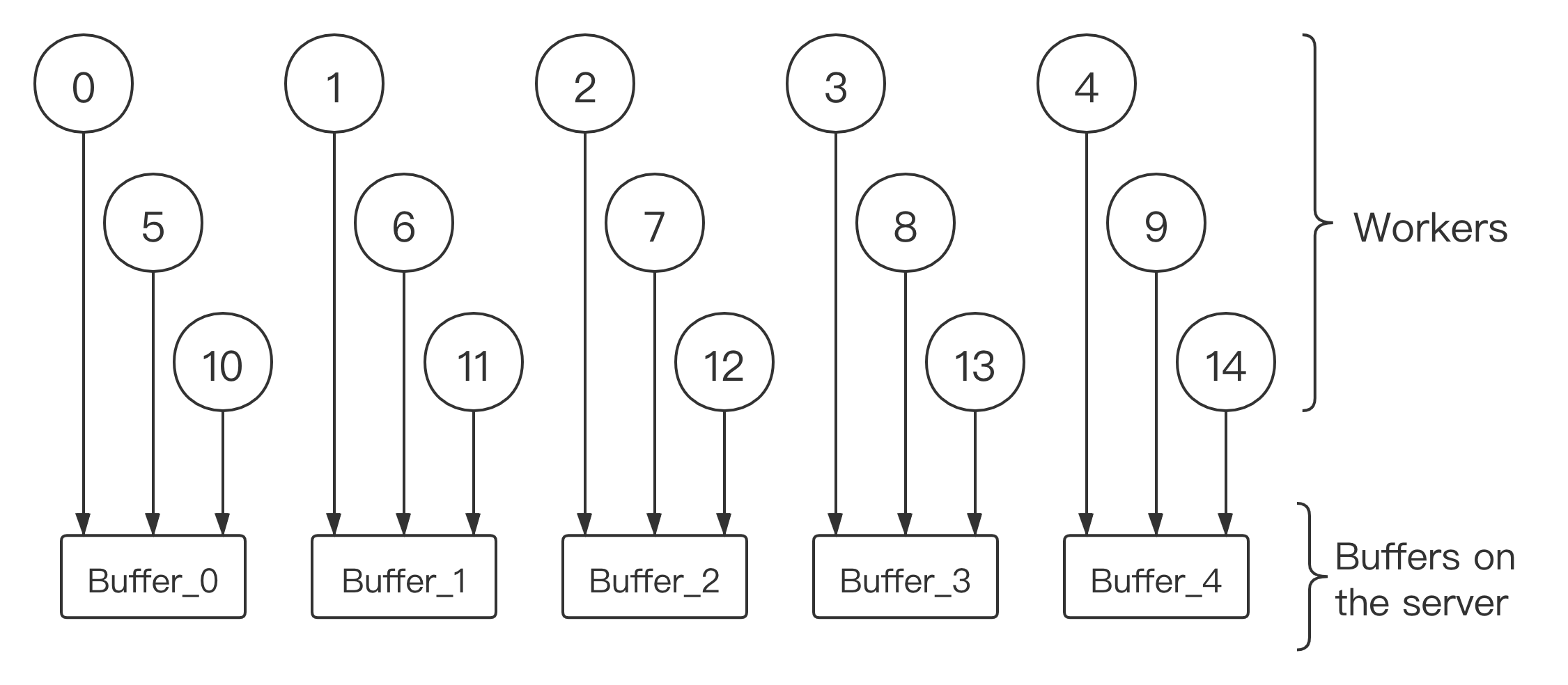
Refer to caption

Figure 1: An example of buffers. Circle represents worker, and the number is worker ID. There are 1515 workers and 55 buffers. The gradient received from worker_ss is stored in buffer_{ss mod 55}.

3.1 Buffer

In BASGD, the mm workers do the same job as that in ASGD, while the updating rule on server is modified. More specifically, there are BB buffers (0<B≤m0<B\leq m) on server. When a gradient 𝐠{\bf g} from worker_ss is received, it will be temporarily stored in buffer bb, where b=s​m​o​d​Bb=s~mod~B, as illustrated in Figure 1. Only when each buffer has stored at least one gradient, a new SGD step will be executed. Please note that no matter whether a SGD step is executed or not, the server will immediately send the latest parameters back to the worker after receiving a gradient. Hence, BASGD introduces no barrier, and is an asynchronous algorithm.

For each buffer bb, more than one gradient may have been received at iteration tt. We will store the average of these gradients (denoted by 𝐡b{\bf h}_{b}) in buffer bb. Assume that there are already (N−1)(N-1) gradients 𝐠1,𝐠2,…,𝐠N−1{\bf g}_{1},{\bf g}_{2},\ldots,{\bf g}_{N-1} which should be stored in buffer bb, and 𝐡b⁡(o​l​d)=1N−1​∑i=1N−1𝐠i.{\bf h}_{b(old)}=\frac{1}{N-1}\sum_{i=1}^{N-1}{\bf g}_{i}. When the NN-th gradient 𝐠N{\bf g}_{N} is received, the new average value is:

𝐡b⁡(n​e​w)=1N​∑i=1N𝐠i=N−1N⋅𝐡b⁡(o​l​d)+1N⋅𝐠N.{\bf h}_{b(new)}=\frac{1}{N}\sum_{i=1}^{N}{\bf g}_{i}=\frac{N-1}{N}\cdot{\bf h}_{b(old)}+\frac{1}{N}\cdot{\bf g}_{N}.

This is the updating rule for each buffer bb when a gradient is received. We use NbtN_{b}^{t} to denote the total number of gradients stored in buffer bb at the tt-th iteration. After the parameter 𝐰{\bf w} is updated, all buffers will be zeroed out at once. With the benefit of buffers, server has access to BB candidate gradients when updating parameter. Thus, a more reliable (robust) gradient can be aggregated from the BB gradients of buffers, if a proper aggregation function A​g​g​r​(⋅)Aggr(\cdot) is chosen.

Please note that from the perspective of workers, BASGD is fully asynchronous, since a worker will immediately receive the latest parameter from the server after sending a gradient to the server, without waiting for other workers. Meanwhile, from the perspective of server, BASGD is semi-asynchronous because the server will not update the model until all buffers are filled. However, it is a necessity to limit the updating frequency in ABL when server has no instances. If the server always updates the model when receiving a gradient, it will be easily foiled when Byzantine workers send gradients much more frequently than others. A similar conclusion has been proved in previous works (Damaskinos et al. 2018).

3.2 Aggregation Function

When a SGD step is ready to be executed, there are BB buffers providing candidate gradients. An aggregation function is needed to get the final gradient for updating. A naive way is to take the mean of all candidate gradients. However, mean value is sensitive to outliers which are common in BL. For designing proper aggregation functions, we first define the qq-Byzantine Robust (qq-BR) condition to quantitatively describe the Byzantine resilience ability of an aggregation function.

Definition 1 (qq-Byzantine Robust).

For an aggregation function A​g​g​r​(⋅)Aggr(\cdot): A​g​g​r​([𝐡1,…𝐶𝐿𝑂𝑆𝐸𝐶𝐿𝑂𝑆𝐸,Aggr([{\bf h}_{1},\ldots, 𝐡B])=𝐆{\bf h}_{B}])={\bf G}, where 𝐆=[G1,…,Gd]T{\bf G}=[G_{1},\ldots,G_{d}]^{T} and 𝐡b=[hb​1,…,hb​d]T,∀b∈[B]{\bf h}_{b}=[h_{b1},\ldots,h_{bd}]^{T},\forall b\in[B], we call A​g​g​r​(⋅)Aggr(\cdot) qq-Byzantine Robust (q∈ℤ,0<q<B/2q\in{\mathbb{Z}},0<q<B/2), if it satisfies the following two properties:

(a) A​g​g​r​([𝐡1+𝐡′,…,𝐡B+𝐡′])=A​g​g​r​([𝐡1,…,𝐡B])+𝐡′,Aggr([{\bf h}_{1}+{\bf h}^{\prime},\ldots,{\bf h}_{B}+{\bf h}^{\prime}])=Aggr([{\bf h}_{1},\ldots,{\bf h}_{B}])+{\bf h}^{\prime},\ ∀𝐡1,…,𝐡B∈ℝd,∀𝐡′∈ℝd;\forall{\bf h}_{1},\ldots,{\bf h}_{B}\in{\mathbb{R}}^{d},\forall{\bf h}^{\prime}\in{\mathbb{R}}^{d};
(b) mins∈𝒮⁡{hs​j}≤Gj≤maxs∈𝒮⁡{hs​j},\min_{s\in{\mathcal{S}}}\{h_{sj}\}\leq G_{j}\leq\max_{s\in{\mathcal{S}}}\{h_{sj}\},\ ∀j∈[d]\forall j\in[d], ∀𝒮⊂[B]\forall{\mathcal{S}}\subset[B] with |𝒮|=B−q.|{\mathcal{S}}|=B-q.

Intuitively, property (a) in Definition 1 says that if all candidate vectors 𝐡i{\bf h}_{i} are added by a same vector 𝐡′{\bf h}^{\prime}, the aggregated gradient will also be added by 𝐡′{\bf h}^{\prime}. Property (b) says that for each coordinate jj, the aggregated value GjG_{j} will be between the (q+1)(q+1)-th smallest value and the (q+1)(q+1)-th largest value among the jj-th coordinates of all candidate vectors. Thus, the gradient aggregated by a qq-BR function is insensitive to at least qq outliers. We can find that qq-BR condition gets stronger when qq increases. Namely, if A​g​g​r​(⋅)Aggr(\cdot) is qq-BR, then for any 0<q′<q0<q^{\prime}<q, A​g​g​r​(⋅)Aggr(\cdot) is also q′q^{\prime}-BR.

Remark 2.

When B>1B>1, mean function is not qq-Byzantine Robust for any q>0q>0. We illustrate this by a one-dimension example: h1,…,hB−1∈[0,1]h_{1},\ldots,h_{B-1}\in[0,1], and hB=10×Bh_{B}=10\times B. Then 1B​∑b=1Bhb≥hBB=10∉[0,1].\frac{1}{B}\sum_{b=1}^{B}h_{b}\geq\frac{h_{B}}{B}=10\not\in[0,1]. Namely, the mean is larger than any of the first B−1B-1 values.

The following two aggregation functions are both qq-BR.

Definition 3 (Coordinate-wise median (Yin et al. 2018)).

For candidate vectors 𝐡1,𝐡2,…{\bf h}_{1},{\bf h}_{2},\ldots, 𝐡B∈ℝd{\bf h}_{B}\in{\mathbb{R}}^{d}, 𝐡b=[hb​1,hb​2,…,hb​d]T{\bf h}_{b}=[h_{b1},h_{b2},\ldots,h_{bd}]^{T}, ∀b=1,2,…,B\forall b=1,2,\ldots,B. Coordinate-wise median is defined as:

M​e​d​([𝐡1,…,𝐡B])=[M​e​d​(h⋅1),…,M​e​d​(h⋅d)]T,Med([{\bf h}_{1},\ldots,{\bf h}_{B}])=[Med(h_{\cdot 1}),\ldots,Med(h_{\cdot d})]^{T},

where M​e​d​(h⋅j)Med(h_{\cdot j}) is the scalar median of the jj-th coordinates, ∀j=1,2,…,d\forall j=1,2,\ldots,d.

Definition 4 (Coordinate-wise qq-trimmed-mean (Yin et al. 2018)).

For any positive interger q<B/2q<B/2 and candidate vectors 𝐡1,𝐡2,…,𝐡B∈ℝd{\bf h}_{1},{\bf h}_{2},\ldots,{\bf h}_{B}\in{\mathbb{R}}^{d}, 𝐡b=[hb​1,hb​2,…,hb​d]T{\bf h}_{b}=[h_{b1},h_{b2},\ldots,h_{bd}]^{T}, ∀b=1,2,…,B\forall b=1,2,\ldots,B. Coordinate-wise qq-trimmed-mean is defined as:

T​r​m​([𝐡1,…,𝐡B])=[T​r​m​(h⋅1),…,T​r​m​(h⋅d)]T,Trm([{\bf h}_{1},\ldots,{\bf h}_{B}])=[Trm(h_{\cdot 1}),\ldots,Trm(h_{\cdot d})]^{T},

where T​r​m​(h⋅j)=1B−2​q​∑b∈ℳjhb​jTrm(h_{\cdot j})=\frac{1}{B-2q}\sum_{b\in{\mathcal{M}}_{j}}h_{bj} is the scalar qq-trimmed-mean. ℳj{\mathcal{M}}_{j} is the subset of {hb​j}b=1B\{h_{bj}\}_{b=1}^{B} obtained by removing the qq largest elements and qq smallest elements.

In the following content, coordinate-wise median and coordinate-wise qq-trimmed-mean are also called median and trmean, respectively. Proposition 5 shows the qq-BR property of these two functions.

Proposition 5.

Coordinate-wise qq-trmean is qq-BR. Coordinate-wise median is ⌊B−12⌋\lfloor\frac{B-1}{2}\rfloor-BR.

Here, ⌊x⌋\lfloor x\rfloor represents the maximum integer that is not larger than xx. According to Proposition 5, both median and trmean are proper choices for aggregation function in BASGD. The proof can be found in Appendix B. Now we define another class of aggregation functions, which is also important for the analysis in Section 4.

Definition 6 (Stable aggregation function).

Aggregation function A​g​g​r​(⋅)Aggr(\cdot) is called stable provided that ∀𝐡1,…,𝐡B\forall{\bf h}_{1},\ldots,{\bf h}_{B}, 𝐡~1,…,𝐡~B∈ℝd\tilde{{\bf h}}_{1},\ldots,\tilde{{\bf h}}_{B}\in{\mathbb{R}}^{d}, letting δ=(∑b=1B‖𝐡b−𝐡~b‖2)12\delta=(\sum_{b=1}^{B}\|{\bf h}_{b}-\tilde{{\bf h}}_{b}\|^{2})^{\frac{1}{2}}, we have:

‖A​g​g​r​(𝐡1,…,𝐡B)−A​g​g​r​(𝐡~1,…,𝐡~B)‖≤δ.\|Aggr({\bf h}_{1},\ldots,{\bf h}_{B})-Aggr(\tilde{{\bf h}}_{1},\ldots,\tilde{{\bf h}}_{B})\|\leq\delta.

If A​g​g​r​(⋅)Aggr(\cdot) is a stable aggregation function, it means that when there is a disturbance with L2L_{2}-norm δ\delta on buffers, the disturbance of aggregated result will not be larger than δ\delta.

Definition 7 (Effective aggregation function).

When there are at most rr Byzantine workers, stable aggregation function A​g​g​r​(⋅)Aggr(\cdot) is called an (A1,A2)(A_{1},A_{2})-effective aggregation function, provided that it satisfies the following two properties for all 𝐰t∈ℝd{\bf w}^{t}\in{\mathbb{R}}^{d} in cases without delay (τkt=0,∀t=0,1,…,T−1\tau_{k}^{t}=0,\ \forall t=0,1,\ldots,T-1):

(a) 𝔼[∇F(𝐰t)T𝐆s​y​nt|𝐰t]≥∥∇F(𝐰t)∥2−A1{\mathbb{E}}[\nabla F({\bf w}^{t})^{T}{\bf G}_{syn}^{t}~|~{\bf w}^{t}]\geq\|\nabla F({\bf w}^{t})\|^{2}-A_{1};
(b) 𝔼⁡[‖𝐆s​y​nt‖2|𝐰t]≤(A2)2{\mathbb{E}}[\|{\bf G}_{syn}^{t}\|^{2}~|~{\bf w}^{t}]\leq(A_{2})^{2};

where A1,A2∈ℝ+A_{1},A_{2}\in{\mathbb{R}}_{+} are two non-negative constants, 𝐆s​y​nt{\bf G}_{syn}^{t} is the aggregated result of A​g​g​r​(⋅)Aggr(\cdot) at the tt-th iteration in cases without delay.

More specifically, 𝐆s​y​nt{\bf G}_{syn}^{t} can be the aggregated gradient or momentum. In the conference version (Yang and Li 2021), 𝐆s​y​nt{\bf G}_{syn}^{t} is the aggregated gradient. We change the statement to make it compatible with BASGDm method, which we will introduce in Section 3.4.

For different aggregation functions, constants A1A_{1} and A2A_{2} may differ. A1A_{1} and A2A_{2} are related to loss function F⁡(⋅)F(\cdot), distribution of instances, buffer number BB, maximum Byzantine worker number rr. Inequalities (a) and (b) in Definition 7 are two important properties in convergence proof of synchronous Byzantine learning methods. As revealed in (Yang et al. 2020), there are many existing aggregation rules for Byzantine learning. We find that most of them satisfy Definition 7. For example, Krum, median, and trimmed-mean have already been proved to satisfy these two properties (Blanchard et al. 2017; Yin et al. 2018). SignSGD (Bernstein et al. 2019) can be seen as a combination of 1-bit quantization and median aggregation, while median satisfies the properties in Definition 7.

Compared to Definition 1, Definition 7 can be used to obtain a tighter bound with respect to A1A_{1} and A2A_{2}. However, it usually requires more effort to check the two properties in Definition 7 than those in Definition 1.

Please note that too large BB could lower the updating frequency and damage the performance, while too small BB may harm the Byzantine resilience. Thus, a moderate BB is usually preferred. In some practical applications, we could estimate the maximum number of Byzantine workers rr, and set BB to make the aggregation function resilient to up to rr Byzantine workers. In particular, BB is suggested to be (2​r+1)(2r+1) for median, since median is ⌊B−12⌋\lfloor\frac{B-1}{2}\rfloor-BR.

Refer to caption

Figure 2: An example of buffer reassignment. White circle represents active worker, and grey circle represents unresponsive worker. Before reassignment, buffer_00 is a straggler. After reassignment, there is at least one active worker corresponding to each buffer.

3.3 Mapping Table

At each iteration of BASGD, buffer_bb needs at least one gradient for aggregation. In the worst case, all the workers corresponding to buffer_bb may be unresponsive. In this case, buffer_bb will become the straggler, and slow down the whole learning process. To deal with this problem, we introduce the mapping table for buffer reassignment technique.

We call a worker active worker if it has responsed at the current iteration. If SGD step has not been excuted for Δ\Delta seconds, the server immediately zeroes out stored gradients in all buffers, equally reassigns active workers to each buffer, and then continues the learning procedure. Hyper-parameter Δ\Delta is called reassignment interval. Figure 2 illustrates an example of reassignment. The grey circles represents unresponsive workers. After reassignment, there are at least one active worker corresponding to each buffer.

Specifically, we introduce a mapping table {βs}s=0m−1\{\beta_{s}\}_{s=0}^{m-1} for buffer reassignment. Initially, βs=s\beta_{s}=s (∀s=0,1,…,m−1)(\forall s=0,1,\ldots,m-1). When reassigning buffers, the server only needs to modify the mapping table {βs}s=0m−1\{\beta_{s}\}_{s=0}^{m-1}, and then stores worker_ss’s gradients in buffer_{βs\beta_{s} mod BB}, instead of buffer_{ss mod BB} any more. Please note that the server only needs to modify the mapping table for buffer reassignment, and there is no need to notify workers.

Besides, a timer is used on the server for indicating when to reassign buffers. The timer is started at the beginning of BASGD, and is restarted immediately after each SGD step or buffer reassignment. When the timer exceeds Δ\Delta seconds, buffers will be zeroed out, and reassignment executed. Hyper-parameter Δ\Delta should be set properly. If Δ\Delta is too small, buffers will be zeroed out too frequently, which may slow down the learning process. If Δ\Delta is too large, straggler buffers could not be eliminated in time.

3.4 Buffered Asynchronous SGD with Momentum

As previous works have revealed, history information can greatly help to resist Byzantine attacks (El-Mhamdi et al. 2020; Allen-Zhu et al. 2020; Karimireddy et al. 2021). Therefore, we introduce momentum into BASGD, and obtain the method buffered asynchronous SGD with momentum (BASGDm). In BASGDm, the algorithm of server is exactly the same as that in BASGD. The only difference is that each worker maintains a local momentum, and sends local momentums to server instead of gradients. The detail of BASGDm is illustrated in Algorithm 2. With the benefit of momentum, BASGDm can achieve stronger Byzantine resilience. In particular, BASGDm can resist both non-omniscient and omniscient attacks, as we will show in Section 5.

Algorithm 2 Buffered Asynchronous SGD with Momentum (BASGDm)
 Server:
 Input: learning rate η\eta, momentum hyper-parameter μ⁡(0≤μ<1)\mu\ (0\leq\mu<1),   reassignment interval Δ\Delta, buffer number BB, aggregation function: A​g​g​r​(⋅)Aggr(\cdot);
 Initialization: initial parameter 𝐰0{\bf w}^{0}, learning rate η\eta;
 Set buffer: 𝐡b←𝟎{\bf h}_{b}\leftarrow{\bf 0}, Nbt←0N_{b}^{t}\leftarrow 0;
 Initialize mapping table βs←s\beta_{s}\leftarrow s (s=0,1,…,m−1)(s=0,1,\ldots,m-1);
 Send initial 𝐰0{\bf w}^{0} to all workers;
 Set t←0t\leftarrow 0, and start the timer;
 repeat
  Wait until receiving 𝐮{\bf u} from some worker_ss;
  Choose buffer: b←βs​m​o​d​Bb\leftarrow\beta_{s}~mod~B;
  Let Nbt←Nbt+1N_{b}^{t}\leftarrow N_{b}^{t}+1, and 𝐡b←(Nbt−1)​𝐡b+𝐮Nbt{\bf h}_{b}\leftarrow\frac{(N_{b}^{t}-1){\bf h}_{b}+{\bf u}}{N_{b}^{t}};
  if Nbt>0N_{b}^{t}>0 for each b∈[B]b\in[B] then
   Aggregate: 𝐆t=A​g​g​r​([𝐡1,…,𝐡B]){\bf G}^{t}=Aggr([{\bf h}_{1},\ldots,{\bf h}_{B}]);
   Execute SGD step: 𝐰t+1←𝐰t−η⋅𝐆t{\bf w}^{t+1}\leftarrow{\bf w}^{t}-\eta\cdot{\bf G}^{t};
   Zero out buffers: 𝐡b←𝟎{\bf h}_{b}\leftarrow{\bf 0}, Nbt←0N_{b}^{t}\leftarrow 0 (b=1,…,B)(b=1,\ldots,B);
   Set t←t+1t\leftarrow t+1, and restart the timer;
  end if
  if the timer has exceeded Δ\Delta seconds then
   Zero out buffers: 𝐡b←𝟎{\bf h}_{b}\leftarrow{\bf 0}, Nbt←0N_{b}^{t}\leftarrow 0 (b=1,…,B)(b=1,\ldots,B);
   Modify the mapping table {βs}s=0m−1\{\beta_{s}\}_{s=0}^{m-1} for buffer reassignment, and restart the timer;
  end if
  Send back the latest parameters back to worker_ss, no matter whether a SGD step is executed or not.
 until stop criterion is satisfied
 Notify all workers to stop;
 Worker_kk:   (k=0,1,…,m−1)(k=0,1,...,m-1)
 Initialization: initial momentum 𝐮←𝟎{\bf u}\leftarrow{\bf 0};
 repeat
  Wait until receiving the latest parameter 𝐰{\bf w} from server;
  Randomly sample an index ii from 𝒟k{\mathcal{D}}_{k};
  Compute stochastic gradient ∇f​(𝐰,zi)\nabla f({\bf w};z_{i});
  Update local momentum 𝐮←μ⋅𝐮+(1−μ)⋅∇f​(𝐰,zi){\bf u}\leftarrow\mu\cdot{\bf u}+(1-\mu)\cdot\nabla f({\bf w};z_{i});
  Send 𝐮{\bf u} to server;
 until receive server’s notification to stop

4 Convergence

In this section, we theoretically prove the convergence and resilience of BASGD and BASGDm against failure or attack. We will introduce three main theorems in this section. The first two theorems are for BASGD. One presents a relatively loose but general bound for all qq-BR aggregation functions, while the other one presents a relatively tight bound for each distinct (A1,A2)(A_{1},A_{2})-effective aggregation function. Since the definition of (A1,A2)(A_{1},A_{2})-effective aggregation function is usually more difficult to verify than qq-BR property, the general bound is also useful.

Similar to the second theorem, the last one is for BASGDm with (A1,A2)(A_{1},A_{2})-effective aggregation function. Here we only present the results. Proof details are in Appendix B. We first make the following assumptions, which have been widely used in stochastic optimization.

Assumption 1 (Lower bound).

Global loss function F⁡(𝐰)F({\bf w}) is bounded below: ∃F∗∈ℝ,F⁡(𝐰)≥F∗,∀𝐰∈ℝd\exists F^{*}\in{\mathbb{R}},F({\bf w})\geq F^{*},\forall{\bf w}\in{\mathbb{R}}^{d}.

Assumption 2 (Bounded bias).

For any loyal worker, it can use locally stored training instances to estimate global gradient with bounded bias κ\kappa: ‖𝔼⁡[∇f​(𝐰,zi)]−∇F​(𝐰)‖≤κ,∀𝐰∈ℝd.\|{\mathbb{E}}[\nabla f({\bf w};z_{i})]-\nabla F({\bf w})\|\leq\kappa,~\forall{\bf w}\in{\mathbb{R}}^{d}.

Assumption 3 (Bounded gradient).

∇F​(𝐰)\nabla F({\bf w}) is bounded: ‖∇F​(𝐰)‖≤D,∀𝐰∈ℝd\|\nabla F({\bf w})\|\leq D,\ \forall{\bf w}\in{\mathbb{R}}^{d}.

Assumption 4 (Bounded variance).

𝔼⁡[‖∇f​(𝐰,zi)−𝔼⁡[∇f​(𝐰,zi)|𝐰]‖2|𝐰]≤σ2,∀𝐰∈ℝd{\mathbb{E}}[||\nabla f({\bf w};z_{i})-{\mathbb{E}}[\nabla f({\bf w};z_{i})|{\bf w}]||^{2}~|~{\bf w}]\leq\sigma^{2},\ \forall{\bf w}\in{\mathbb{R}}^{d}.

Assumption 5 (LL-smoothness).

Global loss function F⁡(𝐰)F({\bf w}) is differentiable and LL-smooth: ‖∇F​(𝐰)−∇F​(𝐰′)‖≤L​‖𝐰−𝐰′‖,∀𝐰,𝐰′∈ℝd.||\nabla F({\bf w})-\nabla F({\bf w}^{\prime})||\leq L||{\bf w}-{\bf w}^{\prime}||,~\forall{\bf w},{\bf w}^{\prime}\in{\mathbb{R}}^{d}.

Let N(t)N^{(t)} be the (q+1)(q+1)-th smallest value in {Nbt}b∈[B]\{N_{b}^{t}\}_{b\in[B]}, where NbtN_{b}^{t} is the number of gradients stored in buffer bb at the tt-th iteration. We define the constant

ΛB,q,r=(B−r)​B−r+1(B−q−1)​(q−r+1),\Lambda_{B,q,r}=\frac{(B-r)\sqrt{B-r+1}}{\sqrt{(B-q-1)(q-r+1)}},

which will appear in Lemma 8 and Lemma 9.

Lemma 8.

If A​g​g​r​(⋅)Aggr(\cdot) is qq-BR, and there are at most rr Byzantine workers (r≤q)(r\leq q), we have:

𝔼⁡[‖𝐆t‖2|𝐰t]≤ΛB,q,r​d⋅(D2+σ2/N(t)).{\mathbb{E}}[||{\bf G}^{t}||^{2}~|~{\bf w}^{t}]\leq\Lambda_{B,q,r}d\cdot(D^{2}+\sigma^{2}/N^{(t)}).
Lemma 9.

If A​g​g​r​(⋅)Aggr(\cdot) is qq-BR, and the total number of heavily delayed workers and Byzantine workers is not larger than r⁡(r≤q)r~(r\leq q), we have:

‖𝔼⁡[𝐆t−∇F​(𝐰t)|𝐰t]‖≤ΛB,q,r​d​(τm​a​x​L⋅[ΛB,q,r​d​(D2+σ2/N(t))]12+σ+κ).\displaystyle||{\mathbb{E}}[{\bf G}^{t}-\nabla F({\bf w}^{t})~|~{\bf w}^{t}]||\leq\Lambda_{B,q,r}d(\tau_{max}L\cdot[\Lambda_{B,q,r}d(D^{2}+\sigma^{2}/N^{(t)})]^{\frac{1}{2}}+\sigma+\kappa).
Theorem 10.

Let D~=1T​∑t=0T−1(D2+σ2/N(t))12\tilde{D}=\frac{1}{T}\sum_{t=0}^{T-1}(D^{2}+\sigma^{2}/N^{(t)})^{\frac{1}{2}}. If A​g​g​r​(⋅)Aggr(\cdot) is qq-BR, B=O⁡(r)B=O(r), and the total number of heavily delayed workers and Byzantine workers is not larger than r⁡(r≤q)r~(r\leq q), with learning rate η=O⁡(1L​T)\eta=O(\frac{1}{L\sqrt{T}}), we have:

∑t=0T−1𝔼⁡[‖∇F​(𝐰t)‖2]T≤O⁡(L⁡[F⁡(𝐰0)−F∗]T12)+O⁡(r​d​D~T12​(q−r+1)12)\displaystyle\frac{\sum_{t=0}^{T-1}{\mathbb{E}}[||\nabla F({\bf w}^{t})||^{2}]}{T}\leq O\left(\frac{L[F({\bf w}^{0})-F^{*}]}{T^{\frac{1}{2}}}\right)+O\left(\frac{rd\tilde{D}}{T^{\frac{1}{2}}(q-r+1)^{\frac{1}{2}}}\right)
+O⁡(r​D​d​σ(q−r+1)12)+O⁡(r​D​d​κ(q−r+1)12)+O⁡(r32​L​D​D~​d32​τm​a​x(q−r+1)34).\displaystyle\qquad\qquad\qquad+O\left(\frac{rDd\sigma}{(q-r+1)^{\frac{1}{2}}}\right)+O\left(\frac{rDd\kappa}{(q-r+1)^{\frac{1}{2}}}\right)+O\left(\frac{r^{\frac{3}{2}}LD\tilde{D}d^{\frac{3}{2}}\tau_{max}}{(q-r+1)^{\frac{3}{4}}}\right).

Please note that the convergence rate of vanilla ASGD is O⁡(1/T12)O(1/T^{\frac{1}{2}}). Hence, Theorem 10 indicates that BASGD has a theoretical convergence rate as fast as vanilla ASGD, with an extra constant variance. The term O⁡(r​D​d​σ/(q−r+1)12)O(rDd\sigma/(q-r+1)^{\frac{1}{2}}) is caused by the aggregation function, which can be deemed as a sacrifice for Byzantine resilience. The term O⁡(r​D​d​κ/(q−r+1)12)O(rDd\kappa/(q-r+1)^{\frac{1}{2}}) is caused by the differences of training instances among different workers. In independent and identically distributed (i.i.d.) cases, κ=0\kappa=0 and the term vanishes. The term O⁡(r32​L​D​D~​d32​τm​a​x/(q−r+1)34)O(r^{\frac{3}{2}}LD\tilde{D}d^{\frac{3}{2}}\tau_{max}/(q-r+1)^{\frac{3}{4}}) is caused by the delay, and related to parameter τm​a​x\tau_{max}. The term is also related to the buffer size. When NbtN_{b}^{t} increases, N(t)N^{(t)} may increase, and thus D~\tilde{D} will decrease. Namely, larger buffer size will result in smaller D~\tilde{D}. Besides, the factor (q−r+1)−12(q-r+1)^{-\frac{1}{2}} or (q−r+1)−34(q-r+1)^{-\frac{3}{4}} decreases as qq increases, and increases as rr increases.

Although general, the bound presented in Theorem 10 is relatively loose in high-dimensional cases, since dd appears in all the three extra terms. To obtain a tighter bound, we introduce Theorem 11 for BASGD with (A1,A2)(A_{1},A_{2})-effective aggregation function (Definition 7).

Theorem 11.

In BASGD, if the total number of heavily delayed workers and Byzantine workers is not larger than rr, B=O⁡(r)B=O(r), and A​g​g​r​(⋅)Aggr(\cdot) is an (A1,A2)(A_{1},A_{2})-effective aggregation function. With learning rate η=O⁡(1L​T)\eta=O(\frac{1}{\sqrt{LT}}) satisfying that 2​η2​L2​τm​a​x2​(B−r)<12\eta^{2}L^{2}\tau_{max}^{2}(B-r)<1, in general asynchronous cases we have:

∑t=0T−1𝔼⁡[‖∇F​(𝐰t)‖2]T≤O⁡(L12​[F⁡(𝐰0)−F∗]T12)+O\displaystyle\frac{\sum_{t=0}^{T-1}{\mathbb{E}}[\|\nabla F({\bf w}^{t})\|^{2}]}{T}\leq O\left(\frac{L^{\frac{1}{2}}[F({\bf w}^{0})-F^{*}]}{T^{\frac{1}{2}}}\right)+O (L12​τm​a​x​D​A2​r12T12)+O⁡(L12​(A2)2T12)\displaystyle\left(\frac{L^{\frac{1}{2}}\tau_{max}DA_{2}r^{\frac{1}{2}}}{T^{\frac{1}{2}}}\right)+O\left(\frac{L^{\frac{1}{2}}(A_{2})^{2}}{T^{\frac{1}{2}}}\right)
+O⁡(L52​(A2)2​τm​a​x2​rT32)+A1.\displaystyle+O\left(\frac{L^{\frac{5}{2}}(A_{2})^{2}\tau_{max}^{2}r}{T^{\frac{3}{2}}}\right)+A_{1}.

Theorem 11 indicates that if A​g​g​r​(⋅)Aggr(\cdot) makes a synchronous BL method converge (i.e., satisfies Definition 7), BASGD converges when using A​g​g​r​(⋅)Aggr(\cdot) as aggregation function. Hence, BASGD can also be seen as a technique of asynchronization. That is to say, new asynchronous methods can be obtained from synchronous ones when using BASGD. The extra constant term A1A_{1} is caused by gradient bias. When there is no Byzantine workers (r=0r=0), and instances are i.i.d. across workers, letting B=1B=1 and A​g​g​r​(𝐡1,…,𝐡B)=A​g​g​r​(𝐡1)=𝐡1Aggr({\bf h}_{1},\ldots,{\bf h}_{B})=Aggr({\bf h}_{1})={\bf h}_{1}, BASGD degenerates to vanilla ASGD. In this case, there is no gradient bias (A1=0A_{1}=0), and BASGD has a convergence rate of O⁡(1/T12)O(1/T^{\frac{1}{2}}), which is the same as that of vanilla ASGD (Liu and Zhang 2021).

Meanwhile, it remains uncertain whether the dependence to the staleness parameter τm​a​x\tau_{max} is tight enough. Theorem 11 illustrates that BASGD has a convergence rate of O⁡(τm​a​x/T12)O(\tau_{max}/T^{\frac{1}{2}}), while the convergence rate of vanilla ASGD can reach O⁡(τm​a​x/T)O(\tau_{max}/T). To the best of our knowledge, there exist few works revealing the tightness of τm​a​x\tau_{max} in asynchronous BL, and we will leave this for future work.

Similarly, we have the following theoretical results for BASGDm.

Theorem 12.

In BASGDm, if the total number of heavily delayed workers and Byzantine workers is not larger than rr, B=O⁡(r)B=O(r), and A​g​g​r​(⋅)Aggr(\cdot) is an (A1,A2)(A_{1},A_{2})-effective aggregation function. With learning rate η=O⁡(1L​T)\eta=O(\frac{1}{\sqrt{LT}}) satisfying that 2​η2​L2​τm​a​x2​(1−μ)2​(B−r)<12\eta^{2}L^{2}\tau_{max}^{2}(1-\mu)^{2}(B-r)<1, in general asynchronous cases we have:

∑t=0T−1𝔼⁡[‖∇F​(𝐰t)‖2]T≤\displaystyle\frac{\sum_{t=0}^{T-1}{\mathbb{E}}[\|\nabla F({\bf w}^{t})\|^{2}]}{T}\leq O⁡(L12​[F⁡(𝐰0)−F∗]T12)+O⁡(L12​τm​a​x​D​A2​r12​(1−μ)T12)\displaystyle O\left(\frac{L^{\frac{1}{2}}[F({\bf w}^{0})-F^{*}]}{T^{\frac{1}{2}}}\right)+O\left(\frac{L^{\frac{1}{2}}\tau_{max}DA_{2}r^{\frac{1}{2}}(1-\mu)}{T^{\frac{1}{2}}}\right)
+O⁡(L12​(A2)2T12)+O⁡(L52​(A2)2​τm​a​x2​r​(1−μ)2T32)+A1.\displaystyle+O\left(\frac{L^{\frac{1}{2}}(A_{2})^{2}}{T^{\frac{1}{2}}}\right)+O\left(\frac{L^{\frac{5}{2}}(A_{2})^{2}\tau_{max}^{2}r(1-\mu)^{2}}{T^{\frac{3}{2}}}\right)+A_{1}.

Please note that when momentum hyper-parameter μ=0\mu=0, BASGDm degenerates to BASGD. In this case, 1−μ=11-\mu=1, and Theorem 12 is exactly the same as Theorem 11. From this perspective, Theorem 12 can be deemed as a more general version of Theorem 11. Besides, we would also like to point out that the factor (1−μ)(1-\mu) in Theorem 12 does not mean that larger μ\mu will lead to tighter upper bound, since constants A1A_{1} and A2A_{2} are dependent on momentum hyper-parameter μ\mu. In fact, the influence of momentum hyper-parameter is a complex problem, which has been studied for decades (Qian 1999). Since it is not the focus of this work, we are not going to further discuss this problem here.

In general cases, Theorem 11 and Theorem 12 guarantee BASGD and BASGDm to find a point such that the squared L2L_{2}-norm of its gradient is not larger than A1A_{1} in expectation, respectively. Please note that Assumption 3 already guarantees that gradient’s squared L2L_{2}-norm is not larger than D2D^{2}. We introduce Proposition 13 to show that A1A_{1} is guaranteed to be smaller than D2D^{2} under a mild condition.

Proposition 13.

Assume A​g​g​r​(⋅)Aggr(\cdot) is an (A1,A2)(A_{1},A_{2})-effective aggregation function, and 𝐆s​y​nt{\bf G}_{syn}^{t} is aggregated by A​g​g​r​(⋅)Aggr(\cdot) in synchronous setting. If 𝔼⁡[‖𝐆s​y​nt−∇F​(𝐰t)‖|𝐰t]≤D,{\mathbb{E}}[\|{\bf G}_{syn}^{t}-\nabla F({\bf w}^{t})\|~|~{\bf w}^{t}]\leq D, ∀𝐰t∈ℝd\forall{\bf w}^{t}\in{\mathbb{R}}^{d}, we have A1≤D2A_{1}\leq D^{2}.

𝐆s​y​nt{\bf G}_{syn}^{t} is the aggregated result of A​g​g​r​(⋅)Aggr(\cdot), and is a robust estimator of ∇F​(𝐰t)\nabla F({\bf w}^{t}) used for updating. Since ‖∇F​(𝐰t)‖≤D\|\nabla F({\bf w}^{t})\|\leq D, ∇F​(𝐰t)\nabla F({\bf w}^{t}) locates in a ball with radius DD. 𝔼⁡[‖𝐆s​y​nt−∇F​(𝐰t)‖|𝐰t]≤D{\mathbb{E}}[\|{\bf G}_{syn}^{t}-\nabla F({\bf w}^{t})\|~|~{\bf w}^{t}]\leq D means that the bias of 𝐆s​y​nt{\bf G}_{syn}^{t} is not larger than the radius DD, which is a mild condition for A​g​g​r​(⋅)Aggr(\cdot).

5 Experiment

In this section, we empirically evaluate the performance of BASGD (BASGDm) and baselines in both image classification (IC) and natural language processing (NLP) applications. Our experiments are conducted on a distributed platform with dockers. Each docker is bound to an NVIDIA Tesla V100 (32G) GPU. We choose 3030 dockers as workers and an extra docker as server11 1 In the conference version (Yang and Li 2021), we set 88 workers in NLP experiment. To make the settings more consistent with that of IC experiment, we also set worker number to 3030 for NLP experiment in this journal version.. All algorithms are implemented with PyTorch 1.3.

5.1 Experimental Setting

Because BASGD (BASGDm) is ABL methods, SBL methods cannot be directly compared with BASGD (BASGDm). The ABL method Zeno++ either cannot be directly compared with BASGD (BASGDm), because Zeno++ needs to store some instances on server. The number of instances stored on server will highly affect the performance of Zeno++ (Xie et al. 2020b). Hence, we compare BASGD (BASGDm) with ASGD (ASGDm) and Kardam in our experiments. We set dampening function Λ⁡(τ)=11+τ\Lambda(\tau)=\frac{1}{1+\tau} for Kardam as suggested in (Damaskinos et al. 2018), and set momentum hyper-parameter μ=0.9\mu=0.9 for BASGDm and ASGDm in each experiment.

Byzantine attacks. We will compare BASGD (BASGDm) with baselines under the following different attack settings.

  • •

    No attack: In this setting, each worker will strictly follow the method, compute and send the gradient (or momentum) without error.

  • •

    Random disturbance attack (RD-attack): Byzantine workers with RD-attack will replace the true gradient 𝐠{\bf g} with 𝐠~R​D=𝐠+𝐠r​n​d\tilde{{\bf g}}_{RD}={\bf g}+{\bf g}_{rnd}, where 𝐠r​n​d{\bf g}_{rnd} is a random vector sampled from normal distribution 𝒩⁡(𝟎,‖σa​t​k​𝐠‖2⋅𝐈){\mathcal{N}}({\bf 0},\|\sigma_{atk}{\bf g}\|^{2}\cdot{\bf I}). Here, σa​t​k\sigma_{atk} is a parameter and 𝐈{\bf I} is an identity matrix. We set σa​t​k=0.2\sigma_{atk}=0.2 in our experiments. RD-attack can be seen as an accidental failure with expectation 𝟎{\bf 0}.

  • •

    Negative gradient attack (NG-attack): Byzantine workers with NG-attack will replace the true gradient 𝐠{\bf g} with 𝐠~N​G=−ka​t​k⋅𝐠\tilde{{\bf g}}_{NG}=-k_{atk}\cdot{\bf g}, where ka​t​k∈ℝ+k_{atk}\in{\mathbb{R}}_{+} is a parameter. We set ka​t​k=10k_{atk}=10 in our experiments. NG-attack is a typical kind of malicious attack. In some previous works, this type of attack is also called bit-flipping attack (Xie et al. 2020b; Karimireddy et al. 2021).

  • •

    ‘Fall of Empires’ (FoE) attack (Xie et al. 2020a): Byzantine workers with FoE attack will replace the gradient 𝐠{\bf g} with 𝐠~F​o​E=−ϵ|ℒ|∑i∈ℒ𝐠i\tilde{{\bf g}}_{FoE}=-\frac{\epsilon}{|{\mathcal{L}}|}\sum_{i\in{\mathcal{L}}}{\bf g}_{i}, where ℒ{\mathcal{L}} is the index set of loyal workers and 𝐠i{\bf g}_{i} is the gradient computed by the ii-th worker at the same iteration. We set hyper-parameter ϵ=6\epsilon=6 for FoE attack in the experiments of this work. FoE is a type of omniscient attack originally proposed in synchronous settings, which require the gradients computed by loyal workers at the same iteration as omniscient knowledge. Thus, FoE cannot be directly adopted in asynchronous settings. To deal with this problem, we use the last sent gradient (or momentum) from each loyal worker as the omniscient knowledge for FoE.

  • •

    ‘A Little is Enough’ (ALIE) attack (Baruch et al. 2019): Byzantine workers with ALIE attack will replace the gradient 𝐠{\bf g} with 𝐠~A​L​I​E\tilde{{\bf g}}_{ALIE}, where (𝐠~A​L​I​E)j=m​e​a​nj−zm​a​x⋅s​t​dj(\tilde{{\bf g}}_{ALIE})_{j}={mean}_{j}-z^{max}\cdot{std}_{j}. The sub-index (⋅)j(\cdot)_{j} denotes the jj-th coordinate of the vector. The scalars m​e​a​nj{mean}_{j} and s​t​dj{std}_{j} are the mean and standard error of the jj-th coordinate of loyal workers’ gradients at the same iteration, respectively. zm​a​x=Φ−1​(m−⌊m/2+1⌋m−r)z^{max}=\Phi^{-1}(\frac{m-\lfloor m/2+1\rfloor}{m-r}), where Φ−1​(⋅)\Phi^{-1}(\cdot) is the inverse of the standard normal cumulative distribution function, mm is the number of workers, and rr is the number of Byzantine workers. ALIE is also a type of omniscient attack originally proposed in synchronous settings. Similarly, to make it compatible with asynchronous settings, we use the last sent gradient (or momentum) from each loyal worker as the omniscient knowledge for ALIE.

In real world applications, it is usually hard to adopt the two types of omniscient attacks (FoE and ALIE) due to the lack of omniscient knowledge. However, we still compare the performance of different methods under these two attacks to test resilience ability.

Aggregation rules. In the experiments, BASGDm is tested with each of the following aggregation rules.

  • •

    Coordinate-wise qq-trimmed-mean (trmean): Please refer to Definition 4.

  • •

    Coordinate-wise median (median): Please refer to Definition 3. Since median can be deemed as a special case of trmean, we only report the results of BASGD (BASGDm) with median in the no attack case22 2 In the conference version (Yang and Li 2021), we report the results of BASGD with median in all cases. In this journal version, we test BASGD (BASGDm) with two more aggregation rules (geometric median and centered clipping). Due to limited space in each single figure, we do not report the results of BASGD (BASGDm) with median for better readability in this journal version. The performance of median is similar to that of other aggregation rules..

  • •

    Geometric median (geoMed) (Chen et al. 2017): The geometric median of BB vectors 𝐡1,…,𝐡B∈ℝd{\bf h}_{1},\ldots,{\bf h}_{B}\in{\mathbb{R}}^{d} is defined as:

    geoMed​([𝐡1,…,𝐡B])=arg⁡min𝐡∈ℝd⁡{∑b=1B‖𝐡−𝐡b‖2}.\text{geoMed}([{\bf h}_{1},\ldots,{\bf h}_{B}])=\mathop{\arg\min}_{{\bf h}\in{\mathbb{R}}^{d}}\left\{\sum_{b=1}^{B}\|{\bf h}-{\bf h}_{b}\|_{2}\right\}. (2)

    The optimization problem defined in the right-hand side of (2) has a unique solution when vectors {𝐡1,…,𝐡B}\{{\bf h}_{1},\ldots,{\bf h}_{B}\} do not lie in a line. However, geoMed usually does not have a closed-form solution. We use Weiszfeld’s algorithm (Pillutla et al. 2019) to compute it and set the iteration number in Weiszfeld’s algorithm to be 55.

  • •

    Centered clipping (CC) (Karimireddy et al. 2021): The CC aggregation result of vectors {𝐡1,…,𝐡B}\{{\bf h}_{1},\ldots,{\bf h}_{B}\} is given by the following iteration formula:

    𝐡l+1=𝐡l+1B​∑b=1B(𝐡b−𝐡l)​min⁡(1,R‖𝐡b−𝐡l‖2).{\bf h}^{l+1}={\bf h}^{l}+\frac{1}{B}\sum_{b=1}^{B}({\bf h}_{b}-{\bf h}^{l})\min\left(1,\frac{R}{\|{\bf h}_{b}-{\bf h}^{l}\|_{2}}\right). (3)

    We set initial point 𝐡0{\bf h}^{0} to be the last aggregation result for quicker convergence as suggested in (Karimireddy et al. 2021). The iteration number is set to be 55 in IC task and 5050 in NLP task. Clipping size RR is set to be 0.50.5.

In addition, to simulate an unstable network environment where asynchronous methods are usually preferred, each worker is manually set to have a delay, which is kd​e​lk_{del} times the computing time. Training set is randomly and equally distributed to different workers. We use the average top-11 test accuracy (in IC) or average perplexity (in NLP) on all workers w.r.t. epochs as final metrics. Average training loss w.r.t. epochs in IC experiment can be found in Appendix C, which is consistent with the average top-11 test accuracy results presented in this section. For BASGD (BASGDm), reassignment interval is set to be 11 second in the IC experiment and 55 seconds in the NLP experiment.

5.2 Image Classification Experiment

(a) BASGD with median
(b) BASGD with trmean
(c) BASGD with geoMed
(d) BASGD with CC
Figure 3: Average top-11 test accuracy w.r.t. epochs of methods BASGD, ASGD, and Kardam when there are no Byzantine workers.
(a) BASGDm with median
(b) BASGDm with trmean
(c) BASGDm with geoMed
(d) BASGDm with CC
Figure 4: Average top-11 test accuracy w.r.t. epochs of methods BASGDm, ASGDm, and Kardam when there are no Byzantine workers.

In this part, we will empirically compare the performance of BASGD (BASGDm) and existing asynchronous methods ASGD and Kardam in image classification tasks.

In the experiment, algorithms are evaluated on CIFAR-10 (Krizhevsky et al. 2009) with deep learning model ResNet-20 (He et al. 2016). Cross-entropy is used as the loss function. kd​e​lk_{del} is randomly sampled from truncated standard normal distribution within [0,+∞)[0,+\infty). As suggested in (He et al. 2016), learning rate η\eta is set to 0.10.1 initially for each algorithm, and multiplied by 0.1 at the 8080-th epoch and the 120120-th epoch respectively. The weight decay is set to 10−410^{-4}. We run each algorithm for 160160 epochs. Batch size is set to 2525.

Firstly, we compare the performance of different methods when there are no Byzantine workers. Experimental results of BASGD and BASGDm are illustrated in Figure 3 and Figure 4, respectively. The solid line represents that the method does not use momentum while the dotted line represents that the method utilizes local momentum. ASGD (ASGDm) achieves the best performance. BASGD (BASGDm) (B>1B>1) and Kardam have similar convergence rate to ASGD (ASGDm), but both sacrifice a little accuracy. Furthermore, the performance of BASGD (BASGDm) gets worse when the buffer number BB increases, which is consistent with the theoretical results. Please note that ASGD (ASGDm) is a degenerated case of BASGD (BASGDm) when B=1B=1 and A​g​g​r​(𝐡1)=𝐡1Aggr({\bf h}_{1})={\bf h}_{1}. Hence, BASGD (BASGDm) can achieve the same performance as ASGD (ASGDm) when there is no failure or attack. The wall-clock-time of running 160160 epochs is reported in Table 1. The time cost of BASGDm is slightly larger than that of ASGD, while Kardam takes the most time.

Table 1: Wall-clock-time of running 160160 epochs for different methods (in seconds)
Method ASGD BASGDm (B=10B=10) Kardam
w/ trmean w/ geoMed w/ CC γ=2\gamma=2 γ=10\gamma=10
Wall-clock-time 1172.30 1191.01 1287.07 1289.32 1522.05 1535.22
(a) 33 Byzantine workers with RD-attack
(b) 33 Byzantine workers with NG-attack
(c) 66 Byzantine workers with RD-attack
(d) 66 Byzantine workers with NG-attack
Figure 5: Average top-11 test accuracy w.r.t. epochs under non-omniscient attacks. B=10B=10 for BASGD (BASGDm) when there are 33 Byzantine workers and B=15B=15 for BASGD (BASGDm) when there are 66 Byzantine workers.

Then, for each type of attack, we compare the performance of BASGD (BASGDm) and Kardam by conducting two experiments in which there are 33 and 66 Byzantine workers, respectively33 3 In the conference version (Yang and Li 2021), we also report the experimental results of ASGD under attacks. However, due to limit space in figures, we do not report the results of ASGD (ASGDm) in this journal version for better readability since ASGD (ASGDm) is not Byzantine-resilient.. We respectively set 1010 and 1515 buffers for BASGD (BASGDm) in these two experiments. The experimental results of the methods under two types of non-omniscient attacks (RD-attack and NG-attack) are presented in Figure 5. We can find that BASGD (BASGDm) significantly outperform Kardam under these two types of non-omniscient attacks.

Under the less harmful RD-attack, although Kardam still converge, it suffers a significant loss on accuracy. Under NG-attack, Kardam cannot converge even if we have tried different values of assumed Byzantine worker number for Kardam, which is denoted by the hyper-parameter γ\gamma in this paper. Hence, Kardam cannot resist these two types of attacks. On the contrary, BASGD still has a relatively good performance under both types of non-omniscient attacks.

Moreover, we count the ratio of filtered gradients in Kardam, which is shown in Table 2. We can find that in order to filter Byzantine gradients, Kardam also filters approximately equal ratio of loyal gradients. It explains why Kardam performs poorly under the attack.

Table 2: Filtered ratio in Kardam under NG-attack in IC task (33 Byzantine workers)
Term By Frequency Filter By Lipschitz Filter In total
Loyal Grads (γ=3\gamma=3) 10.15%​(31202/307530)10.15\%~(31202/307530) 40.97%​(126000/307530)40.97\%~(126000/307530) 51.12%51.12\%
Byzt Grads (γ=3\gamma=3) 10.77%​(3681/34170)10.77\%~(3681/34170) 40.31%​(13773/34170)40.31\%~(13773/34170) 51.08%51.08\%
Loyal Grads (γ=8\gamma=8) 28.28%​(86957/307530)28.28\%~(86957/307530) 28.26%​(86893/307530)28.26\%~(86893/307530) 56.53%56.53\%
Byzt Grads (γ=8\gamma=8) 28.38%​(9699/34170)28.38\%~(9699/34170) 28.06%​(9588/34170)28.06\%~(9588/34170) 56.44%56.44\%
Loyal Grads (γ=14\gamma=14) 85.13%​(261789/307530)85.13\%~(261789/307530) 3.94%​(12117/307530)3.94\%~(12117/307530) 89.07%89.07\%
Byzt Grads (γ=14\gamma=14) 84.83%​(28985/34170)84.83\%~(28985/34170) 4.26%​(1455/34170)4.26\%~(1455/34170) 89.08%89.08\%
(a) 33 Byzantine workers with FoE attack
(b) 33 Byzantine workers with ALIE attack
(c) 66 Byzantine workers with FoE attack
(d) 66 Byzantine workers with ALIE attack
Figure 6: Average top-11 test accuracy w.r.t. epochs under omniscient attacks. B=10B=10 for BASGD (BASGDm) when there are 33 Byzantine workers and B=15B=15 for BASGD (BASGDm) when there are 66 Byzantine workers.

We also compare the performance of different methods under omniscient attacks (FoE attack and ALIE attack), the results of which are shown in Figure 6. BASGDm can significantly outperform other methods in each case, except for the case of 33 Byzantine workers with ALIE attack. When there are 33 Byzantine workers with ALIE attack, all the methods have a comparable performance to each other. The main reason is that the Byzantine attack is not strong enough in this case. In addition, the performance of BASGDm is considerably better than BASGD. This reveals that using history information (such as momentum) can strengthen the resilience and improve the performance in Byzantine-resilient machine learning, which is consistent with previous works (Allen-Zhu et al. 2020; El-Mhamdi et al. 2020; Karimireddy et al. 2021). Moreover, although the performance of BASGDm with different aggregation rules (trmean, geoMed, and CC) slightly differ, all of them can outperform BASGD and Kardam.

5.3 Natural Language Processing Experiment

(a) Under RD-attack
(b) Under NG-attack
(c) Under FoE attack
(d) Under ALIE attack
Figure 7: Average perplexity w.r.t. epochs (33 Byzantine workers, B=15B=15 for BASGD and BASGDm). In subfigure , the curves representing Kardam do not appear because Kardam diverges in this case and the average perplexity explodes.

In this part, we will empirically compare the methods on natural language processing (NLP) tasks. In our NLP experiment, the methods are evaluated on the WikiText-2 dataset with an LSTM (Hochreiter and Schmidhuber 1997) network. We only use the training set and test set, while the validation set is not used in our experiment. For LSTM, we adopt 22 layers with 100100 units in each layer. Word embedding size is set to 100100, and sequence length is set to 3535. Gradient clipping size is set to 0.250.25. Cross-entropy is used as the loss function. We run each algorithm for 4040 epochs. Initial learning rate η\eta is chosen from {1,2,5,10,20}\{1,2,5,10,20\} and is divided by 44 at the 2121-st epoch and the 3131-st epoch. The best result is adopted as the final one. kd​e​lk_{del} is randomly sampled from a standard exponential distribution. Similarly, each method is tested under RD-attack, NG-attack, FoE attack, and ALIE attack. The average perplexity is reported in Figure 7.

As illustrated in Figure 7(a) and Figure 7(b), under the two types of non-omniscient attacks (RD-attack and NG-attack), BASGD (BASGDm) can outperform Kardam, no matter which of the three aggregation rules is used. Moreover, the curves representing Kardam do not appear in Figure 7(b) because Kardam diverges under NG-attack and the perplexity explodes. We would also like to clarify that the performance of CC can get further improved by tuning the clipping size hyper-parameter more finely in different settings. However, it requires much computing power and is beyond the scope of this work. Therefore, we fix clipping size R=0.5R=0.5, and this can already make BASGDm with CC outperform Kardam. Theoretically, the best performance of CC can not be worse than geoMed since CC is equivalent to geoMed when the clipping size RR is small enough (please see Appendix B.8 for the proof).

As illustrated in Figure 7(c) and Figure 7(d), under FoE attack and ALIE attack, BASGD can outperform Kardam except for the case of using trmean as aggregation rule. BASGD with trmean performs slightly worse than Kardam. A possible reason is that trmean is sensitive to model dimensions. On the contrary, by using momentum, BASGDm with any aggregation rule can always outperform Kardam.

The experimental results in this section have shown that BASGD (BASGDm) can outperform asynchronous Byzantine learning baselines under different settings. Moreover, BASGD (BASGDm) is compatible with various aggregation rules, such as trmean, geoMed, and CC. With the benefit of local momentum, BASGDm gets even stronger Byzantine resilience than BASGD, especially under the omniscient attacks FoE and ALIE.

6 Conclusion

In this paper, we propose a novel method called BASGD and an improved variant of BASGD called BASGDm. To the best of our knowledge, BASGD is the first ABL method that can resist non-omniscient attacks without storing any instances on server. With the benefit of local momentum, BASGDm can resist both non-omniscient and omniscient attacks. Compared with those methods which need to store instances on server, BASGD and BASGDm have a wider scope of application. Both BASGD and BASGDm are compatible with various aggregation rules. Moreover, both BASGD and BASGDm are proved to be convergent and be able to resist failure or attack. Empirical results show that our methods significantly outperform existing ABL baselines when there exists failure or attack on workers.

acknowledgments-disclosure-of-funding.
This work is supported by National Key R&D Program of China (No. 2020YFA0713900), NSFC-NRF Joint Research Project (No. 61861146001) and NSFC Project (No. 61921006).

Appendix A Asynchronous SGD (ASGD)

One popular asynchronous method to solve the problem in (1) under the PS framework is ASGD (Dean et al. 2012), which is presented in Algorithm 3.

Algorithm 3 Asynchronous SGD (ASGD)
 Server:
 Initialization: initial parameter 𝐰0{\bf w}^{0}, learning rate η\eta;
 Send initial 𝐰0{\bf w}^{0} to all workers;
 for t=0t=0 to tm​a​x−1t_{max}-1 do
  Wait until a new gradient 𝐠kt{\bf g}_{k}^{t} is received from arbitrary worker_kk;
  Execute SGD step: 𝐰t+1←𝐰t−η⋅𝐠kt{\bf w}^{t+1}\leftarrow{\bf w}^{t}-\eta\cdot{\bf g}_{k}^{t};
  Send 𝐰t+1{\bf w}^{t+1} back to worker_kk;
 end for
 Notify all workers to stop;
 Worker_kk:   (k=0,1,…,m−1)(k=0,1,...,m-1)
 repeat
  Wait until receiving the latest parameter 𝐰{\bf w} from server;
  Randomly sample an index ii from 𝒟k{\mathcal{D}}_{k};
  Compute ∇f​(𝐰,zi)\nabla f({\bf w};z_{i});
  Send ∇f​(𝐰,zi)\nabla f({\bf w};z_{i}) to server;
 until receive server’s notification to stop

Appendix B Proof Details

B.1 Proof of Proposition 5

Proof.

Firstly, we prove coordinate-wise qq-trimmed-mean is qq-BR. It is not hard to check that trmean satisfies the property (a) in the definition of qq-BR, then we prove that it also satisfies property (b).

Without loss of generality, we assume h1​j,…,hB​jh_{1j},\ldots,h_{Bj} are already in descending order. By definition, T​r​m​(h⋅j)Trm(h_{\cdot j}) is the average value of ℳj{\mathcal{M}}_{j}, which is obtained by removing qq largest values and qq smallest values of {hi​j}i=1B\{h_{ij}\}_{i=1}^{B}. Therefore,

h(q+1)​j=maxx∈ℳj⁡{x}≥T​r​m​(h⋅j)≥minx∈ℳj⁡{x}=h(n−q)​jh_{(q+1)j}=\max_{x\in{\mathcal{M}}_{j}}\{x\}\geq Trm(h_{\cdot j})\geq\min_{x\in{\mathcal{M}}_{j}}\{x\}=h_{(n-q)j}

For any 𝒮⊂[B]{\mathcal{S}}\subset[B] with |𝒮|=B−q|{\mathcal{S}}|=B-q, by Pigeonhole Principle, 𝒮{\mathcal{S}} includes at least one of h1​j,…,h(q+1)​jh_{1j},\ldots,h_{(q+1)j}, and includes at least one of h(n−q)​j,…,hB​jh_{(n-q)j},\ldots,h_{Bj}. Therefore,

maxs∈𝒮⁡{hs​j}≥h(q+1)​j;mins∈𝒮⁡{hs​j}≤h(n−q)​j.\max_{s\in{\mathcal{S}}}\{h_{sj}\}\geq h_{(q+1)j};\qquad\min_{s\in{\mathcal{S}}}\{h_{sj}\}\leq h_{(n-q)j}.

Combining these two inequalities, we have:

maxs∈𝒮⁡{hs​j}≥T​r​m​(h⋅j)≥mins∈𝒮⁡{hs​j}.\max_{s\in{\mathcal{S}}}\{h_{sj}\}\geq Trm(h_{\cdot j})\geq\min_{s\in{\mathcal{S}}}\{h_{sj}\}.

Thus, coordinate-wise qq-trimmed-mean is qq-BR.
By definition, coordinate-wise median can be seen as ⌊B−12⌋\lfloor\frac{B-1}{2}\rfloor-trimmed-mean, and thus is ⌊B−12⌋\lfloor\frac{B-1}{2}\rfloor-BR. ∎

B.2 Proof of Lemma 8

To begin with, we will introduce a lemma to estimate the ordered statistics.

Lemma 14.

X1,…,XMX_{1},\ldots,X_{M} are non-negative, independent and identically distributed (i.i.d.) random variables sampled from distribution 𝒟{\mathcal{D}}, and have limited expectation 𝔼⁡[X]{\mathbb{E}}[X]. Denote the KK-th largest value in {X1,…,XM}\{X_{1},\ldots,X_{M}\} as X(K)X_{(K)}, then 𝔼⁡[X(K)]≤CM,K⋅𝔼⁡[X]{\mathbb{E}}[X_{(K)}]\leq C_{M,K}\cdot{\mathbb{E}}[X], where

CM,K={M,K=1;M!​(K−1)K−1​(M−K)M−K(K−1)!​(M−K)!​(M−1)M−1,1<K<M2.C_{M,K}=\left.\begin{cases}M,&K=1;\\ \frac{M!(K-1)^{K-1}(M-K)^{M-K}}{(K-1)!(M-K)!(M-1)^{M-1}},&1<K<\frac{M}{2}.\end{cases}\right.
Proof.

Denote the Probability Density Function (PDF) and Cumulative Density Function (CDF) of 𝒟{\mathcal{D}} as p⁡(x)p(x) and P⁡(x)P(x), respectively. Then the PDF of X(K)X_{(K)} is:

p(K)​(x)=M!(K−1)!​(M−K)!​[1−P⁡(x)]K−1​P​(x)M−K​p​(x).p_{(K)}(x)=\frac{M!}{(K-1)!(M-K)!}[1-P(x)]^{K-1}P(x)^{M-K}p(x).

Thus,

𝔼⁡[X(K)]=\displaystyle{\mathbb{E}}[X_{(K)}]= ∫0+∞x⋅p(K)​(x)​𝑑x\displaystyle\int_{0}^{+\infty}x\cdot p_{(K)}(x)dx
=\displaystyle= ∫0+∞[M!(K−1)!​(M−K)!⋅[1−P⁡(x)]K−1​P​(x)M−K]⋅x​p​(x)​𝑑x\displaystyle\int_{0}^{+\infty}[\frac{M!}{(K-1)!(M-K)!}\cdot[1-P(x)]^{K-1}P(x)^{M-K}]\cdot xp(x)dx
≤(a)\displaystyle\overset{(a)}{\leq} ∫0+∞[M!(K−1)!​(M−K)!⋅(K−1)K−1​(M−K)M−K(M−1)M−1]⋅x​p​(x)​𝑑x\displaystyle\int_{0}^{+\infty}[\frac{M!}{(K-1)!(M-K)!}\cdot\frac{(K-1)^{K-1}(M-K)^{M-K}}{(M-1)^{M-1}}]\cdot xp(x)dx
=\displaystyle= M!​(K−1)K−1​(M−K)M−K(K−1)!​(M−K)!​(M−1)M−1⋅𝔼⁡[X].\displaystyle\frac{M!(K-1)^{K-1}(M-K)^{M-K}}{(K-1)!(M-K)!(M-1)^{M-1}}\cdot{\mathbb{E}}[X].

Inequality (a) is derived based on [1−P⁡(x)]K−1​P​(x)M−K≤(K−1)K−1​(M−K)M−K(M−1)M−1[1-P(x)]^{K-1}P(x)^{M-K}\leq\frac{(K-1)^{K-1}(M-K)^{M-K}}{(M-1)^{M-1}}, which is obtained by the following process:
Let θ⁡(x)=(1−x)K−1​xM−K,x∈[0,1]\theta(x)=(1-x)^{K-1}x^{M-K},~x\in[0,1].
Then θ′​(x)=(1−x)K−2​xM−K−1​[(M−K)​(1−x)−(K−1)​x].\theta^{\prime}(x)=(1-x)^{K-2}x^{M-K-1}[(M-K)(1-x)-(K-1)x].
Let θ′​(x)=0\theta^{\prime}(x)=0. Solving the equation, we obtain x=M−KM−1x=\frac{M-K}{M-1}, 00 or 11.
Also, we have θ⁡(0)=θ⁡(1)=0\theta(0)=\theta(1)=0, and θ⁡(M−KM−1)=(K−1)K−1​(M−K)M−K(M−1)M−1.\theta(\frac{M-K}{M-1})=\frac{(K-1)^{K-1}(M-K)^{M-K}}{(M-1)^{M-1}}.
Then we have maxx∈[0,1]⁡θ⁡(x)=θ⁡(M−KM−1)=(K−1)K−1​(M−K)M−K(M−1)M−1.\max_{x\in[0,1]}\theta(x)=\theta(\frac{M-K}{M-1})=\frac{(K-1)^{K-1}(M-K)^{M-K}}{(M-1)^{M-1}}.
Thus, [1−P⁡(x)]K−1​P​(x)M−K=θ⁡(P⁡(x))≤(K−1)K−1​(M−K)M−K(M−1)M−1[1-P(x)]^{K-1}P(x)^{M-K}=\theta(P(x))\leq\frac{(K-1)^{K-1}(M-K)^{M-K}}{(M-1)^{M-1}}. ∎

Proposition 15.

∀B,q,r∈ℤ+,0≤r≤q<B2\forall B,q,r\in{\mathbb{Z}}_{+},0\leq r\leq q<\frac{B}{2},

CB−r,q−r+1≤(B−r)​B−r+1(B−q−1)​(q−r+1).C_{B-r,q-r+1}\leq\frac{(B-r)\sqrt{B-r+1}}{\sqrt{(B-q-1)(q-r+1)}}.
Proof.

By Stirling’s approximation, we have:

2​π​n⋅nn​e−n≤n!≤e​n⋅nn​e−n,∀n∈ℤ+.\sqrt{2\pi n}\cdot n^{n}e^{-n}\leq n!\leq e\sqrt{n}\cdot n^{n}e^{-n},~\forall n\in{\mathbb{Z}}_{+}.

Therefore,

2​π​n⋅e−n≤n!nn≤e​n⋅e−n,∀n∈ℤ+.\sqrt{2\pi n}\cdot e^{-n}\leq\frac{n!}{n^{n}}\leq e\sqrt{n}\cdot e^{-n},~\forall n\in{\mathbb{Z}}_{+}. (4)

By definition of CM,kC_{M,k},

CM,K=\displaystyle C_{M,K}= M!​(K−1)K−1​(M−K)M−K(K−1)!​(M−K)!​(M−1)M−1\displaystyle\frac{M!(K-1)^{K-1}(M-K)^{M-K}}{(K-1)!(M-K)!(M-1)^{M-1}}
=\displaystyle= M⋅(M−1)!(M−1)M−1⋅(K−1)K−1(K−1)!⋅(M−K)M−K(M−K)!\displaystyle M\cdot\frac{(M-1)!}{(M-1)^{M-1}}\cdot\frac{(K-1)^{K-1}}{(K-1)!}\cdot\frac{(M-K)^{M-K}}{(M-K)!}
≤\displaystyle\leq M⋅[e​M−1⋅e−(M−1)]⋅eK−12​π​(K−1)⋅eM−K2​π​(M−K)\displaystyle M\cdot[e\sqrt{M-1}\cdot e^{-(M-1)}]\cdot\frac{e^{K-1}}{\sqrt{2\pi(K-1)}}\cdot\frac{e^{M-K}}{\sqrt{2\pi(M-K)}}
=\displaystyle= e2​π⋅M​M−1(M−K)​(K−1),\displaystyle\frac{e}{2\pi}\cdot\frac{M\sqrt{M-1}}{\sqrt{(M-K)(K-1)}},

where the inequality uses Inequality (4).
Case (i). When r<qr<q,

CB−r,q−r+1≤\displaystyle C_{B-r,q-r+1}\leq e2​π⋅(B−r)​B−r−1(B−q−1)​(q−r)\displaystyle\frac{e}{2\pi}\cdot\frac{(B-r)\sqrt{B-r-1}}{\sqrt{(B-q-1)(q-r)}}
≤\displaystyle\leq (B−r)​B−r+1(B−q−1)​(q−r+1).\displaystyle\frac{(B-r)\sqrt{B-r+1}}{\sqrt{(B-q-1)(q-r+1)}}.

Case (ii). When r=qr=q, by definition of CM,KC_{M,K}, we have:

CB−r,q−r+1=CB−q,1=B−q=(B−r)​B−r+1(B−q−1)​(q−r+1).C_{B-r,q-r+1}=C_{B-q,1}=B-q=\frac{(B-r)\sqrt{B-r+1}}{\sqrt{(B-q-1)(q-r+1)}}.

In conclusion, when r≤qr\leq q, we have:

CB−r,q−r+1≤(B−r)​B−r+1(B−q−1)​(q−r+1).C_{B-r,q-r+1}\leq\frac{(B-r)\sqrt{B-r+1}}{\sqrt{(B-q-1)(q-r+1)}}.

∎

When BB and qq are fixed, the upper bound of CB−r,q−r+1C_{B-r,q-r+1} will increase when rr (number of Byzantine workers) increases. Namely, the upper bound will be larger if there are more Byzantine workers. When BB and rr are fixed, qq measures the Byzantine Robust degree of aggregation function A​g​g​r​(⋅)Aggr(\cdot). The factor [(B−q−1)​(q−r)]−12[{(B-q-1)(q-r)}]^{-\frac{1}{2}} is monotonically decreasing with respect to qq, when q<B−1+r2q<\frac{B-1+r}{2}. Since r≤q<B2r\leq q<\frac{B}{2}, the upper bound will decrease when qq increases. Also, B−qB-q decreases when qq increases. Namely, the upper bound will be smaller if A​g​g​r​(⋅)Aggr(\cdot) has a stronger qq-BR property.

In the worst case (q=rq=r), the upper bound of CB−r,q−r+1C_{B-r,q-r+1} is linear to BB. Even in the best case (r=0,q=⌊B−12⌋r=0,q=\lfloor\frac{B-1}{2}\rfloor), the denominator is about B2\frac{B}{2} and the upper bound of CB−r,q−r+1C_{B-r,q-r+1} is linear to B\sqrt{B}. Thus, larger BB might result in larger error. Hence, buffer number is not supposed to be set too large.

Now we prove Lemma 8.

Proof.
𝔼⁡[‖𝐆t‖2|𝐰t]\displaystyle{\mathbb{E}}[||{\bf G}^{t}||^{2}~|~{\bf w}^{t}]
=\displaystyle= 𝔼⁡[‖A​g​g​r​([𝐡1,…,𝐡B])‖2|𝐰t]\displaystyle{\mathbb{E}}[||Aggr([{\bf h}_{1},\ldots,{\bf h}_{B}])||^{2}~|~{\bf w}^{t}]
=\displaystyle= ∑j=1d𝔼⁡[A​g​g​r​([𝐡1,…,𝐡B])j2|𝐰t],\displaystyle\sum_{j=1}^{d}{\mathbb{E}}[Aggr([{\bf h}_{1},\ldots,{\bf h}_{B}])_{j}^{2}~|~{\bf w}^{t}],

where A​g​g​r​([𝐡1,…,𝐡B])jAggr([{\bf h}_{1},\ldots,{\bf h}_{B}])_{j} represents the jj-th coordinate of the aggregated gradient.

We use ℋt{\mathcal{H}}^{t} to denote the credible buffer index set, which is composed by the index of buffers, where the stored gradients are all from loyal workers.

For each b∈ℋtb\in{\mathcal{H}}^{t}, 𝐡b{\bf h}_{b} has stored NbtN_{b}^{t} gradients at iteration tt: 𝐠1,…,𝐠Nbt{\bf g}_{1},\ldots,{\bf g}_{N_{b}^{t}}, and we have:

𝐡b=1Nbt​∑i=1Nbt𝐠i.{\bf h}_{b}=\frac{1}{N_{b}^{t}}\sum_{i=1}^{N_{b}^{t}}{\bf g}_{i}.

Then,

𝔼⁡[‖𝐡b‖2|𝐰t]=\displaystyle{\mathbb{E}}[\|{\bf h}_{b}\|^{2}~|~{\bf w}^{t}]= 𝔼⁡[‖𝐡b−𝔼⁡[𝐡b|𝐰t]‖2|𝐰t]+‖𝔼⁡[𝐡b|𝐰t]‖2\displaystyle{\mathbb{E}}[\|{\bf h}_{b}-{\mathbb{E}}[{\bf h}_{b}~|~{\bf w}^{t}]\|^{2}~|~{\bf w}^{t}]+\|{\mathbb{E}}[{\bf h}_{b}~|~{\bf w}^{t}]\|^{2}
=\displaystyle= 𝔼⁡[‖1Nbt​∑i=1Nbt(𝐠i−𝔼⁡[𝐠i|𝐰t])‖2|𝐰t]+‖𝔼⁡[1Nbt​∑i=1Nbt𝐠i|𝐰t]‖2\displaystyle{\mathbb{E}}[\|\frac{1}{N_{b}^{t}}\sum_{i=1}^{N_{b}^{t}}({\bf g}_{i}-{\mathbb{E}}[{\bf g}_{i}~|~{\bf w}^{t}])\|^{2}~|~{\bf w}^{t}]+\|{\mathbb{E}}[\frac{1}{N_{b}^{t}}\sum_{i=1}^{N_{b}^{t}}{\bf g}_{i}~|~{\bf w}^{t}]\|^{2}
≤(a)\displaystyle\overset{(a)}{\leq} σ2Nbt+‖𝔼⁡[1Nbt​∑i=1Nbt𝐠i|𝐰t]‖2\displaystyle\frac{\sigma^{2}}{N_{b}^{t}}+\|{\mathbb{E}}[\frac{1}{N_{b}^{t}}\sum_{i=1}^{N_{b}^{t}}{\bf g}_{i}~|~{\bf w}^{t}]\|^{2}
=\displaystyle= σ2Nbt+1(Nbt)2​‖∑i=1Nbt𝔼⁡[𝐠i|𝐰t]‖2\displaystyle\frac{\sigma^{2}}{N_{b}^{t}}+\frac{1}{(N_{b}^{t})^{2}}\|\sum_{i=1}^{N_{b}^{t}}{\mathbb{E}}[{\bf g}_{i}~|~{\bf w}^{t}]\|^{2}
≤(b)\displaystyle\overset{(b)}{\leq} σ2Nbt+1(Nbt)2⋅Nbt⋅∑i=1Nbt‖𝔼⁡[𝐠i|𝐰t]‖2\displaystyle\frac{\sigma^{2}}{N_{b}^{t}}+\frac{1}{(N_{b}^{t})^{2}}\cdot N_{b}^{t}\cdot\sum_{i=1}^{N_{b}^{t}}\|{\mathbb{E}}[{\bf g}_{i}~|~{\bf w}^{t}]\|^{2}
≤(c)\displaystyle\overset{(c)}{\leq} σ2Nbt+D2.\displaystyle\frac{\sigma^{2}}{N_{b}^{t}}+D^{2}.

Inequality (a) is derived based on Assumption 4 and the fact that 𝐠i{\bf g}_{i} is mutually uncorrelated. Inequality (b) is derived by the following process:

‖∑i=1Nbt𝔼⁡[𝐠i|𝐰t]‖2=\displaystyle\|\sum_{i=1}^{N_{b}^{t}}{\mathbb{E}}[{\bf g}_{i}~|~{\bf w}^{t}]\|^{2}= ∑i=1Nbt‖𝔼⁡[𝐠i|𝐰t]‖2+∑1≤i<i′≤Nbt2⋅𝔼​[𝐠i|𝐰t]T​𝔼​[𝐠i′|𝐰t]\displaystyle\sum_{i=1}^{N_{b}^{t}}\|{\mathbb{E}}[{\bf g}_{i}~|~{\bf w}^{t}]\|^{2}+\sum_{1\leq i<i^{\prime}\leq N_{b}^{t}}2\cdot{\mathbb{E}}[{\bf g}_{i}~|~{\bf w}^{t}]^{T}{\mathbb{E}}[{\bf g}_{i}^{\prime}~|~{\bf w}^{t}]
≤\displaystyle\leq ∑i=1Nbt‖𝔼⁡[𝐠i|𝐰t]‖2+∑1≤i<i′≤Nbt(‖𝔼⁡[𝐠i|𝐰t]‖2+‖𝔼⁡[𝐠i′|𝐰t]‖2CLOSE\displaystyle\sum_{i=1}^{N_{b}^{t}}\|{\mathbb{E}}[{\bf g}_{i}~|~{\bf w}^{t}]\|^{2}+\sum_{1\leq i<i^{\prime}\leq N_{b}^{t}}(\|{\mathbb{E}}[{\bf g}_{i}~|~{\bf w}^{t}]\|^{2}+\|{\mathbb{E}}[{\bf g}_{i}^{\prime}~|~{\bf w}^{t}]\|^{2}
=\displaystyle= ∑i=1Nbt‖𝔼⁡[𝐠i|𝐰t]‖2+(Nbt−1)⋅∑i=1Nbt‖𝔼⁡[𝐠i|𝐰t]‖2\displaystyle\sum_{i=1}^{N_{b}^{t}}\|{\mathbb{E}}[{\bf g}_{i}~|~{\bf w}^{t}]\|^{2}+(N_{b}^{t}-1)\cdot\sum_{i=1}^{N_{b}^{t}}\|{\mathbb{E}}[{\bf g}_{i}~|~{\bf w}^{t}]\|^{2}
=\displaystyle= Nbt⋅∑i=1Nbt‖𝔼⁡[𝐠i|𝐰t]‖2.\displaystyle N_{b}^{t}\cdot\sum_{i=1}^{N_{b}^{t}}\|{\mathbb{E}}[{\bf g}_{i}~|~{\bf w}^{t}]\|^{2}.

Inequality (c) is derived based on Assumption 3.

Because there are no more than rr Byzantine workers at iteration tt, no more than rr buffers contain Byzantine gradient. Thus, the credible buffer index set ℋt{\mathcal{H}}^{t} has at least (B−r)(B-r) elements. In case that ℋt{\mathcal{H}}^{t} has more than (B−r)(B-r) elements, we take the indices of the smallest (B−q)(B-q) elements in {hb​j}b∈ℋt\{h_{bj}\}_{b\in{\mathcal{H}}^{t}} to compose ℋjt{\mathcal{H}}^{t}_{j}, and we have |ℋjt|=B−q|{\mathcal{H}}^{t}_{j}|=B-q.

Note that A​g​g​r​(⋅)Aggr(\cdot) is qq-BR, and by definition we have:

minb∈ℋjt⁡{hb​j}≤A​g​g​r​([𝐡1,…,𝐡B])j≤maxb∈ℋjt⁡{hb​j}.\min_{b\in{\mathcal{H}}^{t}_{j}}\{h_{bj}\}\leq Aggr([{\bf h}_{1},\ldots,{\bf h}_{B}])_{j}\leq\max_{b\in{\mathcal{H}}^{t}_{j}}\{h_{bj}\}.

Therefore,

∑j=1d𝔼⁡[A​g​g​r​([𝐡1,…,𝐡B])j2|𝐰t]≤∑j=1d𝔼⁡[maxb∈ℋjt⁡{hb​j2}|𝐰t].\sum_{j=1}^{d}{\mathbb{E}}[Aggr([{\bf h}_{1},\ldots,{\bf h}_{B}])_{j}^{2}|{\bf w}^{t}]\leq\sum_{j=1}^{d}{\mathbb{E}}[\max_{b\in{\mathcal{H}}^{t}_{j}}\{h_{bj}^{2}\}|{\bf w}^{t}].

There are (B−r)(B-r) credible buffers, and we choose the smallest (B−q)(B-q) buffers to compose ℋjt{\mathcal{H}}^{t}_{j}. Therefore, for all b∈ℋjtb\in{\mathcal{H}}^{t}_{j}, hb​jh_{bj} is not larger than the (q−r+1)(q-r+1)-th largest one in {hb​j}b∈ℋt\{h_{bj}\}_{b\in{\mathcal{H}}^{t}}. Let N(t)N^{(t)} be the (q+1)(q+1)-th smallest value in {Nbt}b∈[B]\{N_{b}^{t}\}_{b\in[B]}. Using Lemma 14, we have:

𝔼⁡[maxb∈ℋjt⁡{hb​j2}|𝐰t]≤\displaystyle{\mathbb{E}}[\max_{b\in{\mathcal{H}}^{t}_{j}}\{h_{bj}^{2}\}|{\bf w}^{t}]\leq 𝔼⁡[maxb∈ℋjt⁡{‖𝐡b‖2}|𝐰t]\displaystyle{\mathbb{E}}[\max_{b\in{\mathcal{H}}^{t}_{j}}\{\|{\bf h}_{b}\|^{2}\}|{\bf w}^{t}]
≤\displaystyle\leq 𝔼⁡[maxb∈ℋjt⁡{D2+σ2Nbt}|𝐰t]\displaystyle{\mathbb{E}}[\max_{b\in{\mathcal{H}}^{t}_{j}}\{D^{2}+\frac{\sigma^{2}}{N_{b}^{t}}\}|{\bf w}^{t}]
=\displaystyle= CB−r,q−r+1⋅(D2+σ2N(t)).\displaystyle C_{B-r,q-r+1}\cdot(D^{2}+\frac{\sigma^{2}}{N^{(t)}}).

Thus,

𝔼⁡[‖𝐆t‖2|𝐰t]≤∑j=1d𝔼⁡[maxb∈ℋjt⁡{hb​j2}|𝐰t]≤CB−r,q−r+1​d⋅(D2+σ2N(t)).\displaystyle{\mathbb{E}}[||{\bf G}^{t}||^{2}~|~{\bf w}^{t}]\ \leq\ \sum_{j=1}^{d}{\mathbb{E}}[\max_{b\in{\mathcal{H}}^{t}_{j}}\{h_{bj}^{2}\}|{\bf w}^{t}]\ \leq C_{B-r,q-r+1}d\cdot(D^{2}+\frac{\sigma^{2}}{N^{(t)}}).

By Proposition 15, we have:

𝔼⁡[‖𝐆t‖2|𝐰t]≤d⋅(B−r)​B−r+1(B−q−1)​(q−r+1)⋅(D2+σ2N(t)).{\mathbb{E}}[||{\bf G}^{t}||^{2}~|~{\bf w}^{t}]\leq d\cdot\frac{(B-r)\sqrt{B-r+1}}{\sqrt{(B-q-1)(q-r+1)}}\cdot(D^{2}+\frac{\sigma^{2}}{N^{(t)}}).

∎

B.3 Proof of Lemma 9

Proof.
𝔼⁡[𝐆t−∇F​(𝐰t)|𝐰t]\displaystyle{\mathbb{E}}[{\bf G}^{t}-\nabla F({\bf w}^{t})~|~{\bf w}^{t}]
=\displaystyle= 𝔼⁡[A​g​g​r​([𝐡1,…,𝐡B])−∇F​(𝐰t)|𝐰t]\displaystyle{\mathbb{E}}[Aggr([{\bf h}_{1},\ldots,{\bf h}_{B}])-\nabla F({\bf w}^{t})~|~{\bf w}^{t}]
=\displaystyle= 𝔼⁡[A​g​g​r​([𝐡1−∇F​(𝐰t),…,𝐡B−∇F​(𝐰t)])|𝐰t],\displaystyle{\mathbb{E}}[Aggr([{\bf h}_{1}-\nabla F({\bf w}^{t}),\ldots,{\bf h}_{B}-\nabla F({\bf w}^{t})])~|~{\bf w}^{t}], (5)

where the second equation is derived based on the Property (b) in the definition of qq-BR.

For each b∈ℋtb\in{\mathcal{H}}^{t}, 𝐡b{\bf h}_{b} has stored NbtN_{b}^{t} gradients at iteration tt: 𝐠1,…,𝐠Nbt{\bf g}_{1},\ldots,{\bf g}_{N_{b}^{t}}, and we have:

𝐡b−∇F​(𝐰t)=1Nbt​∑k=1Nbt𝐠i−∇F​(𝐰t)=1Nbt​∑k=1Nbt[∇f​(𝐰tk,zik)−∇F​(𝐰t)],\displaystyle{\bf h}_{b}-\nabla F({\bf w}^{t})=\frac{1}{N_{b}^{t}}\sum_{k=1}^{N_{b}^{t}}{\bf g}_{i}-\nabla F({\bf w}^{t})=\frac{1}{N_{b}^{t}}\sum_{k=1}^{N_{b}^{t}}[\nabla f({\bf w}^{t_{k}};z_{i_{k}})-\nabla F({\bf w}^{t})],

where 0≤t−tk≤τm​a​x0\leq t-t_{k}\leq\tau_{max}, ∀k=1,2,…,Nbt\forall k=1,2,\ldots,N_{b}^{t}.

Taking expectation on both sides, we have:

𝔼⁡[‖𝐡b−∇F​(𝐰t)‖|𝐰t]\displaystyle{\mathbb{E}}[||{\bf h}_{b}-\nabla F({\bf w}^{t})||~|{\bf w}^{t}]
=\displaystyle= 𝔼⁡[‖1Nbt​∑k=1Nbt(∇f​(𝐰tk,zik)−∇F​(𝐰t))‖|𝐰t]\displaystyle{\mathbb{E}}[||\frac{1}{N_{b}^{t}}\sum_{k=1}^{N_{b}^{t}}(\nabla f({\bf w}^{t_{k}};z_{i_{k}})-\nabla F({\bf w}^{t}))||~|{\bf w}^{t}]
≤\displaystyle\leq 1Nbt​∑k=1Nbt𝔼⁡[‖∇f​(𝐰tk,zik)−∇F​(𝐰t)‖|𝐰t]\displaystyle\frac{1}{N_{b}^{t}}\sum_{k=1}^{N_{b}^{t}}{\mathbb{E}}[||\nabla f({\bf w}^{t_{k}};z_{i_{k}})-\nabla F({\bf w}^{t})||~|{\bf w}^{t}]
≤(a)\displaystyle\overset{(a)}{\leq} 1Nbt∑k=1Nbt{𝔼[||∇F(𝐰tk)−∇F(𝐰t)|||𝐰t]\displaystyle\frac{1}{N_{b}^{t}}\sum_{k=1}^{N_{b}^{t}}\{{\mathbb{E}}[||\nabla F({\bf w}^{t_{k}})-\nabla F({\bf w}^{t})||~|{\bf w}^{t}]
+𝔼⁡[‖∇f​(𝐰tk,zik)−𝔼⁡[∇f​(𝐰tk,zik)]‖|𝐰t]\displaystyle\qquad+{\mathbb{E}}[||\nabla f({\bf w}^{t_{k}};z_{i_{k}})-{\mathbb{E}}[\nabla f({\bf w}^{t_{k}};z_{i_{k}})]||~|{\bf w}^{t}]
+𝔼[||𝔼[∇f(𝐰tk;zik)]−∇F(𝐰tk)|||𝐰t]},\displaystyle\qquad+{\mathbb{E}}[||{\mathbb{E}}[\nabla f({\bf w}^{t_{k}};z_{i_{k}})]-\nabla F({\bf w}^{t_{k}})||~|{\bf w}^{t}]\},

where (a) is derived based on Triangle Inequality.

The first part:

𝔼⁡[‖∇F​(𝐰tk)−∇F​(𝐰t)‖|𝐰t]\displaystyle{\mathbb{E}}[||\nabla F({\bf w}^{t_{k}})-\nabla F({\bf w}^{t})||~|{\bf w}^{t}]
≤(b)\displaystyle\overset{(b)}{\leq} L⋅𝔼⁡[‖𝐰tk−𝐰t‖|𝐰t]\displaystyle L\cdot{\mathbb{E}}[||{\bf w}^{t_{k}}-{\bf w}^{t}||~|{\bf w}^{t}]
=\displaystyle= L⋅𝔼⁡[‖∑t′=tkt−1𝐆t′‖|𝐰t]\displaystyle L\cdot{\mathbb{E}}[||\sum_{t^{\prime}=t_{k}}^{t-1}{\bf G}^{t^{\prime}}||~|{\bf w}^{t}]
≤\displaystyle\leq ∑t′=tkt−1L⋅𝔼⁡[‖𝐆t′‖|𝐰t]\displaystyle\sum_{t^{\prime}=t_{k}}^{t-1}L\cdot{\mathbb{E}}[||{\bf G}^{t^{\prime}}||~|{\bf w}^{t}]
=\displaystyle= ∑t′=tkt−1L⋅𝔼​[‖𝐆t′‖|𝐰t]2\displaystyle\sum_{t^{\prime}=t_{k}}^{t-1}L\cdot\sqrt{{\mathbb{E}}[||{\bf G}^{t^{\prime}}||~|{\bf w}^{t}]^{2}}
≤\displaystyle\leq ∑t′=tkt−1L⋅𝔼⁡[‖𝐆t′‖2|𝐰t]\displaystyle\sum_{t^{\prime}=t_{k}}^{t-1}L\cdot\sqrt{{\mathbb{E}}[||{\bf G}^{t^{\prime}}||^{2}~|{\bf w}^{t}]}
≤(c)\displaystyle\overset{(c)}{\leq} ∑t′=tkt−1L⋅CB−r,q−r+1​d⋅(D2+σ2/N(t))\displaystyle\sum_{t^{\prime}=t_{k}}^{t-1}L\cdot\sqrt{C_{B-r,q-r+1}d\cdot(D^{2}+\sigma^{2}/N^{(t)})}
≤(d)\displaystyle\overset{(d)}{\leq} τm​a​x​L⋅CB−r,q−r+1​d⋅(D2+σ2/N(t)),\displaystyle\tau_{max}L\cdot\sqrt{C_{B-r,q-r+1}d\cdot(D^{2}+\sigma^{2}/N^{(t)})},

where (b) is derived based on Assumption 5, (c) is derived based on Lemma 8 and (d) is derived based on t−tk≤τm​a​xt-t_{k}\leq\tau_{max}.

The second part:

𝔼⁡[‖∇f​(𝐰tk,zik)−𝔼⁡[∇f​(𝐰tk,zik)]‖|𝐰t]\displaystyle{\mathbb{E}}[||\nabla f({\bf w}^{t_{k}};z_{i_{k}})-{\mathbb{E}}[\nabla f({\bf w}^{t_{k}};z_{i_{k}})]||~|{\bf w}^{t}]
=\displaystyle= 𝔼​[‖∇f​(𝐰tk,zik)−𝔼⁡[∇f​(𝐰tk,zik)]‖|𝐰t]2\displaystyle\sqrt{{\mathbb{E}}[||\nabla f({\bf w}^{t_{k}};z_{i_{k}})-{\mathbb{E}}[\nabla f({\bf w}^{t_{k}};z_{i_{k}})]||~|{\bf w}^{t}]^{2}}
≤\displaystyle\leq 𝔼⁡[‖∇f​(𝐰tk,zik)−𝔼⁡[∇f​(𝐰tk,zik)]‖2|𝐰t]\displaystyle\sqrt{{\mathbb{E}}[||\nabla f({\bf w}^{t_{k}};z_{i_{k}})-{\mathbb{E}}[\nabla f({\bf w}^{t_{k}};z_{i_{k}})]||^{2}~|{\bf w}^{t}]}
≤(e)\displaystyle\overset{(e)}{\leq} σ,\displaystyle\sigma,

where (e) is derived based on Assumption 4.

By Assumption 2, we have the following estimation for the third part:

𝔼⁡[‖𝔼⁡[∇f​(𝐰tk,zik)]−∇F​(𝐰tk)‖|𝐰t]≤κ.{\mathbb{E}}[||{\mathbb{E}}[\nabla f({\bf w}^{t_{k}};z_{i_{k}})]-\nabla F({\bf w}^{t_{k}})||~|{\bf w}^{t}]\leq\kappa.

Therefore,

𝔼⁡[‖𝐡b−∇F​(𝐰t)‖|𝐰t]\displaystyle{\mathbb{E}}[||{\bf h}_{b}-\nabla F({\bf w}^{t})||~|{\bf w}^{t}]
≤\displaystyle\leq 1Nbt​∑k=1Nbt(τm​a​x​L​CB−r,q−r+1​d⋅(D2+σ2/N(t))+σ+κ)\displaystyle\frac{1}{N_{b}^{t}}\sum_{k=1}^{N_{b}^{t}}(\tau_{max}L\sqrt{C_{B-r,q-r+1}d\cdot(D^{2}+\sigma^{2}/N^{(t)})}+\sigma+\kappa)
=\displaystyle= τm​a​x​L​CB−r,q−r+1​d⋅(D2+σ2/N(t))+σ+κ.\displaystyle\tau_{max}L\sqrt{C_{B-r,q-r+1}d\cdot(D^{2}+\sigma^{2}/N^{(t)})}+\sigma+\kappa. (6)

Similar to the proof of Lemma 8, ∀j∈[d]\forall j\in[d], we have:

minb∈ℋjt{hb​j−∇F(𝐰t)j}\displaystyle\min_{b\in{\mathcal{H}}^{t}_{j}}\{h_{bj}-\nabla F({\bf w}^{t})_{j}\}
≤\displaystyle\leq A​g​g​r​([𝐡1−∇F​(𝐰t),…,𝐡B−∇F​(𝐰t)])j\displaystyle Aggr([{\bf h}_{1}-\nabla F({\bf w}^{t}),\ldots,{\bf h}_{B}-\nabla F({\bf w}^{t})])_{j}
≤\displaystyle\leq maxb∈ℋjt{hb​j−∇F(𝐰t)j},\displaystyle\max_{b\in{\mathcal{H}}^{t}_{j}}\{h_{bj}-\nabla F({\bf w}^{t})_{j}\},

where ℋjt{\mathcal{H}}^{t}_{j} is composed by the indices of the smallest (B−q)(B-q) elements in {hb​j−∇F(𝐰t)j}b∈ℋt\{h_{bj}-\nabla F({\bf w}^{t})_{j}\}_{b\in{\mathcal{H}}^{t}}. Therefore,

‖𝔼⁡[A​g​g​r​([𝐡1−∇F​(𝐰t),…,𝐡B−∇F​(𝐰t)])|𝐰t]‖\displaystyle||{\mathbb{E}}[Aggr([{\bf h}_{1}-\nabla F({\bf w}^{t}),\ldots,{\bf h}_{B}-\nabla F({\bf w}^{t})])~|~{\bf w}^{t}]||
≤\displaystyle\leq ∑j=1d‖𝔼⁡[A​g​g​r​([𝐡1−∇F​(𝐰t),…,𝐡B−∇F​(𝐰t)])j|𝐰t]‖\displaystyle\sum_{j=1}^{d}||{\mathbb{E}}[Aggr([{\bf h}_{1}-\nabla F({\bf w}^{t}),\ldots,{\bf h}_{B}-\nabla F({\bf w}^{t})])_{j}~|~{\bf w}^{t}]||
≤\displaystyle\leq ∑j=1d𝔼⁡[‖A​g​g​r​([𝐡1−∇F​(𝐰t),…,𝐡B−∇F​(𝐰t)])j‖|𝐰t]\displaystyle\sum_{j=1}^{d}{\mathbb{E}}[||Aggr([{\bf h}_{1}-\nabla F({\bf w}^{t}),\ldots,{\bf h}_{B}-\nabla F({\bf w}^{t})])_{j}||~|~{\bf w}^{t}]
≤(f)\displaystyle\overset{(f)}{\leq} ∑j=1d𝔼[maxb∈ℋjt||hb​j−∇F(𝐰t)j|||𝐰t]\displaystyle\sum_{j=1}^{d}{\mathbb{E}}[\max_{b\in{\mathcal{H}}^{t}_{j}}||h_{bj}-\nabla F({\bf w}^{t})_{j}||~|~{\bf w}^{t}]
≤(g)\displaystyle\overset{(g)}{\leq} ∑j=1dCB−r,q−r+1𝔼[||hb​j−∇F(𝐰t)j|||𝐰t]\displaystyle\sum_{j=1}^{d}C_{B-r,q-r+1}{\mathbb{E}}[||h_{bj}-\nabla F({\bf w}^{t})_{j}||~|{\bf w}^{t}]
≤\displaystyle\leq ∑j=1dCB−r,q−r+1​𝔼​[‖𝐡b−∇F​(𝐰t)‖|𝐰t]\displaystyle\sum_{j=1}^{d}C_{B-r,q-r+1}{\mathbb{E}}[||{\bf h}_{b}-\nabla F({\bf w}^{t})||~|{\bf w}^{t}]
≤(h)\displaystyle\overset{(h)}{\leq} ∑j=1dCB−r,q−r+1⋅(τm​a​x​L​CB−r,q−r+1​d⋅(D2+σ2/N(t))+σ+κ)\displaystyle\sum_{j=1}^{d}C_{B-r,q-r+1}\cdot(\tau_{max}L\sqrt{C_{B-r,q-r+1}d\cdot(D^{2}+\sigma^{2}/N^{(t)})}+\sigma+\kappa)
=\displaystyle= CB−r,q−r+1​d⋅(τm​a​x​L​CB−r,q−r+1​d⋅(D2+σ2/N(t))+σ+κ),\displaystyle C_{B-r,q-r+1}d\cdot(\tau_{max}L\sqrt{C_{B-r,q-r+1}d\cdot(D^{2}+\sigma^{2}/N^{(t)})}+\sigma+\kappa), (7)

where (f) is derived based on definition of qq-BR, (g) is derived based on Lemma 14, and (h) is derived based on Inequality (6).

Combining Equation (5) and Inequality (7), we obtain:

‖𝔼⁡[𝐆t−∇F​(𝐰t)|𝐰t]‖≤CB−r,q−r+1​d⋅(τm​a​x​L​CB−r,q−r+1​d⋅(D2+σ2/N(t))+σ+κ).||{\mathbb{E}}[{\bf G}^{t}-\nabla F({\bf w}^{t})~|~{\bf w}^{t}]||\leq C_{B-r,q-r+1}d\cdot(\tau_{max}L\sqrt{C_{B-r,q-r+1}d\cdot(D^{2}+\sigma^{2}/N^{(t)})}+\sigma+\kappa).

By Proposition (15), we have:

‖𝔼⁡[𝐆t−∇F​(𝐰t)|𝐰t]‖≤\displaystyle||{\mathbb{E}}[{\bf G}^{t}-\nabla F({\bf w}^{t})~|~{\bf w}^{t}]||\leq d⁡(B−r)​B−r+1(B−q−1)​(q−r+1)\displaystyle\frac{d(B-r)\sqrt{B-r+1}}{\sqrt{(B-q-1)(q-r+1)}}
⋅\displaystyle\cdot (τm​a​x​L​d​(B−r)​B−r+1(B−q−1)​(q−r+1)⋅(D2+σ2/N(t))+σ+κ).\displaystyle(\tau_{max}L\sqrt{d\frac{(B-r)\sqrt{B-r+1}}{\sqrt{(B-q-1)(q-r+1)}}\cdot(D^{2}+\sigma^{2}/N^{(t)})}+\sigma+\kappa).

∎

B.4 Proof of Theorem 10

Proof.
𝔼⁡[F⁡(𝐰t+1)|𝐰t]=\displaystyle{\mathbb{E}}[F({\bf w}^{t+1})~|~{\bf w}^{t}]= 𝔼⁡[F⁡(𝐰t−η⋅𝐆t)|𝐰t]\displaystyle{\mathbb{E}}[F({\bf w}^{t}-\eta\cdot{\bf G}^{t})~|~{\bf w}^{t}]
≤(a)\displaystyle\overset{(a)}{\leq} 𝔼[F(𝐰t)−η⋅∇F(𝐰t)T𝐆t+L2η2||𝐆t||2|𝐰t]\displaystyle{\mathbb{E}}[F({\bf w}^{t})-\eta\cdot\nabla F({\bf w}^{t})^{T}{\bf G}^{t}+\frac{L}{2}\eta^{2}||{\bf G}^{t}||^{2}~|~{\bf w}^{t}]
=\displaystyle= F(𝐰t)−η⋅𝔼[∇F(𝐰t)T𝐆t|𝐰t]+η2​L2𝔼[||𝐆t||2|𝐰t]\displaystyle F({\bf w}^{t})-\eta\cdot{\mathbb{E}}[\nabla F({\bf w}^{t})^{T}{\bf G}^{t}~|~{\bf w}^{t}]+\frac{\eta^{2}L}{2}{\mathbb{E}}[||{\bf G}^{t}||^{2}~|~{\bf w}^{t}]
=\displaystyle= F(𝐰t)−η⋅∇F(𝐰t)T𝔼[𝐆t|𝐰t]+η2​L2𝔼[||𝐆t||2|𝐰t]\displaystyle F({\bf w}^{t})-\eta\cdot\nabla F({\bf w}^{t})^{T}{\mathbb{E}}[{\bf G}^{t}~|~{\bf w}^{t}]+\frac{\eta^{2}L}{2}{\mathbb{E}}[||{\bf G}^{t}||^{2}~|~{\bf w}^{t}]
=\displaystyle= F(𝐰t)−η⋅∇F(𝐰t)T∇F(𝐰t)+η2​L2𝔼[||𝐆t||2|𝐰t]\displaystyle F({\bf w}^{t})-\eta\cdot\nabla F({\bf w}^{t})^{T}\nabla F({\bf w}^{t})+\frac{\eta^{2}L}{2}{\mathbb{E}}[||{\bf G}^{t}||^{2}~|~{\bf w}^{t}]
−η⋅∇F(𝐰t)T𝔼[𝐆t−∇F(𝐰t)|𝐰t]\displaystyle-\eta\cdot\nabla F({\bf w}^{t})^{T}{\mathbb{E}}[{\bf G}^{t}-\nabla F({\bf w}^{t})~|~{\bf w}^{t}]
≤\displaystyle\leq F⁡(𝐰t)−η⋅‖∇F​(𝐰t)‖2+η2​L2​𝔼​[‖𝐆t‖2|𝐰t]\displaystyle F({\bf w}^{t})-\eta\cdot||\nabla F({\bf w}^{t})||^{2}+\frac{\eta^{2}L}{2}{\mathbb{E}}[||{\bf G}^{t}||^{2}~|~{\bf w}^{t}]
+η⋅||∇F(𝐰t)||⋅||𝔼[𝐆t−∇F(𝐰t)|𝐰t]||,\displaystyle+\eta\cdot||\nabla F({\bf w}^{t})||\cdot||{\mathbb{E}}[{\bf G}^{t}-\nabla F({\bf w}^{t})~|~{\bf w}^{t}]||,

where (a) is derived based on Assumption 5.

Using Lemma 8 and Lemma 9, we have:

𝔼⁡[F⁡(𝐰t+1)|𝐰t]\displaystyle{\mathbb{E}}[F({\bf w}^{t+1})~|~{\bf w}^{t}]
≤\displaystyle\leq F⁡(𝐰t)−η⋅‖∇F​(𝐰t)‖2+η2​L2​CB−r,q−r+1​d⋅(D2+σ2/N(t))\displaystyle F({\bf w}^{t})-\eta\cdot||\nabla F({\bf w}^{t})||^{2}+\frac{\eta^{2}L}{2}C_{B-r,q-r+1}d\cdot(D^{2}+\sigma^{2}/N^{(t)})
+η⋅CB−r,q−r+1d⋅(τm​a​xLCB−r,q−r+1​d⋅(D2+σ2/N(t))+σ+κ)⋅||∇F(𝐰t)||.\displaystyle+\eta\cdot C_{B-r,q-r+1}d\cdot(\tau_{max}L\sqrt{C_{B-r,q-r+1}d\cdot(D^{2}+\sigma^{2}/N^{(t)})}+\sigma+\kappa)\cdot||\nabla F({\bf w}^{t})||.

Also, by Assumption 3, ‖∇F​(𝐰t)‖≤D||\nabla F({\bf w}^{t})||\leq D.

Taking total expectation and combining ‖∇F​(𝐰t)‖≤D||\nabla F({\bf w}^{t})||\leq D, we have:

𝔼⁡[F⁡(𝐰t+1)]≤\displaystyle{\mathbb{E}}[F({\bf w}^{t+1})]\leq 𝔼⁡[F⁡(𝐰t)]−η⋅𝔼⁡[‖∇F​(𝐰t)‖2]+η2​L2​CB−r,q−r+1​d⋅(D2+σ2/N(t))\displaystyle{\mathbb{E}}[F({\bf w}^{t})]-\eta\cdot{\mathbb{E}}[||\nabla F({\bf w}^{t})||^{2}]+\frac{\eta^{2}L}{2}C_{B-r,q-r+1}d\cdot(D^{2}+\sigma^{2}/N^{(t)})
+η⋅CB−r,q−r+1Dd(τm​a​xLCB−r,q−r+1​d⋅(D2+σ2/N(t))+σ+κ).\displaystyle+\eta\cdot C_{B-r,q-r+1}Dd(\tau_{max}L\sqrt{C_{B-r,q-r+1}d\cdot(D^{2}+\sigma^{2}/N^{(t)})}+\sigma+\kappa).

Let D~=1T​∑t=0T−1D2+σ2/N(t)\tilde{D}=\frac{1}{T}\sum_{t=0}^{T-1}\sqrt{D^{2}+\sigma^{2}/N^{(t)}}. By telescoping, we have:

η⋅∑t=0T−1𝔼⁡[‖∇F​(𝐰t)‖2]≤\displaystyle\eta\cdot\sum_{t=0}^{T-1}{\mathbb{E}}[||\nabla F({\bf w}^{t})||^{2}]\leq {F⁡(𝐰0)−𝔼⁡[F⁡(𝐰T)]}\displaystyle\{F({\bf w}^{0})-{\mathbb{E}}[F({\bf w}^{T})]\}
+η2T⋅L2CB−r,q−r+1d⋅1T∑t=0T−1(D2+σ2/N(t))\displaystyle+\eta^{2}T\cdot\frac{L}{2}C_{B-r,q-r+1}d\cdot\frac{1}{T}\sum_{t=0}^{T-1}(D^{2}+\sigma^{2}/N^{(t)})
+ηT⋅CB−r,q−r+1Dd(τm​a​xLD~CB−r,q−r+1​d+σ+κ).\displaystyle+\eta T\cdot C_{B-r,q-r+1}Dd(\tau_{max}L\tilde{D}\sqrt{C_{B-r,q-r+1}d}+\sigma+\kappa).

Note that 𝔼⁡[F⁡(𝐰T)]≥F∗{\mathbb{E}}[F({\bf w}^{T})]\geq F^{*}, and let η=O⁡(1L​T)\eta=O\left(\frac{1}{L\sqrt{T}}\right):

∑t=0T−1𝔼⁡[‖∇F​(𝐰t)‖2]T≤\displaystyle\frac{\sum_{t=0}^{T-1}{\mathbb{E}}[||\nabla F({\bf w}^{t})||^{2}]}{T}\leq O⁡(L⁡[F⁡(𝐰0)−F∗]T)+O⁡(CB−r,q−r+1​D~​dT)\displaystyle O\left(\frac{L[F({\bf w}^{0})-F^{*}]}{\sqrt{T}}\right)+O\left(\frac{C_{B-r,q-r+1}\tilde{D}d}{\sqrt{T}}\right)
+O⁡(CB−r,q−r+1​D​d⋅(τm​a​x​L​D~​CB−r,q−r+1​d+σ+κ)).\displaystyle+O\left(C_{B-r,q-r+1}Dd\cdot(\tau_{max}L\tilde{D}\sqrt{C_{B-r,q-r+1}d}+\sigma+\kappa)\right).

When q=rq=r and B=O⁡(r)B=O(r), we have CB−r,q−r+1≤(B−r)​B−r+1(B−q−1)​(q−r+1)=O⁡(r(q−r+1)12)C_{B-r,q-r+1}\leq\frac{(B-r)\sqrt{B-r+1}}{\sqrt{(B-q-1)(q-r+1)}}=O\left(\frac{r}{(q-r+1)^{\frac{1}{2}}}\right). Thus,

∑t=0T−1𝔼⁡[‖∇F​(𝐰t)‖2]T≤\displaystyle\frac{\sum_{t=0}^{T-1}{\mathbb{E}}[||\nabla F({\bf w}^{t})||^{2}]}{T}\leq O⁡(L⁡[F⁡(𝐰0)−F∗]T12)+O⁡(r​d​D~T12​(q−r+1)12)+O⁡(r​D​d​σ(q−r+1)12)\displaystyle O\left(\frac{L[F({\bf w}^{0})-F^{*}]}{T^{\frac{1}{2}}}\right)+O\left(\frac{rd\tilde{D}}{T^{\frac{1}{2}}(q-r+1)^{\frac{1}{2}}}\right)+O\left(\frac{rDd\sigma}{(q-r+1)^{\frac{1}{2}}}\right)
+O⁡(r​D​d​κ(q−r+1)12)+O⁡(r32​L​D​D~​d32​τm​a​x(q−r+1)34).\displaystyle\qquad\qquad\qquad\qquad+O\left(\frac{rDd\kappa}{(q-r+1)^{\frac{1}{2}}}\right)+O\left(\frac{r^{\frac{3}{2}}LD\tilde{D}d^{\frac{3}{2}}\tau_{max}}{(q-r+1)^{\frac{3}{4}}}\right).

∎

B.5 Proof of Theorem 11

Proof.

Let 𝐡b′{\bf h}_{b}^{\prime} be the value of the bb-th buffer, if all received loyal gradients were computed based on 𝐰t{\bf w}^{t}. Note 𝐆t=A​g​g​r​(𝐡1,…,𝐡B){\bf G}^{t}=Aggr({\bf h}_{1},\ldots,{\bf h}_{B}).

𝔼⁡[F⁡(𝐰t+1)|𝐰t]\displaystyle{\mathbb{E}}[F({\bf w}^{t+1})~|~{\bf w}^{t}]
=\displaystyle= 𝔼⁡[F⁡(𝐰t−η⋅𝐆t)|𝐰t]\displaystyle{\mathbb{E}}[F({\bf w}^{t}-\eta\cdot{\bf G}^{t})~|~{\bf w}^{t}]
≤(a)\displaystyle\overset{(a)}{\leq} 𝔼[F(𝐰t)−η⋅∇F(𝐰t)T𝐆t+L2η2||𝐆t||2|𝐰t]\displaystyle{\mathbb{E}}[F({\bf w}^{t})-\eta\cdot\nabla F({\bf w}^{t})^{T}{\bf G}^{t}+\frac{L}{2}\eta^{2}||{\bf G}^{t}||^{2}~|~{\bf w}^{t}]
=\displaystyle= F(𝐰t)−η⋅𝔼[∇F(𝐰t)T𝐆t|𝐰t]+η2​L2𝔼[||𝐆t||2|𝐰t],\displaystyle F({\bf w}^{t})-\eta\cdot{\mathbb{E}}[\nabla F({\bf w}^{t})^{T}{\bf G}^{t}~|~{\bf w}^{t}]+\frac{\eta^{2}L}{2}{\mathbb{E}}[||{\bf G}^{t}||^{2}~|~{\bf w}^{t}], (8)

where (a) is derived based on Assumption 5.

Firstly, we estimate the value of 𝔼[∇F(𝐰t)T𝐆t|𝐰t]{\mathbb{E}}[\nabla F({\bf w}^{t})^{T}{\bf G}^{t}~|~{\bf w}^{t}].

Since there are at most rr Byzantine workers, at most rr buffers may contain Byzantine gradients. Without loss of generality, suppose only the first rr buffers may contain Byzantine gradients.

Let 𝐆s​y​nt=A​g​g​r​(𝐡1,…,𝐡r,𝐡r+1′,…,𝐡B′){\bf G}_{syn}^{t}=Aggr({\bf h}_{1},\ldots,{\bf h}_{r},{\bf h}_{r+1}^{\prime},\ldots,{\bf h}_{B}^{\prime}), where 𝐡1,…,𝐡r{\bf h}_{1},\ldots,{\bf h}_{r} may contain Byzantine gradients and be arbitrary value, and 𝐡r+1′,…,𝐡B′{\bf h}_{r+1}^{\prime},\ldots,{\bf h}_{B}^{\prime} each stores loyal gradients computed based on 𝐰t{\bf w}^{t}. Thus,

𝔼[∇F(𝐰t)T𝐆s​y​nt|𝐰t]≥∥∇F(𝐰t)∥2−A1,{\mathbb{E}}[\nabla F({\bf w}^{t})^{T}{\bf G}_{syn}^{t}~|~{\bf w}^{t}]\geq\|\nabla F({\bf w}^{t})\|^{2}-A_{1}, (9)
𝔼⁡[‖𝐆s​y​nt‖2|𝐰t]≤(A2)2.{\mathbb{E}}[\|{\bf G}_{syn}^{t}\|^{2}~|~{\bf w}^{t}]\leq(A_{2})^{2}. (10)

Let α=2​η2​L2​τm​a​x2​(B−r)<1\alpha=2\eta^{2}L^{2}\tau_{max}^{2}(B-r)<1.

We claim that

𝔼⁡[‖𝐆t−𝐆s​y​nt‖2|𝐰t]≤(12​αt+1+α1−α)⋅(A2)2,{\mathbb{E}}[\|{\bf G}^{t}-{\bf G}_{syn}^{t}\|^{2}~|~{\bf w}^{t}]\leq(\frac{1}{2}\alpha^{t+1}+\frac{\alpha}{1-\alpha})\cdot(A_{2})^{2},

and

𝔼⁡[‖𝐆t‖2|𝐰t]≤(αt+1+21−α)⋅(A2)2.{\mathbb{E}}[\|{\bf G}^{t}\|^{2}~|~{\bf w}^{t}]\leq(\alpha^{t+1}+\frac{2}{1-\alpha})\cdot(A_{2})^{2}.

Now we prove it by induction on tt.

Step 1. When t=0t=0, all gradients are computed according to 𝐰0{\bf w}^{0}, and we have 𝐆0=𝐆s​y​n0{\bf G}^{0}={\bf G}_{syn}^{0}. Thus,

𝔼⁡[‖𝐆0−𝐆s​y​n0‖2|𝐰0]=0≤(12​α1+α1−α)⋅(A2)2,{\mathbb{E}}[\|{\bf G}^{0}-{\bf G}_{syn}^{0}\|^{2}~|~{\bf w}^{0}]=0\leq(\frac{1}{2}\alpha^{1}+\frac{\alpha}{1-\alpha})\cdot(A_{2})^{2},
𝔼⁡[‖𝐆0‖2|𝐰0]=𝔼⁡[‖𝐆s​y​n0‖2|𝐰0]≤(A2)2≤(α1+21−α)⋅(A2)2.{\mathbb{E}}[\|{\bf G}^{0}\|^{2}~|~{\bf w}^{0}]={\mathbb{E}}[\|{\bf G}_{syn}^{0}\|^{2}~|~{\bf w}^{0}]\leq(A_{2})^{2}\leq(\alpha^{1}+\frac{2}{1-\alpha})\cdot(A_{2})^{2}.

Step 2. If

𝔼⁡[‖𝐆t′−𝐆s​y​nt′‖2|𝐰t′]≤(12​αt′+1+α1−α)⋅(A2)2,{\mathbb{E}}[\|{\bf G}^{t^{\prime}}-{\bf G}_{syn}^{t^{\prime}}\|^{2}~|~{\bf w}^{t^{\prime}}]\leq(\frac{1}{2}\alpha^{t^{\prime}+1}+\frac{\alpha}{1-\alpha})\cdot(A_{2})^{2},
𝔼⁡[‖𝐆t′‖2|𝐰t′]≤(αt′+1+21−α)⋅(A2)2,{\mathbb{E}}[\|{\bf G}^{t^{\prime}}\|^{2}~|~{\bf w}^{t^{\prime}}]\leq(\alpha^{t^{\prime}+1}+\frac{2}{1-\alpha})\cdot(A_{2})^{2},

holds for all t′=0,1,…,t−1t^{\prime}=0,1,\ldots,t-1 (induction hypothesis), then:

𝔼⁡[‖𝐆t−𝐆s​y​nt‖2|𝐰t]\displaystyle{\mathbb{E}}[\|{\bf G}^{t}-{\bf G}_{syn}^{t}\|^{2}~|~{\bf w}^{t}]
=\displaystyle= 𝔼⁡[‖A​g​g​r​(𝐡1,…,𝐡r,𝐡r+1,…,𝐡B)−A​g​g​r​(𝐡1,…,𝐡r,𝐡r+1′,…,𝐡B′)‖2|𝐰t]\displaystyle{\mathbb{E}}[\|Aggr({\bf h}_{1},\ldots,{\bf h}_{r},{\bf h}_{r+1},\ldots,{\bf h}_{B})-Aggr({\bf h}_{1},\ldots,{\bf h}_{r},{\bf h}_{r+1}^{\prime},\ldots,{\bf h}_{B}^{\prime})\|^{2}~|~{\bf w}^{t}]
≤(b)\displaystyle\overset{(b)}{\leq} 𝔼⁡[∑b=r+1B‖𝐡b−𝐡b′‖2|𝐰t]\displaystyle{\mathbb{E}}[\sum_{b=r+1}^{B}\|{\bf h}_{b}-{\bf h}_{b}^{\prime}\|^{2}~|~{\bf w}^{t}]
=\displaystyle= ∑b=r+1B𝔼⁡[‖1Nbt​∑i=1Nbt(∇f​(𝐰tk,zik)−∇f​(𝐰t,zik))‖2|𝐰t]\displaystyle\sum_{b=r+1}^{B}{\mathbb{E}}[\|\frac{1}{N_{b}^{t}}\sum_{i=1}^{N_{b}^{t}}(\nabla f({\bf w}^{t_{k}};z_{i_{k}})-\nabla f({\bf w}^{t};z_{i_{k}}))\|^{2}~|~{\bf w}^{t}]
≤(c)\displaystyle\overset{(c)}{\leq} ∑b=r+1B𝔼⁡[1Nbt​∑i=1Nbt‖∇f​(𝐰tk,zik)−∇f​(𝐰t,zik)‖2|𝐰t]\displaystyle\sum_{b=r+1}^{B}{\mathbb{E}}[\frac{1}{N_{b}^{t}}\sum_{i=1}^{N_{b}^{t}}\|\nabla f({\bf w}^{t_{k}};z_{i_{k}})-\nabla f({\bf w}^{t};z_{i_{k}})\|^{2}~|~{\bf w}^{t}]
≤(d)\displaystyle\overset{(d)}{\leq} ∑b=r+1B𝔼⁡[1Nbt​∑i=1NbtL2​‖𝐰tk−𝐰t‖2|𝐰t]\displaystyle\sum_{b=r+1}^{B}{\mathbb{E}}[\frac{1}{N_{b}^{t}}\sum_{i=1}^{N_{b}^{t}}L^{2}\|{\bf w}^{t_{k}}-{\bf w}^{t}\|^{2}~|~{\bf w}^{t}]
=\displaystyle= ∑b=r+1BL2Nbt​∑i=1Nbt𝔼⁡[‖𝐰tk−𝐰t‖2|𝐰t]\displaystyle\sum_{b=r+1}^{B}\frac{L^{2}}{N_{b}^{t}}\sum_{i=1}^{N_{b}^{t}}{\mathbb{E}}[\|{\bf w}^{t_{k}}-{\bf w}^{t}\|^{2}~|~{\bf w}^{t}]
=\displaystyle= ∑b=r+1BL2Nbt​∑i=1Nbt𝔼⁡[‖∑t′=tkt−1η⋅𝐆t′‖2|𝐰t]\displaystyle\sum_{b=r+1}^{B}\frac{L^{2}}{N_{b}^{t}}\sum_{i=1}^{N_{b}^{t}}{\mathbb{E}}[\|\sum_{t^{\prime}=t_{k}}^{t-1}\eta\cdot{\bf G}^{t^{\prime}}\|^{2}~|~{\bf w}^{t}]
≤(e)\displaystyle\overset{(e)}{\leq} ∑b=r+1Bη2​L2Nbt​∑i=1Nbt𝔼⁡[(t−tk)​∑t′=tkt−1‖𝐆t′‖2|𝐰t]\displaystyle\sum_{b=r+1}^{B}\frac{\eta^{2}L^{2}}{N_{b}^{t}}\sum_{i=1}^{N_{b}^{t}}{\mathbb{E}}[(t-t_{k})\sum_{t^{\prime}=t_{k}}^{t-1}\|{\bf G}^{t^{\prime}}\|^{2}~|~{\bf w}^{t}]
≤(f)\displaystyle\overset{(f)}{\leq} ∑b=r+1Bη2​L2Nbt​∑i=1Nbt[(t−tk)​∑t′=tkt−1(αt′+1+21−α)⋅(A2)2]\displaystyle\sum_{b=r+1}^{B}\frac{\eta^{2}L^{2}}{N_{b}^{t}}\sum_{i=1}^{N_{b}^{t}}[(t-t_{k})\sum_{t^{\prime}=t_{k}}^{t-1}(\alpha^{t^{\prime}+1}+\frac{2}{1-\alpha})\cdot(A_{2})^{2}]
≤\displaystyle\leq ∑b=r+1Bη2​L2Nbt​∑i=1Nbt[(t−tk)​∑t′=tkt−1(αt+21−α)⋅(A2)2]\displaystyle\sum_{b=r+1}^{B}\frac{\eta^{2}L^{2}}{N_{b}^{t}}\sum_{i=1}^{N_{b}^{t}}[(t-t_{k})\sum_{t^{\prime}=t_{k}}^{t-1}(\alpha^{t}+\frac{2}{1-\alpha})\cdot(A_{2})^{2}]
≤(g)\displaystyle\overset{(g)}{\leq} ∑b=r+1B(η2​L2​τm​a​x2)⋅(αt+21−α)⋅(A2)2\displaystyle\sum_{b=r+1}^{B}(\eta^{2}L^{2}\tau_{max}^{2})\cdot(\alpha^{t}+\frac{2}{1-\alpha})\cdot(A_{2})^{2}
=\displaystyle= (η2​L2​(B−r)​τm​a​x2)⋅(αt+21−α)⋅(A2)2\displaystyle(\eta^{2}L^{2}(B-r)\tau_{max}^{2})\cdot(\alpha^{t}+\frac{2}{1-\alpha})\cdot(A_{2})^{2}
≤(h)\displaystyle\overset{(h)}{\leq} 12​α⋅(αt+21−α)⋅(A2)2\displaystyle\frac{1}{2}\alpha\cdot(\alpha^{t}+\frac{2}{1-\alpha})\cdot(A_{2})^{2}
=\displaystyle= (12​αt+1+α1−α)⋅(A2)2,\displaystyle(\frac{1}{2}\alpha^{t+1}+\frac{\alpha}{1-\alpha})\cdot(A_{2})^{2}, (11)

where (b) is derived based on the definition of stable aggregation function, (c) is derived based on Cauchy’s Inequality, (d) is derived based on Assumption 5, (e) is also derived based on Cauchy’s Inequality, (f) is derived based on induction hypothesis, (g) is derived based on that t−tk≤τm​a​xt-t_{k}\leq\tau_{max}, and (h) is derived based on that α=2​η2​L2​τm​a​x2​(B−r)\alpha=2\eta^{2}L^{2}\tau_{max}^{2}(B-r).

Therefore,

𝔼⁡[‖𝐆t‖2|𝐰t]=\displaystyle{\mathbb{E}}[\|{\bf G}^{t}\|^{2}~|~{\bf w}^{t}]= 𝔼⁡[‖𝐆s​y​nt+(𝐆t−𝐆s​y​nt)‖2|𝐰t]\displaystyle{\mathbb{E}}[||{\bf G}_{syn}^{t}+({\bf G}^{t}-{\bf G}_{syn}^{t})||^{2}~|~{\bf w}^{t}]
≤(i)\displaystyle\overset{(i)}{\leq} 2⋅𝔼⁡[‖𝐆s​y​nt‖2|𝐰t]+2⋅𝔼⁡[‖𝐆t−𝐆s​y​nt‖2|𝐰t]\displaystyle 2\cdot{\mathbb{E}}[\|{\bf G}_{syn}^{t}\|^{2}~|~{\bf w}^{t}]+2\cdot{\mathbb{E}}[||{\bf G}^{t}-{\bf G}_{syn}^{t}||^{2}~|~{\bf w}^{t}]
≤(j)\displaystyle\overset{(j)}{\leq} 2⋅(A2)2+2⋅𝔼⁡[‖𝐆t−𝐆s​y​nt‖2|𝐰t]\displaystyle 2\cdot(A_{2})^{2}+2\cdot{\mathbb{E}}[||{\bf G}^{t}-{\bf G}_{syn}^{t}||^{2}~|~{\bf w}^{t}]
≤(k)\displaystyle\overset{(k)}{\leq} 2⋅(A2)2+2⋅(12​αt+1+α1−α)⋅(A2)2\displaystyle 2\cdot(A_{2})^{2}+2\cdot(\frac{1}{2}\alpha^{t+1}+\frac{\alpha}{1-\alpha})\cdot(A_{2})^{2}
=\displaystyle= (αt+1+21−α)⋅(A2)2,\displaystyle(\alpha^{t+1}+\frac{2}{1-\alpha})\cdot(A_{2})^{2}, (12)

where (i) is derived based on that ‖𝐱+𝐲‖2≤2​‖𝐱‖2+2​‖𝐲‖2,∀𝐱,𝐲∈ℝd\|{\bf x}+{\bf y}\|^{2}\leq 2\|{\bf x}\|^{2}+2\|{\bf y}\|^{2},\ \forall{\bf x},{\bf y}\in{\mathbb{R}}^{d}, (j) is derived by the definition of (A1,A2)(A_{1},A_{2})-effective aggregation function, and (k) is derived based on Inequality (11).

By Inequality (11) and (12), the claimed property also holds for t′=tt^{\prime}=t.

In conclusion, for all t=0,1,…,T−1t=0,1,\ldots,T-1, we have:

𝔼⁡[‖𝐆t−𝐆s​y​nt‖2|𝐰t]≤(12​αt+1+α1−α)⋅(A2)2,{\mathbb{E}}[\|{\bf G}^{t}-{\bf G}_{syn}^{t}\|^{2}~|~{\bf w}^{t}]\leq(\frac{1}{2}\alpha^{t+1}+\frac{\alpha}{1-\alpha})\cdot(A_{2})^{2}, (13)

and

𝔼⁡[‖𝐆t‖2|𝐰t]≤(αt+1+21−α)⋅(A2)2.{\mathbb{E}}[\|{\bf G}^{t}\|^{2}~|~{\bf w}^{t}]\leq(\alpha^{t+1}+\frac{2}{1-\alpha})\cdot(A_{2})^{2}. (14)

Also, 𝔼​[‖𝐆t‖|𝐰t]2+V​a​r​[‖𝐆t‖|𝐰t]=𝔼⁡[‖𝐆t‖2|𝐰t].{\mathbb{E}}[\|{\bf G}^{t}\|~|~{\bf w}^{t}]^{2}+Var[\|{\bf G}^{t}\|~|~{\bf w}^{t}]={\mathbb{E}}[\|{\bf G}^{t}\|^{2}~|~{\bf w}^{t}]. Therefore,

𝔼⁡[‖𝐆t‖|𝐰t]=𝔼​[‖𝐆t‖|𝐰t]2≤αt+1+21−α⋅A2.{\mathbb{E}}[\|{\bf G}^{t}\|~|~{\bf w}^{t}]=\sqrt{{\mathbb{E}}[\|{\bf G}^{t}\|~|~{\bf w}^{t}]^{2}}\leq\sqrt{\alpha^{t+1}+\frac{2}{1-\alpha}}\cdot A_{2}. (15)

We have:

η⋅𝔼[∇F(𝐰t)T𝐆t|𝐰t]\displaystyle\eta\cdot{\mathbb{E}}[\nabla F({\bf w}^{t})^{T}{\bf G}^{t}~|~{\bf w}^{t}]
=\displaystyle= η⋅𝔼[∇F(𝐰t)T𝐆s​y​nt|𝐰t]+η⋅𝔼[∇F(𝐰t)T(𝐆t−𝐆s​y​nt)|𝐰t]\displaystyle\eta\cdot{\mathbb{E}}[\nabla F({\bf w}^{t})^{T}{\bf G}_{syn}^{t}~|~{\bf w}^{t}]+\eta\cdot{\mathbb{E}}[\nabla F({\bf w}^{t})^{T}({\bf G}^{t}-{\bf G}_{syn}^{t})~|~{\bf w}^{t}]
≥(l)\displaystyle\overset{(l)}{\geq} η⋅(∥∇F(𝐰t)∥2−A1)+η⋅𝔼[∇F(𝐰t)T(𝐆t−𝐆s​y​nt)|𝐰t]\displaystyle\eta\cdot(\|\nabla F({\bf w}^{t})\|^{2}-A_{1})+\eta\cdot{\mathbb{E}}[\nabla F({\bf w}^{t})^{T}({\bf G}^{t}-{\bf G}_{syn}^{t})~|~{\bf w}^{t}]
≥\displaystyle\geq η⋅‖∇F​(𝐰t)‖2−η⋅A1−η⋅‖∇F​(𝐰t)‖⋅‖𝔼⁡[(𝐆t−𝐆s​y​nt)|𝐰t]‖\displaystyle\eta\cdot\|\nabla F({\bf w}^{t})\|^{2}-\eta\cdot A_{1}-\eta\cdot\|\nabla F({\bf w}^{t})\|\cdot\|{\mathbb{E}}[({\bf G}^{t}-{\bf G}_{syn}^{t})~|~{\bf w}^{t}]\|
≥(m)\displaystyle\overset{(m)}{\geq} η⋅‖∇F​(𝐰t)‖2−η⋅A1−η⋅D⋅‖𝔼⁡[(𝐆t−𝐆s​y​nt)|𝐰t]‖\displaystyle\eta\cdot\|\nabla F({\bf w}^{t})\|^{2}-\eta\cdot A_{1}-\eta\cdot D\cdot\|{\mathbb{E}}[({\bf G}^{t}-{\bf G}_{syn}^{t})~|~{\bf w}^{t}]\|
≥(n)\displaystyle\overset{(n)}{\geq} η⋅‖∇F​(𝐰t)‖2−η⋅A1−η⋅D⋅12​αt+1+α1−α⋅A2,\displaystyle\eta\cdot\|\nabla F({\bf w}^{t})\|^{2}-\eta\cdot A_{1}-\eta\cdot D\cdot\sqrt{\frac{1}{2}\alpha^{t+1}+\frac{\alpha}{1-\alpha}}\cdot A_{2}, (16)

where (l) is derived based on the definition of (A1,A2)(A_{1},A_{2})-effective aggregation function, (m) is derived by Assumption 3, and (n) is derived based on Inequality (13).

Combining Inequalities (8), (14), (16) and taking total expectation, we have:

𝔼⁡[F⁡(𝐰t+1)]≤\displaystyle{\mathbb{E}}[F({\bf w}^{t+1})]\leq 𝔼⁡[F⁡(𝐰t)]−η⋅𝔼⁡[‖∇F​(𝐰t)‖2]\displaystyle{\mathbb{E}}[F({\bf w}^{t})]-\eta\cdot{\mathbb{E}}[\|\nabla F({\bf w}^{t})\|^{2}]
+η⋅A1+η⋅D12​αt+1+α1−α⋅A2+12η2L(αt+1+21−α)⋅(A2)2.\displaystyle+\eta\cdot A_{1}+\eta\cdot D\sqrt{\frac{1}{2}\alpha^{t+1}+\frac{\alpha}{1-\alpha}}\cdot A_{2}+\frac{1}{2}\eta^{2}L(\alpha^{t+1}+\frac{2}{1-\alpha})\cdot(A_{2})^{2}.

By telescoping, we have:

η⋅∑t=0T−1𝔼⁡[‖∇F​(𝐰t)‖2]≤\displaystyle\eta\cdot\sum_{t=0}^{T-1}{\mathbb{E}}[\|\nabla F({\bf w}^{t})\|^{2}]\leq {F⁡(𝐰0)−𝔼⁡[F⁡(𝐰T)]}+12​η2​T​L​(α+21−α)⋅(A2)2\displaystyle\{F({\bf w}^{0})-{\mathbb{E}}[F({\bf w}^{T})]\}+\frac{1}{2}\eta^{2}TL(\alpha+\frac{2}{1-\alpha})\cdot(A_{2})^{2}
+η​T​A1+η​T​D⋅12​α+α1−α⋅A2.\displaystyle+\eta TA_{1}+\eta TD\cdot\sqrt{\frac{1}{2}\alpha+\frac{\alpha}{1-\alpha}}\cdot A_{2}.

Divide both sides of the equation by η​T\eta T, and let η=O⁡(1L​T)\eta=O(\frac{1}{\sqrt{LT}}):

∑t=0T−1𝔼⁡[‖∇F​(𝐰t)‖2]T\displaystyle\frac{\sum_{t=0}^{T-1}{\mathbb{E}}[\|\nabla F({\bf w}^{t})\|^{2}]}{T}
≤\displaystyle\leq {F⁡(𝐰0)−𝔼⁡[F⁡(𝐰T)]}η​T+12​η​L​(α+21−α)⋅(A2)2+A1+D⋅12​α+α1−α⋅A2\displaystyle\frac{\{F({\bf w}^{0})-{\mathbb{E}}[F({\bf w}^{T})]\}}{\eta T}+\frac{1}{2}\eta L(\alpha+\frac{2}{1-\alpha})\cdot(A_{2})^{2}+A_{1}+D\cdot\sqrt{\frac{1}{2}\alpha+\frac{\alpha}{1-\alpha}}\cdot A_{2}
≤\displaystyle\leq L​[F⁡(𝐰0)−F∗]T+L​(12​α+11−α)⋅(A2)2T+A1+α12​[3−α2​(1−α)]12⋅D​A2.\displaystyle\frac{\sqrt{L}[F({\bf w}^{0})-F^{*}]}{\sqrt{T}}+\frac{\sqrt{L}(\frac{1}{2}\alpha+\frac{1}{1-\alpha})\cdot(A_{2})^{2}}{\sqrt{T}}+A_{1}+\alpha^{\frac{1}{2}}[\frac{3-\alpha}{2(1-\alpha)}]^{\frac{1}{2}}\cdot DA_{2}.

Note that α=2​η2​L2​τm​a​x2​(B−r)=O⁡(L​τm​a​x2​(B−r)T)\alpha=2\eta^{2}L^{2}\tau_{max}^{2}(B-r)=O\left(\frac{L\tau_{max}^{2}(B-r)}{T}\right), finally we have:

∑t=0T−1𝔼⁡[‖∇F​(𝐰t)‖2]T≤\displaystyle\frac{\sum_{t=0}^{T-1}{\mathbb{E}}[\|\nabla F({\bf w}^{t})\|^{2}]}{T}\leq O⁡(L⋅[F⁡(𝐰0)−F∗]T)+O⁡(L​(A2)2​(1+α)T)\displaystyle O\left(\frac{\sqrt{L}\cdot[F({\bf w}^{0})-F^{*}]}{\sqrt{T}}\right)+O\left(\frac{\sqrt{L}(A_{2})^{2}(1+\alpha)}{\sqrt{T}}\right)
+O⁡(α12​D​A2)+A1\displaystyle+O\left(\alpha^{\frac{1}{2}}DA_{2}\right)+A_{1}
=\displaystyle= O⁡(L12​[F⁡(𝐰0)−F∗]T12)+O⁡(L12​τm​a​x​(B−r)12​D​A2T12)\displaystyle O\left(\frac{L^{\frac{1}{2}}[F({\bf w}^{0})-F^{*}]}{T^{\frac{1}{2}}}\right)+O\left(\frac{L^{\frac{1}{2}}\tau_{max}(B-r)^{\frac{1}{2}}DA_{2}}{T^{\frac{1}{2}}}\right)
+O⁡(L12​(A2)2T12)+O⁡(L52​(A2)2​τm​a​x2​(B−r)T32)+A1.\displaystyle+O\left(\frac{L^{\frac{1}{2}}(A_{2})^{2}}{T^{\frac{1}{2}}}\right)+O\left(\frac{L^{\frac{5}{2}}(A_{2})^{2}\tau_{max}^{2}(B-r)}{T^{\frac{3}{2}}}\right)+A_{1}.

Specailly, when B=O⁡(r)B=O(r), we have:

∑t=0T−1𝔼⁡[‖∇F​(𝐰t)‖2]T≤\displaystyle\frac{\sum_{t=0}^{T-1}{\mathbb{E}}[\|\nabla F({\bf w}^{t})\|^{2}]}{T}\leq O⁡(L12​[F⁡(𝐰0)−F∗]T12)+O⁡(L12​τm​a​x​D​A2​r12T12)\displaystyle O\left(\frac{L^{\frac{1}{2}}[F({\bf w}^{0})-F^{*}]}{T^{\frac{1}{2}}}\right)+O\left(\frac{L^{\frac{1}{2}}\tau_{max}DA_{2}r^{\frac{1}{2}}}{T^{\frac{1}{2}}}\right)
+O⁡(L12​(A2)2T12)+O⁡(L52​(A2)2​τm​a​x2​rT32)+A1.\displaystyle+O\left(\frac{L^{\frac{1}{2}}(A_{2})^{2}}{T^{\frac{1}{2}}}\right)+O\left(\frac{L^{\frac{5}{2}}(A_{2})^{2}\tau_{max}^{2}r}{T^{\frac{3}{2}}}\right)+A_{1}.

∎

B.6 Proof of Theorem 12

Proof.

The proof of this theorem is similar to that of Theorem 11. The main differences are the choices of the values α\alpha (in Theorem 11) and α~\tilde{\alpha} (here in Theorem 12). For more readability, we still present the detailed proof processes here.

Let 𝐡b′{\bf h}_{b}^{\prime} be the value of the bb-th buffer, if all received loyal gradients were computed based on 𝐰t{\bf w}^{t}. Note 𝐆t=A​g​g​r​(𝐡1,…,𝐡B){\bf G}^{t}=Aggr({\bf h}_{1},\ldots,{\bf h}_{B}).

𝔼⁡[F⁡(𝐰t+1)|𝐰t]\displaystyle{\mathbb{E}}[F({\bf w}^{t+1})~|~{\bf w}^{t}]
=\displaystyle= 𝔼⁡[F⁡(𝐰t−η⋅𝐆t)|𝐰t]\displaystyle{\mathbb{E}}[F({\bf w}^{t}-\eta\cdot{\bf G}^{t})~|~{\bf w}^{t}]
≤(a)\displaystyle\overset{(a)}{\leq} 𝔼[F(𝐰t)−η⋅∇F(𝐰t)T𝐆t+L2η2||𝐆t||2|𝐰t]\displaystyle{\mathbb{E}}[F({\bf w}^{t})-\eta\cdot\nabla F({\bf w}^{t})^{T}{\bf G}^{t}+\frac{L}{2}\eta^{2}||{\bf G}^{t}||^{2}~|~{\bf w}^{t}]
=\displaystyle= F(𝐰t)−η⋅𝔼[∇F(𝐰t)T𝐆t|𝐰t]+η2​L2𝔼[||𝐆t||2|𝐰t],\displaystyle F({\bf w}^{t})-\eta\cdot{\mathbb{E}}[\nabla F({\bf w}^{t})^{T}{\bf G}^{t}~|~{\bf w}^{t}]+\frac{\eta^{2}L}{2}{\mathbb{E}}[||{\bf G}^{t}||^{2}~|~{\bf w}^{t}], (17)

where (a) is derived based on Assumption 5.

Firstly, we estimate the value of 𝔼[∇F(𝐰t)T𝐆t|𝐰t]{\mathbb{E}}[\nabla F({\bf w}^{t})^{T}{\bf G}^{t}~|~{\bf w}^{t}].

Since there are at most rr Byzantine workers, at most rr buffers may contain Byzantine gradients. Without loss of generality, suppose only the first rr buffers may contain Byzantine gradients.

Let 𝐆s​y​nt=A​g​g​r​(𝐡1,…,𝐡r,𝐡r+1′,…,𝐡B′){\bf G}_{syn}^{t}=Aggr({\bf h}_{1},\ldots,{\bf h}_{r},{\bf h}_{r+1}^{\prime},\ldots,{\bf h}_{B}^{\prime}), where 𝐡1,…,𝐡r{\bf h}_{1},\ldots,{\bf h}_{r} may contain Byzantine gradients and be arbitrary value, and 𝐡r+1′,…,𝐡B′{\bf h}_{r+1}^{\prime},\ldots,{\bf h}_{B}^{\prime} each stores loyal gradients computed based on 𝐰t{\bf w}^{t}. Thus,

𝔼[∇F(𝐰t)T𝐆s​y​nt|𝐰t]≥∥∇F(𝐰t)∥2−A1,{\mathbb{E}}[\nabla F({\bf w}^{t})^{T}{\bf G}_{syn}^{t}~|~{\bf w}^{t}]\geq\|\nabla F({\bf w}^{t})\|^{2}-A_{1}, (18)
𝔼⁡[‖𝐆s​y​nt‖2|𝐰t]≤(A2)2.{\mathbb{E}}[\|{\bf G}_{syn}^{t}\|^{2}~|~{\bf w}^{t}]\leq(A_{2})^{2}. (19)

Let α~=2​η2​L2​τm​a​x2​(1−μ)2​(B−r)<1\tilde{\alpha}=2\eta^{2}L^{2}\tau_{max}^{2}(1-\mu)^{2}(B-r)<1.

We claim that

𝔼⁡[‖𝐆t−𝐆s​y​nt‖2|𝐰t]≤(12​α~t+1+α~1−α~)⋅(A2)2,{\mathbb{E}}[\|{\bf G}^{t}-{\bf G}_{syn}^{t}\|^{2}~|~{\bf w}^{t}]\leq(\frac{1}{2}\tilde{\alpha}^{t+1}+\frac{\tilde{\alpha}}{1-\tilde{\alpha}})\cdot(A_{2})^{2},

and

𝔼⁡[‖𝐆t‖2|𝐰t]≤(α~t+1+21−α~)⋅(A2)2.{\mathbb{E}}[\|{\bf G}^{t}\|^{2}~|~{\bf w}^{t}]\leq(\tilde{\alpha}^{t+1}+\frac{2}{1-\tilde{\alpha}})\cdot(A_{2})^{2}.

Now we prove it by induction on tt.

Step 1. When t=0t=0, all gradients are computed according to 𝐰0{\bf w}^{0}, and we have 𝐆0=𝐆s​y​n0{\bf G}^{0}={\bf G}_{syn}^{0}. Thus,

𝔼⁡[‖𝐆0−𝐆s​y​n0‖2|𝐰0]=0≤(12​α~1+α~1−α~)⋅(A2)2,{\mathbb{E}}[\|{\bf G}^{0}-{\bf G}_{syn}^{0}\|^{2}~|~{\bf w}^{0}]=0\leq(\frac{1}{2}\tilde{\alpha}^{1}+\frac{\tilde{\alpha}}{1-\tilde{\alpha}})\cdot(A_{2})^{2},
𝔼⁡[‖𝐆0‖2|𝐰0]=𝔼⁡[‖𝐆s​y​n0‖2|𝐰0]≤(A2)2≤(α~1+21−α~)⋅(A2)2.{\mathbb{E}}[\|{\bf G}^{0}\|^{2}~|~{\bf w}^{0}]={\mathbb{E}}[\|{\bf G}_{syn}^{0}\|^{2}~|~{\bf w}^{0}]\leq(A_{2})^{2}\leq(\tilde{\alpha}^{1}+\frac{2}{1-\tilde{\alpha}})\cdot(A_{2})^{2}.

Step 2. If

𝔼⁡[‖𝐆t′−𝐆s​y​nt′‖2|𝐰t′]≤(12​α~t′+1+α~1−α~)⋅(A2)2,{\mathbb{E}}[\|{\bf G}^{t^{\prime}}-{\bf G}_{syn}^{t^{\prime}}\|^{2}~|~{\bf w}^{t^{\prime}}]\leq(\frac{1}{2}\tilde{\alpha}^{t^{\prime}+1}+\frac{\tilde{\alpha}}{1-\tilde{\alpha}})\cdot(A_{2})^{2},
𝔼⁡[‖𝐆t′‖2|𝐰t′]≤(α~t′+1+21−α~)⋅(A2)2,{\mathbb{E}}[\|{\bf G}^{t^{\prime}}\|^{2}~|~{\bf w}^{t^{\prime}}]\leq(\tilde{\alpha}^{t^{\prime}+1}+\frac{2}{1-\tilde{\alpha}})\cdot(A_{2})^{2},

holds for all t′=0,1,…,t−1t^{\prime}=0,1,\ldots,t-1 (induction hypothesis), then:

𝔼⁡[‖𝐆t−𝐆s​y​nt‖2|𝐰t]\displaystyle{\mathbb{E}}[\|{\bf G}^{t}-{\bf G}_{syn}^{t}\|^{2}~|~{\bf w}^{t}]
=\displaystyle= 𝔼⁡[‖A​g​g​r​(𝐡1,…,𝐡r,𝐡r+1,…,𝐡B)−A​g​g​r​(𝐡1,…,𝐡r,𝐡r+1′,…,𝐡B′)‖2|𝐰t]\displaystyle{\mathbb{E}}[\|Aggr({\bf h}_{1},\ldots,{\bf h}_{r},{\bf h}_{r+1},\ldots,{\bf h}_{B})-Aggr({\bf h}_{1},\ldots,{\bf h}_{r},{\bf h}_{r+1}^{\prime},\ldots,{\bf h}_{B}^{\prime})\|^{2}~|~{\bf w}^{t}]
≤(b)\displaystyle\overset{(b)}{\leq} 𝔼⁡[∑b=r+1B‖𝐡b−𝐡b′‖2|𝐰t]\displaystyle{\mathbb{E}}[\sum_{b=r+1}^{B}\|{\bf h}_{b}-{\bf h}_{b}^{\prime}\|^{2}~|~{\bf w}^{t}]
=(c)\displaystyle\overset{(c)}{=} ∑b=r+1B𝔼⁡[‖1Nbt​∑i=1Nbt(1−μ)​(∇f​(𝐰tk,zik)−∇f​(𝐰t,zik))‖2|𝐰t]\displaystyle\sum_{b=r+1}^{B}{\mathbb{E}}[\|\frac{1}{N_{b}^{t}}\sum_{i=1}^{N_{b}^{t}}(1-\mu)(\nabla f({\bf w}^{t_{k}};z_{i_{k}})-\nabla f({\bf w}^{t};z_{i_{k}}))\|^{2}~|~{\bf w}^{t}]
≤(d)\displaystyle\overset{(d)}{\leq} ∑b=r+1B𝔼⁡[1Nbt​∑i=1Nbt‖(1−μ)​(∇f​(𝐰tk,zik)−∇f​(𝐰t,zik))‖2|𝐰t]\displaystyle\sum_{b=r+1}^{B}{\mathbb{E}}[\frac{1}{N_{b}^{t}}\sum_{i=1}^{N_{b}^{t}}\|(1-\mu)(\nabla f({\bf w}^{t_{k}};z_{i_{k}})-\nabla f({\bf w}^{t};z_{i_{k}}))\|^{2}~|~{\bf w}^{t}]
≤(e)\displaystyle\overset{(e)}{\leq} ∑b=r+1B𝔼⁡[1Nbt​∑i=1Nbt(1−μ)2​L2​‖𝐰tk−𝐰t‖2|𝐰t]\displaystyle\sum_{b=r+1}^{B}{\mathbb{E}}[\frac{1}{N_{b}^{t}}\sum_{i=1}^{N_{b}^{t}}(1-\mu)^{2}L^{2}\|{\bf w}^{t_{k}}-{\bf w}^{t}\|^{2}~|~{\bf w}^{t}]
=\displaystyle= ∑b=r+1BL2​(1−μ)2Nbt​∑i=1Nbt𝔼⁡[‖𝐰tk−𝐰t‖2|𝐰t]\displaystyle\sum_{b=r+1}^{B}\frac{L^{2}(1-\mu)^{2}}{N_{b}^{t}}\sum_{i=1}^{N_{b}^{t}}{\mathbb{E}}[\|{\bf w}^{t_{k}}-{\bf w}^{t}\|^{2}~|~{\bf w}^{t}]
=\displaystyle= ∑b=r+1BL2​(1−μ)2Nbt​∑i=1Nbt𝔼⁡[‖∑t′=tkt−1η⋅𝐆t′‖2|𝐰t]\displaystyle\sum_{b=r+1}^{B}\frac{L^{2}(1-\mu)^{2}}{N_{b}^{t}}\sum_{i=1}^{N_{b}^{t}}{\mathbb{E}}[\|\sum_{t^{\prime}=t_{k}}^{t-1}\eta\cdot{\bf G}^{t^{\prime}}\|^{2}~|~{\bf w}^{t}]
≤(f)\displaystyle\overset{(f)}{\leq} ∑b=r+1Bη2​L2​(1−μ)2Nbt​∑i=1Nbt𝔼⁡[(t−tk)​∑t′=tkt−1‖𝐆t′‖2|𝐰t]\displaystyle\sum_{b=r+1}^{B}\frac{\eta^{2}L^{2}(1-\mu)^{2}}{N_{b}^{t}}\sum_{i=1}^{N_{b}^{t}}{\mathbb{E}}[(t-t_{k})\sum_{t^{\prime}=t_{k}}^{t-1}\|{\bf G}^{t^{\prime}}\|^{2}~|~{\bf w}^{t}]
≤(g)\displaystyle\overset{(g)}{\leq} ∑b=r+1Bη2​L2​(1−μ)2Nbt​∑i=1Nbt[(t−tk)​∑t′=tkt−1(α~t′+1+21−α~)⋅(A2)2]\displaystyle\sum_{b=r+1}^{B}\frac{\eta^{2}L^{2}(1-\mu)^{2}}{N_{b}^{t}}\sum_{i=1}^{N_{b}^{t}}[(t-t_{k})\sum_{t^{\prime}=t_{k}}^{t-1}(\tilde{\alpha}^{t^{\prime}+1}+\frac{2}{1-\tilde{\alpha}})\cdot(A_{2})^{2}]
≤\displaystyle\leq ∑b=r+1Bη2​L2​(1−μ)2Nbt​∑i=1Nbt[(t−tk)​∑t′=tkt−1(α~t+21−α~)⋅(A2)2]\displaystyle\sum_{b=r+1}^{B}\frac{\eta^{2}L^{2}(1-\mu)^{2}}{N_{b}^{t}}\sum_{i=1}^{N_{b}^{t}}[(t-t_{k})\sum_{t^{\prime}=t_{k}}^{t-1}(\tilde{\alpha}^{t}+\frac{2}{1-\tilde{\alpha}})\cdot(A_{2})^{2}]
≤(h)\displaystyle\overset{(h)}{\leq} ∑b=r+1B(η2​L2​(1−μ)2​τm​a​x2)⋅(α~t+21−α~)⋅(A2)2\displaystyle\sum_{b=r+1}^{B}(\eta^{2}L^{2}(1-\mu)^{2}\tau_{max}^{2})\cdot(\tilde{\alpha}^{t}+\frac{2}{1-\tilde{\alpha}})\cdot(A_{2})^{2}
=\displaystyle= ((B−r)​η2​L2​(1−μ)2​τm​a​x2)⋅(α~t+21−α~)⋅(A2)2\displaystyle((B-r)\eta^{2}L^{2}(1-\mu)^{2}\tau_{max}^{2})\cdot(\tilde{\alpha}^{t}+\frac{2}{1-\tilde{\alpha}})\cdot(A_{2})^{2}
≤(i)\displaystyle\overset{(i)}{\leq} 12​α~⋅(α~t+21−α~)⋅(A2)2\displaystyle\frac{1}{2}\tilde{\alpha}\cdot(\tilde{\alpha}^{t}+\frac{2}{1-\tilde{\alpha}})\cdot(A_{2})^{2}
=\displaystyle= (12​α~t+1+α~1−α~)⋅(A2)2,\displaystyle(\frac{1}{2}\tilde{\alpha}^{t+1}+\frac{\tilde{\alpha}}{1-\tilde{\alpha}})\cdot(A_{2})^{2}, (20)

where (b) is derived based on the definition of stable aggregation function, (c) is derived based on the worker momentum updating formula 𝐮←μ⋅𝐮+(1−μ)⋅∇f​(𝐰,zi){\bf u}\leftarrow\mu\cdot{\bf u}+(1-\mu)\cdot\nabla f({\bf w};z_{i}), (d) is derived based on Cauchy’s Inequality, (e) is derived based on Assumption 5, (f) is also derived based on Cauchy’s Inequality, (g) is derived based on induction hypothesis, (h) is derived based on that t−tk≤τm​a​xt-t_{k}\leq\tau_{max}, and (i) is derived based on that α~=2​η2​L2​τm​a​x2​(B−r)\tilde{\alpha}=2\eta^{2}L^{2}\tau_{max}^{2}(B-r).

Therefore,

𝔼⁡[‖𝐆t‖2|𝐰t]=\displaystyle{\mathbb{E}}[\|{\bf G}^{t}\|^{2}~|~{\bf w}^{t}]= 𝔼⁡[‖𝐆s​y​nt+(𝐆t−𝐆s​y​nt)‖2|𝐰t]\displaystyle{\mathbb{E}}[||{\bf G}_{syn}^{t}+({\bf G}^{t}-{\bf G}_{syn}^{t})||^{2}~|~{\bf w}^{t}]
≤(i)\displaystyle\overset{(i)}{\leq} 2⋅𝔼⁡[‖𝐆s​y​nt‖2|𝐰t]+2⋅𝔼⁡[‖𝐆t−𝐆s​y​nt‖2|𝐰t]\displaystyle 2\cdot{\mathbb{E}}[\|{\bf G}_{syn}^{t}\|^{2}~|~{\bf w}^{t}]+2\cdot{\mathbb{E}}[||{\bf G}^{t}-{\bf G}_{syn}^{t}||^{2}~|~{\bf w}^{t}]
≤(j)\displaystyle\overset{(j)}{\leq} 2⋅(A2)2+2⋅𝔼⁡[‖𝐆t−𝐆s​y​nt‖2|𝐰t]\displaystyle 2\cdot(A_{2})^{2}+2\cdot{\mathbb{E}}[||{\bf G}^{t}-{\bf G}_{syn}^{t}||^{2}~|~{\bf w}^{t}]
≤(k)\displaystyle\overset{(k)}{\leq} 2⋅(A2)2+2⋅(12​α~t+1+α~1−α~)⋅(A2)2\displaystyle 2\cdot(A_{2})^{2}+2\cdot(\frac{1}{2}\tilde{\alpha}^{t+1}+\frac{\tilde{\alpha}}{1-\tilde{\alpha}})\cdot(A_{2})^{2}
=\displaystyle= (α~t+1+21−α~)⋅(A2)2,\displaystyle(\tilde{\alpha}^{t+1}+\frac{2}{1-\tilde{\alpha}})\cdot(A_{2})^{2}, (21)

where (i) is derived based on that ‖𝐱+𝐲‖2≤2​‖𝐱‖2+2​‖𝐲‖2,∀𝐱,𝐲∈ℝd\|{\bf x}+{\bf y}\|^{2}\leq 2\|{\bf x}\|^{2}+2\|{\bf y}\|^{2},\ \forall{\bf x},{\bf y}\in{\mathbb{R}}^{d}, (j) is derived by the definition of (A1,A2)(A_{1},A_{2})-effective aggregation function, and (k) is derived based on Inequality (20).

By Inequality (20) and (21), the claimed property also holds for t′=tt^{\prime}=t.

In conclusion, for all t=0,1,…,T−1t=0,1,\ldots,T-1, we have:

𝔼⁡[‖𝐆t−𝐆s​y​nt‖2|𝐰t]≤(12​α~t+1+α~1−α~)⋅(A2)2,{\mathbb{E}}[\|{\bf G}^{t}-{\bf G}_{syn}^{t}\|^{2}~|~{\bf w}^{t}]\leq(\frac{1}{2}\tilde{\alpha}^{t+1}+\frac{\tilde{\alpha}}{1-\tilde{\alpha}})\cdot(A_{2})^{2}, (22)

and

𝔼⁡[‖𝐆t‖2|𝐰t]≤(α~t+1+21−α~)⋅(A2)2.{\mathbb{E}}[\|{\bf G}^{t}\|^{2}~|~{\bf w}^{t}]\leq(\tilde{\alpha}^{t+1}+\frac{2}{1-\tilde{\alpha}})\cdot(A_{2})^{2}. (23)

Also, 𝔼​[‖𝐆t‖|𝐰t]2+V​a​r​[‖𝐆t‖|𝐰t]=𝔼⁡[‖𝐆t‖2|𝐰t].{\mathbb{E}}[\|{\bf G}^{t}\|~|~{\bf w}^{t}]^{2}+Var[\|{\bf G}^{t}\|~|~{\bf w}^{t}]={\mathbb{E}}[\|{\bf G}^{t}\|^{2}~|~{\bf w}^{t}]. Therefore,

𝔼⁡[‖𝐆t‖|𝐰t]=𝔼​[‖𝐆t‖|𝐰t]2≤α~t+1+21−α~⋅A2.{\mathbb{E}}[\|{\bf G}^{t}\|~|~{\bf w}^{t}]=\sqrt{{\mathbb{E}}[\|{\bf G}^{t}\|~|~{\bf w}^{t}]^{2}}\leq\sqrt{\tilde{\alpha}^{t+1}+\frac{2}{1-\tilde{\alpha}}}\cdot A_{2}. (24)

We have:

η⋅𝔼[∇F(𝐰t)T𝐆t|𝐰t]\displaystyle\eta\cdot{\mathbb{E}}[\nabla F({\bf w}^{t})^{T}{\bf G}^{t}~|~{\bf w}^{t}]
=\displaystyle= η⋅𝔼[∇F(𝐰t)T𝐆s​y​nt|𝐰t]+η⋅𝔼[∇F(𝐰t)T(𝐆t−𝐆s​y​nt)|𝐰t]\displaystyle\eta\cdot{\mathbb{E}}[\nabla F({\bf w}^{t})^{T}{\bf G}_{syn}^{t}~|~{\bf w}^{t}]+\eta\cdot{\mathbb{E}}[\nabla F({\bf w}^{t})^{T}({\bf G}^{t}-{\bf G}_{syn}^{t})~|~{\bf w}^{t}]
≥(l)\displaystyle\overset{(l)}{\geq} η⋅(∥∇F(𝐰t)∥2−A1)+η⋅𝔼[∇F(𝐰t)T(𝐆t−𝐆s​y​nt)|𝐰t]\displaystyle\eta\cdot(\|\nabla F({\bf w}^{t})\|^{2}-A_{1})+\eta\cdot{\mathbb{E}}[\nabla F({\bf w}^{t})^{T}({\bf G}^{t}-{\bf G}_{syn}^{t})~|~{\bf w}^{t}]
≥\displaystyle\geq η⋅‖∇F​(𝐰t)‖2−η⋅A1−η⋅‖∇F​(𝐰t)‖⋅‖𝔼⁡[(𝐆t−𝐆s​y​nt)|𝐰t]‖\displaystyle\eta\cdot\|\nabla F({\bf w}^{t})\|^{2}-\eta\cdot A_{1}-\eta\cdot\|\nabla F({\bf w}^{t})\|\cdot\|{\mathbb{E}}[({\bf G}^{t}-{\bf G}_{syn}^{t})~|~{\bf w}^{t}]\|
≥(m)\displaystyle\overset{(m)}{\geq} η⋅‖∇F​(𝐰t)‖2−η⋅A1−η⋅D⋅‖𝔼⁡[(𝐆t−𝐆s​y​nt)|𝐰t]‖\displaystyle\eta\cdot\|\nabla F({\bf w}^{t})\|^{2}-\eta\cdot A_{1}-\eta\cdot D\cdot\|{\mathbb{E}}[({\bf G}^{t}-{\bf G}_{syn}^{t})~|~{\bf w}^{t}]\|
≥(n)\displaystyle\overset{(n)}{\geq} η⋅‖∇F​(𝐰t)‖2−η⋅A1−η⋅D⋅12​α~t+1+α~1−α~⋅A2,\displaystyle\eta\cdot\|\nabla F({\bf w}^{t})\|^{2}-\eta\cdot A_{1}-\eta\cdot D\cdot\sqrt{\frac{1}{2}\tilde{\alpha}^{t+1}+\frac{\tilde{\alpha}}{1-\tilde{\alpha}}}\cdot A_{2}, (25)

where (l) is derived based on the definition of (A1,A2)(A_{1},A_{2})-effective aggregation function, (m) is derived by Assumption 3, and (n) is derived based on Inequality (22).

Combining Inequalities (17), (23), (25) and taking total expectation, we have:

𝔼⁡[F⁡(𝐰t+1)]≤\displaystyle{\mathbb{E}}[F({\bf w}^{t+1})]\leq 𝔼⁡[F⁡(𝐰t)]−η⋅𝔼⁡[‖∇F​(𝐰t)‖2]\displaystyle{\mathbb{E}}[F({\bf w}^{t})]-\eta\cdot{\mathbb{E}}[\|\nabla F({\bf w}^{t})\|^{2}]
+η⋅A1+η⋅D12​α~t+1+α~1−α~⋅A2+12η2L(α~t+1+21−α~)⋅(A2)2.\displaystyle+\eta\cdot A_{1}+\eta\cdot D\sqrt{\frac{1}{2}\tilde{\alpha}^{t+1}+\frac{\tilde{\alpha}}{1-\tilde{\alpha}}}\cdot A_{2}+\frac{1}{2}\eta^{2}L(\tilde{\alpha}^{t+1}+\frac{2}{1-\tilde{\alpha}})\cdot(A_{2})^{2}.

By telescoping, we have:

η⋅∑t=0T−1𝔼⁡[‖∇F​(𝐰t)‖2]≤\displaystyle\eta\cdot\sum_{t=0}^{T-1}{\mathbb{E}}[\|\nabla F({\bf w}^{t})\|^{2}]\leq {F⁡(𝐰0)−𝔼⁡[F⁡(𝐰T)]}+12​η2​T​L​(α~+21−α~)⋅(A2)2\displaystyle\{F({\bf w}^{0})-{\mathbb{E}}[F({\bf w}^{T})]\}+\frac{1}{2}\eta^{2}TL(\tilde{\alpha}+\frac{2}{1-\tilde{\alpha}})\cdot(A_{2})^{2}
+η​T​A1+η​T​D⋅12​α~+α~1−α~⋅A2.\displaystyle+\eta TA_{1}+\eta TD\cdot\sqrt{\frac{1}{2}\tilde{\alpha}+\frac{\tilde{\alpha}}{1-\tilde{\alpha}}}\cdot A_{2}.

Divide both sides of the equation by η​T\eta T, and let η=O⁡(1L​T)\eta=O(\frac{1}{\sqrt{LT}}):

∑t=0T−1𝔼⁡[‖∇F​(𝐰t)‖2]T\displaystyle\frac{\sum_{t=0}^{T-1}{\mathbb{E}}[\|\nabla F({\bf w}^{t})\|^{2}]}{T}
≤\displaystyle\leq {F⁡(𝐰0)−𝔼⁡[F⁡(𝐰T)]}η​T+12​η​L​(α~+21−α~)⋅(A2)2+A1+D⋅12​α~+α~1−α~⋅A2\displaystyle\frac{\{F({\bf w}^{0})-{\mathbb{E}}[F({\bf w}^{T})]\}}{\eta T}+\frac{1}{2}\eta L(\tilde{\alpha}+\frac{2}{1-\tilde{\alpha}})\cdot(A_{2})^{2}+A_{1}+D\cdot\sqrt{\frac{1}{2}\tilde{\alpha}+\frac{\tilde{\alpha}}{1-\tilde{\alpha}}}\cdot A_{2}
≤\displaystyle\leq L​[F⁡(𝐰0)−F∗]T+L​(12​α~+11−α~)⋅(A2)2T+A1+α~12​[3−α~2​(1−α~)]12⋅D​A2.\displaystyle\frac{\sqrt{L}[F({\bf w}^{0})-F^{*}]}{\sqrt{T}}+\frac{\sqrt{L}(\frac{1}{2}\tilde{\alpha}+\frac{1}{1-\tilde{\alpha}})\cdot(A_{2})^{2}}{\sqrt{T}}+A_{1}+\tilde{\alpha}^{\frac{1}{2}}[\frac{3-\tilde{\alpha}}{2(1-\tilde{\alpha})}]^{\frac{1}{2}}\cdot DA_{2}.

Note that α~=2​η2​L2​τm​a​x2​(1−μ)2​(B−r)=O⁡(L​τm​a​x2​(1−μ)2​(B−r)T)\tilde{\alpha}=2\eta^{2}L^{2}\tau_{max}^{2}(1-\mu)^{2}(B-r)=O\left(\frac{L\tau_{max}^{2}(1-\mu)^{2}(B-r)}{T}\right), finally we have:

∑t=0T−1𝔼⁡[‖∇F​(𝐰t)‖2]T≤\displaystyle\frac{\sum_{t=0}^{T-1}{\mathbb{E}}[\|\nabla F({\bf w}^{t})\|^{2}]}{T}\leq O⁡(L⋅[F⁡(𝐰0)−F∗]T)+O⁡(L​(A2)2​(1+α~)T)\displaystyle O\left(\frac{\sqrt{L}\cdot[F({\bf w}^{0})-F^{*}]}{\sqrt{T}}\right)+O\left(\frac{\sqrt{L}(A_{2})^{2}(1+\tilde{\alpha})}{\sqrt{T}}\right)
+O⁡(α~12​D​A2)+A1\displaystyle+O\left(\tilde{\alpha}^{\frac{1}{2}}DA_{2}\right)+A_{1}
=\displaystyle= O⁡(L12​[F⁡(𝐰0)−F∗]T12)+O⁡(L12​τm​a​x​(1−μ)​(B−r)12​D​A2T12)\displaystyle O\left(\frac{L^{\frac{1}{2}}[F({\bf w}^{0})-F^{*}]}{T^{\frac{1}{2}}}\right)+O\left(\frac{L^{\frac{1}{2}}\tau_{max}(1-\mu)(B-r)^{\frac{1}{2}}DA_{2}}{T^{\frac{1}{2}}}\right)
+O⁡(L12​(A2)2T12)+O⁡(L52​(A2)2​τm​a​x2​(1−μ)2​(B−r)T32)+A1.\displaystyle+O\left(\frac{L^{\frac{1}{2}}(A_{2})^{2}}{T^{\frac{1}{2}}}\right)+O\left(\frac{L^{\frac{5}{2}}(A_{2})^{2}\tau_{max}^{2}(1-\mu)^{2}(B-r)}{T^{\frac{3}{2}}}\right)+A_{1}.

Specailly, when B=O⁡(r)B=O(r), we have:

∑t=0T−1𝔼⁡[‖∇F​(𝐰t)‖2]T≤\displaystyle\frac{\sum_{t=0}^{T-1}{\mathbb{E}}[\|\nabla F({\bf w}^{t})\|^{2}]}{T}\leq O⁡(L12​[F⁡(𝐰0)−F∗]T12)+O⁡(L12​τm​a​x​D​A2​r12​(1−μ)T12)\displaystyle O\left(\frac{L^{\frac{1}{2}}[F({\bf w}^{0})-F^{*}]}{T^{\frac{1}{2}}}\right)+O\left(\frac{L^{\frac{1}{2}}\tau_{max}DA_{2}r^{\frac{1}{2}}(1-\mu)}{T^{\frac{1}{2}}}\right)
+O⁡(L12​(A2)2T12)+O⁡(L52​(A2)2​τm​a​x2​r​(1−μ)2T32)+A1.\displaystyle+O\left(\frac{L^{\frac{1}{2}}(A_{2})^{2}}{T^{\frac{1}{2}}}\right)+O\left(\frac{L^{\frac{5}{2}}(A_{2})^{2}\tau_{max}^{2}r(1-\mu)^{2}}{T^{\frac{3}{2}}}\right)+A_{1}.

∎

B.7 Proof of Proposition 13

Proof.

Under the condition that ∀𝐰t∈ℝd,𝔼⁡[‖𝐆s​y​nt−∇F​(𝐰t)‖|𝐰t]≤D\forall{\bf w}^{t}\in{\mathbb{R}}^{d},\ {\mathbb{E}}[\|{\bf G}_{syn}^{t}-\nabla F({\bf w}^{t})\|~|~{\bf w}^{t}]\leq D, we have:

𝔼[∇F(𝐰t)T𝐆s​y​nt|𝐰t]\displaystyle{\mathbb{E}}[\nabla F({\bf w}^{t})^{T}{\bf G}_{syn}^{t}~|~{\bf w}^{t}]
=\displaystyle= 𝔼[∇F(𝐰t)T[∇F(𝐰t)+(𝐆s​y​nt−∇F(𝐰t))|𝐰t]\displaystyle\ {\mathbb{E}}[\nabla F({\bf w}^{t})^{T}\ [\nabla F({\bf w}^{t})+({\bf G}_{syn}^{t}-\nabla F({\bf w}^{t}))~|~{\bf w}^{t}]
=\displaystyle= ∥∇F(𝐰t)∥2+𝔼[∇F(𝐰t)T(𝐆s​y​nt−∇F(𝐰t))|𝐰t]\displaystyle\ \|\nabla F({\bf w}^{t})\|^{2}+{\mathbb{E}}[\nabla F({\bf w}^{t})^{T}({\bf G}_{syn}^{t}-\nabla F({\bf w}^{t}))~|~{\bf w}^{t}]\
≥\displaystyle\geq ‖∇F​(𝐰t)‖2−‖∇F​(𝐰t)‖⋅𝔼⁡[‖𝐆s​y​nt−∇F​(𝐰t)‖|𝐰t]\displaystyle\ \|\nabla F({\bf w}^{t})\|^{2}-\|\nabla F({\bf w}^{t})\|\cdot{\mathbb{E}}[\|{\bf G}_{syn}^{t}-\nabla F({\bf w}^{t})\|~|~{\bf w}^{t}]
≥\displaystyle\geq ‖∇F​(𝐰t)‖2−D×D\displaystyle\ \|\nabla F({\bf w}^{t})\|^{2}-D\times D
=\displaystyle= ‖∇F​(𝐰t)‖2−D2.\displaystyle\ \|\nabla F({\bf w}^{t})\|^{2}-D^{2}.

Combining with the property (i) of (A1,A2)(A_{1},A_{2})-effective aggregation function, we have A1≤D2.A_{1}\leq D^{2}.

∎

B.8 Relation between Geometric Median and Centered Clipping

Corollary 16.

Aggregation rule centered clipping (CC) is equivalent to geometric median (geoMed) when clipping size R→0+R\rightarrow 0^{+}.

Proof.

The definition of CC is given by:

𝐡l+1=𝐡l+1B​∑b=1B(𝐡b−𝐡l)​min⁡(1,R‖𝐡b−𝐡l‖2).{\bf h}^{l+1}={\bf h}^{l}+\frac{1}{B}\sum_{b=1}^{B}({\bf h}_{b}-{\bf h}^{l})\min\left(1,\frac{R}{\|{\bf h}_{b}-{\bf h}^{l}\|_{2}}\right). (26)

When CC converges to 𝐡C​C∗{\bf h}^{*}_{CC}, it means that

𝐡C​C∗=𝐡C​C∗+1B​∑b=1B(𝐡b−𝐡C​C∗)​min⁡(1,R‖𝐡b−𝐡C​C∗‖2).{\bf h}^{*}_{CC}={\bf h}^{*}_{CC}+\frac{1}{B}\sum_{b=1}^{B}({\bf h}_{b}-{\bf h}^{*}_{CC})\min\left(1,\frac{R}{\|{\bf h}_{b}-{\bf h}^{*}_{CC}\|_{2}}\right). (27)

Thus, we have:

∑b=1B(𝐡b−𝐡C​C∗)​min⁡(1,R‖𝐡b−𝐡C​C∗‖2)=𝟎.\sum_{b=1}^{B}({\bf h}_{b}-{\bf h}^{*}_{CC})\min\left(1,\frac{R}{\|{\bf h}_{b}-{\bf h}^{*}_{CC}\|_{2}}\right)={\bf 0}. (28)

When ∀b∈[B],R≤‖𝐡b−𝐡C​C∗‖2\forall b\in[B],\ R\leq\|{\bf h}_{b}-{\bf h}^{*}_{CC}\|_{2} (since R→0+R\rightarrow 0^{+}), we have

min⁡(1,R‖𝐡b−𝐡C​C∗‖2)=R‖𝐡b−𝐡C​C∗‖2.\min\left(1,\frac{R}{\|{\bf h}_{b}-{\bf h}^{*}_{CC}\|_{2}}\right)=\frac{R}{\|{\bf h}_{b}-{\bf h}^{*}_{CC}\|_{2}}. (29)

Therefore,

R⋅∑b=1B(𝐡b−𝐡C​C∗)‖𝐡b−𝐡C​C∗‖2=𝟎.R\cdot\sum_{b=1}^{B}\frac{({\bf h}_{b}-{\bf h}^{*}_{CC})}{\|{\bf h}_{b}-{\bf h}^{*}_{CC}\|_{2}}={\bf 0}. (30)

Namely,

R⋅[∇(∑b=1B‖𝐡−𝐡b‖2)]|𝐡=𝐡C​C∗=𝟎.R\cdot\left[\nabla\left.\left(\sum_{b=1}^{B}\|{\bf h}-{\bf h}_{b}\|_{2}\right)\right]\right|_{{\bf h}={\bf h}^{*}_{CC}}={\bf 0}. (31)

Considering that the function ∑b=1B‖𝐡−𝐡b‖2\sum_{b=1}^{B}\|{\bf h}-{\bf h}_{b}\|_{2} is convex, we have:

𝐡C​C∗=arg⁡min𝐡∈ℝd⁡{∑b=1B‖𝐡−𝐡b‖2}=geoMed​([𝐡1,…,𝐡B]).{\bf h}^{*}_{CC}=\mathop{\arg\min}_{{\bf h}\in{\mathbb{R}}^{d}}\left\{\sum_{b=1}^{B}\|{\bf h}-{\bf h}_{b}\|_{2}\right\}=\text{geoMed}([{\bf h}_{1},\ldots,{\bf h}_{B}]). (32)

∎

Meanwhile, we have to point out that although CC is theoretically equivalent to geoMed when RR is small enough, RR is not supposed to be set too small in practical applications. Too small RR will slow the convergence rate of CC.

Appendix C More Experimental Results

Figure 8-9, Figure 10, and Figure 11 illustrate the average training loss w.r.t. epochs when under no attack, non-omniscient attacks and omniscient attacks in the image classification task. Please note that in Figure 10 and Figure 11, some curves do not appear because the value of loss function is extremely large due to the Byzantine attack. γ\gamma is the hyper-parameter about the assumed number of Byzantine workers in Kardam. The experimental results further support the conclusions of this work.

(a) BASGD with median
(b) BASGD with trmean
(c) BASGD with geoMed
(d) BASGD with CC
Figure 8: Average training loss w.r.t. epochs of methods BASGD, ASGD, and Kardam when there are no Byzantine workers.
(a) BASGDm with median
(b) BASGDm with trmean
(c) BASGDm with geoMed
(d) BASGDm with CC
Figure 9: Average training loss w.r.t. epochs of methods BASGDm, ASGDm, and Kardam when there are no Byzantine workers.
(a) 33 Byzantine workers with RD-attack
(b) 33 Byzantine workers with NG-attack
(c) 66 Byzantine workers with RD-attack
(d) 66 Byzantine workers with NG-attack
Figure 10: Average training loss w.r.t. epochs under non-omniscient attacks. B=10B=10 for BASGD (BASGDm) when there are 33 Byzantine workers and B=15B=15 for BASGD (BASGDm) when there are 66 Byzantine workers. Some curves do not appear in the figure, because the value of loss function is extremely large.
(a) 33 Byzantine workers with FoE attack
(b) 33 Byzantine workers with ALIE attack
(c) 66 Byzantine workers with FoE attack
(d) 66 Byzantine workers with ALIE attack
Figure 11: Average training loss w.r.t. epochs under omniscient attacks. B=10B=10 for BASGD (BASGDm) when there are 33 Byzantine workers and B=15B=15 for BASGD (BASGDm) when there are 66 Byzantine workers. Some curves do not appear in the figure, because the value of loss function is extremely large.

References

  • Alistarh et al. (2018) D. Alistarh, Z. Allen-Zhu, and J. Li. Byzantine stochastic gradient descent. In Advances in Neural Information Processing Systems, pages 4613–4623, 2018.
  • Allen-Zhu et al. (2020) Z. Allen-Zhu, F. Ebrahimian, J. Li, and D. Alistarh. Byzantine-resilient non-convex stochastic gradient descent. arXiv preprint arXiv:2012.14368, 2020.
  • Assran et al. (2020) B. M. Assran, A. Aytekin, H. R. Feyzmahdavian, M. Johansson, and M. G. Rabbat. Advances in asynchronous parallel and distributed optimization. Proceedings of the IEEE, 108(11):2013–2031, 2020.
  • Baruch et al. (2019) G. Baruch, M. Baruch, and Y. Goldberg. A little is enough: Circumventing defenses for distributed learning. In Advances in Neural Information Processing Systems, pages 8635–8645, 2019.
  • Bernstein et al. (2019) J. Bernstein, J. Zhao, K. Azizzadenesheli, and A. Anandkumar. signSGD with majority vote is communication efficient and fault tolerant. In Proceedings of the International Conference on Learning Representations, 2019.
  • Blanchard et al. (2017) P. Blanchard, R. Guerraoui, J. Stainer, et al. Machine learning with adversaries: Byzantine tolerant gradient descent. In Advances in Neural Information Processing Systems, pages 119–129, 2017.
  • Bottou (2010) L. Bottou. Large-scale machine learning with stochastic gradient descent. In Proceedings of the International Conference on Computational Statistics, pages 177–186. Springer, 2010.
  • Chen et al. (2017) Y. Chen, L. Su, and J. Xu. Distributed statistical machine learning in adversarial settings: Byzantine gradient descent. Proceedings of the ACM on Measurement and Analysis of Computing Systems, 1(2):1–25, 2017.
  • Damaskinos et al. (2018) G. Damaskinos, R. Guerraoui, R. Patra, M. Taziki, et al. Asynchronous Byzantine machine learning (the case of SGD). In Proceedings of the International Conference on Machine Learning, pages 1145–1154, 2018.
  • Dean et al. (2012) J. Dean, G. Corrado, R. Monga, K. Chen, M. Devin, M. Mao, M. Ranzato, A. Senior, P. Tucker, K. Yang, et al. Large scale distributed deep networks. In Advances in Neural Information Processing Systems, pages 1223–1231, 2012.
  • Diakonikolas and Kane (2019) I. Diakonikolas and D. M. Kane. Recent advances in algorithmic high-dimensional robust statistics. arXiv preprint arXiv:1911.05911, 2019.
  • Diakonikolas et al. (2017) I. Diakonikolas, G. Kamath, D. M. Kane, J. Li, A. Moitra, and A. Stewart. Being robust (in high dimensions) can be practical. In Proceedings of the International Conference on Machine Learning, pages 999–1008, 2017.
  • Duchi et al. (2011) J. Duchi, E. Hazan, and Y. Singer. Adaptive subgradient methods for online learning and stochastic optimization. Journal of Machine Learning Research, 12(Jul):2121–2159, 2011.
  • El-Mhamdi et al. (2020) E.-M. El-Mhamdi, R. Guerraoui, and S. Rouault. Distributed momentum for byzantine-resilient learning. arXiv preprint arXiv:2003.00010, 2020.
  • Haddadpour et al. (2019) F. Haddadpour, M. M. Kamani, M. Mahdavi, and V. Cadambe. Trading redundancy for communication: Speeding up distributed SGD for non-convex optimization. In Proceedings of the International Conference on Machine Learning, pages 2545–2554, 2019.
  • He et al. (2016) K. He, X. Zhang, S. Ren, and J. Sun. Deep residual learning for image recognition. In Proceedings of the IEEE conference on Computer Vision and Pattern Recognition, pages 770–778, 2016.
  • Hochreiter and Schmidhuber (1997) S. Hochreiter and J. Schmidhuber. Long short-term memory. Neural Computation, 9(8):1735–1780, 1997.
  • Jaggi et al. (2014) M. Jaggi, V. Smith, M. Takác, J. Terhorst, S. Krishnan, T. Hofmann, and M. I. Jordan. Communication-efficient distributed dual coordinate ascent. In Advances in Neural Information Processing Systems, pages 3068–3076, 2014.
  • Johnson and Zhang (2013) R. Johnson and T. Zhang. Accelerating stochastic gradient descent using predictive variance reduction. In Advances in Neural Information Processing Systems, pages 315–323, 2013.
  • Kairouz et al. (2019) P. Kairouz, H. B. McMahan, B. Avent, A. Bellet, M. Bennis, A. N. Bhagoji, K. Bonawitz, Z. Charles, G. Cormode, R. Cummings, et al. Advances and open problems in federated learning. arXiv:1912.04977, 2019.
  • Karimireddy et al. (2021) S. P. Karimireddy, L. He, and M. Jaggi. Learning from history for Byzantine robust optimization. In Proceedings of the 38th International Conference on Machine Learning, pages 5311–5319, 2021.
  • Konevcnỳ et al. (2016) J. Konevcnỳ, H. B. McMahan, F. X. Yu, P. Richtárik, A. T. Suresh, and D. Bacon. Federated learning: Strategies for improving communication efficiency. arXiv:1610.05492, 2016.
  • Krizhevsky et al. (2009) A. Krizhevsky, G. Hinton, et al. Learning multiple layers of features from tiny images. Technical report, 2009.
  • Lee et al. (2017) J. D. Lee, Q. Lin, T. Ma, and T. Yang. Distributed stochastic variance reduced gradient methods by sampling extra data with replacement. The Journal of Machine Learning Research, 18(1):4404–4446, 2017.
  • Li et al. (2014) M. Li, D. G. Andersen, A. J. Smola, and K. Yu. Communication efficient distributed machine learning with the parameter server. In Advances in Neural Information Processing Systems, pages 19–27, 2014.
  • Lian et al. (2017) X. Lian, C. Zhang, H. Zhang, C.-J. Hsieh, W. Zhang, and J. Liu. Can decentralized algorithms outperform centralized algorithms? a case study for decentralized parallel stochastic gradient descent. In Advances in Neural Information Processing Systems, pages 5330–5340, 2017.
  • Lin et al. (2014) Q. Lin, Z. Lu, and L. Xiao. An accelerated proximal coordinate gradient method. In Advances in Neural Information Processing Systems, pages 3059–3067, 2014.
  • Liu and Zhang (2021) J. Liu and C. Zhang. Distributed learning systems with first-order methods. arXiv preprint arXiv:2104.05245, 2021.
  • Ma et al. (2015) C. Ma, V. Smith, M. Jaggi, M. Jordan, P. Richtárik, and M. Takác. Adding vs. averaging in distributed primal-dual optimization. In Proceedings of the International Conference on Machine Learning, pages 1973–1982, 2015.
  • Nokleby et al. (2020) M. Nokleby, H. Raja, and W. U. Bajwa. Scaling-up distributed processing of data streams for machine learning. arXiv preprint arXiv:2005.08854, 2020.
  • Pillutla et al. (2019) K. Pillutla, S. M. Kakade, and Z. Harchaoui. Robust aggregation for federated learning. arXiv preprint arXiv:1912.13445, 2019.
  • Qian (1999) N. Qian. On the momentum term in gradient descent learning algorithms. Neural networks, 12(1):145–151, 1999.
  • Schmidt et al. (2017) M. Schmidt, N. Le Roux, and F. Bach. Minimizing finite sums with the stochastic average gradient. Mathematical Programming, 162(1-2):83–112, 2017.
  • Shalev-Shwartz and Zhang (2013) S. Shalev-Shwartz and T. Zhang. Stochastic dual coordinate ascent methods for regularized loss minimization. Journal of Machine Learning Research, 14(Feb):567–599, 2013.
  • Shamir et al. (2014) O. Shamir, N. Srebro, and T. Zhang. Communication-efficient distributed optimization using an approximate newton-type method. In Proceedings of the International Conference on Machine Learning, pages 1000–1008, 2014.
  • Shi et al. (2016) W. Shi, J. Cao, Q. Zhang, Y. Li, and L. Xu. Edge computing: Vision and challenges. IEEE Internet of Things Journal, 3(5):637–646, 2016.
  • Sun et al. (2018) S. Sun, W. Chen, J. Bian, X. Liu, and T.-Y. Liu. Slim-dp: a multi-agent system for communication-efficient distributed deep learning. In Proceedings of the 17th International Conference on Autonomous Agents and MultiAgent Systems, pages 721–729, 2018.
  • Wangni et al. (2018) J. Wangni, J. Wang, J. Liu, and T. Zhang. Gradient sparsification for communication-efficient distributed optimization. In Advances in Neural Information Processing Systems, pages 1299–1309, 2018.
  • Xiao (2010) L. Xiao. Dual averaging methods for regularized stochastic learning and online optimization. Journal of Machine Learning Research, 11(Oct):2543–2596, 2010.
  • Xie et al. (2019) C. Xie, S. Koyejo, and I. Gupta. Zeno: Distributed stochastic gradient descent with suspicion-based fault-tolerance. In Proceedings of the International Conference on Machine Learning, pages 6893–6901, 2019.
  • Xie et al. (2020a) C. Xie, O. Koyejo, and I. Gupta. Fall of empires: Breaking byzantine-tolerant sgd by inner product manipulation. In Uncertainty in Artificial Intelligence, pages 261–270, 2020a.
  • Xie et al. (2020b) C. Xie, S. Koyejo, and I. Gupta. Zeno++: Robust fully asynchronous SGD. In Proceedings of the International Conference on Machine Learning, 2020b.
  • Yang (2013) T. Yang. Trading computation for communication: Distributed stochastic dual coordinate ascent. In Advances in Neural Information Processing Systems, pages 629–637, 2013.
  • Yang and Li (2021) Y.-R. Yang and W.-J. Li. BASGD: Buffered asynchronous SGD for Byzantine learning. In Proceedings of the 38th International Conference on Machine Learning, pages 11751–11761, 2021.
  • Yang et al. (2020) Z. Yang, A. Gang, and W. U. Bajwa. Adversary-resilient distributed and decentralized statistical inference and machine learning: An overview of recent advances under the byzantine threat model. IEEE Signal Processing Magazine, 37(3):146–159, 2020.
  • Yin et al. (2018) D. Yin, Y. Chen, R. Kannan, and P. Bartlett. Byzantine-robust distributed learning: Towards optimal statistical rates. In Proceedings of the International Conference on Machine Learning, pages 5650–5659, 2018.
  • Yin et al. (2019) D. Yin, Y. Chen, R. Kannan, and P. Bartlett. Defending against saddle point attack in byzantine-robust distributed learning. In Proceedings of the International Conference on Machine Learning, pages 7074–7084, 2019.
  • Yu et al. (2019a) H. Yu, R. Jin, and S. Yang. On the linear speedup analysis of communication efficient momentum SGD for distributed non-convex optimization. In Proceedings of the International Conference on Machine Learning, pages 7184–7193, 2019a.
  • Yu et al. (2019b) H. Yu, S. Yang, and S. Zhu. Parallel restarted SGD with faster convergence and less communication: Demystifying why model averaging works for deep learning. In Proceedings of the AAAI Conference on Artificial Intelligence, volume 33, pages 5693–5700, 2019b.
  • Zhang et al. (2013) L. Zhang, M. Mahdavi, and R. Jin. Linear convergence with condition number independent access of full gradients. In Advances in Neural Information Processing Systems, pages 980–988, 2013.
  • Zhang and Kwok (2014) R. Zhang and J. Kwok. Asynchronous distributed admm for consensus optimization. In Proceedings of the International Conference on Machine Learning, pages 1701–1709, 2014.
  • Zhao et al. (2017) S.-Y. Zhao, R. Xiang, Y.-H. Shi, P. Gao, and W.-J. Li. SCOPE: scalable composite optimization for learning on spark. In Proceedings of the AAAI Conference on Artificial Intelligence, pages 2928–2934, 2017.
  • Zhao et al. (2018) S.-Y. Zhao, G.-D. Zhang, M.-W. Li, and W.-J. Li. Proximal SCOPE for distributed sparse learning. In Advances in Neural Information Processing Systems, pages 6551–6560, 2018.
  • Zheng et al. (2017) S. Zheng, Q. Meng, T. Wang, W. Chen, N. Yu, Z.-M. Ma, and T.-Y. Liu. Asynchronous stochastic gradient descent with delay compensation. In Proceedings of the International Conference on Machine Learning, pages 4120–4129, 2017.
  • Zhou et al. (2018) Y. Zhou, Y. Liang, Y. Yu, W. Dai, and E. P. Xing. Distributed proximal gradient algorithm for partially asynchronous computer clusters. The Journal of Machine Learning Research, 19(1):733–764, 2018.
  • Zinkevich et al. (2010) M. Zinkevich, M. Weimer, L. Li, and A. J. Smola. Parallelized stochastic gradient descent. In Advances in Neural Information Processing Systems, pages 2595–2603, 2010.