Experimental Tuning of Transport Regimes
in Hyperuniform Disordered Photonic Materials

In analogy to electronic semiconductors, dielectric materials in a periodic Yablonovitch 1987; John 1987; Joannopoulos et al. 2008; Vynck et al. 2009, quasiperiodic Zoorob et al. 2000, or amorphous configuration Jin et al. 2001; Florescu et al. 2009; Liew et al. 2011; Froufe-Pérez et al. 2016; Froufe-Pérez et al. 2017 can all display full band gaps. For the latter materials, due to the absence of long range order, the band gap has been associated with local resonances of the scatterers or correlated scattering clusters, which is reminiscent of the tight-binding model in electronic semiconductors Yang et al. 2010. In contrast to electrons, however, there exist no bound photon states making this analogy questionable. Other proposals have linked the opening of a gap directly to the suppression of density fluctuations on large length scales, known as stealthy hyperuniformity (SHU) Florescu et al. 2009. While the precise origin of a band gap in an amorphous dielectric material is yet unknown, the transport properties inside the gap are well understood Joannopoulos et al. 2008; Marichy et al. 2016; Froufe-Pérez et al. 2016; Froufe-Pérez et al. 2017. In both periodic and nonperiodic band gap materials, an incident light wave enters by a finite distance $L_{\mathrm{B}}$, called the Bragg length, and is then totally reflected. For a slab of thickness $L$, the wave can tunnel through the material with a probability $T\sim e^{-L/L_{\mathrm{B}}}$. However, outside the gap, the transport properties differ strongly. Photonic crystals either reflect, diffract into Bragg peaks, or they are transparent, which is a direct consequence of long-range order and the corresponding sharp Bragg maxima in the structure factor $S(\vec{k})$. The situation is entirely different for amorphous materials, which scatter light strongly over a broad range of $\vec{k}$. Recent numerical work has revealed that this leads to a rich transport phase diagram for amorphous band gap materials—with regions of transparency, Anderson localization, and light diffusion—not present in ordered materials Froufe-Pérez et al. 2017. In contrast to disordered photonic crystals, discussed for example in the celebrated article by Sajeev John in 1987 John 1987, the diffuse scattering and localization observed outside the gap is not a consequence of imperfections, but an inherent feature of the amorphous material Froufe-Pérez et al. 2016. Introduced in 2004, stealthy hyperuniformity provides an elegant way to construct such idealized disordered materials with finely tunable correlations encoded by the degree of stealthiness $\chi$, ranging from $0\to 0.5$ before the onset of crystallization Torquato and Stillinger 2003; *Uche2004.

Thirty years after John’s seminal work on the interplay between photonic band gap formation and strong localization in disordered dielectric lattices John 1987, a controlled experimental study of the optical transport properties in between ordered and disordered states of matter is still lacking Sperling et al. 2016. Here, we present experimental results obtained for a 2D system composed of high index dielectric cylinders in air Laurent et al. 2007 placed according to SHU point patterns Florescu et al. 2009. To probe the different transport regimes experimentally, we conduct measurements in the microwave regime since the frequency span in this regime is much larger than in the optical one. Furthermore, our microwave setup provides a more versatile platform compared to optics. Our samples consist of about $N\simeq 200$ cylindrical scatterers (dielectric permittivity $\varepsilon\simeq 36$, radius $r=3$ mm, height $h=5$ mm; the Mie scattering efficiency of such a cylinder is shown in the Supplemental Material, Fig. S1) placed in an aluminum 2D cavity ($50\times 50\times 0.5$ cm³) on a SHU point pattern (on a square of size of approximately $25\times 25$ cm²) generated by simulating an annealing relaxation scheme Froufe-Pérez et al. 2016 (see Fig. 1(a)).

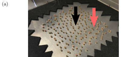
We perform measurements on five different configurations $\chi=0.15,0.25,0.30,0.40$, and a triangular lattice. For all the samples studied, we kept the number density constant ($\rho\simeq 0.32$ cm^-2). The point patterns and the structure factors of the samples are shown in the Supplemental Material Fig. S2. The cavity can be considered as two dimensional for the microwave frequencies $\nu<10$ GHz studied. Under this condition, only the first transverse magnetic mode, TM₀, exists in air: the electric field is perpendicular to the plane, and the field amplitude is uniform over the cavity height Jackson 1998. We mimic an infinite 2D system by placing absorbing carbon loaded polyurethane foam between the sample and the metallic walls of the cavity. We raster the cavity with a mobile antenna that is inserted by a robotic arm through holes drilled into the upper plate with a diameter 2 mm, on a $5\times 5$ mm² grid unit cell. Considering the sample size, and the fact that we are not able to penetrate the cavity at the holes above the scatterers, we end up with about $\sim 2700$ measured positions.

At each grid point $(x,y)$, we measure the complex transmission spectrum $S_{12}(\nu)$ between a fixed antenna (1) placed at the center of the cavity and the mobile antenna (2) using a vector network analyzer. Figure 1(b) shows examples of measured spectra $|S_{12}(\nu)|^{2}$ between the central position $1$ and probe position $2$ for different $\chi$ values and for a given distance $d$ between the antennas. The small transmission values of order $10^{-6}$ or less are because the receiving antenna is weakly coupled to the cavity. The measured spectra consist of a superposition of peaks which are associated to the resonances of the system. We extract their frequency, complex amplitude and width using harmonic inversion as described in Ref. Main et al. 2000; Wiersig and Main 2008. We then cluster the resonances measured on all the lattice points in order to reveal all the eigenmodes present in the system without being spoiled by false resonances induced by noise (See Supplemental Material III.1 Maier and Slater 1952; Pourrajabi et al. 2014; Ruiz et al. 2007).

In Fig. 2, we plot a histogram of the frequencies of the eigenmodes, which is directly proportional to the density of states (DOS). We compare the results for SHU point patterns with different values of $\chi$, to the results obtained for a triangular lattice. As shown in earlier numerical work, the triangular lattice is the champion photonic crystal structure in 2D, with a gap slightly larger than disordered hyperuniform structures Froufe-Pérez et al. 2016. Our experimental data confirms the two first TM photonic band gaps predicted for the triangular lattice Joannopoulos et al. 2008. We also find frequency windows without states for the SHU disordered systems. Surprisingly, not only the first but also the second band gap is present in the $\chi=0.4$ sample. To our knowledge, second and higher order band gaps have so far neither been predicted nor observed in disordered systems. This finding is in contradiction to previous claims about the origin of band gaps in disordered photonic materials Jin et al. 2001; Miyazaki et al. 2003; Rockstuhl et al. 2006. To corroborate additional evidence for this interesting observation, we performed band structure calculations, using the same parameters as in the experiment (see Supplemental Material §. IV Johnson and Joannopoulos 2001). These numerical data confirm the existence of a second-order band gap for $\chi\geq 0.4$. Both the first and the second gap approximately match the maxima of $S(k)$ of the triangular lattice and of the SHU structures, supporting earlier proposals that short-range spatial correlations play a key role for the opening of band-gaps in amorphous photonic materials Froufe-Pérez et al. 2016. Experimentally, we observe a narrow photonic band gap even for our most disordered sample ($\chi=0.15$). Our numerical data for a large ensemble of system realizations, however, suggest that the band gap closes for $\chi\lesssim 0.3$ and reduces to a pseudogap with a small but finite density of states. Naturally, variations between different realizations of hyperuniform materials become more pronounced for smaller values of $\chi$ (see Supplemental Material Fig. S5) and moreover the number of states per frequency bin is small for a finite sized system. This can lead to the situation that the central frequency and width of the band gaps depend on the precise realization of the point pattern, which is a distinct feature of disordered materials not found in crystals. For larger values of $\chi$ these variations are suppressed, and the gap becomes more robust against statistical fluctuations.

We now consider the optical properties of our material outside the gap Froufe-Pérez et al. 2017. The amplitude of the peaks observed in Fig. 1(b), and clustered to reveal the eigenmodes, differs from one position to the other and from this we obtain an electric field amplitude map $E_{\nu}(x,y)$ of an eigenmode Stein et al. 1995 (see Supplemental Material § III Maier and Slater 1952; Pourrajabi et al. 2014; Ruiz et al. 2007; Xeridat et al. 2009). These eigenmodes maps, shown in the first line of Fig. 3, reveal the striking variations in optical transport properties across the spectral range covered by our experiment.

At low frequencies, we observe simple square cavity modes as if the medium was homogeneous, which is a remarkable result given the fact that at $\nu\sim 2$GHz, the system size $L=25$ cm is almost two orders of magnitude larger than the Boltzmann mean free path $\ell_{\mathrm{s}}(\nu)$ of the cylinder ensemble (see Supplemental Material Fig. S1), with $\ell_{\mathrm{s}}(\nu)=[\sigma_{\mathrm{s}}(\nu)\rho]^{-1}$ given by the total scattering cross section $\sigma_{\mathrm{s}}(\nu)$ and the number density $\rho$. An alternative way to study wave propagation in the SHU material is to monitor the wave emitted by the central antenna as it propagates through the medium in the time domain. By calculating the real part of the Fourier-transform of $S_{12}(\nu)\times F_{f_{0},\Delta\nu}(\nu)$ (with $F_{f_{0},\Delta\nu}$ a band pass filter of bandwidth $\Delta\nu$ centered around $f_{0}$) at all points on the lattice, we reconstruct movies of the propagating electromagnetic fields as a function of time for the selected bandwidth $\Delta\nu$. Individual frames of the movies are shown in Figs. 3(f-j) (details on the numerical procedure and the entire movies are included in the Supplemental Material § V). Figure 3(f) shows that at low frequencies a circular wave propagates from the central antenna into the medium again signaling transparency. Note that the disordered pattern observed at $t_{3}$ in Fig. 3(f) is due to the nonperfectly absorbing foams placed around the sample which reflect part of the signal (for more details, see Supplemental Material Videos S6-1 and S6-2). From the velocity of the circular wave in the medium we can derive the effective refractive index of the samples and find $n_{\mathrm{eff}}\sim 1.8$. Equally, counting the nodal lines of the modes (Fig. 3(a)) and relating them to their frequencies, we obtain values of the effective refractive index of the metamaterial in the range $n_{\mathrm{eff}}=1.7\pm 0.3$. The uncertainty is due to the fact that, for disordered systems, the cavity size is not well defined and moreover, we observe a slight increase of $n_{\mathrm{eff}}$ from $\nu=1\to 3$ GHz. For comparison, the Maxwell-Garnett effective refractive index, which in 2D corresponds to the square root of the surface averaged permittivity, is $n_{\text{MG}}=2.05$.

Torquato and coworkers named their designer materials “stealthy” hyperuniform because they predicted them to be fully transparent below a threshold frequency $\nu<\nu_{\mathrm{c}}$ Batten et al. 2008. The latter is equivalent to saying that $L/\ell^{\star}\to 0$ (with $\ell^{\star}$ the transport mean free path), while $L/\ell_{\mathrm{s}}$ remains finite and can even be larger than one. In this first-order or single-scattering approximation $\nu_{\mathrm{c}}=\frac{c}{n_{\mathrm{eff}}}\sqrt{\frac{\rho\chi}{\pi}}$ Froufe-Pérez et al. 2017. For our system parameters, the theoretical $\nu_{\mathrm{c}}$ range from $\simeq 2.2$ GHz ($\chi=0.15$) to $\simeq 3.0$ GHz ($\chi=0.4$) based on an effective refractive index of $n_{\mathrm{eff}}\sim 1.8$. Leseur et al. 2016 demonstrated recently that stealthy transparency is also robust against recurrent multiple scattering. They establish a stricter criterion for transparency, $L/\ell_{\mathrm{s}}\ll k\ell_{\mathrm{s}}$, in a dense SHU disordered material composed of dipolar point scatterers. While transparency is retained under this condition it also implies that the transition at $\nu_{\mathrm{c}}$ is not sharp but system size dependent. From a theoretical evaluation of $\sigma_{\mathrm{s}}(\nu)$ for our $\varepsilon=36$ cylinders in air, however, we find that only for $\nu<1$ GHz the condition $L/\ell_{\mathrm{s}}<k\ell_{\mathrm{s}}$ is met (see Supplemental Material Fig. S1 Bohren and Huffman 1998). The experimental results, however, suggest that the condition set by Leseur et al. 2016 is too restrictive and transparency remains a robust feature for $\nu<\nu_{\mathrm{c}}$ in our dense, high index SHU materials, even for $k\ell_{\mathrm{s}}\lesssim 1$ (see also Supplemental Material Fig. S7).

For frequencies $\nu>\nu_{\mathrm{c}}$ transparency is clearly lost and we observe scattering and wave diffusion. The modes become disordered, Fig. 3(b), and the propagating wavefronts in the time domain are highly distorted signaling mean free paths smaller than the system size, Fig. 3(g). A closer inspection of the propagating wave fronts, Supplemental Material Fig. S7, illustrates how the onset of scattering and wave diffusion is shifted to higher frequencies $\nu_{\mathrm{c}}(\chi)\propto\sqrt{\chi}$ as the system becomes more and more stealthy. At frequencies close to the first band gap, we observe spatially localized modes as shown in Figs. 3(c) and (d) Laurent et al. 2007; Le Thomas et al. 2009; García et al. 2012. In the time domain, we find that, at longer times, the wave stays localized near the central antenna, as shown in the panels framed red in Figs. 3(h,i) and in the corresponding Supplemental Material videos S6-4 and S6-6.

We note that the modes below the band gap are localized on the dielectric cylinders, Fig. 3(c), and the modes above the band gap are localized in air, Fig. 3(d). For frequencies in between the first and the second band gap we again observe diffusive modes, Fig. 3(e), as well as extended waves at later times, Fig. 3(j). For frequencies in the band gaps we find no modes, all positions are phase coherent and there is no propagation.

Next, we calculate the Thouless conductance $g_{\mathrm{Th}}=\delta\nu/\Delta\nu$, which is a fundamental localization parameter Thouless 1977; Wang and Genack 2011; Mondal et al. 2019. Thouless argued that in the Anderson localization regime, the dimensionless ratio $g_{\mathrm{Th}}=\delta\nu/\Delta\nu$ falls below unity. In this case, the spectral widths $\delta\nu$ of the modes are smaller than their spacing $\Delta\nu$, and the modes are isolated Thouless 1977. In the opposite limit, for $g_{\mathrm{Th}}\geq 1$ modes overlap and waves can propagate. By calculating the average width of the modes in each frequency bin, Fig. 2, we extract the mean Thouless conductance for each frequency bin as shown in Fig. 4. We have marked the data points directly at the band edges by open circles in Fig. 4. Note that, due to the discretization, their values can be affected by the zeroes of the DOS in the gap. Inside the band gap there are no modes and $\left<g_{\mathrm{Th}}\right>$ is not defined. We find values of $\left<g_{\mathrm{Th}}\right>\sim 1$ everywhere except in the vicinity of the gap where $\left<g_{\mathrm{Th}}\right>$ drops by up to two orders of magnitude, signaling localization. This result is consistent with both the finite spatial extension of the modes we observe experimentally, see Figs. 3(c,d), and the localization of the propagating wave in the same frequency domain, Fig. 3(h,i). In the low-frequency regime, the Thouless conductance is close to one, and wave transport expands over the whole system size.

In conclusion, we show experimentally that disordered dielectric structures display different characteristic transport regimes such as transparency, photon diffusion, Anderson localization, as well as first and even second order band gaps. We rationalize our findings by analyzing the mode structure and the propagation of waves in the time domain. We find evidence that transparency is robust against recurrent multiple scattering, and that the stealthy materials we study retain their low-frequency transparency even for the unusually strong refractive index mismatch between our scatterers and air $\sqrt{\varepsilon/\varepsilon_{\text{air}}}=6$. Our results lend support to recent numerical predictions and shed new light on the interplay between disorder and correlations Froufe-Pérez et al. 2017. We believe this will have significant consequences for the design of photonic materials, such as two-dimensional nanostructured materials for light harvesting in solar cells Vynck et al. 2012 or light guiding in all-optical circuit applications Milošević et al. 2019.

References

- Yablonovitch (1987) E. Yablonovitch, Inhibited spontaneous emission in solid-state physics and electronics, Phys. Rev. Lett. 58, 2059 (1987).
- John (1987) S. John, Strong localization of photons in certain disordered dielectric superlattices, Phys. Rev. Lett. 58, 2486 (1987).
- Joannopoulos et al. (2008) J. Joannopoulos, S. Johnson, J. Winn, and R. Meade, Photonic Crystals: Molding the Flow of Light, 2nd ed. (Princeton University Press, Princeton (New Jersey), 2008).
- Vynck et al. (2009) K. Vynck, D. Felbacq, E. Centeno, A. I. Căbuz, D. Cassagne, and B. Guizal, All-dielectric rod-type metamaterials at optical frequencies, Phys. Rev. Lett. 102, 133901 (2009).
- Zoorob et al. (2000) M. E. Zoorob, M. D. B. Charlton, G. J. Parker, J. J. Baumberg, and M. C. Netti, Complete photonic bandgaps in 12-fold symmetric quasicrystals, Nature 404, 740 (2000).
- Jin et al. (2001) C. Jin, X. Meng, B. Cheng, Z. Li, and D. Zhang, Photonic gap in amorphous photonic materials, Phys. Rev. B 63, 195107 (2001).
- Florescu et al. (2009) M. Florescu, S. Torquato, and P. J. Steinhardt, Designer disordered materials with large, complete photonic band gaps, Proceedings of the National Academy of Sciences 106, 20658 (2009).
- Liew et al. (2011) S. F. Liew, J.-K. Yang, H. Noh, C. F. Schreck, E. R. Dufresne, C. S. O’Hern, and H. Cao, Photonic band gaps in three-dimensional network structures with short-range order, Phys. Rev. A 84, 063818 (2011).
- Froufe-Pérez et al. (2016) L. S. Froufe-Pérez, M. Engel, P. F. Damasceno, N. Muller, J. Haberko, S. C. Glotzer, and F. Scheffold, Role of short-range order and hyperuniformity in the formation of band gaps in disordered photonic materials, Phys. Rev. Lett. 117, 053902 (2016).
- Froufe-Pérez et al. (2017) L. S. Froufe-Pérez, M. Engel, J. J. Sáenz, and F. Scheffold, Band gap formation and Anderson localization in disordered photonic materials with structural correlations, Proceedings of the National Academy of Sciences 114, 9570 (2017).
- Yang et al. (2010) J.-K. Yang, C. Schreck, H. Noh, S.-F. Liew, M. I. Guy, C. S. O’Hern, and H. Cao, Photonic-band-gap effects in two-dimensional polycrystalline and amorphous structures, Phys. Rev. A 82, 053838 (2010).
- Marichy et al. (2016) C. Marichy, N. Muller, L. S. Froufe-Pérez, and F. Scheffold, High-quality photonic crystals with a nearly complete band gap obtained by direct inversion of woodpile templates with titanium dioxide, Scientific Reports 6, 21818 (2016).
- Torquato and Stillinger (2003) S. Torquato and F. H. Stillinger, Local density fluctuations, hyperuniformity, and order metrics, Phys. Rev. E 68, 041113 (2003).
- Uche et al. (2004) O. U. Uche, F. H. Stillinger, and S. Torquato, Constraints on collective density variables: Two dimensions, Phys. Rev. E 70, 046122 (2004).
- Sperling et al. (2016) T. Sperling, L. Schertel, M. Ackermann, G. J. Aubry, C. Aegerter, and G. Maret, Can 3D light localization be reached in ‘white paint’?, New Journal of Physics 18, 013039 (2016), 1510.08092 .
- Laurent et al. (2007) D. Laurent, O. Legrand, P. Sebbah, C. Vanneste, and F. Mortessagne, Localized Modes in a Finite-Size Open Disordered Microwave Cavity, Phys. Rev. Lett. 99, 253902 (2007).
- Jackson (1998) J. D. Jackson, Classical Electrodynamics, 3rd ed. (John Wiley & Sons, Inc., New York, 1998).
- Main et al. (2000) J. Main, P. A. Dando, D. Belkic, and H. S. Taylor, Decimation and harmonic inversion of periodic orbit signals, Journal of Physics A: Mathematical and General 33, 1247 (2000).
- Wiersig and Main (2008) J. Wiersig and J. Main, Fractal Weyl law for chaotic microcavities: Fresnel’s laws imply multifractal scattering, Phys. Rev. E 77, 036205 (2008).
- Maier and Slater (1952) L. C. Maier and J. C. Slater, Field strength measurements in resonant cavities, Journal of Applied Physics 23, 68 (1952).
- Pourrajabi et al. (2014) M. Pourrajabi, D. Moulavi, R. J. G. B. Campello, A. Zimek, J. Sander, and R. Goebel, Model selection for semi-supervised clustering, in Advances in Database Technology – EDBT 2014, edited by S. Amer-Yahia, V. Christophides, A. Kementsietsidis, M. Garofalakis, S. Idreos, and V. Leroy (OpenProceedings.org, Konstanz, 2014) pp. 331–342.
- Ruiz et al. (2007) C. Ruiz, M. Spiliopoulou, and E. Menasalvas, C-DBSCAN: Density-based clustering with constraints, in Rough Sets, Fuzzy Sets, Data Mining and Granular Computing, edited by A. An, J. Stefanowski, S. Ramanna, C. J. Butz, W. Pedrycz, and G. Wang (Springer Berlin Heidelberg, Berlin, Heidelberg, 2007) pp. 216–223.
- Miyazaki et al. (2003) H. Miyazaki, M. Hase, H. T. Miyazaki, Y. Kurokawa, and N. Shinya, Photonic material for designing arbitrarily shaped waveguides in two dimensions, Phys. Rev. B 67, 235109 (2003).
- Rockstuhl et al. (2006) C. Rockstuhl, U. Peschel, and F. Lederer, Correlation between single-cylinder properties and bandgap formation in photonic structures, Opt. Lett. 31, 1741 (2006).
- Johnson and Joannopoulos (2001) S. G. Johnson and J. D. Joannopoulos, Block-iterative frequency-domain methods for Maxwell’s equations in a planewave basis, Opt. Express 8, 173 (2001).
- Stein et al. (1995) J. Stein, H.-J. Stöckmann, and U. Stoffregen, Microwave studies of billiard green functions and propagators, Phys. Rev. Lett. 75, 53 (1995).
- Xeridat et al. (2009) O. Xeridat, C. Poli, O. Legrand, F. Mortessagne, and P. Sebbah, Quasimodes of a chaotic elastic cavity with increasing local losses, Phys. Rev. E 80, 035201(R) (2009).
- Batten et al. (2008) R. D. Batten, F. H. Stillinger, and S. Torquato, Classical disordered ground states: Super-ideal gases and stealth and equi-luminous materials, Journal of Applied Physics 104, 033504 (2008).
- Leseur et al. (2016) O. Leseur, R. Pierrat, and R. Carminati, High-density hyperuniform materials can be transparent, Optica 3, 763 (2016).
- Bohren and Huffman (1998) C. F. Bohren and D. R. Huffman, Absorption and Scattering of Light by Small Particles (Wiley, New York, 1998).
- Le Thomas et al. (2009) N. Le Thomas, R. Houdré, D. M. Beggs, and T. F. Krauss, Fourier space imaging of light localization at a photonic band-edge located below the light cone, Phys. Rev. B 79, 033305 (2009).
- García et al. (2012) P. D. García, S. Stobbe, I. Söllner, and P. Lodahl, Nonuniversal intensity correlations in a two-dimensional Anderson-localizing random medium, Phys. Rev. Lett. 109, 253902 (2012).
- Thouless (1977) D. J. Thouless, Maximum metallic resistance in thin wires, Phys. Rev. Lett. 39, 1167 (1977).
- Wang and Genack (2011) J. Wang and A. Z. Genack, Transport through modes in random media, Nature 471, 345 (2011).
- Mondal et al. (2019) S. Mondal, R. Kumar, M. Kamp, and S. Mujumdar, Optical Thouless conductance and level-spacing statistics in two-dimensional Anderson localizing systems, Phys. Rev. B 100, 060201(R) (2019).
- Vynck et al. (2012) K. Vynck, M. Burresi, F. Riboli, and D. S. Wiersma, Photon management in two-dimensional disordered media, Nature Materials 11, 1017 (2012).
- Milošević et al. (2019) M. M. Milošević, W. Man, G. Nahal, P. J. Steinhardt, S. Torquato, P. M. Chaikin, T. Amoah, B. Yu, R. A. Mullen, and M. Florescu, Hyperuniform disordered waveguides and devices for near infrared silicon photonics, Scientific Reports 9, 20338 (2019).
Supplementary Material
This document contains the scattering properties of a single rod, details on the structures of the point patterns, the band structure calculation, details on the time domain propagation videos and all the technical information on the data analysis. The seven videos (permanently stored on the Zenodo repository: https://doi.org/10.5281/zenodo.3978032) show how the electromagnetic wave propagates in the cavity for different frequency ranges (see Supplemental Material Fig. S6 for the description of the videos).
I Boltzmann scattering mean free path.
In Fig. S1 we show the scattering efficiency of an individual cylinder in TM polarization calculated using Mie theory Bohren and Huffman 1998 (upper panel). In the lower panel, we show how the corresponding Boltzmann scattering mean free path (with the total scattering cross section) compares with , the size of the system, and , the wavelength in vacuum of the wave.
II Point patterns and their structure factors.
Figure S2(a) shows the point patterns of the samples studied in this study, and Fig. S2(b) the corresponding average structure factors