跳到论文正文
W Papers独立论文阅读器 arXiv:2003.00738 论文正文 计算阅读时间 · 0%
引用这篇论文根据当前论文元数据生成,正式投稿前建议核对。


License: arXiv.org perpetual non-exclusive license
arXiv:2003.00738v1 [stat.ML] 02 Mar 2020

Analysis via Orthonormal Systems in Reproducing Kernel Hilbert C∗C^{*}-Modules and Applications

Yuka Hashimoto Affiliation: NTT Network Technology Laboratories, NTT Corporation, Tokyo, Japan Affiliation: Graduate School of Science and Technology, Keio University, Kanagawa, Japan Correspondence to: yuka.hashimoto.rw@hco.ntt.co.jp    Isao Ishikawa Affiliation: Faculty of Science and Technology, Keio University, Kanagawa, Japan Affiliation: Center for Advanced Intelligence Project, RIKEN, Tokyo, Japan    Masahiro Ikeda Affiliation: Faculty of Science and Technology, Keio University, Kanagawa, Japan Affiliation: Center for Advanced Intelligence Project, RIKEN, Tokyo, Japan    Fuyuta Komura Affiliation: Graduate School of Science and Technology, Keio University, Kanagawa, Japan Affiliation: Center for Advanced Intelligence Project, RIKEN, Tokyo, Japan    Takeshi Katsura Affiliation: Faculty of Science and Technology, Keio University, Kanagawa, Japan Affiliation: Center for Advanced Intelligence Project, RIKEN, Tokyo, Japan    Yoshinobu Kawahara Affiliation: Institute of Mathematics for Industry, Kyushu University, Fukuoka, Japan Affiliation: Center for Advanced Intelligence Project, RIKEN, Tokyo, Japan
Abstract

Kernel methods have been among the most popular techniques in machine learning, where learning tasks are solved using the property of reproducing kernel Hilbert space (RKHS). In this paper, we propose a novel data analysis framework with reproducing kernel Hilbert C∗C^{*}-module (RKHM), which is another generalization of RKHS than vector-valued RKHS (vv-RKHS). Analysis with RKHMs enables us to deal with structures among variables more explicitly than vv-RKHS. We show the theoretical validity for the construction of orthonormal systems in Hilbert C∗C^{*}-modules, and derive concrete procedures for orthonormalization in RKHMs with those theoretical properties in numerical computations. Moreover, we apply those to generalize with RKHM kernel principal component analysis and the analysis of dynamical systems with Perron-Frobenius operators. The empirical performance of our methods is also investigated by using synthetic and real-world data.

Keywords: 
kernel method, RKHM, structured data, principal component analysis, interacting dynamical system

1 Introduction

Kernel methods have been among the most popular techniques in machine learning (cf. (Schölkopf & Smola 2001)), where learning tasks are solved using the property of reproducing kernel Hilbert space (RKHS). RKHS is the space of complex-valued functions equipped with an inner product that is determined with a positive-definite kernel. Here, the orthonormality is defined on the basis of the inner products calculated by evaluating a kernel function, which plays an important role in developing practical algorithms.

Whereas almost all the classical literature on RKHS approaches has focused on complex-valued functions, RKHSs of vector-valued functions, i.e., vector-valued RKHSs (vv-RKHSs), have received increasing attention (Micchelli & Pontil 2005; Álvarez et al. 2011; Lim et al. 2015; Minh et al. 2016; Kadri et al. 2016). This paradigm allows us to incorporate information about structures among observation variables into analyses with RKHSs. Many kernel methods such as SVM can be generalized to vector-valued functions by employing vv-RKHSs (Minh et al. 2016).

However, the use of vv-RKHS may not always be the best option to analyze structured data, mainly for two reasons. First, although a sample is transformed into a unique function in RKHSs, a function in vv-RKHSs corresponding to a sample cannot be determined uniquely. Second, although for each sample composed of several elements, relations between all combinations of pairs of the elements should not be lost, information about the relations may be lost and can be difficult to recover when using vv-RKHSs. This is caused by the fact that an inner product in vv-RKHSs, which measures the similarity between a pair of samples in data, is represented with one complex value.

In this paper, we propose a data analysis framework with reproducing kernel Hilbert C∗C^{*}-module (RKHM), which is another generalization of RKHS. The theory of RKHM was originally studied in mathematical physics to analyze covariance kernels arising in the theory of generalized stochastic processes and the dilations of operators (Itoh 1990; Heo 2008). Unlike vv-RKHSs, the theory of RKHMs enables us to transform each sample as a unique C∗C^{*}-algebra-valued function, with C∗C^{*}-algebra-valued inner products. A C∗C^{*}-algebra is a generalization of the space of complex values. An example of C∗C^{*}-algebra is the space of matrices. Therefore, we can define a matrix-valued inner product that encodes the similarities of all combinations of pairs of variables in data.

As well as RKHS, the construction of orthonormal systems plays an important role in applying the theory of RKHMs to algorithm developments. To the best of our knowledge, although the generalization of the notion of orthonormal to C∗C^{*}-algebra-valued inner-products has been proposed in mathematics (Bakić & Guljaš 2001), its application to data analysis has not been discussed so far. Meanwhile, as for theoretical analyses of RKHMs for data analysis, we can find the only literature by Ye 2017, where only the case of RKHMs for data represented as matrices is considered without addressing orthonormality. Thus, its applicability to data analysis is limited. In this paper, we develop novel algorithms using RKHMs through the construction of orthonormal systems with C∗C^{*}-algebra-valued inner-products. We first show the theoretical validity for constructing orthonormal systems in Hilbert C*-modules. Then, we derive concrete procedures for orthonormalization in RKHMs and show some theoretical results on those properties in the numerical computations. Moreover, we apply those to generalize with RKHM kernel principal component analysis (PCA) and the analysis of dynamical systems with Perron-Frobenius operators, under the motivation described above. Note that the generalizations are not straightforward because an element of C∗C^{*}-algebra is not always commutative or invertible. However, our generalizations based on the developed theories enable us to access and extract rich information in structured data, which is shown partly here in the context of PCA and the analysis of interacting dynamical systems. Note that, to the best of our knowledge, this is the first paper to describe practical algorithms to utilize the notion of orthonormal with respect to C∗C^{*}-algebra-valued inner products in RKHMs for the analysis of structured data.

The remainder of this paper is organized as follows. First, in Section 2, we briefly review the theory of RKHMs. In Section 3, we introduce the definition of the orthonormality with C∗C^{*}-algebra-valued inner products and then show the theoretical validity to consider it. In Section 4, we derive concrete procedures for constructing orthonormal systems in RKHMs with theoretical analyses in their numerical computations. In Sections 5 and 6, we develop the applications of the developed results to generalize with RKHM kernel PCA and the analysis of dynamical systems with Perron-Frobenius operators, respectively. Finally, we empirically investigate the performance of our methods in Section 7 and conclude the paper in Section 8. The notations in this paper are explained in Appendix A, and all proofs are given in Appendix I in the supplementary material.

2 Backgrounds

In this section, we first briefly review C∗C^{*}-algebras and C∗C^{*}-modules in Section 2.1, and RKHMs in Subection 2.2. The precise statements and definitions about them are detailed in Appendix D. RKHMs are generalizations of RKHSs. The theoretical backgrounds of RKHSs are given in Appendices B. We also add a review on vv-RKHSs, which are other generalizations of RKHSs, in Appendix C.

2.1 C∗C^{*}-algebra and C∗C^{*}-module

A C∗C^{*}-algebra and a C∗C^{*}-module are suitable generalizations of the space of complex numbers ℂ\mathbb{C} and a vector space, respectively. In this paper, we denote a C∗C^{*}-algebra by 𝒜\mathcal{A} and a C∗C^{*}-module by ℳ\mathcal{M}, respectively. As we see below, many complex-valued notions can be generalized to 𝒜\mathcal{A}-valued.

Mathematically, a C∗C^{*}-algebra is defined as a Banach space equipped with a product structure and an involution (⋅)∗:𝒜→𝒜(\cdot)^{*}:\mathcal{A}\rightarrow\mathcal{A} (Definition D.1). We denote the norm of 𝒜\mathcal{A} by ∥⋅∥𝒜\|\cdot\|_{\mathcal{A}}. A main example of C∗C^{*}-algebras is the space of matrices ℂm×m\mathbb{C}^{m\times m}. In this case, the product structure is the usual product of matrices, the involution is the Hermitian conjugate, and the norm ∥⋅∥𝒜\|\cdot\|_{\mathcal{A}} is the operator norm.

The notion of positiveness (Definition D.2) is also important in C∗C^{*}-algebras. We denote c≥0c\geq 0 if c∈𝒜c\in\mathcal{A} is positive. In the case of 𝒜=ℂm×m\mathcal{A}=\mathbb{C}^{m\times m}, the positiveness corresponds to Hermitian positive semi-definiteness of matrices. The notion of positiveness provides us the (pre) order in 𝒜\mathcal{A}, and thus, enables us to consider optimization problems in 𝒜\mathcal{A}.

A C∗C^{*}-module ℳ\mathcal{M} over 𝒜\mathcal{A} (Definition D.5) is a linear space ℳ\mathcal{M} equipped with a right 𝒜\mathcal{A}-multiplication. For u∈ℳ,c∈𝒜u\in\mathcal{M},c\in\mathcal{A}, the right 𝒜\mathcal{A}-multiplication of uu with cc is denoted as u​cuc.

A linear map K:ℳ→ℳK:\mathcal{M}\to\mathcal{M} is called an 𝒜\mathcal{A}-linear map if K⁡(u​c)=(K​u)​cK(uc)=(Ku)c holds for any u∈ℳu\in\mathcal{M} and c∈𝒜c\in\mathcal{A}.

2.2 C∗C^{*}-algebra-valued inner product and RKHM

We consider an 𝒜\mathcal{A}-valued inner product in ℳ\mathcal{M}, which is a straightforward generalization of a complex-valued one.

Definition 2.1 (𝒜\mathcal{A}-valued inner product).

A map ⟨⋅,⋅⟩:ℳ×ℳ→𝒜\left\langle\cdot,\cdot\right\rangle:\mathcal{M}\times\mathcal{M}\to\mathcal{A} is called an 𝒜\mathcal{A}-valued inner product if it satisfies the following properties for u,v,w∈ℳu,v,w\in\mathcal{M} and c,d∈𝒜c,d\in\mathcal{A}:

1. ⟨u,v​c+w​d⟩=⟨u,v⟩​c+⟨u,w⟩​d\left\langle u,vc+wd\right\rangle=\left\langle u,v\right\rangle c+\left\langle u,w\right\rangle d ,
2. ⟨v,u⟩=⟨u,v⟩∗\left\langle v,u\right\rangle=\left\langle u,v\right\rangle^{*} ,
3. ⟨u,u⟩≥0\left\langle u,u\right\rangle\geq 0 and if ⟨u,u⟩=0\left\langle u,u\right\rangle=0 then u=0u=0 .

For u∈ℳu\in\mathcal{M}, we define the 𝒜\mathcal{A}-valued absolute value |u||u| on ℳ\mathcal{M} by the positive element |u||u| of 𝒜\mathcal{A} such that |u|2=⟨u,u⟩|u|^{2}=\left\langle u,u\right\rangle. Since |⋅||\cdot| takes values in more structured space 𝒜\mathcal{A}, it behaves more complicatedly, but provides us with more information.

The 𝒜\mathcal{A}-valued absolute value |⋅||\cdot| defines a norm ∥⋅∥\|\cdot\| on ℳ\mathcal{M} by ‖u‖:=‖|u|‖𝒜\|u\|:=\big\||u|\big\|_{\mathcal{A}}. By definition, the norm ∥⋅∥\|\cdot\| is regarded as an aspect of the 𝒜\mathcal{A}-valued absolute value |⋅||\cdot|. We call ℳ\mathcal{M} equipped with ⟨⋅,⋅⟩\left\langle\cdot,\cdot\right\rangle a Hilbert C∗C^{*}-module if ℳ\mathcal{M} is complete w.r.t. the norm ∥⋅∥\|\cdot\|. An RKHM is an example of Hilbert C∗C^{*}-modules. Another example is 𝒜n\mathcal{A}^{n} (Lemma D.13), which is utilized for orthonormalization (Remark 4.7).

We now summarize the theory of RKHMs, which is discussed, for example, in (Heo 2008). Similar to the case of RKHSs, we begin with an 𝒜\mathcal{A}-valued generalization of a positive definite kernel on a non-empty set 𝒴\mathcal{Y}.

Definition 2.2 (𝒜\mathcal{A}-valued positive definite kernel).

An 𝒜\mathcal{A}-valued map k:𝒴×𝒴→𝒜k:\ \mathcal{Y}\times\mathcal{Y}\to\mathcal{A} is called a positive definite kernel if it satisfies the following conditions:

1. k⁡(x,y)=k​(y,x)∗k(x,y)=k(y,x)^{*}  for x,y∈𝒴x,y\in\mathcal{Y},
2. ∑t,s=1nct∗​k​(xt,xs)​cs≥0\sum_{t,s=1}^{n}c_{t}^{*}k(x_{t},x_{s})c_{s}\geq 0  for n∈ℕn\in\mathbb{N}, c1,…,cn∈𝒜c_{1},\ldots,c_{n}\in\mathcal{A}, x1,…,xn∈𝒴x_{1},\ldots,x_{n}\in\mathcal{Y}.

We remark that in the case where 𝒜\mathcal{A} is the space of bounded linear operators on a Hilbert space, Definition 2.2 is equivalent to the operator valued positive definite kernel for the theory of vv-RKHSs (Lemma D.9).

Let ϕ:𝒴→𝒜𝒴\phi:\mathcal{Y}\to\mathcal{A}^{\mathcal{Y}} be the feature map associated with kk, which is defined as ϕ⁡(x)=k⁡(⋅,x)\phi(x)=k(\cdot,x) for x∈𝒴x\in\mathcal{Y}. Similar to the case of RKHSs, we construct the following C∗C^{*}-module composed of 𝒜\mathcal{A}-valued functions by means of ϕ\phi:

ℳk,0:={∑t=1nϕ(xt)ct|n∈ℕ,ct∈𝒜,xt∈𝒴}.\mathcal{M}_{k,0}:=\bigg\{\sum_{t=1}^{n}\phi(x_{t})c_{t}\bigg|\ n\in\mathbb{N},\ c_{t}\in\mathcal{A},\ x_{t}\in\mathcal{Y}\bigg\}.

An 𝒜\mathcal{A}-valued map ⟨⋅,⋅⟩k:ℳk,0×ℳk,0→𝒜\left\langle\cdot,\cdot\right\rangle_{k}:\mathcal{M}_{k,0}\times\mathcal{M}_{k,0}\to\mathcal{A} is defined as follows with kk:

⟨∑s=1nϕ⁡(xs)​cs,∑t=1lϕ⁡(yt)​dt⟩k:=∑s=1n∑t=1lcs∗​k​(xs,yt)​dt.\bigg\langle\sum_{s=1}^{n}\phi(x_{s})c_{s},\sum_{t=1}^{l}\phi(y_{t})d_{t}\bigg\rangle_{k}:=\sum_{s=1}^{n}\sum_{t=1}^{l}c_{s}^{*}k(x_{s},y_{t})d_{t}.

By the properties in Definition 2.2 of kk, ⟨⋅,⋅⟩k\left\langle\cdot,\cdot\right\rangle_{k} is well-defined and has the reproducing property. Also, it satisfies the properties in Definition 2.1 (Proposition D.10). Therefore, ⟨⋅,⋅⟩k\left\langle\cdot,\cdot\right\rangle_{k} is an 𝒜\mathcal{A}-valued inner product.

The reproducing kernel Hilbert 𝒜\mathcal{A}-module (RKHM) associated with kk is defined as the completion of ℳk,0\mathcal{M}_{k,0}. Similar to the cases of RKHSs, ⟨⋅,⋅⟩k\left\langle\cdot,\cdot\right\rangle_{k} is extended continuously to the RKHM and has the reproducing property (Proposition D.11). Also, the RKHM is uniquely determined (Proposition D.12).

We denote by ℳk\mathcal{M}_{k} the RKHM associated with kk. We also denote by |⋅|k|\cdot|_{k} and ∥⋅∥k\|\cdot\|_{k} the absolute value and norm on ℳk\mathcal{M}_{k}, respectively.

3 Orthonormality with C∗C^{*}-algebra-valued Inner Products

In this section, we define the orthonormality for C∗C^{*}-algebra-valued inner products, and develop theoretical foundations of its validity to apply it to the analysis of structured data.

Orthonormality plays an important role in data analysis because an orthonormal basis constructs orthogonal projections and an orthogonally projected vector minimizes the deviation from its original vector in the projected space.

We begin with, the definition of an orthonormal system and orthonormal basis in a Hilbert C∗C^{*}-module ℳ\mathcal{M}. We refer to, for example, Definition 1.2 in (Bakić & Guljaš 2001).

Definition 3.1 (Normalized).

A vector q∈ℳq\in\mathcal{M} is normalized if 0≠⟨q,q⟩=⟨q,q⟩20\neq\left\langle q,q\right\rangle=\left\langle q,q\right\rangle^{2}.

Note that in the case of a general C∗C^{*}-valued-inner product, for a normalized vector qq , ⟨q,q⟩\left\langle q,q\right\rangle is not always equal to the identity of 𝒜\mathcal{A} in contrast to the case of a complex-valued inner product.

Definition 3.2 (Orthonormal system and basis).

Let 𝒯\mathcal{T} be an index set. A set 𝒮={qt}t∈𝒯⊆ℳ\mathcal{S}=\{q_{t}\}_{t\in\mathcal{T}}\subseteq\mathcal{M} is called an orthonormal system (ONS) of ℳ\mathcal{M} if qtq_{t} is normalized for any t∈𝒯t\in\mathcal{T} and ⟨qs,qt⟩=0\left\langle q_{s},q_{t}\right\rangle=0 for s≠ts\neq t. We call 𝒮\mathcal{S} an orthonormal basis (ONB) if 𝒮\mathcal{S} is an orthonormal system and dense in ℳ\mathcal{M}.

We show basic properties of the above orthonormal systems. First, we derive the existence of an orthonormal basis.

Proposition 3.3.

The Hilbert C∗C^{*}-module over ℂm×m\mathbb{C}^{m\times m} has an orthonormal basis.

Unlike Hilbert spaces, Hilbert C∗C^{*}-modules do not always have an orthonormal basis for general 𝒜\mathcal{A} (Lance 1995; Landi & Pavlov 2009). However, Proposition 3.3 guarantees the validity of considering orthonormal bases in RKHMs over ℂm×m\mathbb{C}^{m\times m} for practical applications. Next, we show a minimization property.

Proposition 3.4.

Let {qt}t∈𝒯\{q_{t}\}_{t\in\mathcal{T}} be an orthonormal system of ℳ\mathcal{M} and let 𝒱\mathcal{V} be the completion of the space spanned by {qt}t∈𝒯\{q_{t}\}_{t\in\mathcal{T}}. For w∈ℳkw\in\mathcal{M}_{k}, let P:ℳ→𝒱P:\mathcal{M}\to\mathcal{V} be the projection operator defined as P​w:=∑t∈𝒯qt​⟨qt,w⟩Pw:=\sum_{t\in\mathcal{T}}q_{t}\left\langle q_{t},w\right\rangle. Then P​wPw is the unique solution of the following minimization problem:

minv∈𝒱⁡|w−v|2\min_{v\in\mathcal{V}}|w-v|^{2} (1)

Unlike the case of complex-valued inner products, the existence of the solution of 𝒜\mathcal{A}-valued minimization problem (1) is not obvious since the positive elements in 𝒜\mathcal{A} are not totally ordered. However, Proposition 3.4 shows the orthogonally projected vector uniquely minimizes the deviation from an original vector in 𝒱\mathcal{V}.

4 Matrix-valued Positive Definite Kernel and Orthonormality in RKHMs

In this section, we first construct a ℂm×m\mathbb{C}^{m\times m}-valued positive definite kernel, which encodes the similarities between all combinations of pairs (m2m^{2} pairs) of elements for two samples, each of which is composed of mm elements, in Section 4.1. Then, in Section 4.2, we develop theoretical foundations for calculating the orthonormalization in RKHMs.

4.1 Matrix-valued positive definite kernel

First, we introduce a matrix-valued positive definite kernel. Let 𝒳\mathcal{X} be a topological space. We consider data composed of mm elements of 𝒳\mathcal{X}. Let k~:𝒳×𝒳→ℂ\tilde{k}:\mathcal{X}\times\mathcal{X}\to\mathbb{C} be a complex-valued positive definite kernel, ϕ~\tilde{\phi} be the feature map, and ℋk~\mathcal{H}_{\tilde{k}} be the RKHS associated with k~\tilde{k}. On the basis of the above setting for 𝒳\mathcal{X} and RKHSs, we introduce a ℂm×m\mathbb{C}^{m\times m}-valued positive definite kernel kk, which is also proposed in the framework of vv-RKHSs (Lim et al. 2015), to construct an RKHM.

Lemma 4.1.

Let k:𝒳m×𝒳m→ℂm×mk:\mathcal{X}^{m}\times\mathcal{X}^{m}\to\mathbb{C}^{m\times m} be a matrix valued map where the (i,j)(i,j)-elements of k⁡(x1,x2)k(x_{1},x_{2}) are defined as k~​(x1,i,x2,j)\tilde{k}(x_{1,i},x_{2,j}) for xt=[xt,1,…,xt,m]∈𝒳mx_{t}=[x_{t,1},\ldots,x_{t,m}]\in\mathcal{X}^{m} for t=1,2t=1,2. Then, kk is a ℂm×m\mathbb{C}^{m\times m}-valued positive definite kernel.

The (i,j)(i,j)-element of k⁡(x1,x2)k(x_{1},x_{2}) for x1,x2∈𝒳mx_{1},x_{2}\in\mathcal{X}^{m} equals k~​(x1,i,x2,j)\tilde{k}(x_{1,i},x_{2,j}), which represents the similarities between x1,ix_{1,i} and x2,jx_{2,j} in ℋk~\mathcal{H}_{\tilde{k}}. Thus, the inner product between ϕ⁡(x1)\phi(x_{1}) and ϕ⁡(x2)\phi(x_{2}) describes the similarities of all combinations of pairs of elements of x1x_{1} and x2x_{2}.

4.2 Gram-Schmidt orthonormalization

We now consider the practical approach for orthonormalization with matrix-valued inner products.

Proposition 4.2 (Normalization).

Let ϵ≥0\epsilon\geq 0 and let q^∈ℳ\hat{q}\in\mathcal{M} satisfy ‖q^‖>ϵ\|\hat{q}\|>\epsilon. Then, there exists b^∈ℂm×m\hat{b}\in\mathbb{C}^{m\times m} such that ‖b^‖ℂm×m<1/ϵ\|\hat{b}\|_{\mathbb{C}^{m\times m}}<1/\epsilon and q:=q^​b^q:=\hat{q}\hat{b} is normalized. In addition, there exists b∈ℂm×mb\in\mathbb{C}^{m\times m} such that ‖q^−q​b‖≤ϵ\|\hat{q}-qb\|\leq\epsilon.

Sketch of the proof.

Let λ1≥…≥λm≥0\lambda_{1}\geq\ldots\geq\lambda_{m}\geq 0 be the eigenvelues of ⟨q^,q^⟩\left\langle\hat{q},\hat{q}\right\rangle. Since ⟨q^,q^⟩\left\langle\hat{q},\hat{q}\right\rangle is positive, there exists an unitary matrix cc such that ⟨q^,q^⟩=c∗​diag⁡{λ1,…,λm}​c\left\langle\hat{q},\hat{q}\right\rangle=c^{*}\operatorname{diag}\{\lambda_{1},\ldots,\lambda_{m}\}c. Let m′:=max⁡{j∣λj>ϵ2}m^{\prime}:=\max\{j\mid\ \lambda_{j}>\epsilon^{2}\} and let b^:=c∗​diag⁡{1/λ1,…,1/λm′,0,…,0}​c\hat{b}:=c^{*}\operatorname{diag}\{1/\sqrt{\lambda_{1}},\ldots,1/\sqrt{\lambda_{m^{\prime}}},0,\ldots,0\}c. The existance of m′m^{\prime} follows by the inequality ‖q^‖>ϵ\|\hat{q}\|>\epsilon. Then, it can be shown that q:=q^​b^q:=\hat{q}\hat{b} is normalized. In addition, let b:=c∗​diag⁡{λ1,…,λm′,0,…,0}​cb:=c^{*}\operatorname{diag}\{\sqrt{\lambda_{1}},\ldots,\sqrt{\lambda_{m^{\prime}}},0,\ldots,0\}c. Then, it can be shown that ‖q^−q​b‖≤ϵ\|\hat{q}-qb\|\leq\epsilon holds. ∎

Proposition 4.2 and its proof provide a concrete procedure to obtain normalized vectors in ℳ\mathcal{M} in practical situations. This enables us to compute an orthonormal basis practically by applying Gram-Schmidt orthonormalization, which is introduced in (Cnops 1992) in a theoretical framework.

Proposition 4.3 (Gram-Schmidt orthonormalization).

Let {wt}t=1∞\{w_{t}\}_{t=1}^{\infty} be a sequence in ℳ\mathcal{M}. Consider the following scheme for t=1,2,…t=1,2,\ldots and ϵ≥0\epsilon\geq 0:

q^t\displaystyle\hat{q}_{t} =wt−∑s=1t−1qs​⟨qs,wt⟩,\displaystyle=w_{t}-\sum_{s=1}^{t-1}q_{s}\left\langle q_{s},w_{t}\right\rangle, (2)
qt\displaystyle q_{t} =q^t​b^tif |q^t|>ϵ,qt=0o.w.,\displaystyle=\hat{q}_{t}\hat{b}_{t}\quad\mbox{if }\;\|\hat{q}_{t}\|>\epsilon,\quad q_{t}=0\quad\mbox{o.w.},

where b^t\hat{b}_{t} is defined as b^\hat{b} in Proposition 4.2 by setting q^=q^t\hat{q}=\hat{q}_{t}. Then, {qt}t=1∞\{q_{t}\}_{t=1}^{\infty} is an orthonormal system in ℳ\mathcal{M} such that any wtw_{t} is contained in the ϵ\epsilon-neighborhood of the space spanned by {qt}t=1∞\{q_{t}\}_{t=1}^{\infty}.

Corollary 4.4.

If ϵ=0\epsilon=0, and the space spanned by {wt}t=1∞\{w_{t}\}_{t=1}^{\infty} is dense in ℳ\mathcal{M}, then {qt}t=1∞\{q_{t}\}_{t=1}^{\infty} is an orthonormal basis of ℳ\mathcal{M}.

Remark 4.5.

We give some remarks about the role of ϵ\epsilon in Proposition 4.2, Proposition 4.3 and Corollary 4.4. q^t\hat{q}_{t} can always be reconstructed by wtw_{t} only when ϵ=0\epsilon=0. This is because the information of the eigenvalues of ⟨q^t,q^t⟩k\left\langle\hat{q}_{t},\hat{q}_{t}\right\rangle_{k} may be lost if ϵ>0\epsilon>0. However, if ϵ\epsilon is sufficiently small, we can reconstruct q^t\hat{q}_{t} with a small error. On the other hand, the norm of b^t\hat{b}_{t} can be large if ϵ\epsilon is small, and the computation of {qt}t=1∞\{q_{t}\}_{t=1}^{\infty} can become numerically unstable. This corresponds to the trade-off between the theoretical accuracy and numerical stability. We will also confirm the trade-off empirically in Section 7.1.

In practical computations, scheme (2) should be represented with matrices. For this purpose, we derive the following about QR decomposition from Proposition 4.3.

Corollary 4.6 (QR decomposition).

For n∈ℕn\in\mathbb{N}, let W:=[w1,…,wn]W:=[w_{1},\ldots,w_{n}] and Q:=[q1,…,qn]Q:=[q_{1},\ldots,q_{n}]. Let ϵ≥0\epsilon\geq 0 and 𝐑:=[rs,t]s,t\mathbf{R}:=[r_{s,t}]_{s,t} be an n×nn\times n ℂm×m\mathbb{C}^{m\times m}-valued matrix. Here, rs,tr_{s,t} is in ℂm×m\mathbb{C}^{m\times m}, and defined by rs,t=⟨qs,wt⟩r_{s,t}=\left\langle q_{s},w_{t}\right\rangle for s<ts<t, rs,t=0r_{s,t}=0 for s>ts>t, and rt,t=btr_{t,t}=b_{t}, where btb_{t} is defined as bb in Proposition 4.2 by setting q^=q^t\hat{q}=\hat{q}_{t}. In addition, let 𝐁^:=diag⁡{b^1,…,b^n}\hat{\mathbf{B}}:=\operatorname{diag}\{\hat{b}_{1},\ldots,\hat{b}_{n}\}, 𝐁:=diag⁡{b1,…,bn}\mathbf{B}:=\operatorname{diag}\{{b}_{1},\ldots,{b}_{n}\} and 𝐑inv:=𝐁^​(I+(𝐑−𝐁)​𝐁^)−1\mathbf{R}_{\operatorname{inv}}:=\mathbf{\hat{B}}(I+(\mathbf{R}-\mathbf{B})\mathbf{\hat{B}})^{-1} be n×nn\times n ℂm×m\mathbb{C}^{m\times m}-valued matrices. Then, the following relations are derived:

Q=W​𝐑inv,‖W−Q​𝐑‖≤ϵ.Q=W\mathbf{R}_{\operatorname{inv}},\quad\|W-Q\mathbf{R}\|\leq\epsilon. (3)

Decompositions (3) are called QR decompositions. Note that the projection operator onto the space spanned by {qt}t=1n\{q_{t}\}_{t=1}^{n} is represented as Q​Q∗QQ^{*}, where Q∗Q^{*} is the adjoint operator of QQ, which maps v∈ℳv\in\mathcal{M} to [⟨q1,v⟩,…,⟨qn,v⟩]∈(ℂm×m)n[\left\langle q_{1},v\right\rangle,\ldots,\left\langle q_{n},v\right\rangle]\in(\mathbb{C}^{m\times m})^{n}. The pseudo-code of the QR decomposition is shown in Algorithm J.1.

Remark 4.7.

If a vector u∈ℳu\in\mathcal{M} is represented as u=W​𝐯u=W\mathbf{v} for some 𝐯∈(ℂm×m)n\mathbf{v}\in(\mathbb{C}^{m\times m})^{n}, 𝐯\mathbf{v} describes the coordinate of uu with respect to {wt}t=1n\{w_{t}\}_{t=1}^{n}. Then, 𝐑inv\mathbf{R}_{\operatorname{inv}} and 𝐑\mathbf{R} are ℂm×m\mathbb{C}^{m\times m}-linear maps on (ℂm×m)n(\mathbb{C}^{m\times m})^{n}, which are regarded as coordinate transformation matrices.

Remark 4.8.

In practice, we only have to compute 𝐑inv\mathbf{R}_{\operatorname{inv}} and 𝐑\mathbf{R} although we are treating vectors in an infinite dimensional space ℳ\mathcal{M}. In other words, all calculations in an algorithm are reduced to n×nn\times n ℂm×m\mathbb{C}^{m\times m}-valued matrix calculations. Note that calculations with n×nn\times n ℂm×m\mathbb{C}^{m\times m}-valued matrices are regarded as the block calculation of m​n×m​nmn\times mn complex-valued ones, which allows us to implement our methods with standard matrix calculations.

5 PCA with RKHMs

Here, we generalize kernel principal component analysis (kernel PCA) to RKHMs. Since ϕ⁡(x)∈ℳk\phi(x)\in\mathcal{M}_{k} for x∈𝒳x\in\mathcal{X} is a function that returns the matrix that encodes similarities with all elements of xx , we can implement PCA with taking the similarity between all combinations of pairs of elements into consideration by generalizing it to RKHMs. Kernel PCA with RKHSs is briefly reviewed in Appendix E. We describe the generalization of kernel PCA to RKHMs in Section 5.1 and then its theoretical analysis in Section 5.2.

5.1 Generalization of PCA to RKHM

First, we construct principal axes and components. Let x1,…,xn∈𝒳mx_{1},\ldots,x_{n}\in\mathcal{X}^{m} be samples of structured data, wt:=ϕ⁡(xt)w_{t}:=\phi(x_{t}) be the sample embedded in an RKHM for t=1,…,nt=1,\ldots,n, W=[w1,…,wn]W=[w_{1},\ldots,w_{n}] be the operator composed of the samples, and 𝐆:=[⟨ws,wt⟩k]s,t\mathbf{G}:=[\left\langle w_{s},w_{t}\right\rangle_{k}]_{s,t} be the n×nn\times n ℂm×m\mathbb{C}^{m\times m}-valued Gram matrix. Let 𝐆=𝐕​𝚺​𝐕∗\mathbf{G}=\mathbf{V\Sigma V^{*}} be an eigenvalue decomposition of 𝐆\mathbf{G} with regarding 𝐆\mathbf{G} as an m​n×m​nmn\times mn complex-valued matrix (Remark 4.8). Here, 𝚺:=diag⁡{σ1,…,σl}\mathbf{\Sigma}:=\operatorname{diag}\{\sigma_{1},\ldots,\sigma_{l}\} and σ1≥…≥σl>0\sigma_{1}\geq\ldots\geq\sigma_{l}>0 is the nonzero eigenvalues of 𝐆\mathbf{G}. In addition, let vs\mathrm{v}_{s} be the ss-th column of 𝐕\mathbf{V}. Using 𝚺\mathbf{\Sigma} and 𝐕\mathbf{V}, we represent the samples in the smallest possible space. For this purpose, we define the ss-th principal axis for s=1,…,ls=1,\ldots,l as follows:

ps:=σs−1/2W[vs,0,…,0⏟m−1].p_{s}:=\sigma_{s}^{-1/2}W[\mathrm{v}_{s},\underbrace{0,\ldots,0}_{m-1}].
Proposition 5.1.

{pt}t=1s\{p_{t}\}_{t=1}^{s} is an orthonormal basis of the space spanned by {wt}t=1n\{w_{t}\}_{t=1}^{n}, and ⟨ps,ps⟩k\left\langle p_{s},p_{s}\right\rangle_{k} is rank-one.

Therefore, for s<ls<l, we project each ϕ⁡(xt)\phi(x_{t}) onto the space spanned by {pt}t=1s\{p_{t}\}_{t=1}^{s}. The projected vector is represented as the sum of pj​⟨pj,ϕ⁡(xt)⟩kp_{j}\left\langle p_{j},\phi(x_{t})\right\rangle_{k}, which is called the jj-th principal component of ϕ⁡(xt)\phi(x_{t}). The pseudo-code for computing the principal components is given in Algorithm J.2. We show these principal axes and components are generalizations of the ones that appear in the standard kernel PCA.

Proposition 5.2.

If m=1m=1, our principal axis and components are equal to those of kernel PCA with RKHSs.

5.2 Theoretical analysis of kernel PCA with RKHMs

We theoretically analyze our kernel PCA with RKHMs described above. We show that it is interpreted as finding a subspace in RKHMs where samples are projected so that it minimizes a reconstruction error, which is analogous to the standard PCA (Schölkopf & Smola 2001, Section 14).

A reconstruction error is caused by projecting samples onto some subspace, and is represented as

∑t=1n|wt−∑j=1spj​⟨pj,wt⟩k|k2∈ℂm×m,\sum_{t=1}^{n}\bigg|w_{t}-\sum_{j=1}^{s}p_{j}\left\langle p_{j},w_{t}\right\rangle_{k}\bigg|_{k}^{2}\in\mathbb{C}^{m\times m},

in our case. In the case of RKHSs, the reconstruction errors are equal to the sum of the smallest n−sn-s eigenvalues of the Gram matrices. The analogy for our case is given by considering the trace of the above matrix-valued reconstruction error, since the trace of a matrix equals the sum of its eigenvalues. Thus, for s=1,…,ls=1,\ldots,l, we find solutions of the following minimization problem:

min{p^j}j=1s⊆ℳk:ONS,⟨p^j,p^j⟩k:rank-onetr(∑t=1n|wt−∑j=1sp^j⟨p^j,wt⟩k|k2).\min_{\begin{subarray}{c}\{\hat{p}_{j}\}_{j=1}^{s}\subseteq\mathcal{M}_{k}:\ \mbox{\tiny ONS},\\ \left\langle\hat{p}_{j},\hat{p}_{j}\right\rangle_{k}:\ \mbox{\tiny rank-one}\end{subarray}}\!\!\operatorname{tr}\bigg(\sum_{t=1}^{n}\Big|w_{t}-\sum_{j=1}^{s}\hat{p}_{j}\left\langle\hat{p}_{j},w_{t}\right\rangle_{k}\Big|_{k}^{2}\bigg). (4)

In the same manner as kernel PCA with RKHSs (Schölkopf & Smola 2001, Proposition 14.1), the following theorem shows the principal axes minimize Eq. (4):

Theorem 5.3.

{pt}t=1s\{p_{t}\}_{t=1}^{s} minimizes Eq.(4) for ss==1,1,…\ldots,ll.

We can also consider the centered version of our kernel PCA with RKHMs by replacing wtw_{t} with wt=ϕ(xt)−1/n∑j=1nϕ(xj)w_{t}=\phi(x_{t})-1/n\sum_{j=1}^{n}\phi(x_{j}). In this case, it can be shown that {pt}t=1s\{p_{t}\}_{t=1}^{s} maximizes the variance of ϕ⁡(x1),…,ϕ⁡(xn)\phi(x_{1}),\ldots,\phi(x_{n}).

6 Analysis of Interacting Dynamical Systems with RKHMs

The problem of analyzing dynamical systems from data by using Perron-Frobenius operators and their adjoints (called Koopman operators), which are linear operators expressing the time evolution of dynamical systems, has recently attracted attention in various fields (Budišić et al. 2012; Črnjarić-Žic et al. 2017; Takeishi et al. 2017a; Takeishi et al. 2017b; Lusch et al. 2017; Klus et al. 2019). And, several methods for this problem using RKHSs have also been proposed (Kawahara 2016; Klus et al. 2017; Ishikawa et al. 2018; Hashimoto et al. 2019), In these methods, sequential data is supposed to be generated from dynamical systems and is analyzed through those corresponding representations with Perron-Frobenius operators in RKHSs. Also, as for interacting dynamical systems, Fujii & Kawahara 2019 proposed a method for estimating linear relations between matrices that describe relations between all combinations of pairs of observables at time tt and t+1t+1. We briefly review the existing methods for this approach in Appendix F.

In this section, we propose a generalized method with RKHMs for the analysis with Perron-Frobenius operators for cases where multiple dynamical systems interact, which often occurs in various dynamic phenomena around us. Note that information about such interaction may be lost with RKHSs since inner products in RKHSs are complex-valued. We first generalize the Perron-Frobenius operators to RKHMs in Section 6.1 and then consider prediction errors and modal decompositions for the generalized operators, respectively, in Sections 6.2 and 6.3.

6.1 Perron-Frobenius operators in RKHMs

We generalize the Perron-Frobenius operators in RKHSs (summarized in Appendix F) to those in RKHMs.

First, let 𝒴:={x0,x1,…}⊆𝒳m\mathcal{Y}:=\{x_{0},x_{1},\ldots\}\subseteq\mathcal{X}^{m} be observed data, where xt=[xt,1,…,xt,m]x_{t}=[x_{t,1},\ldots,x_{t,m}]. And, consider the following interacting dynamical system:

xt+1,i=fi​(xt,1,…,xt,m)(i=1,…,m),x_{t+1,i}=f_{i}(x_{t,1},\ldots,x_{t,m})\quad(i=1,\ldots,m),

where fi:𝒳m→𝒳f_{i}:\mathcal{X}^{m}\to\mathcal{X} is a (possibly, nonlinear) map. In an RKHM ℳk\mathcal{M}_{k}, we define the Perron-Frobenius operator K:ℳk,0​(𝒴)→ℳkK:\mathcal{M}_{k,0}(\mathcal{Y})\to\mathcal{M}_{k} in the same manner as those in RKHSs as follows: For x∈𝒴x\in\mathcal{Y}, we consider an operator

K​ϕ​(x):=ϕ⁡([f1​(x),…,fm​(x)]),K\phi(x):=\phi([f_{1}(x),\ldots,f_{m}(x)]),

that describs the time evolution of the dynamical system. Here, ℳk,0(𝒴):={∑t=0nϕ(xt)ct∣n∈ℕ,xt∈𝒴,ct∈ℂm×m}\mathcal{M}_{k,0}(\mathcal{Y}):=\{\sum_{t=0}^{n}\phi(x_{t})c_{t}\mid\ n\in\mathbb{N},\ x_{t}\in\mathcal{Y},\ c_{t}\in\mathbb{C}^{m\times m}\}. Note that ℳk,0​(𝒴)\mathcal{M}_{k,0}(\mathcal{Y}) is dense in ℳk\mathcal{M}_{k} if 𝒴\mathcal{Y} is dense in 𝒳\mathcal{X}. In addition, KK can be extended to ℳk,0​(𝒴)\mathcal{M}_{k,0}(\mathcal{Y}) as a ℂm×m\mathbb{C}^{m\times m}-linear map if {ϕ⁡(x)∣x∈𝒴}\{\phi(x)\mid\ x\in\mathcal{Y}\} is ℂm×m\mathbb{C}^{m\times m}-linearly independent. We remark that we sometimes need a fine argument to extend KK because of the rank deficiency of the matrix-valued positive definite kernel. Its mathematical treatments are detailed in Appendix G.

Under the above preparation, we now estimate KK with finite observables x0,…,xT∈𝒴x_{0},\ldots,x_{T}\in\mathcal{Y}. To obtain the estimation, we consider the following minimization problem:

min⁡∑t=0T−1K^∈ℒ⁡(𝒲T)⁡|K^​ϕ​(xt)−ϕ⁡(xt+1)|k2,\min_{\hat{K}\in\mathcal{L}(\mathcal{W}_{T})}\sum_{t=0}^{T-1}\big|\hat{K}\phi(x_{t})-\phi(x_{t+1})\big|_{k}^{2}, (5)

whose solution K^\hat{K} well approximates KK. Here, 𝒲T\mathcal{W}_{T} is the space spanned by {ϕ⁡(xt)}t=0T−1\{\phi(x_{t})\}_{t=0}^{T-1} and ℒ⁡(𝒲T)\mathcal{L}(\mathcal{W}_{T}) is the space of all ℂm×m\mathbb{C}^{m\times m}-linear maps on 𝒲T\mathcal{W}_{T}. Existence of a solution of problem (5) follows from Proposition 3.4. Thus, we utilize the QR decomposition described in Corollary 4.6 to obtain an explicit representation of the solution as follows: for t=0,1,…t=0,1,\ldots and ϵ≥0\epsilon\geq 0, let {qt}t=0∞\{q_{t}\}_{t=0}^{\infty} be the orthonormal system obtained by setting wtw_{t} in the scheme (2) as ϕ⁡(xt)\phi(x_{t}) . Then, QT=WT​𝐑inv,TQ_{T}=W_{T}\mathbf{R}_{\operatorname{inv},T} holds, where WT:=[ϕ⁡(x0),…,ϕ⁡(xT−1)]W_{T}:=[\phi(x_{0}),\ldots,\phi(x_{T-1})], and QTQ_{T} and 𝐑inv,T\mathbf{R}_{\operatorname{inv},T} are defined as QQ and 𝐑inv\mathbf{R}_{\operatorname{inv}} in Corollary 4.6. As a result, the solution of problem (5) is explicitly represented as follows:

Theorem 6.1.

If ϵ=0\epsilon=0 and {ϕ⁡(xt)}t=0T−1\{\phi(x_{t})\}_{t=0}^{T-1} is linearly independent, QT​QT∗​K​QT​QT∗Q_{T}Q_{T}^{*}KQ_{T}Q_{T}^{*} is the unique solution of problem (5). Also, QT∗​K​QT=QT∗​[ϕ⁡(x1),…,ϕ⁡(xT)]​𝐑inv,TQ_{T}^{*}KQ_{T}=Q_{T}^{*}[\phi(x_{1}),\ldots,\phi(x_{T})]\mathbf{R}_{\operatorname{inv},T} holds.

Remark 6.2.

Let 𝐊T=QT∗​K​QT\mathbf{K}_{T}=Q_{T}^{*}KQ_{T}. Then, 𝐊T\mathbf{K}_{T} is regarded as a matrix representation of QT​QT∗​K​QT​QT∗Q_{T}Q_{T}^{*}KQ_{T}Q_{T}^{*} with respect to the orthonormal basis {qt}t=0T−1\{q_{t}\}_{t=0}^{T-1}. Since 𝐊T=QT∗​[ϕ⁡(x1),…,ϕ⁡(xT)]​𝐑inv,T\mathbf{K}_{T}=Q_{T}^{*}[\phi(x_{1}),\ldots,\phi(x_{T})]\mathbf{R}_{\operatorname{inv},T} holds, 𝐊T\mathbf{K}_{T} can be computed only with finite observables.

We derive the following proposition about the convergence of QT​QT∗​K​QT​QT∗Q_{T}Q_{T}^{*}KQ_{T}Q_{T}^{*}.

Proposition 6.3.

If ϵ=0\epsilon=0, k~\tilde{k} defined in Section 4.1 is continuous, and 𝒴\mathcal{Y} is dense in 𝒳m\mathcal{X}^{m}, and if KK is bounded, then QT​QT∗​K​QT​QT∗Q_{T}Q_{T}^{*}KQ_{T}Q_{T}^{*} converges strongly to KK as T→∞T\to\infty.

6.2 Evaluation of Prediction Errors

Here, we discuss an evaluation of prediction accuracy with the estimated operator 𝐊T\mathbf{K}_{T}. We generalize the procedure in Section 6 in (Hashimoto et al. 2019) to RKHMs, and define a matrix-valued prediction error.

Hashimoto et al. 2019 proposed evaluating a prediction error with Perron-Frobenius operators in RKHSs with maximal mean discrepancy (MMD) (cf. Eq. (13) in Appendix F). However, since this error is real-valued, it does not provide information about which elements are deviated from the prediction. Whereas, as mentioned above, ϕ⁡(x)∈ℳk\phi(x)\in\mathcal{M}_{k} for x∈𝒳mx\in\mathcal{X}^{m} encodes similarities between all elements of xx. Thus, by the generalization, we can define matrix-valued prediction errors with taking the similarities between all combinations of pairs of elements of data into account.

To address this, we generalize the real-valued prediction error to a matrix-valued absolute value at time SS as

a^T,S:=|ϕ⁡(xS)−QT​𝐊T​QT∗​ϕ​(xS−1)|k2∈ℂm×m.\hat{a}_{T,S}:=\big|\phi(x_{S})-Q_{T}{\mathbf{K}}_{T}Q_{T}^{*}\phi(x_{S-1})\big|_{k}^{2}~\in\mathbb{C}^{m\times m}. (6)

Since this error is matrix-valued, we can extract the error with respect to each interaction among the combinations in variables of xx. Indeed, the following proposition shows each diagonal element of prediction error (6) corresponds to the prediction error of each element of xS∈𝒳mx_{S}\in\mathcal{X}^{m}.

Proposition 6.4.

Let ct∈ℂm×mc_{t}\in\mathbb{C}^{m\times m} for t=0,…​T−1t=0,\ldots T-1 satisfy QT​𝐊T​QT∗​ϕ​(xS−1)=∑t=0T−1ϕ⁡(xt)​ctQ_{T}{\mathbf{K}}_{T}Q_{T}^{*}\phi(x_{S-1})=\sum_{t=0}^{T-1}\phi(x_{t})c_{t}. Then, the (j,j)(j,j) element of matrix-valued error (6) equals ‖∑t=0T−1∑i=1m(ct)i,j​ϕ~​(xt,i)−ϕ~​(xS,j)‖k~2\big\|\sum_{t=0}^{T-1}\sum_{i=1}^{m}(c_{t})_{i,j}\tilde{\phi}(x_{t,i})-\tilde{\phi}(x_{S,j})\big\|_{\tilde{k}}^{2}. Here, k~\tilde{k} and ϕ~\tilde{\phi} is defined in Section 4.1.

6.3 Modal Decomposition

We introduce a notion of eigenpairs of the estimated operator 𝐊T\mathbf{K}_{T} and give a method for extracting relations invariant with respect to time. This method is applicable to, for example, causal estimation of time-series data. The notions of eigenvalues, eigenvectors, and diagonalization in a Hilbert C∗C^{*}-module have been considered for orthonormal eigenvectors (Kadison 1983; Frank & Manuilov 1995). However, in our case, eigenvectors are not necessarily orthnormal. Therefore, we extend their definition. An eigenpair of 𝐊T\mathbf{K}_{T} is a pair (a,v)(a,v) that satisfies 𝐊T​v=v​a\mathbf{K}_{T}v=va. Mathematically, by taking the non-commutativeness and rank deficiency into account, eigenpairs of a ℂm×m\mathbb{C}^{m\times m}-linear map on a Hilbert C∗C^{*}-module ℳ\mathcal{M} are defined as follows:

Definition 6.5 (Eigenpair).

Let KK be a ℂm×m\mathbb{C}^{m\times m}-linear map on ℳ\mathcal{M}. Let (ℂm×m)×(\mathbb{C}^{m\times m})^{\times} be the set of invertible matrices. We define an eigenpair of KK as an equivalence class of the quotient set {(a,v)∣λ∈ℂm×m,v∈ℳ,a∣𝒱⟂=0,Kv=va}/∼\{(a,v)\mid\ \lambda\in\mathbb{C}^{m\times m},\ v\in\mathcal{M},\ a_{\mid\mathcal{V}^{\perp}}=0,\ Kv=va\}/\sim, where ∼\sim is defined as

(a,v)∼(b,u)⇔∃c∈(ℂm×m)×,b=c−1ac,u=vc.(a,v)\sim(b,u)\ \Leftrightarrow\ ^{\exists}c\in(\mathbb{C}^{m\times m})^{\times},\ b=c^{-1}ac,\ u=vc.

Although the mathematical definition is slightly complicated, in practical situations, eigenpairs of 𝐊T\mathbf{K}_{T} are easy to find as follows: Let λ1,…,λm​T∈ℂ\lambda_{1},\ldots,\lambda_{mT}\in\mathbb{C} be the eigenvalues of 𝐊T\mathbf{K}_{T} and v1,…,vm​T∈ℂm​T\mathrm{v}_{1},\ldots,\mathrm{v}_{mT}\in\mathbb{C}^{mT} be the eigenvectors of 𝐊T\mathbf{K}_{T} with respect to λ1,…,λm​T\lambda_{1},\ldots,\lambda_{mT}. Here, 𝐊T\mathbf{K}_{T} is regarded as an m​T×m​TmT\times mT complex-valued matrix (Remark 4.8). We set 𝐯t:=[vt,0,…,0]∈(ℂm×m)T\mathbf{v}_{t}:=[\mathrm{v}_{t},0,\ldots,0]\in(\mathbb{C}^{m\times m})^{T} and

at:=diag⁡{λt,0,…,0}∈ℂm×m.a_{t}:=\operatorname{diag}\{\lambda_{t},0,\dots,0\}\in\mathbb{C}^{m\times m}.

Then, we can see, for t=1,…,m​Tt=1,\ldots,mT, the pair (at,𝐯t)(a_{t},\mathbf{v}_{t}) is a representative of an eigenpair. Since the relation ϕ⁡(xs)=Ks​ϕ​(x0)\phi(x_{s})=K^{s}\phi(x_{0}) holds for time ss, we approximate ϕ⁡(xs)\phi(x_{s}) as QT​𝐊Ts​QT∗​ϕ​(x0)Q_{T}\mathbf{K}_{T}^{s}Q_{T}^{*}\phi(x_{0}), and apply the above eigenpairs for extracting time-invariant relations.

Proposition 6.6.

Assume [v1,…,vm​T]∈ℂm​T×m​T[\mathrm{v}_{1},\ldots,\mathrm{v}_{mT}]\in\mathbb{C}^{mT\times mT} is invertible. Let ct∈ℂm×mc_{t}\in\mathbb{C}^{m\times m} satisfy QT∗​ϕ​(x0)=∑t=1m​T𝐯t​ctQ_{T}^{*}\phi(x_{0})=\sum_{t=1}^{mT}\mathbf{v}_{t}c_{t}. Then, |QT​𝐊Ts​QT∗​ϕ​(x0)|k2|Q_{T}\mathbf{K}_{T}^{s}Q_{T}^{*}\phi(x_{0})|_{k}^{2} equals the following sequence:

∑t,l=1m​Tct∗​(at∗)s​⟨𝐯t,𝐯l⟩​als​cl.\displaystyle\sum_{t,l=1}^{mT}c_{t}^{*}(a_{t}^{*})^{s}\left\langle\mathbf{v}_{t},\mathbf{v}_{l}\right\rangle a_{l}^{s}c_{l}. (7)

Let cinv:=∑t∈𝒯ct∗​(at∗)s​⟨𝐯t,𝐯t⟩​ats​ctc_{\operatorname{inv}}:=\sum_{t\in\mathcal{T}}c_{t}^{*}(a_{t}^{*})^{s}\left\langle\mathbf{v}_{t},\mathbf{v}_{t}\right\rangle a_{t}^{s}c_{t}, where 𝒯:={t∣|λt|=1}\mathcal{T}:=\{t\mid\ |\lambda_{t}|=1\}. Then, cinvc_{\operatorname{inv}} is invariant with respect to ss.

If the (i,j)(i,j) element of cinvc_{\operatorname{inv}} is large, the ii-th and jj-th elements of xsx_{s} are similar for arbitrary ss. This is because the (i,j)(i,j) element of |ϕ⁡(xs)|k2=⟨ϕ⁡(xs),ϕ⁡(xs)⟩k=k⁡(xs,xs)|\phi(x_{s})|_{k}^{2}=\left\langle\phi(x_{s}),\phi(x_{s})\right\rangle_{k}=k(x_{s},x_{s}) represents the similarity between the ii-th and jj-th elements of xsx_{s}. As a result, we can extract the information of the similarities that are invariant with respect to time.

7 Experimental Evaluations

Here, we show some empirical results by our methods with RKHMs. In Section 7.1, we first empirically investigate the trade-off between the theoretical accuracy and numerical stability described in Remark 4.5. Then, we empirically illustrate the behavior of PCA with RKHMs in Section 7.2, and the analysis of time-series data with Perron-Frobenius operators in RKHMs in Section 7.3. All the experiments were implemented with Python 3.7, and we used the Laplacian kernel, k~​(x,y)=e−‖x−y‖1\tilde{k}(x,y)=e^{-\|x-y\|_{1}} for x,y∈𝒳x,y\in\mathcal{X}, for constructing ℂm×m\mathbb{C}^{m\times m}-valued positive definite kernel kk.

7.1 Trade-off between the theoretical accuracy and numerical stability

We evaluated the trade-off in Remark 4.5 on the basis of a^T,S\hat{a}_{T,S} defined in Eq. (6). We used 100100 synthetic sequences randomly generated by the following interacting dynamical system with 𝒳⊆ℝ\mathcal{X}\subseteq\mathbb{R} for i=1,…,mi=1,\ldots,m:

xt+1,i=1+1n​∑j=1n(xt,i−xt,j)+ξt,i,x_{t+1,i}=1+\frac{1}{n}\sum_{j=1}^{n}(x_{t,i}-x_{t,j})+\xi_{t,i}, (8)

where x0=[0,…,m]/mx_{0}=[0,\ldots,m]/m, m=50m=50 and ξt,i\xi_{t,i} is a random number generated from the Gaussian distribution with mean 00 and standard deviation 0.010.01 for i=1,…,50i=1,\ldots,50 and t=1,…,Tt=1,\ldots,T. Figure 1 shows the averaged value of the criterion

‖a^T+1,S−a^T,S‖ℂm×m,\|\hat{a}_{T+1,S}-\hat{a}_{T,S}\|_{\mathbb{C}^{m\times m}}, (9)

for T=0,…,19T=0,\ldots,19, S=30S=30, and ϵ2=10−8,10−5,10−2\epsilon^{2}=10^{-8},10^{-5},10^{-2}. In this evaluation, we used the 32 bit floating-point arithmetic, instead of the 64 bit one, to emphasize the numerical stability. Theoretically, if ϵ2=0\epsilon^{2}=0 and Perron-Frobenius operator KK is bounded, then the value (9) converges to 00. And, according to Proposition 4.2, as ϵ\epsilon becomes smaller, the theoretical accuracy is improved and the value (9) approaches to 00 as TT becomes large. On the other hand, as ϵ\epsilon becomes smaller, computations can be numerically unstable. This trade-off is apparent in Figure 1.

Refer to caption
Figure 1: Convergence of a^T,S\hat{a}_{T,S} along TT for different ϵ2\epsilon^{2}. Error bars correspond to the standard errors.

7.2 Kernel PCA with RKHMs

Synthetic Data: We first randomly generated the following four kinds of sample-sets, each of which has 20 samples composed of three elements in ℝ2\mathbb{R}^{2}:

([0,0],[0,0],[0,0])+ξt,1,([1,1],[0,0],[0,0])+ξt,2,\displaystyle([0,0],[0,0],[0,0])+\xi_{t,1},\ ([1,1],[0,0],[0,0])+\xi_{t,2},
([0,0],[1,1],[0,0])+ξt,3,([0,0],[0,0],[1,1])+ξt,4,\displaystyle([0,0],[1,1],[0,0])+\xi_{t,3},\ ([0,0],[0,0],[1,1])+\xi_{t,4},

where ξt,j∈(ℝ2)3\xi_{t,j}\in(\mathbb{R}^{2})^{3} is random numbers generated from the Gaussian distribution with mean 00 and standard deviation 0.10.1 for j=1,…,4j=1,\ldots,4 and t=1,…,20t=1,\ldots,20. Thus, in this case, the number of elements of each sample mm is 33, and the number of samples nn is 8080. We call the above four sample-sets data1, data2, data3, and data4, respectively.

We applied our kernel PCA with RKHMs to this dataset and computed the matrix-valued coefficients of the first and second principal components (PCs) ⟨ps,ϕ⁡(xt)⟩k​(s=1,2)\left\langle p_{s},\phi(x_{t})\right\rangle_{k}\ (s=1,2) for each sample. The graphs in Figure 2 show the embedding of the components ⟨ps,ϕ⁡(xt)⟩k​(s=1,2)\left\langle p_{s},\phi(x_{t})\right\rangle_{k}\ (s=1,2) with the standard PCA in ℝm\mathbb{R}^{m} and the norm in ℂm×m\mathbb{C}^{m\times m} for m=3m=3, respectively. Concerning the former method, since ⟨ps,ϕ⁡(xt)⟩k\left\langle p_{s},\phi(x_{t})\right\rangle_{k} is represented as ⟨1/σs​[vs,0,…,0],W∗​ϕ​(xt)⟩(ℂm×m)n\left\langle 1/\sqrt{\sigma_{s}}[\mathrm{v}_{s},0,\ldots,0],W^{*}\phi(x_{t})\right\rangle_{(\mathbb{C}^{m\times m})^{n}}, whose rows are 1/σs​vs∗​W∗​ϕ​(xt)1/\sqrt{\sigma_{s}}\mathrm{v}_{s}^{*}W^{*}\phi(x_{t}) for the first one and 0{0} otherwise, we computed the real-valued coefficients of the first PC of 1/σs​vs∗​W∗​ϕ​(xt)1/\sqrt{\sigma_{s}}\mathrm{v}_{s}^{*}W^{*}\phi(x_{t}) for s=1,2s=1,2 and t=1,…,nt=1,\ldots,n with PCA in ℝm\mathbb{R}^{m}. And, concerning the latter one, ‖⟨ps,ϕ⁡(xt)⟩k‖ℂm×m\|\left\langle p_{s},\phi(x_{t})\right\rangle_{k}\|_{\mathbb{C}^{m\times m}} was computed for s=1,2s=1,2 and t=1,…,nt=1,\ldots,n. As can be seen, whereas all the four sample-sets are separated with the PCA in ℝm\mathbb{R}^{m} (left), data2, data3 and data4 are plotted in one cluster with the norm in ℂm×m\mathbb{C}^{m\times m} (right). This is because the norm of a matrix is invariant with respect to permutations of columns or rows in the matrix. This implies that, unlike kernel PCA with RKHSs, our kernel PCA with RKHMs can extract not only the similarities between all combinations of pairs of elements but also the invariance with respect to those permutations.

Human Sckeleton Data: Next, we applied our kernel PCA with RKHMs to real-world human skeleton data: SBU-Kinect-Interaction dataset ver. 2.0 (Yun et al. 2012), which includes human skeleton data of 30 points in three dimensions depicting two-person interactions. We used the middle frame of each video sequence for three kinds of human activities: “Hug,” “Shake hands (S.H.),” and “Punch.” The data include 13 pairs of people doing all three activities. That, m=3m=3 and n=39n=39 in this case.

The results are shown in Figure 3. Here, for comparison, we also applied the standard kernel PCA with an RKHS associated with the Laplacian kernel on ℝ90\mathbb{R}^{90}. Our kernel PCA with the RKHM seems to separate the activities more clearly than the kernel PCA with the RKHS. This would be because, whereas the activities are recognized as three dimensional spatial data in the case of the RKHM, they are recognized as the combination of one dimensional data in the case of the RKHS.

Refer to caption
Refer to caption
Figure 2: 1st and 2nd PCs of our kernel PCA with RKHMs for synthetic data through PCA in ℝm\mathbb{R}^{m}​ (left) and norm in ℂm×m\mathbb{C}^{m\times m}​ (right).
Refer to caption
Refer to caption
Figure 3: 1st and 2nd PCs of our kernel PCA with RKHMs (left) and of the standard kernel PCA with RKHSs (right) for real-world human skeleton data.
Refer to caption
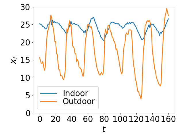
Figure 4: Example of a pair of indoor and outdoor temperature sequences.
Refer to caption
Figure 5: Color map representing the values of elements of estimated matrix cinvc_{\operatorname{inv}}.

7.3 Analysis of dynamical systems with RKHMs

Finally, we applied our method for extracting time-invariant relations in interacting dynamical systems by using real-world time-series data from a dataset with cause-effect pairs (Mooij et al. 2016). Two time-series data about indoor and outdoor temperatures (pairs0048) at time 0∼1600\sim 160 were used. The original sequences are shown in Figure 5. We can see that the indoor temperature becomes high 2∼52\sim 5 time steps after the outdoor one does. For the mathematical treatments mentioned in Section 6.1 , we added small noises to the original data by using random numbers generated by the Gaussian distribution with mean 00 and standard deviation 0.20.2. After that, we normalized the data so that the mean is 00 and the standard deviations is 11. We set xt=[yt,zt,yt+1,zt+1,…,yt+9,zt+9]∈ℝ20x_{t}=[y_{t},z_{t},y_{t+1},z_{t+1},\ldots,y_{t+9},z_{t+9}]\in\mathbb{R}^{20}, where yty_{t} and ztz_{t} are the indoor and outdoor temperatures at tt, respectively. Then, we computed the estimation of the Perron-Frobenius operator KK and the time invariant term cinvc_{\operatorname{inv}} in Eq. (7). In this case, m=20m=20, and we set TT as 150150.

The values of elements of matrix cinvc_{\operatorname{inv}} are shown in Figure 5. We also add figures in Appendix H. A point at (i,j)(i,j) represents the value of (i,j)(i,j)-element of cinvc_{\operatorname{inv}}. We can see the values of (2​i−1,2​j)(2i-1,2j) and (2​j,2​i−1)(2j,2i-1) for i=j+2∼j+5i=j+2\sim j+5 are large, which implies that yj+2∼yj+5y_{j+2}\sim y_{j+5} and ziz_{i} are similar.

8 Conclusions

In this paper, we proposed a new data analysis framework with RKHM. We showed the theoretical validity for constructing orthonormal systems in RKHMs. Then, we derived concrete procedures for orthonormalization in RKHMs, and applied those to generalize with RKHM kernel principal component analysis and the analysis of dynamical systems with Perron-Frobenius operators. This enables us to access and extract the rich information of structured data by introducing a positive definite kernel that describes similarities between all combinations of pairs of elements of data. Numerical results with synthetic and real-world data also show the advantage of our methods with RKHMs.

References

  • Álvarez et al. (2011) Álvarez, M., Rosasco, L., and Lawrence, N. Kernels for vector-valued functions: A review. Foundations and Trends in Machine Learning, 4, 06 2011. doi: 10.1561/2200000036.
  • Bakić & Guljaš (2001) Bakić, D. and Guljaš, B. Operators on Hilbert H∗H^{*}-modules. Journal of Operator Theory, 46:123–137, 2001.
  • Budišić et al. (2012) Budišić, M., Mohr, R., and Mezić, I. Applied Koopmanism. Chaos (Woodbury, N.Y.), 22:047510, 2012. doi: 10.1063/1.4772195.
  • Cnops (1992) Cnops, J. A Gram-Schmidt method in Hilbert modules. Clifford Algebras and their Applications in Mathematical Physics, 47:193–203, 1992.
  • Črnjarić-Žic et al. (2017) Črnjarić-Žic, N., Maćešić, S., and Mezić, I. Koopman operator spectrum for random dynamical systems. arXiv:1711.03146, 2017.
  • Frank & Manuilov (1995) Frank, M. and Manuilov, V. Diagonalizing ¡Ècompact¡É operators on Hilbert W∗W^{*}-modules. Zeitschrift für Analysis und ihre Anwendungen, 14:1–8, 1995.
  • Fujii & Kawahara (2019) Fujii, K. and Kawahara, Y. Dynamic mode decomposition in vector-valued reproducing kernel Hilbert spaces for extracting dynamical structure among observables. Neural Networks, 117:94–103, 2019. doi: https://doi.org/10.1016/j.neunet.2019.04.020.
  • Hashimoto et al. (2019) Hashimoto, Y., Ishikawa, I., Ikeda, M., Matsuo, Y., and Kawahara, Y. Krylov subspace method for nonlinear dynamical systems with random noise. arXiv:1909.03634v3, 2019.
  • Heo (2008) Heo, J. Reproducing kernel Hilbert C∗C^{*}-modules and kernels associated with cocycles. Journal of Mathematical Physics, 49(10):103507, 2008. doi: 10.1063/1.3000574.
  • Ishikawa et al. (2018) Ishikawa, I., Fujii, K., Ikeda, M., Hashimoto, Y., and Kawahara, Y. Metric on nonlinear dynamical systems with Perron-Frobenius operators. In Advances in Neural Information Processing Systems 31, pp. 2856–2866, 2018.
  • Itoh (1990) Itoh, S. Reproducing kernels in modules over C∗C^{*}-algebras and their applications. Journal of Mathematics in Nature Science, pp. 1–20, 1990.
  • Kadison (1983) Kadison, R. V. Diagonalizing matrices over operator algebras. Bulletin (New Series) of the American Mathematical Society, 8(1):84–86, 1983.
  • Kadri et al. (2016) Kadri, H., Duflos, E., Preux, P., Canu, S., Rakotomamonjy, A., and Audiffren, J. Operator-valued kernels for learning from functional response data. Journal of Machine Learning Research, 17(20):1–54, 2016.
  • Kawahara (2016) Kawahara, Y. Dynamic mode decomposition with reproducing kernels for Koopman spectral analysis. In Advances in Neural Information Processing Systems 29, pp. 911–919, 2016.
  • Klus et al. (2017) Klus, S., Schuster, I., and Muandet, K. Eigendecompositions of transfer operators in reproducing kernel Hilbert spaces. arXiv:1712.01572, 2017.
  • Klus et al. (2019) Klus, S., Nüske, F., Peitz, S., Niemann, J.-H., Clementi, C., and Schütte, C. Data-driven approximation of the Koopman generator: Model reduction, system identification, and control. arXiv:1909.10638, 2019.
  • Lance (1995) Lance, E. C. Hilbert C∗C^{*}-modules – a toolkit for operator algebraists, London Mathematical Society Lecture Note Series, vol. 210. Cambridge University Press,, England, 1995.
  • Landi & Pavlov (2009) Landi, G. and Pavlov, A. On orthogonal systems in Hilbert C∗C^{*}-modules. Journal of Operator Theory, 68, 06 2009.
  • Lim et al. (2015) Lim, N., d’Alché Buc, F., Auliac, C., and Michailidis, G. Operator-valued kernel-based vector autoregressive models for network inference. Machine Learning, 99(3):489–513, 2015. doi: 10.1007/s10994-014-5479-3.
  • Lusch et al. (2017) Lusch, B., Nathan Kutz, J., and Brunton, S. Deep learning for universal linear embeddings of nonlinear dynamics. Nature Communications, 9:4950, 12 2017. doi: 10.1038/s41467-018-07210-0.
  • Micchelli & Pontil (2005) Micchelli, C. A. and Pontil, M. On learning vector-valued functions. Neural Computation, 17(1):177–204, 2005. doi: 10.1162/0899766052530802.
  • Minh et al. (2016) Minh, H. Q., Bazzani, L., and Murino, V. A unifying framework in vector-valued reproducing kernel Hilbert spaces for manifold regularization and co-regularized multi-view learning. Journal of Machine Learning Research, 17(25):1–72, 2016.
  • Mooij et al. (2016) Mooij, J. M., Peters, J., Janzing, D., Zscheischler, J., and Schölkopf, B. Distinguishing cause from effect using observational data: Methods and benchmarks. Journal of Machine Learning Research, 17(32):1–102, 2016.
  • Saitoh & Sawano (2016) Saitoh, S. and Sawano, Y. Theory of reproducing kernels and applications. Springer Singapore, 2016. doi: 10.1007/978-981-10-0530-5.
  • Schölkopf & Smola (2001) Schölkopf, B. and Smola, A. J. Learning with kernels: Support vector machines, regularization, optimization, and beyond. MIT Press, Cambridge, MA, USA, 2001.
  • Takeishi et al. (2017a) Takeishi, N., Kawahara, Y., and Yairi, T. Subspace dynamic mode decomposition for stochastic Koopman analysis. Physical Review E, 96, 2017a. doi: 10.1103/PhysRevE.96.033310.
  • Takeishi et al. (2017b) Takeishi, N., Kawahara, Y., and Yairi, T. Learning Koopman invariant subspaces for dynamic mode decomposition. In Advances in Neural Information Processing Systems 30, pp. 1131–1141, 2017b.
  • Ye (2017) Ye, Y. The matrix Hilbert space and its application to matrix learning. arXiv:1706.08110v2, 2017.
  • Yun et al. (2012) Yun, K., Honorio, J., Chattopadhyay, D., Berg, T. L., and Samaras, D. Two-person interaction detection using body-pose features and multiple instance learning. In Computer Vision and Pattern Recognition Workshops (CVPRW), 2012.

We explain the notations used in this paper in Section A. Then, we briefly review existing methods in Sections B, C, E, and F and detailed statements and definitions about RKHMs with their proofs in Section D. In addition, we explain in detail the mathematical treatments for defining Perron-Frobenius operators discussed in Section 6.1 and show figures about the numerical results in Section H. Finally, we provide proofs of theorems, propositions, corollaries, and lemmas in Section I and pseudo-codes in Section J.

Appendix A Notations

In this section, we describe notations used in this paper. Small letters denote 𝒜\mathcal{A}-valued coefficients (often by a,b,c,da,b,c,d) or vectors in ℳ\mathcal{M} (often by p,q,u,v,wp,q,u,v,w). Small Greek letters denote ℂ\mathbb{C}-valued coefficients. Calligraphic capital letters denote sets. Bold capital letters denote finite dimentional 𝒜\mathcal{A}-linear map and bold small letters denote vectors in 𝒜n\mathcal{A}^{n} for n∈ℕn\in\mathbb{N} (a finite dimentional Hilbert C∗C^{*}-module). Small Roman letters denote vectors in ℂn\mathbb{C}^{n} (a finite dimensional vector space). Also, we use ∼\sim for objects related to RKHSs.

The typical notations in this paper are listed in Table 1 at the last page of this document.

Table 1: Notation table
ℂm×m\mathbb{C}^{m\times m} A set of all complex-valued m×mm\times m matrix
𝒜\mathcal{A} A C∗C^{*}-algebra
∥⋅∥𝒜\|\cdot\|_{\mathcal{A}} The norm in 𝒜\mathcal{A} (For 𝒜=ℂm×m\mathcal{A}=\mathbb{C}^{m\times m}, ‖c‖ℂm×m:=sup‖d‖2=1‖c​d‖2\|c\|_{\mathbb{C}^{m\times m}}:=\sup_{\|\mathrm{d}\|_{2}=1}\|c\mathrm{d}\|_{2})
ℳ\mathcal{M} A (right) 𝒜\mathcal{A}-module
|⋅||\cdot| The 𝒜\mathcal{A}-valued absolute value in ℳ\mathcal{M} defined as a positive element |u||u| such that |u|2=⟨u,u⟩|u|^{2}=\left\langle u,u\right\rangle
∥⋅∥\|\cdot\| The norm in ℳ\mathcal{M} defined as ‖u‖:=‖|⟨u,u⟩|‖𝒜\|u\|:=\||\left\langle u,u\right\rangle|\|_{\mathcal{A}}
𝒳\mathcal{X} A topological space
mm A natural number that represents the number of elements of data
nn, TT Natural numbers that represent the amount of observed data used for the estimation (TT for time-series data)
𝒴\mathcal{Y} A set of observed data 𝒴:={x0,x1,…}⊆𝒳m\mathcal{Y}:=\{x_{0},x_{1},\ldots\}\subseteq\mathcal{X}^{m} (a countable and dense subset of 𝒳m\mathcal{X}^{m} whose elements are completely different)
kk An 𝒜\mathcal{A}-valued positive definite kernel
ϕ\phi The feature map endowed with kk
ℳk\mathcal{M}_{k} The RKHM associated with kk
𝒜𝒴\mathcal{A}^{\mathcal{Y}} The set of all functions from 𝒴\mathcal{Y} to 𝒜\mathcal{A}
|⋅|k|\cdot|_{k} The 𝒜\mathcal{A}-valued absolute value in ℳk\mathcal{M}_{k}
∥⋅∥k\|\cdot\|_{k} The norm in ℳk\mathcal{M}_{k}
k~\tilde{k} A complex-valued positive definite kernel
ϕ~\tilde{\phi} The feature map endowed with k~\tilde{k}
ℋk~\mathcal{H}_{\tilde{k}} The RKHS associated with k~\tilde{k}
ϵ\epsilon The parameter that determines the theoretical accuracy and numerical stability
WW The linear operator from 𝒜n\mathcal{A}^{n} to ℳk\mathcal{M}_{k} composed of observed data ϕ⁡(x1),…,ϕ⁡(xn)\phi(x_{1}),\ldots,\phi(x_{n})
𝐆\mathbf{G} A Gram matrix
{qt}t=1∞\{q_{t}\}_{t=1}^{\infty} An orthonormal system in ℳ\mathcal{M} or ℳk\mathcal{M}_{k}
QQ The linear operator from 𝒜n\mathcal{A}^{n} to ℳk\mathcal{M}_{k} composed of q1,…,qnq_{1},\ldots,q_{n}
𝐑\mathbf{R} The n×nn\times n 𝒜\mathcal{A}-valued matrix that satisfies ‖W−Q​𝐑‖≤ϵ\|W-Q\mathbf{R}\|\leq\epsilon
𝐑inv\mathbf{R}_{\operatorname{inv}} The n×nn\times n 𝒜\mathcal{A}-valued matrix that satisfies Q=W​𝐑invQ=W\mathbf{R}_{\operatorname{inv}}
psp_{s} The ss-th principal axis generated by kernel PCA with an RKHM
KK A Perron-Frobenius operator on ℳk\mathcal{M}_{k}
𝐊T\mathbf{K}_{T} The estimation of KK with observed data {x0,…,xT−1}\{x_{0},\ldots,x_{T-1}\}
a^T,S\hat{a}_{T,S} The abnormality at SS computed with 𝐊T\mathbf{K}_{T}

Appendix B RKHS

In this section, we review the theory of RKHSs. RKHSs are Hilbert spaces to extract nonlinearity or higher-order moments of data (Schölkopf & Smola 2001; Saitoh & Sawano 2016).

We begin with a positive difinite kernel. Let 𝒴\mathcal{Y} be a non-empty set for data, and k~\tilde{k} be a positive definite kernel, which is defined as follows:

Definition B.1.

A map k~:𝒴×𝒴→ℂ\tilde{k}:\mathcal{Y}\times\mathcal{Y}\to\mathbb{C} is called a positive definite kernel if it satisfies the following conditions:

1. k~​(x,y)=k~​(y,x)¯\tilde{k}(x,y)=\overline{\tilde{k}(y,x)}  for x,y∈𝒴x,y\in\mathcal{Y}
2. ∑s,t=1ncs¯​ct​k~​(xs,xt)≥0\sum_{s,t=1}^{n}\overline{c_{s}}c_{t}\tilde{k}(x_{s},x_{t})\geq 0  for n∈ℕn\in\mathbb{N}, c1,…,cn∈ℂc_{1},\ldots,c_{n}\in\mathbb{C}, x1,…,xn∈𝒴x_{1},\ldots,x_{n}\in\mathcal{Y}.

Let ϕ~:𝒴→ℂ𝒴\tilde{\phi}:\mathcal{Y}\to\mathbb{C}^{\mathcal{Y}} be a map defined as ϕ~​(x)=k~​(⋅,x)\tilde{\phi}(x)=\tilde{k}(\cdot,x). With ϕ~\tilde{\phi}, the following space as the subset of ℂ𝒴\mathbb{C}^{\mathcal{Y}} is constructed:

ℋk~,0:={∑t=1nctϕ~(xt)|n∈ℕ,ct∈ℂ,xt∈𝒴}.\mathcal{H}_{\tilde{k},0}:=\bigg\{\sum_{t=1}^{n}c_{t}\tilde{\phi}(x_{t})\bigg|\ n\in\mathbb{N},\ c_{t}\in\mathbb{C},\ x_{t}\in\mathcal{Y}\bigg\}.

Then, a map ⟨⋅,⋅⟩k~:ℋk~,0×ℋk~,0→ℂ\left\langle\cdot,\cdot\right\rangle_{\tilde{k}}:\mathcal{H}_{\tilde{k},0}\times\mathcal{H}_{\tilde{k},0}\to\mathbb{C} is defined as follows:

⟨∑s=1ncs​ϕ~​(xs),∑t=1ldt​ϕ~​(yt)⟩k~:=∑s=1n∑t=1lcs¯​dt​k~​(xs,yt).\bigg\langle\sum_{s=1}^{n}c_{s}\tilde{\phi}(x_{s}),\sum_{t=1}^{l}d_{t}\tilde{\phi}(y_{t})\bigg\rangle_{\tilde{k}}:=\sum_{s=1}^{n}\sum_{t=1}^{l}\overline{c_{s}}d_{t}\tilde{k}(x_{s},y_{t}).

By the properties in Definition B.1 of k~\tilde{k}, ⟨⋅,⋅⟩k~\left\langle\cdot,\cdot\right\rangle_{\tilde{k}} is well-defined, satisfies the axiom of inner products, and has the reproducing property, that is,

⟨ϕ~​(x),v⟩k~=v⁡(x),\langle\tilde{\phi}(x),v\rangle_{\tilde{k}}=v(x),

for v∈ℋk~,0v\in\mathcal{H}_{\tilde{k},0} and x∈𝒴x\in\mathcal{Y}.

The completion of ℋk~,0\mathcal{H}_{\tilde{k},0} is called RKHS associated with k~\tilde{k} and denoted as ℋk~\mathcal{H}_{\tilde{k}}. It can be shown that ⟨⋅,⋅⟩k~\left\langle\cdot,\cdot\right\rangle_{\tilde{k}} is extended continuously to ℋk~\mathcal{H}_{\tilde{k}} and the map ℋk~∋v↦(x↦⟨ϕ~​(x),v⟩k~)∈ℂ𝒴\mathcal{H}_{\tilde{k}}\ni v\mapsto(x\mapsto\langle\tilde{\phi}(x),v\rangle_{\tilde{k}})\in\mathbb{C}^{\mathcal{Y}} is injective. Thus, ℋk~\mathcal{H}_{\tilde{k}} is regarded to be the subset of ℂ𝒴\mathbb{C}^{\mathcal{Y}} and has the reproducing property. Also, by the Moore-Aronszajn theorem, ℋk~\mathcal{H}_{\tilde{k}} is determined uniquely.

ϕ~\tilde{\phi} maps data into ℋk~\mathcal{H}_{\tilde{k}}, whose dimension is generally higher (often infinite dimensional) than that of 𝒴\mathcal{Y}, and is called the feature map. Since the dimension of ℋk~\mathcal{H}_{\tilde{k}} is higher than that of 𝒴\mathcal{Y}, complicated behaviors of data in 𝒴\mathcal{Y} are often transformed into simple ones in ℋk~\mathcal{H}_{\tilde{k}} (Schölkopf & Smola 2001).

Appendix C vv-RKHS

In this section, we review the theory of vv-RKHSs.

Similar to the case of RKHSs, we begin with a positive definite kernel. Let 𝒴\mathcal{Y} be a non-empty set for data, 𝒲\mathcal{W} be a Hilbert space equipped with an inner product ⟨⋅,⋅⟩𝒲\left\langle\cdot,\cdot\right\rangle_{\mathcal{W}}, and ℒ⁡(𝒲)\mathcal{L}(\mathcal{W}) be the space of bounded linear operators on 𝒲\mathcal{W}. In addition, kk be an operator valued positive definite kernel, which is defined as follows:

Definition C.1.

A map map k:𝒴×𝒴→ℒ⁡(𝒲)k:\mathcal{Y}\times\mathcal{Y}\to\mathcal{L}(\mathcal{W}) is called an operator valued positive definite kernel if it satisfies the following conditions:

1. k⁡(x,y)=k​(y,x)∗k(x,y)=k(y,x)^{*}  for x,y∈𝒴x,y\in\mathcal{Y}
2. ∑s,t=1n⟨vs,k⁡(xs,xt)​vt⟩𝒲≥0\sum_{s,t=1}^{n}\left\langle v_{s},k(x_{s},x_{t})v_{t}\right\rangle_{\mathcal{W}}\geq 0  for n∈ℕn\in\mathbb{N}, v1,…,vn∈𝒲v_{1},\ldots,v_{n}\in\mathcal{W}, x1,…,xn∈𝒴x_{1},\ldots,x_{n}\in\mathcal{Y}.

For v∈𝒲v\in\mathcal{W}, let ϕv:𝒴→𝒲𝒴\phi_{v}:\mathcal{Y}\to\mathcal{W}^{\mathcal{Y}} be a map defined as ϕv​(x)=k⁡(⋅,x)​v\phi_{v}(x)=k(\cdot,x)v. With ϕ\phi, the following space as the subset of 𝒲𝒴\mathcal{W}^{\mathcal{Y}} is constructed:

ℋk,0v:={∑t=0nϕvt(xt)|n∈ℕ,vt∈𝒲,xt∈𝒴,}.\mathcal{H}_{k,0}^{\operatorname{v}}:=\bigg\{\sum_{t=0}^{n}\phi_{v_{t}}(x_{t})\bigg|n\in\mathbb{N},\ v_{t}\in\mathcal{W},\ x_{t}\in\mathcal{Y},\bigg\}.

Then, a map ⟨⋅,⋅⟩k,v:ℋk,0v×ℋk,0v→ℂ\left\langle\cdot,\cdot\right\rangle_{k,{\operatorname{v}}}:\mathcal{H}_{k,0}^{\operatorname{v}}\times\mathcal{H}_{k,0}^{\operatorname{v}}\to\mathbb{C} is defined as follows:

⟨∑s=1nϕvt​(xt),∑t=0lϕwt​(yt)⟩k,v\displaystyle\bigg\langle\sum_{s=1}^{n}\phi_{v_{t}}(x_{t}),\sum_{t=0}^{l}\phi_{w_{t}}(y_{t})\bigg\rangle_{k,{\operatorname{v}}}
:=∑s=1n∑t=1l⟨vs,k⁡(xs,yt)​wt⟩𝒲.\displaystyle\qquad:=\sum_{s=1}^{n}\sum_{t=1}^{l}\left\langle v_{s},k(x_{s},y_{t})w_{t}\right\rangle_{\mathcal{W}}.

By the properties in Definition C.1 of kk, ⟨⋅,⋅⟩k,v\left\langle\cdot,\cdot\right\rangle_{k,{\operatorname{v}}} is well-defined, satisfies the axiom of inner products and has the reproducing property, that is,

⟨ϕv​(x),u⟩k,v=⟨v,u⁡(x)⟩𝒲,\left\langle\phi_{v}(x),u\right\rangle_{k,{\operatorname{v}}}=\left\langle v,u(x)\right\rangle_{\mathcal{W}},

for u∈ℋk,0vu\in\mathcal{H}_{k,0}^{{\operatorname{v}}} and x∈𝒴x\in\mathcal{Y}.

The completion of ℋk,0v\mathcal{H}_{k,0}^{\operatorname{v}} is called vv-RKHS associated with kk and denoted as ℋk,v\mathcal{H}_{k,{\operatorname{v}}}. Note that since the inner product in ℋkv\mathcal{H}_{k}^{\operatorname{v}} is defined with the complex-valued inner product in 𝒲\mathcal{W}, it is complex-valued.

Appendix D Statements and definitions about RKHMs and their proofs

In this section, we provide the precise statements and definitions about RKHMs introduced in Section 2 and show their proofs.

Definition D.1 (C∗C^{*}-algebra).

A set 𝒜\mathcal{A} is called a C∗C^{*}-algebra if it satisfies the following conditions:

1. 𝒜\mathcal{A} is an algebra over ℂ\mathbb{C}, and there exists a bijection (⋅)∗:𝒜→𝒜(\cdot)^{*}:\mathcal{A}\to\mathcal{A} that satisfies the following conditions for λ,μ∈ℂ\lambda,\mu\in\mathbb{C} and c,d∈𝒜c,d\in\mathcal{A}:

∙\bullet (λ​c+μ​d)∗=λ¯​c∗+μ¯​d∗(\lambda c+\mu d)^{*}=\overline{\lambda}c^{*}+\overline{\mu}d^{*}
∙\bullet (c​d)∗=d∗​c∗(cd)^{*}=d^{*}c^{*}
∙\bullet (c∗)∗=c(c^{*})^{*}=c

2. 𝒜\mathcal{A} is a norm space with ∥⋅∥𝒜\|\cdot\|_{\mathcal{A}}, and for c,d∈𝒜c,d\in\mathcal{A}, ‖c​d‖𝒜≤‖c‖𝒜​‖d‖𝒜\|cd\|_{\mathcal{A}}\leq\|c\|_{\mathcal{A}}\|d\|_{\mathcal{A}} holds. In addition, 𝒜\mathcal{A} is complete with respect to ∥⋅∥𝒜\|\cdot\|_{\mathcal{A}}.

3. For c∈𝒜c\in\mathcal{A}, ‖c∗​c‖𝒜=‖c‖𝒜2\|c^{*}c\|_{\mathcal{A}}=\|c\|_{\mathcal{A}}^{2} holds.

Definition D.2 (Positive).

c∈𝒜c\in\mathcal{A} is called positive if there exists d∈𝒜d\in\mathcal{A} such that c=d∗​dc=d^{*}d holds. For a positive element c∈𝒜c\in\mathcal{A}, we denote c≥0c\geq 0.

Definition D.3 ((Right) multiplication).

Let ℳ\mathcal{M} be an abelian group with operation ++. For c,d∈𝒜c,d\in\mathcal{A} and u,v∈ℳu,v\in\mathcal{M}, if an operation ⋅:ℳ×𝒜→ℳ\cdot:\mathcal{M}\times\mathcal{A}\to\mathcal{M} satisfies

1. (u+v)⋅c=u⋅c+v⋅c(u+v)\cdot c=u\cdot c+v\cdot c
2. u⋅(c+d)=u⋅c+u⋅du\cdot(c+d)=u\cdot c+u\cdot d
3. u⋅(c​d)=(u⋅d)⋅cu\cdot(cd)=(u\cdot d)\cdot c
4. u⋅1𝒜=uu\cdot 1_{\mathcal{A}}=u,

where 1𝒜1_{\mathcal{A}} is the multiplicative identity of 𝒜\mathcal{A}, then, ⋅\cdot is called (right) 𝒜\mathcal{A}-multiplication. The multiplication u⋅cu\cdot c is usually denoted as u​cuc.

Remark D.4.

For practical applications of the theory of RKHSs, considering column vectors rather than row vectors is standard for representing coefficients. Column vectors act on the right. Therefore, we consider right multiplications for making algorithms with RKHMs (with 𝒜\mathcal{A}-multiplications) compatible with those with RKHSs.

Definition D.5 (C∗C^{*}-module).

Let ℳ\mathcal{M} be an abelian group with operation ++. If ℳ\mathcal{M} has the structure of a (right) 𝒜\mathcal{A}-multiplication, ℳ\mathcal{M} is called a (right) C∗C^{*}-module over 𝒜\mathcal{A}.

Definition D.6 (Hilbert C∗C^{*}-module).

Let ℳ\mathcal{M} be a (right) C∗C^{*}-module over 𝒜\mathcal{A} which is equipped with an 𝒜\mathcal{A}-valued inner product defined in Definition 2.1. If ℳ\mathcal{M} is complete with respect to the norm ∥⋅∥\|\cdot\|, it is called a Hilbert C∗C^{*}-module over 𝒜\mathcal{A}.

Lemma D.7 (Cauchy-Schwarz inequality (Lance 1995)).

For u,v∈ℳu,v\in\mathcal{M}, the following inequality holds:

|⟨u,v⟩|2≤‖u‖2​⟨v,v⟩.|\left\langle u,v\right\rangle|^{2}\leq\|u\|^{2}\left\langle v,v\right\rangle.
Remark D.8.

The proof of Cauchy-Shwarz inequality only requires properties 1 and 2 about 𝒜\mathcal{A}-valued inner products in Definition 2.1.

Lemma D.9.

Let 𝒲\mathcal{W} be a Hilbert space equipped with an inner product ⟨⋅,⋅⟩𝒲\left\langle\cdot,\cdot\right\rangle_{\mathcal{W}}, and ℒ⁡(𝒲)\mathcal{L}(\mathcal{W}) be the space of bounded linear operators on 𝒲\mathcal{W}. If 𝒜=ℒ⁡(𝒲)\mathcal{A}=\mathcal{L}(\mathcal{W}), then, the 𝒜\mathcal{A}-valued positive definite kernel defined in Definition 2.2 is equivalent to the operator valued positive definite kernel defined in Definition C.1.

Proof.

Let kk be an 𝒜\mathcal{A}-valued positive definite kernel defined in Definition 2.2. Let v∈𝒲v\in\mathcal{W}. For n∈ℕn\in\mathbb{N}, v1,…,vn∈𝒲v_{1},\ldots,v_{n}\in\mathcal{W}, let ct∈ℒ⁡(𝒲)c_{t}\in\mathcal{L}(\mathcal{W}) be defined as ct​u:=⟨v,u⟩𝒲/⟨v,v⟩𝒲​vtc_{t}u:=\left\langle v,u\right\rangle_{\mathcal{W}}/\left\langle v,v\right\rangle_{\mathcal{W}}v_{t} for u∈𝒲u\in\mathcal{W}. Since vt=ct​vv_{t}=c_{t}v holds, the following equalities are derived for x1,…,xn∈𝒴x_{1},\ldots,x_{n}\in\mathcal{Y}:

∑s,t=1n⟨vt,k⁡(xt,xs)​vs⟩𝒲\displaystyle\sum_{s,t=1}^{n}\left\langle v_{t},k(x_{t},x_{s})v_{s}\right\rangle_{\mathcal{W}} =∑s,t=1n⟨ct​v,k⁡(xt,xs)​cs​v⟩𝒲\displaystyle=\sum_{s,t=1}^{n}\left\langle c_{t}v,k(x_{t},x_{s})c_{s}v\right\rangle_{\mathcal{W}}
=⟨v,∑s,t=1nct∗​k​(xt,xs)​cs​v⟩𝒲.\displaystyle=\bigg\langle v,\sum_{s,t=1}^{n}c_{t}^{*}k(x_{t},x_{s})c_{s}v\bigg\rangle_{\mathcal{W}}.

By the positivity of ∑s,t=1nct∗​k​(xt,xs)​cs\sum_{s,t=1}^{n}c_{t}^{*}k(x_{t},x_{s})c_{s}, ⟨v,∑s,t=1nct∗​k​(xt,xs)​cs​v⟩𝒲≥0\langle v,\sum_{s,t=1}^{n}c_{t}^{*}k(x_{t},x_{s})c_{s}v\rangle_{\mathcal{W}}\geq 0 holds, which implies kk is an operator valued positive definite kernel defined in Definition C.1.

On the other hand, let kk be an operator valued positive definite kernel defined in Definition C.1. Let v∈𝒲v\in\mathcal{W}. For n∈ℕn\in\mathbb{N}, c1,…,cn∈𝒜c_{1},\ldots,c_{n}\in\mathcal{A} and x1,…,xn∈𝒴x_{1},\ldots,x_{n}\in\mathcal{Y}, the following equality is derived:

⟨v,∑s,t=1nct∗​k​(xt,xs)​cs​v⟩𝒲=∑s,t=1n⟨ct​v,k⁡(xt,xs)​cs​v⟩𝒲.\displaystyle\bigg\langle v,\sum_{s,t=1}^{n}c_{t}^{*}k(x_{t},x_{s})c_{s}v\bigg\rangle_{\mathcal{W}}\!\!\!\!=\sum_{s,t=1}^{n}\left\langle c_{t}v,k(x_{t},x_{s})c_{s}v\right\rangle_{\mathcal{W}}.

By Definition C.1, ∑s,t=1n⟨ct​v,k⁡(xt,xs)​cs​v⟩𝒲≥0\sum_{s,t=1}^{n}\left\langle c_{t}v,k(x_{t},x_{s})c_{s}v\right\rangle_{\mathcal{W}}\geq 0 holds, which implies kk is an 𝒜\mathcal{A}-valued positive definite kernel defined in Definition 2.2. ∎

Proposition D.10.

⟨⋅,⋅⟩k\left\langle\cdot,\cdot\right\rangle_{k} is an 𝒜\mathcal{A}-valued inner product.

Proof.

Property 1 in Definition 2.1 is followed by the definition of ⟨⋅,⋅⟩k\left\langle\cdot,\cdot\right\rangle_{k}. The following equality for v:=∑t=0nϕ⁡(xt)​ctv:=\sum_{t=0}^{n}\phi(x_{t})c_{t} and w:=∑s=0lϕ⁡(ys)​dsw:=\sum_{s=0}^{l}\phi(y_{s})d_{s} implies ⟨⋅,⋅⟩k\left\langle\cdot,\cdot\right\rangle_{k} satisfies property 2:

⟨v,w⟩k\displaystyle\left\langle v,w\right\rangle_{k} =⟨∑t=0nϕ⁡(xt)​ct,∑s=0lϕ⁡(ys)​ds⟩k\displaystyle=\bigg\langle\sum_{t=0}^{n}\phi(x_{t})c_{t},\sum_{s=0}^{l}\phi(y_{s})d_{s}\bigg\rangle_{k}
=∑t=0n∑s=1lct∗​k​(xt,ys)​ds\displaystyle=\sum_{t=0}^{n}\sum_{s=1}^{l}c_{t}^{*}k(x_{t},y_{s})d_{s}
=(∑t=0n∑s=0lds∗​k​(ys,xt)​ct)∗\displaystyle=\bigg(\sum_{t=0}^{n}\sum_{s=0}^{l}d_{s}^{*}k(y_{s},x_{t})c_{t}\bigg)^{*}
=⟨∑s=0lϕ⁡(ys)​ds,∑t=0nϕ⁡(xt)​ct⟩k∗\displaystyle=\bigg\langle\sum_{s=0}^{l}\phi(y_{s})d_{s},\sum_{t=0}^{n}\phi(x_{t})c_{t}\bigg\rangle_{k}^{*}
=⟨w,v⟩k∗.\displaystyle=\left\langle w,v\right\rangle_{k}^{*}.

Concerning property 3, ⟨u,u⟩k≥0\left\langle u,u\right\rangle_{k}\geq 0 for u∈ℳku\in\mathcal{M}_{k} holds by the positive definiteness of kk (Definition 2.2.2). In addition, by Cauchy-Schwarz inequality (Lemma D.7 and Remark D.8), the following inequality holds for x∈𝒴x\in\mathcal{Y}:

|v⁡(x)|𝒜2=|⟨ϕ⁡(x),v⟩k|𝒜2≤‖k⁡(x,x)‖𝒜​⟨v,v⟩k.|v(x)|^{2}_{\mathcal{A}}=|\left\langle\phi(x),v\right\rangle_{k}|^{2}_{\mathcal{A}}\leq\|k(x,x)\|_{\mathcal{A}}\left\langle v,v\right\rangle_{k}.

Thus, if ⟨v,v⟩k=0\left\langle v,v\right\rangle_{k}=0, then |v⁡(x)|𝒜=0|v(x)|_{\mathcal{A}}=0 for all x∈𝒴x\in\mathcal{Y}, which implies v=0v=0. ∎

Proposition D.11.

⟨⋅,⋅⟩k\left\langle\cdot,\cdot\right\rangle_{k} is extended continuously to ℳk\mathcal{M}_{k} and the map ℳk∋v↦(x↦⟨ϕ⁡(x),v⟩k)∈𝒜𝒴\mathcal{M}_{k}\ni v\mapsto(x\mapsto\left\langle\phi(x),v\right\rangle_{k})\in\mathcal{A}^{\mathcal{Y}} is injective. Thus, ℳk\mathcal{M}_{k} is regarded to be the subset of 𝒜𝒴\mathcal{A}^{\mathcal{Y}} and has the reproducing property.

Proof.

(Existence) For v,w∈ℳkv,w\in\mathcal{M}_{k}, there exist vt,wt∈ℳk,0​(t=1,2,…)v_{t},w_{t}\in\mathcal{M}_{k,0}\ (t=1,2,\ldots) such that v=limt→∞vtv=\lim_{t\to\infty}v_{t} and w=limt→∞wtw=\lim_{t\to\infty}w_{t}. By Cauchy-Schwarz inequality (Lemma D.7), the following inequalities hold:

‖⟨vt,wt⟩k−⟨vs,ws⟩k‖𝒜\displaystyle\|\left\langle v_{t},w_{t}\right\rangle_{k}-\left\langle v_{s},w_{s}\right\rangle_{k}\|_{\mathcal{A}}
≤‖⟨vt,wt−ws⟩k‖𝒜+‖⟨vt−vs,ws⟩k‖𝒜\displaystyle\quad\leq\|\left\langle v_{t},w_{t}-w_{s}\right\rangle_{k}\|_{\mathcal{A}}+\|\left\langle v_{t}-v_{s},w_{s}\right\rangle_{k}\|_{\mathcal{A}}
≤‖vt‖k​‖wt−ws‖k+‖vt−vs‖k​‖ws‖k\displaystyle\quad\leq\|v_{t}\|_{k}\|w_{t}-w_{s}\|_{k}+\|v_{t}-v_{s}\|_{k}\|w_{s}\|_{k}
→0(t,s→∞),\displaystyle\quad\to 0\ (t,s\to\infty),

which implies {⟨vt,wt⟩k}t=1∞\{\left\langle v_{t},w_{t}\right\rangle_{k}\}_{t=1}^{\infty} is a Cauchy sequence in 𝒜\mathcal{A}. By the completeness of 𝒜\mathcal{A}, there exists a limit limt→∞⟨vt,wt⟩k\lim_{t\to\infty}\left\langle v_{t},w_{t}\right\rangle_{k}.

(Well-definedness) Assume there exist vt′,wt′∈ℳk,0​(t=1,2,…)v^{\prime}_{t},w^{\prime}_{t}\in\mathcal{M}_{k,0}\ (t=1,2,\ldots) such that v=limt→∞vt=limt→∞vt′v=\lim_{t\to\infty}v_{t}=\lim_{t\to\infty}v^{\prime}_{t} and w=limt→∞wt=limt→∞wt′w=\lim_{t\to\infty}w_{t}=\lim_{t\to\infty}w^{\prime}_{t}. By Cauchy-Schwarz inequality (Lemma D.7), ‖⟨vt,wt⟩k−⟨vt′,wt′⟩k‖𝒜≤‖vt‖k​‖wt−wt′‖k+‖vt−vt′‖k​‖wt′‖k→0​(t→∞)\|\left\langle v_{t},w_{t}\right\rangle_{k}-\left\langle v^{\prime}_{t},w^{\prime}_{t}\right\rangle_{k}\|_{\mathcal{A}}\leq\|v_{t}\|_{k}\|w_{t}-w^{\prime}_{t}\|_{k}+\|v_{t}-v^{\prime}_{t}\|_{k}\|w^{\prime}_{t}\|_{k}\to 0\ (t\to\infty) holds, which implies limt→∞⟨vt,wt⟩k=limt→∞⟨vt′,wt′⟩k\lim_{t\to\infty}\left\langle v_{t},w_{t}\right\rangle_{k}=\lim_{t\to\infty}\left\langle v^{\prime}_{t},w^{\prime}_{t}\right\rangle_{k}.

(Injectivity) For v,w∈ℳkv,w\in\mathcal{M}_{k}, we assume ⟨ϕ⁡(x),v⟩k=⟨ϕ⁡(x),w⟩k\left\langle\phi(x),v\right\rangle_{k}=\left\langle\phi(x),w\right\rangle_{k} for x∈𝒴x\in\mathcal{Y}. By the linearity of ⟨⋅,⋅⟩k\left\langle\cdot,\cdot\right\rangle_{k}, ⟨u,v⟩k=⟨u,v⟩k\left\langle u,v\right\rangle_{k}=\left\langle u,v\right\rangle_{k} holds for u∈ℳk,0u\in\mathcal{M}_{k,0}. For u∈ℳku\in\mathcal{M}_{k}, there exist ut∈ℳk,0​(t=1,2,…)u_{t}\in\mathcal{M}_{k,0}\ (t=1,2,\ldots) such that u=limt→∞utu=\lim_{t\to\infty}u_{t}. Therefore, ⟨u,v−w⟩k=limt→∞⟨ut,v−w⟩k=0\left\langle u,v-w\right\rangle_{k}=\lim_{t\to\infty}\left\langle u_{t},v-w\right\rangle_{k}=0. As a result, ⟨v−w,v−w⟩k=0\left\langle v-w,v-w\right\rangle_{k}=0 holds by setting u=v−wu=v-w, which implies v=wv=w. ∎

Proposition D.12.

Assume a Hilbert C∗C^{*}-module ℳ\mathcal{M} over 𝒜\mathcal{A} and a map ψ:𝒴→ℳ\psi:\mathcal{Y}\to\mathcal{M} satisfy the following conditions:

1. ∀x,y∈𝒴{}^{\forall}x,y\in\mathcal{Y}, ⟨ψ⁡(x),ψ⁡(y)⟩ℳ=k⁡(x,y)\left\langle\psi(x),\psi(y)\right\rangle_{\mathcal{M}}=k(x,y)

2. {∑t=0nψ(xt)ct∣xt∈𝒴,ct∈𝒜}¯=ℳ\overline{\{\sum_{t=0}^{n}\psi(x_{t})c_{t}\mid\ x_{t}\in\mathcal{Y},\ c_{t}\in\mathcal{A}\}}=\mathcal{M}

Then, there exists a unique 𝒜\mathcal{A}-linear bijection map Ψ:ℳk→ℳ\Psi:\mathcal{M}_{k}\to\mathcal{M} that preserves the inner product and satisfies the following commutative diagram:

ℳk\textstyle{\mathcal{M}_{k}\ignorespaces\ignorespaces\ignorespaces\ignorespaces}Ψ\scriptstyle{\Psi}ℳ\textstyle{\mathcal{M}}𝒴\textstyle{\mathcal{Y}\ignorespaces\ignorespaces\ignorespaces\ignorespaces\ignorespaces\ignorespaces\ignorespaces\ignorespaces\ignorespaces\ignorespaces\ignorespaces\ignorespaces\ignorespaces}ϕ\scriptstyle{\phi}ψ\scriptstyle{\psi}↻\scriptstyle{\circlearrowright} (10)
Proof.

We define Ψ:ℳk,0→ℳ\Psi:\mathcal{M}_{k,0}\to\mathcal{M} as an 𝒜\mathcal{A}-linear map that satisfies Ψ⁡(ϕ⁡(x))=ψ⁡(x)\Psi(\phi(x))=\psi(x). We show Ψ\Psi can be extended to a unique 𝒜\mathcal{A}-linear bijection map on ℳk\mathcal{M}_{k} , which preserves the inner product.

(Uniqueness) The uniqueness follows by the definition of Ψ\Psi.

(Inner product preservation) For x,y∈𝒴x,y\in\mathcal{Y}, equalities ⟨Ψ⁡(ϕ⁡(x)),Ψ⁡(ϕ⁡(y))⟩k=⟨ψ⁡(x),ψ⁡(y)⟩ℳ=k⁡(x,y)=⟨ϕ⁡(x),ϕ⁡(y)⟩k\left\langle\Psi(\phi(x)),\Psi(\phi(y))\right\rangle_{k}=\left\langle\psi(x),\psi(y)\right\rangle_{\mathcal{M}}=k(x,y)=\left\langle\phi(x),\phi(y)\right\rangle_{k} hold. Since Ψ\Psi is 𝒜\mathcal{A}-linear, Ψ\Psi preserves the inner products between arbitrary u,v∈ℳk,0u,v\in\mathcal{M}_{k,0}

(Well-definedness) Since Φ\Phi preserves the inner product, if {vt}t=1∞⊆ℳk\{v_{t}\}_{t=1}^{\infty}\subseteq\mathcal{M}_{k} is a Cauchy sequence, {Ψ⁡(vt)}t=1∞⊆ℳ\{\Psi(v_{t})\}_{t=1}^{\infty}\subseteq\mathcal{M} is also a Cauchy sequence. Therefore, by the completeness of ℳ\mathcal{M}, Ψ\Psi also preserves the inner product in ℳk\mathcal{M}_{k}, and for v∈ℳkv\in\mathcal{M}_{k}, ‖Ψ⁡(v)‖ℳ=‖v‖k\|\Psi(v)\|_{\mathcal{M}}=\|v\|_{k} holds. As a result, for v∈ℳkv\in\mathcal{M}_{k}, if v=0v=0, ‖Ψ⁡(v)‖ℳ=‖v‖k=0\|\Psi(v)\|_{\mathcal{M}}=\|v\|_{k}=0 holds. This implies Ψ⁡(v)=0\Psi(v)=0.

(Injectivity) For v,w∈ℳkv,w\in\mathcal{M}_{k}, if Ψ⁡(v)=Ψ⁡(w)\Psi(v)=\Psi(w), then 0=‖Ψ⁡(v)−Ψ⁡(w)‖ℳ=‖v−w‖k0=\|\Psi(v)-\Psi(w)\|_{\mathcal{M}}=\|v-w\|_{k} holds since Ψ\Psi preserves the inner product, which implies v=wv=w.

(Surjectivity) The surjectivity follows directly by the condition {∑t=0nψ(xt)ct∣xt∈𝒴,ct∈𝒜}¯=ℳ\overline{\{\sum_{t=0}^{n}\psi(x_{t})c_{t}\mid\ x_{t}\in\mathcal{Y},\ c_{t}\in\mathcal{A}\}}=\mathcal{M}. ∎

Lemma D.13.

𝒜n\mathcal{A}^{n} is a Hilbert C∗C^{*}-module equipped with an 𝒜\mathcal{A}-valued inner product ⟨⋅,⋅⟩𝒜n\left\langle\cdot,\cdot\right\rangle_{\mathcal{A}^{n}} defined as ⟨𝐮,𝐯⟩𝒜n:=∑t=1nut∗​vt\left\langle\mathbf{u},\mathbf{v}\right\rangle_{\mathcal{A}^{n}}:=\sum_{t=1}^{n}u_{t}^{*}v_{t} for 𝐮=[u1,…,un],𝐯=[v1,…,vn]∈𝒜n\mathbf{u}=[u_{1},\ldots,u_{n}],\mathbf{v}=[v_{1},\ldots,v_{n}]\in\mathcal{A}^{n} where u1,…,un,v1,…,vn∈𝒜u_{1},\ldots,u_{n},v_{1},\ldots,v_{n}\in\mathcal{A}.

Proof.

Let k:𝒜n×𝒜n→𝒜k:\mathcal{A}^{n}\times\mathcal{A}^{n}\to\mathcal{A} be a map defined by k⁡(𝐮,𝐯)=∑t=1nut∗​vtk(\mathbf{u},\mathbf{v})=\sum_{t=1}^{n}u_{t}^{*}v_{t} for 𝐮=[u1,…,un],𝐯=[v1,…,vn]∈𝒜n\mathbf{u}=[u_{1},\ldots,u_{n}],\mathbf{v}=[v_{1},\ldots,v_{n}]\in\mathcal{A}^{n}. Then, k⁡(𝐮,𝐯)=k​(𝐯,𝐮)∗k(\mathbf{u},\mathbf{v})=k(\mathbf{v},\mathbf{u})^{*} holds, and the following equalities hold for n∈ℕn\in\mathbb{N}, c1,…,cn∈𝒜c_{1},\ldots,c_{n}\in\mathcal{A} and 𝐮1,…,𝐮n∈𝒜n\mathbf{u}_{1},\ldots,\mathbf{u}_{n}\in\mathcal{A}^{n}:

∑s,t=1ncs∗​k​(𝐮s,𝐮t)​ct\displaystyle\sum_{s,t=1}^{n}c_{s}^{*}k(\mathbf{u}_{s},\mathbf{u}_{t})c_{t} =∑s,t=1ncs∗​∑j=1m𝐮s,j∗​𝐮t,j​ct\displaystyle=\sum_{s,t=1}^{n}c_{s}^{*}\sum_{j=1}^{m}\mathbf{u}_{s,j}^{*}\mathbf{u}_{t,j}c_{t}
=∑j=1m(∑t=1n𝐮t,j​ct)∗​(∑t=1n𝐮t,j​ct).\displaystyle=\sum_{j=1}^{m}\bigg(\sum_{t=1}^{n}\mathbf{u}_{t,j}c_{t}\bigg)^{*}\bigg(\sum_{t=1}^{n}\mathbf{u}_{t,j}c_{t}\bigg).

Thus, ∑s,t=1ncs∗​k​(𝐮s,𝐮t)​ct\sum_{s,t=1}^{n}c_{s}^{*}k(\mathbf{u}_{s},\mathbf{u}_{t})c_{t} is positive and kk is an 𝒜\mathcal{A}-valued positive definite kernel. As a result, 𝒜n\mathcal{A}^{n} is the RKHM associated with kk, which completes the proof of the lemma. ∎

Appendix E Kernel PCA with RKHSs

In this section, we briefly review the kernel PCA with RKHSs.

We construct an orthonormal basis of the space spanned by samples that minimizes the reconstruction error. Let x1,…,xn∈𝒳x_{1},\ldots,x_{n}\in\mathcal{X} be samples. Let w~t=ϕ~​(xt)\tilde{w}_{t}=\tilde{\phi}(x_{t}) be the samples embedded in an RKHS for t=1,…,nt=1,\ldots,n, W~:=[w~1,…,w~n]\tilde{W}:=[\tilde{w}_{1},\ldots,\tilde{w}_{n}] be the operator that represent the samples, and 𝐆~:=[⟨w~s,w~t⟩k~]s,t\tilde{\mathbf{G}}:=[\left\langle\tilde{w}_{s},\tilde{w}_{t}\right\rangle_{\tilde{k}}]_{s,t} be an n×nn\times n ℂ\mathbb{C}-valued Gram matrix. In addition, let 𝐆~=𝐕~​𝚺~​𝐕~∗\tilde{\mathbf{G}}=\mathbf{\tilde{V}\tilde{\Sigma}\tilde{V}^{*}} be an eigenvalue decomposition of 𝐆~\tilde{\mathbf{G}}, where 𝚺~=diag⁡{σ~1,…,σ~l}\mathbf{\tilde{\Sigma}}=\operatorname{diag}\{\tilde{\sigma}_{1},\ldots,\tilde{\sigma}_{l}\} and σ~1≥…≥σ~l>0\tilde{\sigma}_{1}\geq\ldots\geq\tilde{\sigma}_{l}>0 is the nonzero eigenvalues of 𝐆~\tilde{\mathbf{G}}. The eigenvector corresponding to the largest eigenvalue of operator W~​W~∗\tilde{W}\tilde{W}^{*} is the direction that describes the samples the most, since the squared sum of the samples projected on the space spanned by a normalized vector p~∈ℋk~\tilde{p}\in\mathcal{H}_{\tilde{k}} is represented as ∑t=1n‖p~​⟨p~,w~t⟩k~‖k~2=p~∗​W~​W~∗​p~\sum_{t=1}^{n}\big\|\tilde{p}\big\langle\tilde{p},\tilde{w}_{t}\big\rangle_{\tilde{k}}\big\|_{\tilde{k}}^{2}=\tilde{p}^{*}\tilde{W}\tilde{W}^{*}\tilde{p}. Therefore, with 𝚺~\mathbf{\tilde{\Sigma}} and 𝐕~\mathbf{\tilde{V}}, the eigenvectors of W~​W~∗\tilde{W}\tilde{W}^{*} are explored. The eigenvalues of W~​W~∗\tilde{W}\tilde{W}^{*} are equal to those of W~∗​W~\tilde{W}^{*}\tilde{W}, which is equal to 𝐆~\tilde{\mathbf{G}}. For eigenvalue σ~s\tilde{\sigma}_{s} (s=1,…,ls=1,\ldots,l), let v~s\tilde{\mathrm{v}}_{s} be the ss-th column of 𝐕~\tilde{\mathbf{V}} and

p~s:=σ~s−1/2W~v~s.\tilde{p}_{s}:=\tilde{\sigma}_{s}^{-1/2}\tilde{W}\tilde{\mathrm{v}}_{s}. (11)

Then, W~​W~∗​p~s=σ~s​p~s\tilde{W}\tilde{W}^{*}\tilde{p}_{s}=\tilde{\sigma}_{s}\tilde{p}_{s} holds. p~s\tilde{p}_{s} is called the ss-th principal axis. And, for each wtw_{t}, p~s​⟨p~s,wt⟩\tilde{p}_{s}\left\langle\tilde{p}_{s},w_{t}\right\rangle, the projected vector of wtw_{t} onto the space spanned by p~s\tilde{p}_{s}, is called the ss-th principal component of wtw_{t}.

It can be shown that the space spanned by {p~t}t=1s\{\tilde{p}_{t}\}_{t=1}^{s} minimizes the reconstruction error, that is, {p~t}t=1s\{\tilde{p}_{t}\}_{t=1}^{s} is a solution of the following minimization problem (Schölkopf & Smola 2001, Proposition 14.1):

minq~j∈ℋk~:orthonormal∑t=1n∥w~t−∑j=1sq~j⟨q~j,w~j⟩k~∥k~2.\min_{\tilde{q}_{j}\in\mathcal{H}_{\tilde{k}}:\mbox{\small orthonormal}}\sum_{t=1}^{n}\bigg\|\tilde{w}_{t}-\sum_{j=1}^{s}\tilde{q}_{j}\left\langle\tilde{q}_{j},\tilde{w}_{j}\right\rangle_{\tilde{k}}\bigg\|_{\tilde{k}}^{2}.

Appendix F Analysis of dynamical systems with RKHSs

In this section, we briefly review the existing methods for analyzing time-series data with Perron-Frobenius operators in RKHSs.

First, Perron-Frobenius operators in RKHSs are defined. Let {x0,x1,…}⊆𝒳\{x_{0},x_{1},\ldots\}\subseteq\mathcal{X} be time-series data, which is assumed to be generated by the following deterministic dynamical system:

xt+1=f⁡(xt),x_{t+1}=f(x_{t}), (12)

where f:𝒳→𝒳f:\mathcal{X}\to\mathcal{X} is a map. By embedding xtx_{t} and f⁡(xt)f(x_{t}) in an RKHS ℋk~\mathcal{H}_{\tilde{k}} associated with a positive definite kernel k~\tilde{k} and the feature map ϕ~\tilde{\phi}, dynmical system (12) in 𝒳\mathcal{X} is transformed into that in the RKHS as follows:

ϕ~​(xt+1)=ϕ~​(f⁡(xt)).\tilde{\phi}(x_{t+1})=\tilde{\phi}(f(x_{t})).

The Perron-Frobenius operator K~\tilde{K} in the RKHS is defined as follows (Kawahara 2016; Ishikawa et al. 2018):

K~​ϕ~​(x):=ϕ~​(f​(x)).\tilde{K}\tilde{\phi}(x):=\tilde{\phi}(f(x)).

If {ϕ~​(x)∣x∈𝒳}\{\tilde{\phi}(x)\mid\ x\in\mathcal{X}\} is linearly independent, K~\tilde{K} is well-defined as a linear map in the RKHS. For example, if k~\tilde{k} is the Gaussian or Laplacian kernel on 𝒳=ℝd\mathcal{X}=\mathbb{R}^{d}, {ϕ~​(x)∣x∈𝒳}\{\tilde{\phi}(x)\mid\ x\in\mathcal{X}\} is linearly independent.

For estimating K~\tilde{K} with observed time-series data {x0,x1,…}\{x_{0},x_{1},\ldots\}, Krylov subspace methods are applied (Kawahara 2016; Hashimoto et al. 2019). Let W~T:=[ϕ~​(x0),…,ϕ~​(xT−1)]\tilde{W}_{T}:=[\tilde{\phi}(x_{0}),\ldots,\tilde{\phi}(x_{T-1})] and W~T=Q~T​𝐑~T\tilde{W}_{T}=\tilde{Q}_{T}\tilde{\mathbf{R}}_{T} be the QR decomposition of W~\tilde{W} in the RKHS. K~\tilde{K} is estimated by projecting K~\tilde{K} into the space spanned by {ϕ~​(xt)}t=0T−1\{\tilde{\phi}(x_{t})\}_{t=0}^{T-1}, which is called Krylov subspace. Since K~​ϕ~​(xt):=ϕ~​(f⁡(xt))=ϕ~​(xt+1)\tilde{K}\tilde{\phi}(x_{t}):=\tilde{\phi}(f(x_{t}))=\tilde{\phi}(x_{t+1}) holds, the estimation of K~\tilde{K} can be computed only with observed data as follows:

𝐊~T:\displaystyle\tilde{\mathbf{K}}_{T}: =Q~T∗​K~​Q~T=Q~T∗​K~​W~T​𝐑~T−1\displaystyle=\tilde{Q}_{T}^{*}\tilde{K}\tilde{Q}_{T}=\tilde{Q}_{T}^{*}\tilde{K}\tilde{W}_{T}\tilde{\mathbf{R}}_{T}^{-1}
=Q~T∗​[ϕ~​(x1),…,ϕ~​(xT)]​𝐑~T−1.\displaystyle=\tilde{Q}_{T}^{*}[\tilde{\phi}(x_{1}),\ldots,\tilde{\phi}(x_{T})]\tilde{\mathbf{R}}_{T}^{-1}.

The estimation of K~\tilde{K} provides a prediction of data in the RKHS, which can be applied to anomaly detection (Hashimoto et al. 2019), information of periodicity of the data (Kawahara 2016), and so on. Hashimoto et al. 2019 proposed evaluating the prediction error at SS with the following value:

α^T,S:=‖ϕ~​(xS)−Q~T​𝐊~T​Q~T∗​ϕ~​(xS−1)‖k~,\hat{\alpha}_{T,S}:=\|\tilde{\phi}(x_{S})-\tilde{Q}_{T}\tilde{\mathbf{K}}_{T}\tilde{Q}_{T}^{*}\tilde{\phi}(x_{S-1})\|_{\tilde{k}}, (13)

where Q~T​𝐊~T​Q~T∗​ϕ~​(xS−1)\tilde{Q}_{T}\tilde{\mathbf{K}}_{T}\tilde{Q}_{T}^{*}\tilde{\phi}(x_{S-1}) is regarded as a prediction at SS with the estimated operator 𝐊~T\tilde{\mathbf{K}}_{T}.

For interacting dynamical systems, Fujii & Kawahara 2019 proposed a modal decomposition of the operator that represents the relation between k⁡(xt,xt)k(x_{t},x_{t}) and k⁡(xt+1,xt+1)k(x_{t+1},x_{t+1}) for observed data {x0,x1,…}⊆𝒳m\{x_{0},x_{1},\ldots\}\subseteq\mathcal{X}^{m} and some ℂm×m\mathbb{C}^{m\times m}-valued positive definite kernel kk, under the assumption of the relation is linear. Whereas, our decomposition (7) of k⁡(xt,xt)k(x_{t},x_{t}) is also valid for the case where the relation between k⁡(xt,xt)k(x_{t},x_{t}) and k⁡(xt+1,xt+1)k(x_{t+1},x_{t+1}) is nonlinear. In this sense, decomposition (7) generalizes the decomposition considered by Fujii & Kawahara 2019.

Appendix G The mathematical treatments for defining Perron-Frobenius operators in RKHMs

In this section, we explain in detail the mathematical treatments for defining Perron-Frobenius operators in RKHMs mentioned in Section 6.1.

Unlike in the case of RKHSs, {ϕ⁡(x)∣x∈𝒴}\{\phi(x)\mid\ x\in\mathcal{Y}\} is not always linearly independent even for well-behaved kernels like the Gaussian, which makes it difficult to define Perron-Frobenius operators as a ℂm×m\mathbb{C}^{m\times m}-linear operator in general ℳk\mathcal{M}_{k}. Indeed, for 𝒴⊆ℂ2\mathcal{Y}\subseteq\mathbb{C}^{2}, x=[1,1]∈ℂ2x=[1,1]\in\mathbb{C}^{2} and c=[010−1]c=\begin{bmatrix}0&1\\ 0&-1\end{bmatrix} , ϕ⁡(x)​c=0\phi(x)c=0 holds. On the other hand, ϕ⁡([f1​(x),f2​(x)])​c\phi([f_{1}(x),f_{2}(x)])c is not always 00. This is due to the fact that for some c,d∈𝒜c,d\in\mathcal{A}, c​dcd becomes 00 even if neither cc nor dd is 00. This situation never happens in RKHSs, whose kernel is complex-valued.

However, if 𝒴\mathcal{Y} has a proper condition, we can extend KK to ℳk,0​(𝒴)\mathcal{M}_{k,0}(\mathcal{Y}) as a ℂm×m\mathbb{C}^{m\times m}-linear map.

Proposition G.1.

Assume xs,xt∈𝒴x_{s},x_{t}\in\mathcal{Y} satisfies the following condition:

xs,i≠xt,j​for​(s,i)≠(t,j),i,j=1,…,m,x_{s,i}\neq x_{t,j}\;\ \mbox{for}\;\ (s,i)\neq(t,j),\ i,j=1,\ldots,m, (14)

and {ϕ~​(x)∣x∈𝒳}\{\tilde{\phi}(x)\mid\ x\in\mathcal{X}\} is linearly independent, where ϕ~\tilde{\phi} is defined in Section 4.1. Then, {ϕ⁡(x)∣x∈𝒴}\{\phi(x)\mid\ x\in\mathcal{Y}\} is ℂm×m\mathbb{C}^{m\times m}-linearly independent.

Proof.

Let ∑t=0T−1ϕ⁡(xt)​ct=0\sum_{t=0}^{T-1}\phi(x_{t})c_{t}=0 for T∈ℕT\in\mathbb{N}, xt∈𝒴x_{t}\in\mathcal{Y} and ct∈ℂm×mc_{t}\in\mathbb{C}^{m\times m}. Then ∑t=0T−1k⁡(y,xt)​ct=0\sum_{t=0}^{T-1}k(y,x_{t})c_{t}=0 holds for an arbitrary y∈𝒴y\in\mathcal{Y}. Therefore, ∑t=0T−1∑l=1mk~​(yi,xt,l)​(ct)l,j=0\sum_{t=0}^{T-1}\sum_{l=1}^{m}\tilde{k}(y_{i},x_{t,l})(c_{t})_{l,j}=0 holds for arbitrary pairs (i,j)(i,j) with i,j=1,…,mi,j=1,\ldots,m. Since y∈𝒴y\in\mathcal{Y} is arbitrary, this implies ∑t=0T−1∑l=1mϕ~​(xt,l)​(ct)l,j=0\sum_{t=0}^{T-1}\sum_{l=1}^{m}\tilde{\phi}(x_{t,l})(c_{t})_{l,j}=0 holds for j=1,…,mj=1,\ldots,m. As a result, ct=0c_{t}=0 for t=0,…,T−1t=0,\ldots,T-1 since {ϕ~​(x)∣x∈𝒳}\{\tilde{\phi}(x)\mid\ x\in\mathcal{X}\} is linearly independent, which completes the proof of the proposition. ∎

Therefore, in fact, we consider 𝒴\mathcal{Y} with condition (14), that is, 𝒴\mathcal{Y} is a subset of 𝒳m\mathcal{X}^{m} that is composed of completely different elements in 𝒳\mathcal{X}.

Practically, observed data often contains observed noise, which allows us to regard {x0,x1,…}\{x_{0},x_{1},\ldots\} as data whose elements are completely different. Otherwise, we artificially add some noise to {x0,x1,…}\{x_{0},x_{1},\ldots\} and slightly perturb it to meet the condition. Therefore, the assumption does not cause any difficulties in practical computations.

Appendix H Figures about the results in Section 7.3

Here, we show the figures that illustrate the results about time-invariant relations computed in Section 7.3. Values in the first row, which is equal to the first column, of cinvc_{\operatorname{inv}} represent the time-invariant similarities between yty_{t} and zt∼zt+9z_{t}\sim z_{t+9}, where yty_{t} and ztz_{t} are the indoor and outdoor temperatures at tt, respectively. Analogously, values in the second row, which is equal to the second column, of cinvc_{\operatorname{inv}} represent the time-invariant similarities between ztz_{t} and yt∼yt+9y_{t}\sim y_{t+9}. Figure 6 illustrates the above values with graphs. The edges in the graphs are directed towards later time steps. Also, the width of the edges in the graphs are proportional to the corresponding values in cinvc_{\operatorname{inv}}. We can see yj+2∼yj+5y_{j+2}\sim y_{j+5} and ziz_{i} are similar, which implies the indoor temperature becomes high 2∼52\sim 5 time steps after the outdoor one does.

(a) between yty_{t} and zt∼zt+9z_{t}\sim z_{t+9}
(b) between ztz_{t} and yt∼yt+9y_{t}\sim y_{t+9}
Figure 6: Graphs illustrating similarities between the indoor and outdoor temperatures.

Appendix I Proofs

In this section, we provide the proofs of the theorems, propositions, corollaries and lemmas appearing in this paper.

Proof of Proposition 3.3

First, we prove the following lemma and corollary:

Lemma I.1.

For c∈𝒜c\in\mathcal{A} and v∈ℳv\in\mathcal{M}, if ⟨v,v⟩​c=⟨v,v⟩\left\langle v,v\right\rangle c=\left\langle v,v\right\rangle, then v​c=vvc=v holds.

Proof.

If ⟨v,v⟩​c=⟨v,v⟩\left\langle v,v\right\rangle c=\left\langle v,v\right\rangle, the following equalities hold:

⟨v​c−v,v​c−v⟩\displaystyle\left\langle vc-v,vc-v\right\rangle
=c∗​⟨v,v⟩​c−c∗​⟨v,v⟩−⟨v,v⟩​c+⟨v,v⟩=0,\displaystyle\quad=c^{*}\left\langle v,v\right\rangle c-c^{*}\left\langle v,v\right\rangle-\left\langle v,v\right\rangle c+\left\langle v,v\right\rangle=0,

which imply v​c=vvc=v. ∎

Corollary I.2.

If q∈ℳq\in\mathcal{M} is normalized, then q​⟨q,q⟩=qq\left\langle q,q\right\rangle=q holds.

Proof.

Since ⟨q,q⟩\left\langle q,q\right\rangle is a projection, ⟨q,q⟩​⟨q,q⟩=⟨q,q⟩\left\langle q,q\right\rangle\left\langle q,q\right\rangle=\left\langle q,q\right\rangle holds. Therefore, letting c=⟨q,q⟩c=\left\langle q,q\right\rangle and v=qv=q in Lemma I.1 completes the proof of the corollary. ∎

Next, we show the space spanned by an orthonormal system is orthogonally complemented.

Lemma I.3.

Assume 𝒜=ℂm×m\mathcal{A}=\mathbb{C}^{m\times m}. Let {qt}t∈𝒯\{q_{t}\}_{t\in\mathcal{T}} be an orthonormal system of ℳ\mathcal{M} and let 𝒱:={∑t∈ℱqtct∣ℱ:finite subset of 𝒯,ct∈𝒜}¯\mathcal{V}:=\overline{\{\sum_{t\in\mathcal{F}}q_{t}c_{t}\mid\ \mathcal{F}:\mbox{finite subset of }\mathcal{T},\ c_{t}\in\mathcal{A}\}}. Then, 𝒱+𝒱⟂=ℳ\mathcal{V}+\mathcal{V}^{\perp}=\mathcal{M} holds.

Proof.

For v∈ℳv\in\mathcal{M}, we show ∑t∈𝒯qt​⟨qt,v⟩\sum_{t\in\mathcal{T}}q_{t}\left\langle q_{t},v\right\rangle converges with respect to ∥⋅∥\|\cdot\| as follows: Let 𝒯0\mathcal{T}_{0} be an arbitrary finite set that satisfies 𝒯0⊆𝒯\mathcal{T}_{0}\subseteq\mathcal{T}. Then, the following equalities hold:

⟨∑t∈𝒯0qt​⟨qt,v⟩,∑t∈𝒯0qt​⟨qt,v⟩⟩\displaystyle\bigg\langle\sum_{t\in\mathcal{T}_{0}}q_{t}\left\langle q_{t},v\right\rangle,\sum_{t\in\mathcal{T}_{0}}q_{t}\left\langle q_{t},v\right\rangle\bigg\rangle
=∑t∈𝒯0∑s∈𝒯0⟨qt,v⟩∗​⟨qt,qs⟩​⟨qs,v⟩\displaystyle\qquad=\sum_{t\in\mathcal{T}_{0}}\sum_{s\in\mathcal{T}_{0}}\left\langle q_{t},v\right\rangle^{*}\left\langle q_{t},q_{s}\right\rangle\left\langle q_{s},v\right\rangle
=∑t∈𝒯0⟨qt,v⟩∗​⟨qt,qt⟩​⟨qt,v⟩\displaystyle\qquad=\sum_{t\in\mathcal{T}_{0}}\left\langle q_{t},v\right\rangle^{*}\left\langle q_{t},q_{t}\right\rangle\left\langle q_{t},v\right\rangle
=∑t∈𝒯0⟨qt,v⟩∗​⟨qt,v⟩,\displaystyle\qquad=\sum_{t\in\mathcal{T}_{0}}\left\langle q_{t},v\right\rangle^{*}\left\langle q_{t},v\right\rangle,

where the last equality is by Corollary I.2. Therefore, the following equalities are deduced:

0\displaystyle 0 ≤⟨v−∑t∈𝒯0qt​⟨qt,v⟩,v−∑t∈𝒯0qt​⟨qt,v⟩⟩\displaystyle\leq\bigg\langle v-\sum_{t\in\mathcal{T}_{0}}q_{t}\left\langle q_{t},v\right\rangle,v-\sum_{t\in\mathcal{T}_{0}}q_{t}\left\langle q_{t},v\right\rangle\bigg\rangle
=⟨v,v⟩−∑t∈𝒯0⟨qt,v⟩∗​⟨qt,v⟩.\displaystyle=\left\langle v,v\right\rangle-\sum_{t\in\mathcal{T}_{0}}\left\langle q_{t},v\right\rangle^{*}\left\langle q_{t},v\right\rangle.

Let ct:=⟨qt,v⟩∗​⟨qt,v⟩c_{t}:=\left\langle q_{t},v\right\rangle^{*}\left\langle q_{t},v\right\rangle. Since ⟨v,v⟩−∑t∈𝒯0ct\left\langle v,v\right\rangle-\sum_{t\in\mathcal{T}_{0}}c_{t} is positive, for ξ∈ℂn\xi\in\mathbb{C}^{n}, ξ∗​⟨v,v⟩​ξ−∑t∈𝒯0ξ∗​ct​ξ≥0\xi^{*}\left\langle v,v\right\rangle\xi-\sum_{t\in\mathcal{T}_{0}}\xi^{*}c_{t}\xi\geq 0 holds. Thus, ∑t∈𝒯ξ∗​ct​ξ\sum_{t\in\mathcal{T}}\xi^{*}c_{t}\xi converges, that is, there exists a limit α⁡(ξ)≥0\alpha(\xi)\geq 0 such that ∑t∈𝒯ξ∗​ct​ξ=α⁡(ξ)\sum_{t\in\mathcal{T}}\xi^{*}c_{t}\xi=\alpha(\xi). Since there exists positive c∈ℂn×nc\in\mathbb{C}^{n\times n} such that α⁡(ξ)=ξ∗​c​ξ\alpha(\xi)=\xi^{*}c\xi, ∑t∈𝒯ct=c\sum_{t\in\mathcal{T}}c_{t}=c holds with weak convergence. For ℂn×n\mathbb{C}^{n\times n}, weak convergence is equal to the norm convergence in ℂm×m\mathbb{C}^{m\times m}. Therefore, for ϵ>0\epsilon>0, there exists 𝒯′⊆𝒯\mathcal{T}^{\prime}\subseteq\mathcal{T} such that the following equalities hold for arbitrary finite sets 𝒯0\mathcal{T}_{0} and 𝒯1\mathcal{T}_{1} that satisfy 𝒯′⊆𝒯0\mathcal{T}^{\prime}\subseteq\mathcal{T}_{0} and 𝒯1⊆𝒯\mathcal{T}_{1}\subseteq\mathcal{T}:

‖∑t∈𝒯0∖𝒯1ct‖ℂm×m=‖∑t∈𝒯0∖(𝒯0​⋂𝒯1)ct‖ℂm×m\displaystyle\bigg\|\sum_{t\in\mathcal{T}_{0}\setminus\mathcal{T}_{1}}c_{t}\bigg\|_{\mathbb{C}^{m\times m}}=\bigg\|\sum_{t\in\mathcal{T}_{0}\setminus(\mathcal{T}_{0}\bigcap\mathcal{T}_{1})}c_{t}\bigg\|_{\mathbb{C}^{m\times m}}
=‖∑t∈𝒯0ct−∑t∈𝒯0​⋂𝒯1ct‖ℂm×m≤ϵ.\displaystyle\quad=\bigg\|\sum_{t\in\mathcal{T}_{0}}c_{t}-\sum_{t\in\mathcal{T}_{0}\bigcap\mathcal{T}_{1}}c_{t}\bigg\|_{\mathbb{C}^{m\times m}}\leq\epsilon.

In the same manner, ‖∑t∈𝒯1∖𝒯0ct‖≤ϵ\|\sum_{t\in\mathcal{T}_{1}\setminus\mathcal{T}_{0}}c_{t}\|\leq\epsilon holds. By these inequalities and an equality ct=|qt​⟨qt,v⟩|2c_{t}=|q_{t}\left\langle q_{t},v\right\rangle|^{2}, the following inequalities and equalities are derived:

‖∑t∈𝒯0qt​⟨qt,v⟩−∑t∈𝒯1qt​⟨qt,v⟩‖2\displaystyle\bigg\|\sum_{t\in\mathcal{T}_{0}}q_{t}\left\langle q_{t},v\right\rangle-\sum_{t\in\mathcal{T}_{1}}q_{t}\left\langle q_{t},v\right\rangle\bigg\|^{2}
≤2​‖∑t∈𝒯0∖𝒯1qt​⟨qt,v⟩‖2+2​‖∑t∈𝒯0∖𝒯1qt​⟨qt,v⟩‖2\displaystyle\leq 2\bigg\|\sum_{t\in\mathcal{T}_{0}\setminus\mathcal{T}_{1}}q_{t}\left\langle q_{t},v\right\rangle\bigg\|^{2}+2\bigg\|\sum_{t\in\mathcal{T}_{0}\setminus\mathcal{T}_{1}}q_{t}\left\langle q_{t},v\right\rangle\bigg\|^{2}
=2​‖|∑t∈𝒯0∖𝒯1qt​⟨qt,v⟩|2‖ℂm×m\displaystyle=2\bigg\|\bigg|\sum_{t\in\mathcal{T}_{0}\setminus\mathcal{T}_{1}}q_{t}\left\langle q_{t},v\right\rangle\bigg|^{2}\bigg\|_{\mathbb{C}^{m\times m}}
+2​‖|∑t∈𝒯0∖𝒯1qt​⟨qt,v⟩|2‖ℂm×m\displaystyle\qquad\qquad+2\bigg\|\bigg|\sum_{t\in\mathcal{T}_{0}\setminus\mathcal{T}_{1}}q_{t}\left\langle q_{t},v\right\rangle\bigg|^{2}\bigg\|_{\mathbb{C}^{m\times m}}
=2​‖∑t∈𝒯0∖𝒯1ct‖ℂm×m+2​‖∑t∈𝒯0∖𝒯1ct‖ℂm×m≤4​ϵ.\displaystyle=2\bigg\|\sum_{t\in\mathcal{T}_{0}\setminus\mathcal{T}_{1}}c_{t}\bigg\|_{\mathbb{C}^{m\times m}}+2\bigg\|\sum_{t\in\mathcal{T}_{0}\setminus\mathcal{T}_{1}}c_{t}\bigg\|_{\mathbb{C}^{m\times m}}\leq 4\epsilon.

Thus, ∑t∈𝒯qt​⟨qt,v⟩\sum_{t\in\mathcal{T}}q_{t}\left\langle q_{t},v\right\rangle is a Cauchy net, and by the completeness of ℳ\mathcal{M}, it converges with respect to ∥⋅∥\|\cdot\|. Let P:ℳ→𝒱P:\mathcal{M}\to\mathcal{V} be a map v↦∑t∈𝒯qt​⟨qt,v⟩v\mapsto\sum_{t\in\mathcal{T}}q_{t}\left\langle q_{t},v\right\rangle. Then, for ∑t∈ℱqt​ct∈𝒱\sum_{t\in\mathcal{F}}q_{t}c_{t}\in\mathcal{V}, the following equalities hold:

⟨∑t∈ℱqt​ct,v−P​v⟩\displaystyle\bigg\langle\sum_{t\in\mathcal{F}}q_{t}c_{t},v-Pv\bigg\rangle
=∑t∈ℱct∗​⟨qt,v⟩−∑s∈ℱcs∗​∑t∈𝒯⟨qs,qt⟩​⟨qt,v⟩\displaystyle\qquad=\sum_{t\in\mathcal{F}}c_{t}^{*}\left\langle q_{t},v\right\rangle-\sum_{s\in\mathcal{F}}c_{s}^{*}\sum_{t\in\mathcal{T}}\left\langle q_{s},q_{t}\right\rangle\left\langle q_{t},v\right\rangle
=∑s∈ℱcs∗​⟨qs,v⟩−∑s∈ℱcs∗​⟨qs,v⟩=0,\displaystyle\qquad=\sum_{s\in\mathcal{F}}c_{s}^{*}\left\langle q_{s},v\right\rangle-\sum_{s\in\mathcal{F}}c_{s}^{*}\left\langle q_{s},v\right\rangle=0,

which imply v−P​v∈𝒱⟂v-Pv\in\mathcal{V}^{\perp}. As a result, for v∈ℳv\in\mathcal{M}, v=P​v+(v−P​v)v=Pv+(v-Pv), P​v∈𝒱Pv\in\mathcal{V} and v−P​v∈𝒱⟂v-Pv\in\mathcal{V}^{\perp} hold, which imply 𝒱+𝒱⟂=ℳ\mathcal{V}+\mathcal{V}^{\perp}=\mathcal{M}. ∎

With Lemma I.3, we now show the statement of Proposition 3.3 using Zorn’s Lemma.

Proof of Proposition 3.3.

Let 𝒮\mathcal{S} be the set of all orthonormal systems of ℳ\mathcal{M}. We define the partial order on 𝒮\mathcal{S} as the inclusion. Let 𝒮0\mathcal{S}_{0} be an arbitrary totally ordered subset of 𝒮\mathcal{S}. Then, ⋃𝒱∈𝒮0𝒱\bigcup_{\mathcal{V}\in\mathcal{S}_{0}}\mathcal{V} is an upper bound of 𝒮0\mathcal{S}_{0}. Therefore, by Zorn’s Lemma, there exists a maximal element, denoted by {qt}t∈𝒯\{q_{t}\}_{t\in\mathcal{T}}, in 𝒮\mathcal{S}. Let 𝒱0:={∑t∈ℱqtct∣ℱ:finite subset of 𝒯,ct∈ℂm×m}¯\mathcal{V}_{0}:=\overline{\{\sum_{t\in\mathcal{F}}q_{t}c_{t}\mid\ \mathcal{F}:\mbox{finite subset of }\mathcal{T},\ c_{t}\in\mathbb{C}^{m\times m}\}}. By Lemma I.3, 𝒱0+𝒱0⟂=ℳ\mathcal{V}_{0}+\mathcal{V}_{0}^{\perp}=\mathcal{M} holds. Thus, if 𝒱0≠ℳ\mathcal{V}_{0}\neq\mathcal{M}, 𝒱0⟂≠{0}\mathcal{V}_{0}^{\perp}\neq\{0\} and by Lemma 4.2, there exists v∈𝒱0⟂v\in\mathcal{V}_{0}^{\perp} such that it is normalized, which contradicts the maximality of 𝒱0\mathcal{V}_{0}. As a result, 𝒱0=ℳ\mathcal{V}_{0}=\mathcal{M} holds. ∎

Proof of Proposition 3.4

By Lemma I.3, w∈ℳw\in\mathcal{M} is decomposed into w=w1+w2w=w_{1}+w_{2}, where w1:=P​w∈𝒱w_{1}:=Pw\in\mathcal{V} and w2:=w−w1∈𝒱⟂w_{2}:=w-w_{1}\in\mathcal{V}^{\perp}. Let v∈𝒱v\in\mathcal{V}. Since w1−v∈𝒱w_{1}-v\in\mathcal{V}, ⟨w2,w1−v⟩=0\left\langle w_{2},w_{1}-v\right\rangle=0 holds. Therefore, the following equalities hold:

|w−v|2=|w2+(w1−v)|2=|w2|2+|w1−v|2,|w-v|^{2}=|w_{2}+(w_{1}-v)|^{2}=|w_{2}|^{2}+|w_{1}-v|^{2}, (15)

which imply |w−v|2−|w−w1|2≥0|w-v|^{2}-|w-w_{1}|^{2}\geq 0. Since v∈𝒱v\in\mathcal{V} is arbitrary, w1w_{1} is a solution of minv∈𝒱⁡|w−v|\min_{v\in\mathcal{V}}|w-v|.

Moreover, if there exists w′∈𝒲w^{\prime}\in\mathcal{W} such that |w−w1|2=|w−w′|2|w-w_{1}|^{2}=|w-w^{\prime}|^{2}, letting v=w′v=w^{\prime} in Eq. (15) derives |w−w′|2=|w2|2+|w1−w′|2|w-w^{\prime}|^{2}=|w_{2}|^{2}+|w_{1}-w^{\prime}|^{2}, which implies |w1−w′|2=0|w_{1}-w^{\prime}|^{2}=0. As a result, w1=w′w_{1}=w^{\prime} holds and the uniqueness of w1w_{1} has been proved.

Proof of Lemma 4.1

For x=[x1,…,xm],y=[y1,…,ym]∈𝒳mx=[x_{1},\ldots,x_{m}],y=[y_{1},\ldots,y_{m}]\in\mathcal{X}^{m}, equalities [k⁡(x,y)]i,j=k~​(xi,yj)=k~​(yj,xi)¯=[k​(y,x)∗]i,j[k(x,y)]_{i,j}=\tilde{k}(x_{i},y_{j})=\overline{\tilde{k}(y_{j},x_{i})}=[k(y,x)^{*}]_{i,j} hold for i,j=1,…,mi,j=1,\ldots,m, which implies k⁡(x,y)=k​(y,x)∗k(x,y)=k(y,x)^{*}. Also, for n∈ℕn\in\mathbb{N}, c1,…,cn∈ℂm×mc_{1},\ldots,c_{n}\in\mathbb{C}^{m\times m}, x1,…,xn∈𝒳mx_{1},\ldots,x_{n}\in\mathcal{X}^{m} and d∈ℂmd\in\mathbb{C}^{m}, the following equality holds:

d∗​∑t,s=1nct∗​k​(xt,ys)​cs​d=∑t,s=1n∑i,j=1md~t,i¯​k~​(xt,i,ys,j)​d~s,j,\displaystyle d^{*}\sum_{t,s=1}^{n}c_{t}^{*}k(x_{t},y_{s})c_{s}d=\sum_{t,s=1}^{n}\sum_{i,j=1}^{m}\overline{\tilde{d}_{t,i}}\tilde{k}(x_{t,i},y_{s,j})\tilde{d}_{s,j},

where d~t:=ct​d\tilde{d}_{t}:=c_{t}d and d~t,i\tilde{d}_{t,i} represents the ii-the element of d~t\tilde{d}_{t}. Thus, by the positive definiteness of k~\tilde{k}, d∗​(∑t,s=1nct∗​k​(xt,ys)​cs)​d≥0d^{*}\big(\sum_{t,s=1}^{n}c_{t}^{*}k(x_{t},y_{s})c_{s}\big)d\geq 0 holds. This completes the proof of the proposition.

Proof of Proposition 4.2

Let λ1≥…≥λm≥0\lambda_{1}\geq\ldots\geq\lambda_{m}\geq 0 be the eigenvelues of ⟨q^,q^⟩\left\langle\hat{q},\hat{q}\right\rangle, and m′:=max⁡{j∣λj>ϵ2}m^{\prime}:=\max\{j\mid\ \lambda_{j}>\epsilon^{2}\}. Since ⟨q^,q^⟩\left\langle\hat{q},\hat{q}\right\rangle is positive, there exists an unitary matrix cc such that ⟨q^,q^⟩=c∗​diag⁡{λ1,…,λm}​c\left\langle\hat{q},\hat{q}\right\rangle=c^{*}\operatorname{diag}\{\lambda_{1},\ldots,\lambda_{m}\}c. Also, since λ1=‖q^‖2>ϵ2\lambda_{1}=\|\hat{q}\|^{2}>\epsilon^{2}, m′≥1m^{\prime}\geq 1 holds. Let b^:=c∗​diag⁡{1/λ1,…,1/λm′,0,…,0}​c\hat{b}:=c^{*}\operatorname{diag}\{1/\sqrt{\lambda_{1}},\ldots,1/\sqrt{\lambda_{m^{\prime}}},0,\ldots,0\}c. by the definition of b^\hat{b}, ‖b^‖ℂm×m=1/λm′<1/ϵ\|\hat{b}\|_{\mathbb{C}^{m\times m}}=1/\sqrt{\lambda_{m^{\prime}}}<1/\epsilon holds. Also, the following equalities are derived:

⟨q^​b^,q^​b^⟩\displaystyle\langle\hat{q}\hat{b},\hat{q}\hat{b}\rangle =b^∗​⟨q^,q^⟩​b^\displaystyle=\hat{b}^{*}\left\langle\hat{q},\hat{q}\right\rangle\hat{b}
=c​diag⁡(1,…,1,0,…,0)​c∗.\displaystyle=c\operatorname{diag}(1,\ldots,1,0,\ldots,0)c^{*}.

Thus, ⟨q^​b^,q^​b^⟩\langle\hat{q}\hat{b},\hat{q}\hat{b}\rangle is a nonzero orthogonal projection.

In addition, let b:=c∗​diag⁡{λ1,…,λm′,0,…,0}​cb:=c^{*}\operatorname{diag}\{\sqrt{\lambda_{1}},\ldots,\sqrt{\lambda_{m^{\prime}}},0,\ldots,0\}c. Since b^​b=diag⁡(1,…,1,0,…,0)\hat{b}b=\operatorname{diag}(1,\ldots,1,0,\ldots,0), ⟨q^,q^​b^​b⟩=⟨q^​b^​b,q^​b^​b⟩\langle\hat{q},\hat{q}\hat{b}b\rangle=\langle\hat{q}\hat{b}b,\hat{q}\hat{b}b\rangle holds, and the following equalities are derived:

⟨q^−q​b,q^−q​b⟩\displaystyle\langle\hat{q}-qb,\hat{q}-qb\rangle
=⟨q^−q^​b^​b,q^−q^​b^​b⟩=⟨q^,q^⟩−⟨q^​b^​b,q^​b^​b⟩\displaystyle=\langle\hat{q}-\hat{q}\hat{b}b,\hat{q}-\hat{q}\hat{b}b\rangle=\langle\hat{q},\hat{q}\rangle-\langle\hat{q}\hat{b}b,\hat{q}\hat{b}b\rangle
=c⁡(diag⁡(λ1,…,λm)−diag⁡(λ1,…,λm′,0,…,0))​c∗.\displaystyle=c\left(\operatorname{diag}(\lambda_{1},\ldots,\lambda_{m})-\operatorname{diag}(\lambda_{1},\ldots,\lambda_{m^{\prime}},0,\ldots,0)\right)c^{*}.

Thus, for m′≤m−1m^{\prime}\leq m-1, ‖q^−q​b^‖=λm′+1≤ϵ\|\hat{q}-q\hat{b}\|=\sqrt{\lambda_{m^{\prime}+1}}\leq\epsilon holds, and for m′=mm^{\prime}=m, ‖q^−q​b^‖=0\|\hat{q}-q\hat{b}\|=0 holds, which completes the proof of the proposition.

Proof of Proposition 4.3

By Proposition 4.2, qtq_{t} is normalized, and for ϵ≥0\epsilon\geq 0, there exists bt∈ℂm×mb_{t}\in\mathbb{C}^{m\times m} such that ‖q^t−qt​bt‖≤ϵ\|\hat{q}_{t}-q_{t}b_{t}\|\leq\epsilon. Therefore, by the definition of q^t\hat{q}_{t}, ‖wt−vt‖≤ϵ\|w_{t}-v_{t}\|\leq\epsilon holds, where vtv_{t} is a vector in the space spanned by {qt}t=0∞\{q_{t}\}_{t=0}^{\infty} which is defined as vt=∑s=1t−1qs​⟨qs,wt⟩−qt​btv_{t}=\sum_{s=1}^{t-1}q_{s}\left\langle q_{s},w_{t}\right\rangle-q_{t}b_{t}. This means the ϵ\epsilon-neighborhood of the space spanned by {qt}t=1∞\{q_{t}\}_{t=1}^{\infty} contains {wt}t=1∞\{w_{t}\}_{t=1}^{\infty}. Next, we show the orthogonality of {qt}t=1∞\{q_{t}\}_{t=1}^{\infty}. Assume q1,…,qt−1q_{1},\ldots,q_{t-1} are orthgonal to each other. For s<ts<t, the following equalities are deduced by Corollary I.2:

⟨qt,qs⟩=b^t∗​⟨q^t,qs⟩\displaystyle\left\langle q_{t},q_{s}\right\rangle=\hat{b}_{t}^{*}\left\langle\hat{q}_{t},q_{s}\right\rangle
=b^t∗​⟨wt−∑l=1t−1ql​⟨ql,wt⟩,qs⟩\displaystyle\quad=\hat{b}_{t}^{*}\bigg\langle w_{t}-\sum_{l=1}^{t-1}q_{l}\left\langle q_{l},w_{t}\right\rangle,q_{s}\bigg\rangle
=b^t∗​(⟨wt,qs⟩−⟨qs​⟨qs,wt⟩,qs⟩)\displaystyle\quad=\hat{b}_{t}^{*}\left(\left\langle w_{t},q_{s}\right\rangle-\left\langle q_{s}\left\langle q_{s},w_{t}\right\rangle,q_{s}\right\rangle\right)
=b^t∗​(⟨wt,qs⟩−⟨wt,qs⟩)=0.\displaystyle\quad=\hat{b}_{t}^{*}\left(\left\langle w_{t},q_{s}\right\rangle-\left\langle w_{t},q_{s}\right\rangle\right)=0.

Therefore, q1,…,qtq_{1},\ldots,q_{t} are also orthogonal to each other, which completes the proof of the proposition.

Proof of Corollary 4.6

The equality Q=W​𝐑invQ=W\mathbf{R}_{\operatorname{inv}} is derived directly from scheme (2). In addition, by scheme (2), the following equalities hold for t=1,…,nt=1,\ldots,n:

wt\displaystyle w_{t} =∑s=1t−1qs​⟨qs,wt⟩+q^t\displaystyle=\sum_{s=1}^{t-1}q_{s}\left\langle q_{s},w_{t}\right\rangle+\hat{q}_{t}
=∑s=1t−1qs​⟨qs,wt⟩+qt​bt+q^t−qt​bt\displaystyle=\sum_{s=1}^{t-1}q_{s}\left\langle q_{s},w_{t}\right\rangle+q_{t}b_{t}+\hat{q}_{t}-q_{t}b_{t}
=Q​𝐫t+q^t−qt​bt,\displaystyle=Q\mathbf{r}_{t}+\hat{q}_{t}-q_{t}b_{t},

where 𝐫t∈(ℂm×m)n\mathbf{r}_{t}\in(\mathbb{C}^{m\times m})^{n} is the tt-th column of 𝐑\mathbf{R} as an n×nn\times n ℂm×m\mathbb{C}^{m\times m}-valued matrix. Therefore, by Proposition 4.2, ‖wt−Q​𝐫t‖=‖q^t−qt​bt‖≤ϵ\|w_{t}-Q\mathbf{r}_{t}\|=\|\hat{q}_{t}-q_{t}b_{t}\|\leq\epsilon holds for t=1,…,nt=1,\ldots,n, which implies ‖W−Q​𝐑‖≤ϵ\|W-Q\mathbf{R}\|\leq\epsilon. Here, ‖W‖\|W\| for a ℂm×m\mathbb{C}^{m\times m}-linear map W:𝒜n→ℳW:\mathcal{A}^{n}\to\mathcal{M} is defined as ‖W‖:=sup‖v‖(ℂm×m)n=1‖W​v‖\|W\|:=\sup_{\|v\|_{(\mathbb{C}^{m\times m})^{n}}=1}\|Wv\|.

Proof of Proposition 5.1

First, we show {pt}t=1l\{p_{t}\}_{t=1}^{l} is an orthonormal system and ⟨qs,qs⟩k\left\langle q_{s},q_{s}\right\rangle_{k} is rank-one. The following equalities hold:

⟨ps,pl⟩k\displaystyle\left\langle p_{s},p_{l}\right\rangle_{k}
=⟨1σs​W​[vs,0,…,0],1σl​W​[vl,0,…,0]⟩k\displaystyle=\bigg\langle\frac{1}{\sqrt{\sigma_{s}}}W[\mathrm{v}_{s},0,\ldots,0],\frac{1}{\sqrt{\sigma_{l}}}W[\mathrm{v}_{l},0,\ldots,0]\bigg\rangle_{k}
=1σs​σl​⟨[vs,0,…,0],W∗​W​[vl,0,…,0]⟩k\displaystyle=\frac{1}{\sqrt{\sigma_{s}\sigma_{l}}}\left\langle[\mathrm{v}_{s},0,\ldots,0],W^{*}W[\mathrm{v}_{l},0,\ldots,0]\right\rangle_{k}
=1σs​σl​⟨[vs,0,…,0],[σl​vl,0,…,0]⟩k.\displaystyle=\frac{1}{\sqrt{\sigma_{s}\sigma_{l}}}\left\langle[\mathrm{v}_{s},0,\ldots,0],[\sigma_{l}\mathrm{v}_{l},0,\ldots,0]\right\rangle_{k}.

Therefore, ⟨ps,pl⟩k\left\langle p_{s},p_{l}\right\rangle_{k} is rank one projection for s=ls=l and ⟨ps,pl⟩k=0\left\langle p_{s},p_{l}\right\rangle_{k}=0 for s≠ls\neq l.

Next, we show the space spanned by {wt}t=1n\{w_{t}\}_{t=1}^{n} is contained in the space spanned by {pt}t=1l\{p_{t}\}_{t=1}^{l}. Let w:=∑t=1nwt​ctw:=\sum_{t=1}^{n}w_{t}c_{t} for ct∈ℂm×mc_{t}\in\mathbb{C}^{m\times m}. Let dt∈ℂm×md_{t}\in\mathbb{C}^{m\times m} be a matrix whose first row is vt∗​𝐜\mathrm{v}_{t}^{*}\mathbf{c}, where 𝐜=[c1∗,…,cn∗]∗\mathbf{c}=[c_{1}^{*},\ldots,c_{n}^{*}]^{*}. Then, the following equalities hold:

⟨w−∑t=1lW​𝐯t​dt,w−∑t=1lW​𝐯t​dt⟩k\displaystyle\bigg\langle w-\sum_{t=1}^{l}W\mathbf{v}_{t}d_{t},w-\sum_{t=1}^{l}W\mathbf{v}_{t}d_{t}\bigg\rangle_{k}
=⟨W​𝐜−∑t=1lW​𝐯t​dt,W​𝐜−∑t=1lW​𝐯t​dt⟩k\displaystyle=\bigg\langle W\mathbf{c}-\sum_{t=1}^{l}W\mathbf{v}_{t}d_{t},W\mathbf{c}-\sum_{t=1}^{l}W\mathbf{v}_{t}d_{t}\bigg\rangle_{k}
=⟨𝐜−∑t=1l𝐯t​dt,W∗​W​(𝐜−∑t=1l𝐯t​dt)⟩k\displaystyle=\bigg\langle\mathbf{c}-\sum_{t=1}^{l}\mathbf{v}_{t}d_{t},W^{*}W\bigg(\mathbf{c}-\sum_{t=1}^{l}\mathbf{v}_{t}d_{t}\bigg)\bigg\rangle_{k}
=⟨𝐜−∑t=1l𝐯t​dt,𝐕​𝚺​𝐕∗​(𝐜−∑t=1l𝐯t​dt)⟩k\displaystyle=\bigg\langle\mathbf{c}-\sum_{t=1}^{l}\mathbf{v}_{t}d_{t},\mathbf{V\Sigma V^{*}}\bigg(\mathbf{c}-\sum_{t=1}^{l}\mathbf{v}_{t}d_{t}\bigg)\bigg\rangle_{k}
=⟨𝐕∗𝐜−∑t=1l[et,0,…,0]dt,\displaystyle=\bigg\langle\mathbf{V}^{*}\mathbf{c}-\sum_{t=1}^{l}[\mathrm{e}_{t},0,\ldots,0]d_{t},
𝚺(𝐕∗𝐜−∑t=1l[et,0,…,0]dt)⟩k\displaystyle\qquad\mathbf{\Sigma}\bigg(\mathbf{V}^{*}\mathbf{c}-\sum_{t=1}^{l}[\mathrm{e}_{t},0,\ldots,0]d_{t}\bigg)\bigg\rangle_{k}
=0,\displaystyle=0,

where 𝐯t:=[vt,0,…,0]\mathbf{v}_{t}:=[\mathrm{v}_{t},0,\ldots,0] and et\mathrm{e}_{t} is the vector in ℂl\mathbb{C}^{l} whose ssth element is 11 for s=ts=t and 00 for s≠ts\neq t. Therefore, w=∑t=1lW​𝐯t​dtw=\sum_{t=1}^{l}W\mathbf{v}_{t}d_{t} holds and ww is contained in the space spanned by {ps}s=1l\{p_{s}\}_{s=1}^{l}, which completes the proof of the proposition.

Proof of Proposition 5.2

If m=1m=1, ϕ⁡(x)\phi(x) is equal to ϕ~​(x)\tilde{\phi}(x), and psp_{s} is reduced to 1/σ~s​W~​v~s1/\sqrt{\tilde{\sigma}_{s}}\tilde{W}\tilde{\mathrm{v}}_{s}, with the notations in Appendix E, which is equal to the principal axis p~s\tilde{p}_{s} defined in Eq. (11).

Proof of Theorem 5.3

First, we consider a maximization problem that is equivalent to minimization problem (4). The following equalities hold:

tr⁡(∑t=1n|wt−∑j=1sp^j​⟨p^j,wt⟩k|k2)\displaystyle\operatorname{tr}\bigg(\sum_{t=1}^{n}\bigg|w_{t}-\sum_{j=1}^{s}\hat{p}_{j}\left\langle\hat{p}_{j},w_{t}\right\rangle_{k}\bigg|_{k}^{2}\bigg)
=tr⁡(∑t=1n⟨wt,wt⟩k−∑j=1s⟨wt,p^j⟩k​⟨p^j,wt⟩k)\displaystyle=\operatorname{tr}\bigg(\sum_{t=1}^{n}\left\langle w_{t},w_{t}\right\rangle_{k}-\sum_{j=1}^{s}\left\langle w_{t},\hat{p}_{j}\right\rangle_{k}\left\langle\hat{p}_{j},w_{t}\right\rangle_{k}\bigg)
=tr⁡(∑t=1n⟨wt,wt⟩k)\displaystyle=\operatorname{tr}\bigg(\sum_{t=1}^{n}\left\langle w_{t},w_{t}\right\rangle_{k}\bigg)
−tr⁡(∑t=1n∑j=1s⟨wt,p^j⟩k​⟨p^j,wt⟩k),\displaystyle\qquad-\operatorname{tr}\bigg(\sum_{t=1}^{n}\sum_{j=1}^{s}\left\langle w_{t},\hat{p}_{j}\right\rangle_{k}\left\langle\hat{p}_{j},w_{t}\right\rangle_{k}\bigg),

which imply maximization problem (4) is equivalent to the maximization problem of tr⁡(∑t=1n∑j=1s⟨wt,p^j⟩k​⟨p^j,wt⟩k)\operatorname{tr}\left(\sum_{t=1}^{n}\sum_{j=1}^{s}\left\langle w_{t},\hat{p}_{j}\right\rangle_{k}\left\langle\hat{p}_{j},w_{t}\right\rangle_{k}\right). Let W=Q​𝐑W=Q\mathbf{R} be the QR decomposition of WW and 𝐂\mathbf{C} be a m​n×lmn\times l complex-valued matrix that satisfies Q∗​Q=𝐂𝐂∗Q^{*}Q=\mathbf{CC}^{*} and 𝐂∗​𝐂=𝐈\mathbf{C}^{*}\mathbf{C}=\mathbf{I}. Let 𝐔:=𝐂∗𝐑𝐕𝚺−1/2\mathbf{U}:=\mathbf{C^{*}RV}\mathbf{\Sigma}^{-1/2}. Then, 𝐔​𝚺​𝐔∗=𝐂∗​𝐑𝐑∗​𝐂\mathbf{U\Sigma U^{*}}=\mathbf{C^{*}RR^{*}C} holds, and the following equalities hold:

W𝐕𝚺−1/2\displaystyle W\mathbf{V}\mathbf{\Sigma}^{-1/2} =QQ∗Q𝐑𝐕𝚺−1/2\displaystyle=QQ^{*}Q\mathbf{RV}\mathbf{\Sigma}^{-1/2}
=Q𝐂𝐂∗𝐑𝐕𝚺−1/2=Q𝐂𝐔.\displaystyle=Q\mathbf{CC^{*}RV}\mathbf{\Sigma}^{-1/2}=Q\mathbf{CU}.

Therefore, psp_{s}, which is defined as 1/σs​W​[vs,0,…,0]1/\sqrt{\sigma_{s}}W[\mathrm{v}_{s},0,\ldots,0], is equal to Q​𝐂​[us,0,…,0]Q\mathbf{C}[\mathrm{u}_{s},0,\ldots,0], where us\mathrm{u}_{s} is the ss-th column of 𝐔\mathbf{U}. Let 𝐩^j:=Q∗​p^j\hat{\mathbf{p}}_{j}:=Q^{*}\hat{p}_{j} for normalized p^j∈{∑t=1j−1ptct∣ct∈ℂm×m}⟂k\hat{p}_{j}\in\{\sum_{t=1}^{j-1}p_{t}c_{t}\mid\ c_{t}\in\mathbb{C}^{m\times m}\}^{\perp_{k}} where the rank of ⟨p^j,p^j⟩k\left\langle\hat{p}_{j},\hat{p}_{j}\right\rangle_{k} is one. By the equality Q∗​Q​Q∗=Q∗Q^{*}QQ^{*}=Q^{*}, and by Proposition 5.1,

𝐩^j\displaystyle\hat{\mathbf{p}}_{j} =Q∗​p^j=Q∗​Q​Q∗​p^j=Q∗​Q​𝐂​∑t=1l[ut,0​…,0]​ct,j\displaystyle=Q^{*}\hat{p}_{j}=Q^{*}QQ^{*}\hat{p}_{j}=Q^{*}Q\mathbf{C}\sum_{t=1}^{l}[\mathrm{u}_{t},0\ldots,0]c_{t,j}
=𝐂​∑t=1l[ut,0​…,0]​ct,j,\displaystyle=\mathbf{C}\sum_{t=1}^{l}[\mathrm{u}_{t},0\ldots,0]c_{t,j},

for some ct,j∈ℂm×mc_{t,j}\in\mathbb{C}^{m\times m} holds. By the orthogonality of p^j\hat{p}_{j}, in fact, the first j−1j-1 terms of the sum ∑t=1l[ut,0​…,0]​ct,j\sum_{t=1}^{l}[\mathrm{u}_{t},0\ldots,0]c_{t,j} is equal to 00. Indeed, the following equalities hold:

⟨p^j,pt⟩k=⟨p^j,Q​𝐂​[ut,0,…,0]⟩k\displaystyle\left\langle\hat{p}_{j},p_{t}\right\rangle_{k}=\left\langle\hat{p}_{j},Q\mathbf{C}[\mathrm{u}_{t},0,\ldots,0]\right\rangle_{k}
=⟨Q∗​p^j,𝐂⁡[ut,0,…,0]⟩k\displaystyle=\left\langle Q^{*}\hat{p}_{j},\mathbf{C}[\mathrm{u}_{t},0,\ldots,0]\right\rangle_{k}
=⟨𝐂​∑s=1l[us,0​…,0]​ct,j,𝐂⁡[ut,0,…,0]⟩k\displaystyle=\bigg\langle\mathbf{C}\sum_{s=1}^{l}[\mathrm{u}_{s},0\ldots,0]c_{t,j},\mathbf{C}[\mathrm{u}_{t},0,\ldots,0]\bigg\rangle_{k}
=⟨𝐂⁡[ut,0​…,0]​ct,j,𝐂⁡[ut,0,…,0]⟩k\displaystyle=\left\langle\mathbf{C}[\mathrm{u}_{t},0\ldots,0]c_{t,j},\mathbf{C}[\mathrm{u}_{t},0,\ldots,0]\right\rangle_{k}
=ct,j∗​diag⁡{1,0,…,0}.\displaystyle=c_{t,j}^{*}\operatorname{diag}\{1,0,\ldots,0\}.

Since ⟨p^j,pt⟩k=0\left\langle\hat{p}_{j},p_{t}\right\rangle_{k}=0 for t=1,…,j−1t=1,\ldots,j-1, the first row of ct,jc_{t,j} is equal to 00 for t=1,…,j−1t=1,\ldots,j-1, which implies 𝐂​∑t=1l[ut,0​…,0]​ct,j=𝐂​∑t=jl[ut,0​…,0]​ct,j\mathbf{C}\sum_{t=1}^{l}[\mathrm{u}_{t},0\ldots,0]c_{t,j}=\mathbf{C}\sum_{t=j}^{l}[\mathrm{u}_{t},0\ldots,0]c_{t,j}. Moreover, since 𝐩^j∗​𝐩^j=⟨Q​Q∗​p^j,p^j⟩k=⟨Q​Q∗​p^j,p^j​⟨p^j,p^j⟩k⟩k=⟨Q​Q∗​p^j,p^j⟩k​⟨p^j,p^j⟩k\hat{\mathbf{p}}_{j}^{*}\hat{\mathbf{p}}_{j}=\left\langle QQ^{*}\hat{p}_{j},\hat{p}_{j}\right\rangle_{k}=\left\langle QQ^{*}\hat{p}_{j},\hat{p}_{j}\left\langle\hat{p}_{j},\hat{p}_{j}\right\rangle_{k}\right\rangle_{k}=\left\langle QQ^{*}\hat{p}_{j},\hat{p}_{j}\right\rangle_{k}\left\langle\hat{p}_{j},\hat{p}_{j}\right\rangle_{k} holds and ⟨p^j,p^j⟩k\left\langle\hat{p}_{j},\hat{p}_{j}\right\rangle_{k} is rank-one, 𝐩^j∗​𝐩^j\hat{\mathbf{p}}_{j}^{*}\hat{\mathbf{p}}_{j} is rank-one, and by Cauchy-Schwarz inequality, ‖𝐩^j∗​𝐩^j‖ℂm×m=‖⟨Q​Q∗​p^j,p^j⟩k‖ℂm×m≤1\|\hat{\mathbf{p}}_{j}^{*}\hat{\mathbf{p}}_{j}\|_{\mathbb{C}^{m\times m}}=\|\left\langle QQ^{*}\hat{p}_{j},\hat{p}_{j}\right\rangle_{k}\|_{\mathbb{C}^{m\times m}}\leq 1 holds. Thus, 𝐩^j​𝐩^j∗\hat{\mathbf{p}}_{j}\hat{\mathbf{p}}_{j}^{*} is also rank-one and ‖𝐩^j​𝐩^j∗‖(ℂm×m)n≤1\|\hat{\mathbf{p}}_{j}\hat{\mathbf{p}}_{j}^{*}\|_{(\mathbb{C}^{m\times m})^{n}}\leq 1 holds. As a result, there exists p^j∈ℂm​n\hat{\mathrm{p}}_{j}\in\mathbb{C}^{mn}, which is the linear combination of 𝐂​uj,…,𝐂​ul\mathbf{C}\mathrm{u}_{j},\ldots,\mathbf{C}\mathrm{u}_{l}, and satisfies p^j∗​p^j≤1\hat{\mathrm{p}}_{j}^{*}\hat{\mathrm{p}}_{j}\leq 1 and 𝐩^j​𝐩^j∗=p^j​p^j∗\hat{\mathbf{p}}_{j}\hat{\mathbf{p}}_{j}^{*}=\hat{\mathrm{p}}_{j}\hat{\mathrm{p}}_{j}^{*}. Let p^j=𝐂​∑t=jlut​ct,j\hat{\mathrm{p}}_{j}=\mathbf{C}\sum_{t=j}^{l}\mathrm{u}_{t}c_{t,j} for some ct,j∈ℂc_{t,j}\in\mathbb{C}. Since p^j∗​p^j≤1\hat{\mathrm{p}}_{j}^{*}\hat{\mathrm{p}}_{j}\leq 1, ∑t=jl|ct,j|2≤1\sum_{t=j}^{l}|c_{t,j}|^{2}\leq 1 holds. Also, since 𝐂∗​𝐑𝐑∗​𝐂=𝐔​𝚺​𝐔∗\mathbf{C}^{*}\mathbf{R}\mathbf{R}^{*}\mathbf{C}=\mathbf{U\Sigma}\mathbf{U}^{*}, Q∗​Q​𝐑𝐑∗​Q∗​Q=𝐂𝐔​𝚺​𝐔∗​𝐂∗Q^{*}Q\mathbf{R}\mathbf{R}^{*}Q^{*}Q=\mathbf{CU\Sigma}\mathbf{U}^{*}\mathbf{C}^{*} holds. Thus, the following equalities are derived:

∑t=1n∑j=1str⁡(⟨wt,p^j⟩k​⟨p^j,wt⟩k)\displaystyle\sum_{t=1}^{n}\sum_{j=1}^{s}\operatorname{tr}\big(\left\langle w_{t},\hat{p}_{j}\right\rangle_{k}\left\langle\hat{p}_{j},w_{t}\right\rangle_{k}\big)
=∑t=1n∑j=1str⁡(⟨Q​Q∗​wt,p^j⟩k​⟨p^j,Q​Q∗​wt⟩k)\displaystyle=\sum_{t=1}^{n}\sum_{j=1}^{s}\operatorname{tr}\big(\left\langle QQ^{*}w_{t},\hat{p}_{j}\right\rangle_{k}\left\langle\hat{p}_{j},QQ^{*}w_{t}\right\rangle_{k}\big)
=∑t=1n∑j=1str⁡(𝐞t∗​W∗​Q​p^j​p^j∗​Q∗​W​𝐞t)\displaystyle=\sum_{t=1}^{n}\sum_{j=1}^{s}\operatorname{tr}\big(\mathbf{e}_{t}^{*}W^{*}Q\hat{\mathrm{p}}_{j}\hat{\mathrm{p}}_{j}^{*}Q^{*}W\mathbf{e}_{t}\big)
=∑t=0n∑j=1sp^j∗​Q∗​W​𝐞t​𝐞t∗​W∗​Q​p^j\displaystyle=\sum_{t=0}^{n}\sum_{j=1}^{s}\hat{\mathrm{p}}_{j}^{*}Q^{*}W\mathbf{e}_{t}\mathbf{e}_{t}^{*}W^{*}Q\hat{\mathrm{p}}_{j}
=∑j=1sp^j∗​Q∗​W​W∗​Q​p^j=∑j=1sp^j∗​Q∗​Q​𝐑𝐑∗​Q∗​Q​p^j\displaystyle=\sum_{j=1}^{s}\hat{\mathrm{p}}_{j}^{*}Q^{*}WW^{*}Q\hat{\mathrm{p}}_{j}=\sum_{j=1}^{s}\hat{\mathrm{p}}_{j}^{*}Q^{*}Q\mathbf{R}\mathbf{R}^{*}Q^{*}Q\hat{\mathrm{p}}_{j}
=∑j=1sp^j∗​𝐂𝐔​𝚺​𝐔∗​𝐂∗​p^j\displaystyle=\sum_{j=1}^{s}\hat{\mathrm{p}}_{j}^{*}\mathbf{CU\Sigma}\mathbf{U}^{*}\mathbf{C}^{*}\hat{\mathrm{p}}_{j}
=∑j=1s(∑t=jlct,j¯​et∗)​𝚺​(∑t=jlct,j​et)\displaystyle=\sum_{j=1}^{s}\bigg(\sum_{t=j}^{l}\overline{c_{t,j}}\mathrm{e}_{t}^{*}\bigg)\mathbf{\Sigma}\bigg(\sum_{t=j}^{l}c_{t,j}\mathrm{e}_{t}\bigg)
=∑j=1s∑t=jl|ct,j|2​σt≤∑j=1sσj,\displaystyle=\sum_{j=1}^{s}\sum_{t=j}^{l}|c_{t,j}|^{2}\sigma_{t}\leq\sum_{j=1}^{s}\sigma_{j},

where 𝐞t\mathbf{e}_{t} is the vector in (ℂm×m)m(\mathbb{C}^{m\times m})^{m} whose ss-th element is the identity for s=ts=t and 00 for s≠ts\neq t. The last inequality becomes the equality if cj,j=1c_{j,j}=1 and ct,j=0c_{t,j}=0 for t≠jt\neq j, which completes the proof of the proposition.

Proof of Theorem 6.1

Let K^0∈ℒ⁡(𝒲T)\hat{K}_{0}\in\mathcal{L}(\mathcal{W}_{T}) be a linear operator that satisfies K^0​ϕ​(xt)=QT​QT∗​ϕ​(xt+1)\hat{K}_{0}\phi(x_{t})=Q_{T}Q_{T}^{*}\phi(x_{t+1}) for t=0,…,T−1t=0,\ldots,T-1. K^0\hat{K}_{0} is well-defined because {ϕ⁡(xt)}t=0T−1\{\phi(x_{t})\}_{t=0}^{T-1} is linearly independent. Since ϵ=0\epsilon=0, by Corollary 4.4, 𝒲T\mathcal{W}_{T} is equal to the space spanned by {qt}t=0T−1\{q_{t}\}_{t=0}^{T-1}. Thus, by proposition 4.6, the projection of a vector u∈ℳku\in\mathcal{M}_{k} onto 𝒲T\mathcal{W}_{T} is represented as QT​QT∗​uQ_{T}Q_{T}^{*}u, and |u−v|k−|​u−QT​QT∗​u|k≥0|u-v|_{k}-|u-Q_{T}Q_{T}^{*}u|_{k}\geq 0 holds for any v∈𝒲Tv\in\mathcal{W}_{T}. For simplicity, in the following, we denote c−d≥0c-d\geq 0 as c≥dc\geq d or d≤cd\leq c for c,d∈ℂm×mc,d\in\mathbb{C}^{m\times m}. Therefore, for any K^∈ℒ⁡(𝒲T)\hat{K}\in\mathcal{L}(\mathcal{W}_{T}), the following inequalities hold:

∑t=0T−1|K^0​ϕ​(xt)−ϕ⁡(xt+1)|k2\displaystyle\sum_{t=0}^{T-1}\big|\hat{K}_{0}\phi(x_{t})-\phi(x_{t+1})\big|_{k}^{2}
=∑t=0T−1|QT​QT∗​ϕ​(xt+1)−ϕ⁡(xt+1)|k2\displaystyle\qquad=\sum_{t=0}^{T-1}|Q_{T}Q_{T}^{*}\phi(x_{t+1})-\phi(x_{t+1})|_{k}^{2}
≤∑t=0T−1|K^​ϕ​(xt)−ϕ⁡(xt+1)|k2,\displaystyle\qquad\leq\sum_{t=0}^{T-1}\big|\hat{K}\phi(x_{t})-\phi(x_{t+1})\big|_{k}^{2},

which implies K^0\hat{K}_{0} is a solution of minimization problem (5).

Assume K^1∈ℒ⁡(𝒲T)\hat{K}_{1}\in\mathcal{L}(\mathcal{W}_{T}) satisfies ∑t=0T−1|K^1​ϕ​(xt)−ϕ⁡(xt+1)|k2=∑t=0T−1|K^0​ϕ​(xt)−ϕ⁡(xt+1)|k2\sum_{t=0}^{T-1}|\hat{K}_{1}\phi(x_{t})-\phi(x_{t+1})|_{k}^{2}=\sum_{t=0}^{T-1}|\hat{K}_{0}\phi(x_{t})-\phi(x_{t+1})|_{k}^{2}. Since K^0​ϕ​(xt)=QT​QT∗​ϕ​(xt+1)=ϕ⁡(xt+1)\hat{K}_{0}\phi(x_{t})=Q_{T}Q_{T}^{*}\phi(x_{t+1})=\phi(x_{t+1}) for t=0,…,T−2t=0,\ldots,T-2, ∑t=0T−1|K^0​ϕ​(xt)−ϕ⁡(xt+1)|k2=|QT​QT∗​ϕ​(xT)−ϕ⁡(xT)|k2\sum_{t=0}^{T-1}|\hat{K}_{0}\phi(x_{t})-\phi(x_{t+1})|_{k}^{2}=|Q_{T}Q_{T}^{*}\phi(x_{T})-\phi(x_{T})|_{k}^{2} holds. Thus, if there exists t∈{0,…,T−2}t\in\{0,\ldots,T-2\} such that |K^1​ϕ​(xt)−ϕ⁡(xt+1)|k2=c|\hat{K}_{1}\phi(x_{t})-\phi(x_{t+1})|_{k}^{2}=c for some positive c≠0c\neq 0, then

|QT​QT∗​ϕ​(xT)−ϕ⁡(xT)|k2\displaystyle|Q_{T}Q_{T}^{*}\phi(x_{T})-\phi(x_{T})|_{k}^{2}
=∑t=0T−1|K^0​ϕ​(xt)−ϕ⁡(xt+1)|k2\displaystyle\qquad=\sum_{t=0}^{T-1}|\hat{K}_{0}\phi(x_{t})-\phi(x_{t+1})|_{k}^{2}
=∑t=0T−1|K^1​ϕ​(xt)−ϕ⁡(xt+1)|k2\displaystyle\qquad=\sum_{t=0}^{T-1}|\hat{K}_{1}\phi(x_{t})-\phi(x_{t+1})|_{k}^{2}
≥c+|K^1​ϕ​(xT−1)−ϕ⁡(xT)|k2,\displaystyle\qquad\geq c+|\hat{K}_{1}\phi(x_{T-1})-\phi(x_{T})|_{k}^{2},

which contradicts Proposition 3.4. Therefore, |K^1​ϕ​(xt)−ϕ⁡(xt+1)|k2=0|\hat{K}_{1}\phi(x_{t})-\phi(x_{t+1})|_{k}^{2}=0 for t=0,…,T−2t=0,\ldots,T-2 holds, which implies K^1​ϕ​(xt)=ϕ⁡(xt+1)=QT​QT∗​ϕ​(xt+1)\hat{K}_{1}\phi(x_{t})=\phi(x_{t+1})=Q_{T}Q_{T}^{*}\phi(x_{t+1}) for t=0,…,T−2t=0,\ldots,T-2. Also, |K^1​ϕ​(xT−1)−ϕ⁡(xT)|k2=|QT​QT∗​ϕ​(xT)−ϕ⁡(xT)|k2|\hat{K}_{1}\phi(x_{T-1})-\phi(x_{T})|_{k}^{2}=|Q_{T}Q_{T}^{*}\phi(x_{T})-\phi(x_{T})|_{k}^{2} holds, and by the uniqueness of QT​QT∗​ϕ​(xT)Q_{T}Q_{T}^{*}\phi(x_{T}), the relation K^1​ϕ​(xT−1)=QT​QT∗​ϕ​(xT)\hat{K}_{1}\phi(x_{T-1})=Q_{T}Q_{T}^{*}\phi(x_{T}) is derived. As a result, K^1​ϕ​(xt)=QT​QT∗​ϕ​(xt+1)\hat{K}_{1}\phi(x_{t})=Q_{T}Q_{T}^{*}\phi(x_{t+1}) is derived for t=0,…,T−1t=0,\ldots,T-1, and thus, K^1=K^0\hat{K}_{1}=\hat{K}_{0} holds, which implies K^0\hat{K}_{0} is the unique solution of minimization problem (5).

In addition, by the definition of KK, K​WT=[ϕ⁡(x1),…,ϕ⁡(xT)]KW_{T}=[\phi(x_{1}),\ldots,\phi(x_{T})] holds. As a result, for w∈𝒲Tw\in\mathcal{W}_{T}, K^0\hat{K}_{0} satisfies the following equalities:

K^0​w=K^0​QT​QT∗​w=K^0​WT​𝐑inv,T​QT∗​w\displaystyle\hat{K}_{0}w=\hat{K}_{0}Q_{T}Q_{T}^{*}w=\hat{K}_{0}W_{T}\mathbf{R}_{\operatorname{inv},T}Q_{T}^{*}w
=QT​QT∗​[ϕ⁡(x1),…,ϕ⁡(xT)]​𝐑inv,T​QT∗​w\displaystyle=Q_{T}Q_{T}^{*}[\phi(x_{1}),\ldots,\phi(x_{T})]\mathbf{R}_{\operatorname{inv},T}Q_{T}^{*}w
=QT​QT∗​K​QT​QT∗​w,\displaystyle=Q_{T}Q_{T}^{*}KQ_{T}Q_{T}^{*}w,

which imply K^0=QT​QT∗​K​QT​QT∗\hat{K}_{0}=Q_{T}Q_{T}^{*}KQ_{T}Q_{T}^{*} and QT∗​K​QT=QT∗​[ϕ⁡(x1),…,ϕ⁡(xT)]​𝐑inv,TQ_{T}^{*}KQ_{T}=Q_{T}^{*}[\phi(x_{1}),\ldots,\phi(x_{T})]\mathbf{R}_{\operatorname{inv},T}.

Proof of Proposition 6.3

First, we show {qt}t=0∞\{q_{t}\}_{t=0}^{\infty} is an orthnormal basis of ℳk\mathcal{M}_{k}. For v∈ℳkv\in\mathcal{M}_{k}, there exist vi∈ℳk,0​(i=1,2,…)v_{i}\in\mathcal{M}_{k,0}\ (i=1,2,\ldots) such that v=limi→∞viv=\lim_{i\to\infty}v_{i}. We represent viv_{i} as vi=∑t=1niϕ⁡(xt,i)​ct,iv_{i}=\sum_{t=1}^{n_{i}}\phi(x_{t,i})c_{t,i} with some xt,i∈𝒳mx_{t,i}\in\mathcal{X}^{m} and ct,i∈ℂm×mc_{t,i}\in\mathbb{C}^{m\times m}. Since 𝒴\mathcal{Y} is dense in 𝒳m\mathcal{X}^{m}, there exists xt,i,j∈𝒴x_{t,i,j}\in\mathcal{Y} such that limj→∞xt,i,j=xt,i\lim_{j\to\infty}x_{t,i,j}=x_{t,i}. Since k~\tilde{k} is continuous, kk is also continuous. Thus, ϕ:𝒳m→ℳk\phi:\mathcal{X}^{m}\to\mathcal{M}_{k} is also continuous with respect to ∥⋅∥k\|\cdot\|_{k}. Therefore, v=limi→∞limj→∞vi,jv=\lim_{i\to\infty}\lim_{j\to\infty}v_{i,j} holds, where vi,j:=∑t=1niϕ⁡(xt,i,j)​ct,iv_{i,j}:=\sum_{t=1}^{n_{i}}\phi(x_{t,i,j})c_{t,i}, which implies the space spanned by {ϕ⁡(xt)}t=1∞\{\phi(x_{t})\}_{t=1}^{\infty} is dense in ℳk\mathcal{M}_{k}. As a result, by Corollary 4.4, {qt}t=1∞\{q_{t}\}_{t=1}^{\infty} is an orthonormal basis of ℳk\mathcal{M}_{k}.

Next, we show QT​QT∗​vQ_{T}Q_{T}^{*}v for v∈ℳkv\in\mathcal{M}_{k} converges to vv as T→∞T\to\infty. Let 𝒱:={∑t=0nqtct∣n∈ℕ,ct∈ℂm×m}¯\mathcal{V}:=\overline{\{\sum_{t=0}^{n}q_{t}c_{t}\mid\ n\in\mathbb{N},\ c_{t}\in\mathbb{C}^{m\times m}\}}. Since {qt}t=1∞\{q_{t}\}_{t=1}^{\infty} is an orthonormal basis of ℳk\mathcal{M}_{k}, 𝒱\mathcal{V} is equal to ℳk\mathcal{M}_{k}. By the proof of Lemma I.3, for v∈ℳkv\in\mathcal{M}_{k}, limT→∞QT​QT∗​v=∑t=0∞qt​⟨qt,v⟩k\lim_{T\to\infty}Q_{T}Q_{T}^{*}v=\sum_{t=0}^{\infty}q_{t}\left\langle q_{t},v\right\rangle_{k} exists and ∑t=0∞qt⟨qt,v⟩k−v∈𝒱⟂k\sum_{t=0}^{\infty}q_{t}\left\langle q_{t},v\right\rangle_{k}-v\in\mathcal{V}^{\perp_{k}} holds. Since 𝒱⟂k=ℳk⟂k={0}\mathcal{V}^{\perp_{k}}=\mathcal{M}_{k}^{\perp_{k}}=\{0\}, limT→∞QT​QT∗​v=v\lim_{T\to\infty}Q_{T}Q_{T}^{*}v=v holds.

As a result, if KK is bounded, the following inequalities are derived for v∈ℳkv\in\mathcal{M}_{k}:

‖K​v−QT​QT∗​K​QT​QT∗​v‖k\displaystyle\|Kv-Q_{T}Q_{T}^{*}KQ_{T}Q_{T}^{*}v\|_{k}
≤‖K​v−QT​QT∗​K​v‖k\displaystyle\leq\|Kv-Q_{T}Q_{T}^{*}Kv\|_{k}
+‖QT​QT∗​K​v−QT​QT∗​K​QT​QT∗​v‖k\displaystyle\qquad\qquad+\|Q_{T}Q_{T}^{*}Kv-Q_{T}Q_{T}^{*}KQ_{T}Q_{T}^{*}v\|_{k}
≤‖K​v−QT​QT∗​K​v‖k+‖QT​QT∗​K‖k​‖v−QT​QT∗​v‖k,\displaystyle\leq\|Kv-Q_{T}Q_{T}^{*}Kv\|_{k}+\|Q_{T}Q_{T}^{*}K\|_{k}\|v-Q_{T}Q_{T}^{*}v\|_{k},

and it converges to 00 as T→∞T\to\infty. Therefore, QT​QT∗​K​QT​QT∗Q_{T}Q_{T}^{*}KQ_{T}Q_{T}^{*} converges strongly to KK.

Proof of Proposition 6.4

Since QT​𝐊T​QT∗​ϕ​(xS−1)=∑t=0T−1ϕ⁡(xt)​ctQ_{T}{\mathbf{K}}_{T}Q_{T}^{*}\phi(x_{S-1})=\sum_{t=0}^{T-1}\phi(x_{t})c_{t}, the (j,j)(j,j) element of the 𝒜\mathcal{A}-valued inner product between ϕ⁡(xS)\phi(x_{S}) and QT​𝐊T​QT∗​ϕ​(xS−1)Q_{T}{\mathbf{K}}_{T}Q_{T}^{*}\phi(x_{S-1}) in ℳk\mathcal{M}_{k} is represented as ∑t=0T−1∑i=1mk~​(xS,j,xt,i)​(ct)i,j\sum_{t=0}^{T-1}\sum_{i=1}^{m}\tilde{k}(x_{S,j},x_{t,i})(c_{t})_{i,j}, which is equal to the inner product of ∑t=0T−1∑i=1m(ct)i,j​ϕ~​(xt,i)\sum_{t=0}^{T-1}\sum_{i=1}^{m}(c_{t})_{i,j}\tilde{\phi}(x_{t,i}) and ϕ~​(xS,j)\tilde{\phi}(x_{S,j}) in ℋk~\mathcal{H}_{\tilde{k}}. Moreover, the (j,j)(j,j) element of prediction error (6) is represented as

k~​(xS,j,xS,j)−μj−μ¯j\displaystyle\tilde{k}(x_{S,j},x_{S,j})-\mu_{j}-\overline{\mu}_{j}
+∑s,t=0T−1∑l,i=1m(cs)¯l,jk~(xs,l,xt,i)(ct)i,j\displaystyle\qquad+\sum_{s,t=0}^{T-1}\sum_{l,i=1}^{m}\overline{(c_{s})}_{l,j}\tilde{k}(x_{s,l},x_{t,i})(c_{t})_{i,j}
=‖ϕ~​(xS,j)−∑t=0T−1∑i=1n(ct)i,j​ϕ~​(xt,i)‖k~2,\displaystyle=\bigg\|\tilde{\phi}(x_{S,j})-\sum_{t=0}^{T-1}\sum_{i=1}^{n}(c_{t})_{i,j}\tilde{\phi}(x_{t,i})\bigg\|_{\tilde{k}}^{2},

where μj=∑t=0T−1∑i=1mk~​(xS,j,xt,i)​(ct)i,j\mu_{j}=\sum_{t=0}^{T-1}\sum_{i=1}^{m}\tilde{k}(x_{S,j},x_{t,i})(c_{t})_{i,j}. This completes the proof of the proposition.

Proof of Proposition 6.6

Since QT∗​QT​𝐊T=QT∗​QT​QT∗​K​QT=𝐊TQ_{T}^{*}Q_{T}{\mathbf{K}}_{T}=Q_{T}^{*}Q_{T}Q_{T}^{*}KQ_{T}={\mathbf{K}}_{T}, the following equalities holds:

⟨QT​𝐊Ts​QT∗​ϕ​(x0),QT​𝐊Ts​QT∗​ϕ​(x0)⟩k\displaystyle\bigg\langle Q_{T}\mathbf{K}_{T}^{s}Q_{T}^{*}\phi(x_{0}),Q_{T}\mathbf{K}_{T}^{s}Q_{T}^{*}\phi(x_{0})\bigg\rangle_{k}
=⟨QT​𝐊Ts​∑t=1m​T𝐯t​ct,QT​𝐊Ts​∑t=1m​T𝐯t​ct⟩k\displaystyle\quad=\bigg\langle Q_{T}\mathbf{K}_{T}^{s}\sum_{t=1}^{mT}\mathbf{v}_{t}c_{t},Q_{T}\mathbf{K}_{T}^{s}\sum_{t=1}^{mT}\mathbf{v}_{t}c_{t}\bigg\rangle_{k}
=⟨𝐊Ts​∑t=1m​T𝐯t​ct,𝐊Ts​∑t=1m​T𝐯t​ct⟩(ℂm×m)T\displaystyle\quad=\bigg\langle\mathbf{K}_{T}^{s}\sum_{t=1}^{mT}\mathbf{v}_{t}c_{t},\mathbf{K}_{T}^{s}\sum_{t=1}^{mT}\mathbf{v}_{t}c_{t}\bigg\rangle_{(\mathbb{C}^{m\times m})^{T}}
=∑t,l=1n​T⟨𝐯t​ats​ct,𝐯l​als​cl⟩(ℂm×m)T\displaystyle\quad=\sum_{t,l=1}^{nT}\left\langle\mathbf{v}_{t}a_{t}^{s}c_{t},\mathbf{v}_{l}a_{l}^{s}c_{l}\right\rangle_{(\mathbb{C}^{m\times m})^{T}}
=∑t,l=1n​Tct∗​(at∗)s​⟨𝐯t,𝐯l⟩(ℂm×m)T​als​cl.\displaystyle\quad=\sum_{t,l=1}^{nT}c_{t}^{*}(a_{t}^{*})^{s}\left\langle\mathbf{v}_{t},\mathbf{v}_{l}\right\rangle_{(\mathbb{C}^{m\times m})^{T}}a_{l}^{s}c_{l}.

By the definitions of ata_{t} and 𝐯t\mathbf{v}_{t}, (at∗)s​⟨𝐯t,𝐯l⟩​als=diag⁡{λ¯ts​⟨vt,vl⟩​λls,0​…,0}(a_{t}^{*})^{s}\left\langle\mathbf{v}_{t},\mathbf{v}_{l}\right\rangle a_{l}^{s}=\operatorname{diag}\{\overline{{\lambda}}_{t}^{s}\left\langle\mathrm{v}_{t},\mathrm{v}_{l}\right\rangle{\lambda}_{l}^{s},0\ldots,0\} holds. Therefore, terms ct∗​(at∗)s​⟨𝐯t,𝐯t⟩​ats​ctc_{t}^{*}(a_{t}^{*})^{s}\left\langle\mathbf{v}_{t},\mathbf{v}_{t}\right\rangle a_{t}^{s}c_{t} with λt{\lambda}_{t} that satisfy |λt|=1|{\lambda}_{t}|=1 in Eq. (7) are invariant with respect to ss.

Appendix J Pseudo-codes

We provide pseudo-codes of QR decomposition described in Section 4.2 and kernel PCA described in Section 5, respectively. For a matrix 𝐆\mathbf{G}, the (i,j)(i,j)-element of 𝐆\mathbf{G} is denoted as gi,jg_{i,j} and the jj-th column of 𝐆\mathbf{G} is denoted as 𝐠j\mathbf{g}_{j}.

Algorithm J.1 QR decomposition in RKHMs
0:  Samples x1,…,xnx_{1},\ldots,x_{n}, ϵ≥0\epsilon\geq 0
0:  𝐑\mathbf{R}, 𝐑inv\mathbf{R}_{\operatorname{inv}}
1:  for t=1,…,nt=1,\ldots,n do
2:   for i=1,…,ni=1,\ldots,n do
3:    if i<ti<t then
4:     ri,t=k⁡(xi,xt)−b^i,i​∑j=1i−1rj,i∗​rj,tr_{i,t}=k(x_{i},x_{t})-\hat{b}_{i,i}\sum_{j=1}^{i-1}r_{j,i}^{*}r_{j,t}
5:    else if i=ti=t then
6:     d=k⁡(xt,xt)−∑j=1t−1rj,t∗​rj,td=k(x_{t},x_{t})-\sum_{j=1}^{t-1}r_{j,t}^{*}r_{j,t}
7:     Compute the eigenvalue decomposition of dd, u​diag⁡{λ1,…,λm}​u∗u\operatorname{diag}\{\lambda_{1},\ldots,\lambda_{m}\}u^{*} where λ1≥…≥λm\lambda_{1}\geq\ldots\geq\lambda_{m}
8:     if λ1>ϵ2\lambda_{1}>\epsilon^{2} then
9:      rt,t=u​diag⁡{λ1,…,λm′,0,…,0}​u∗r_{t,t}=u\operatorname{diag}\{\sqrt{\lambda_{1}},\ldots,\sqrt{\lambda_{m^{\prime}}},0,\ldots,0\}u^{*} for m′m^{\prime} which satisfies λm′>ϵ2\lambda_{m^{\prime}}>\epsilon^{2} and λm′+1≤ϵ2\lambda_{m^{\prime}+1}\leq\epsilon^{2}
10:     else
11:      rt,t=0r_{t,t}=0
12:     end if
13:     bt,t=rt,tb_{t,t}=r_{t,t}
14:     b^t,t=u​diag⁡{1/λ1,…,1/λm′,0,…,0}​u∗\hat{b}_{t,t}=u\operatorname{diag}\{1/\sqrt{\lambda_{1}},\ldots,1/\sqrt{\lambda_{m^{\prime}}},0,\ldots,0\}u^{*}
15:    else
16:     ri,t=0r_{i,t}=0
17:    end if
18:   end for
19:  end for
20:  𝐑inv=𝐁^​(𝐈+(𝐑−𝐁)​𝐁^)−1\mathbf{R}_{\operatorname{inv}}=\hat{\mathbf{B}}(\mathbf{I}+(\mathbf{R}-\mathbf{B})\hat{\mathbf{B}})^{-1}
Algorithm J.2 Kernel PCA with RKHMs
0:  Samples x1,…,xnx_{1},\ldots,x_{n}
0:  The coefficients of the ss-th principal components of ϕ⁡(x1),…,ϕ⁡(xn)\phi(x_{1}),\ldots,\phi(x_{n}), c1,…,cnc_{1},\ldots,c_{n}
1:  for s=1,…,ns=1,\ldots,n do
2:   for t=1,…,nt=1,\ldots,n do
3:    gs,t=k⁡(xs,xt)g_{s,t}=k(x_{s},x_{t})
4:   end for
5:  end for
6:  Compute the eigenvalue decomposition of 𝐆\mathbf{G}, 𝐕​diag⁡{σ1,…,σl}​𝐕∗\mathbf{V}\operatorname{diag}\{\sigma_{1},\ldots,\sigma_{l}\}\mathbf{V}^{*} where σ1≥…≥σl>0\sigma_{1}\geq\ldots\geq\sigma_{l}>0
7:  for t=1,…,nt=1,\ldots,n do
8:   ct=1/σs​[vs,0,…,0]∗​𝐠tc_{t}=1/\sqrt{\sigma_{s}}[\mathrm{v}_{s},0,\ldots,0]^{*}\mathbf{g}_{t}
9:  end for