Batch Stationary Distribution Estimation

To develop a practical algorithm for recovering $\tau$ from the constraint (4), in function space, we first consider the classical power method for recovering the $\mu$ that satisfies (1). From (1) it can be seen that the stationary distribution $\mu$ is an eigenfunction of ${\mathcal{T}}$. Moreover, it is the principal eigenfunction, corresponding to the largest eigenvalue $\lambda_{1}=1$. In the simpler case of finite $\mathcal{X}$, the vector $\mu$ is the principal (right) eigenvector of the transposed transition matrix. A standard approach to computing $\mu$ is then the power method:

whose iterates converge to $\mu$ at a rate linear in $\left|\lambda_{2}\right|$, where $\lambda_{2}$ is the second largest eigenvalue of ${\mathcal{T}}$. For ergodic Markov chains, one has $|\lambda_{2}|<1$ (Meyn et al. 2009, Chap 20).

Our initial aim is to extend this power iteration approach to the constraint (4) without restricting the domain $\mathcal{X}$ to be finite. This can be naturally achieved by the update

where the division is element-wise. Clearly the fixed point of (6) corresponds to the solution of (4) under the two assumptions stated above. Furthermore, just as for $\mu_{t}$ in (5), $\tau_{t}$ in (6) also converges to $\tau$ at a linear rate for finite $\mathcal{X}$. Unfortunately, the update (6) cannot be used directly in a practical algorithm for two important reasons. First, we do not have a point-wise evaluator for ${\mathcal{T}}_{p}$, but only samples from ${\mathcal{T}}_{p}$. Second, the operator ${\mathcal{T}}_{p}$ is applied to a function $\tau_{t}$, which typically involves an intractable integral over $\mathcal{X}$ in general. To overcome these issues, we propose a variational method that considers a series of reformulated problems whose optimal solutions correspond to the updates (6).

To begin to develop a practical variational approach, first note that (6) operates directly on the density ratio, which implies the density ratio estimation techniques of Nguyen et al. 2008 and Sugiyama et al. 2012 can be applied. Let $\phi$ be a lower semicontinuous, convex function satisfying $\phi\left(1\right)=0$, and consider the induced $f$-divergence,

where $\phi^{*}\left(x\right)=\sup_{y\in\mathbb{R}}x^{\top}y-\phi\left(y\right)$ is the conjugate function of $\phi$. The key property of this formulation is that for any disributions $\tilde{p}$ and $\tilde{q}$, the inner optimum in $\nu$ satisfies $\partial\phi^{*}(\nu)=\tilde{q}/\tilde{p}$ (Nguyen et al. 2008); that is, the optimum in (7) can be used to directly recover the distribution ratio.

To apply this construction to our setting, first consider solving a problem of the following form in the dual space:

where to achieve (9) we have applied the inductive assumption that $\tau_{t}=\partial\phi^{*}(\nu_{t})$. Then, by the optimality property of $\nu_{t+1}$, we know that the solution $\nu_{t+1}$ must satisfy

hence the updated ratio $\tau_{t+1}$ in (6) can be directly recovered from the dual solution $\nu_{t+1}$, while also retaining the inductive property that $\tau_{t+1}=\partial\phi^{*}(\nu_{t+1})$ for the next iteration.

These developments can be further simplified by considering the specific choice $\phi^{*}\left(x\right)=x^{2}/2$, which satisfies $\phi^{*}=\phi$ and simplifies the overall update to

Crucially, this variational update (11) determines the same update as (6), but overcomes the two aforementioned difficulties. First, it bypasses the direct evaluation of ${\mathcal{T}}_{p}$ and $p$, and allows these to be replaced by unbiased estimates of expectations extracted from the data. Second, it similarly bypasses the intractability of the operator application ${\mathcal{T}}_{p}\tau_{t}$ in the functional space, replacing this with an expectation of $\tau_{t}\circ\tau$ that can also be directly estimated from the data.

We now discuss some practical refinements of the approach.

One issue that we did not address is that the update (6) is scale-invariant, and therefore so is the corresponding variational update (11). In particular, if $\mathbb{E}_{p}\left[\tau_{0}\right]=c$, then $\mathbb{E}_{p}\left[\tau_{k}\right]=c$ for all $k\geqslant 1$. To maintain normalization, it is natural to initialize $\tau_{0}$ with $\mathbb{E}_{p}\left[\tau_{0}\right]=1$. Unfortunately, the variational update cannot be solved exactly in general, meaning that the scale can drift over iterations. To address this issue, we explicitly ensure normalization by considering a constrained optimization in place of (11).

Although it might appear that solving (12) requires one to solve a sequence of regularized problems

with increasing $\lambda\rightarrow\infty$, to ensure the constraint in (12) is satisfied exactly, we note that this additional expense can be entirely avoided for the specific problem we are considering.

Hence, we can begin with any $\tau_{0}$ satisfying $\mathbb{E}_{p}\left[\tau_{0}\right]=1$ (e.g., $\tau_{0}=\arg\min_{\tau}\left(\mathbb{E}_{p}\left[\tau\right]-1\right)^{2}$), and the theorem ensures that the normalization of $\tau_{t+1}$ will be inductively maintained using any fixed $\lambda>0$. The proof is given in Appendix A.

Another issue is that, even though the problem (12) is convex in $\tau$, the penalty $\left(\mathbb{E}_{p}\left[\tau\right]-1\right)^{2}$ still presents a practical challenge, since it involves a nonlinear function of an expectation. In particular, its gradient

requires two i.i.d. samples from $p$ to obtain an unbiased estimate. To avoid the “double sampling” problem, we exploit the fact that $x^{2}=\max_{v\in\mathbb{R}}2xv-v^{2}$, yielding the equivalent reformulation of (13):

Crucially, the dual variable $v$ is a scalar, making this problem much simpler than dual embedding (Dai et al. 2017), where the dual variables form a parameterized function that introduces approximation error. The problem (14) is a straightforward convex-concave objective with respect to $\left(\tau,v\right)$ that can be optimized by stochastic gradient descent.

A final difficulty to be addressed arises from the fact that, in practice, we need to optimize the variational objective based on sampled data, which induces approximation error since we are replacing the true operator ${\mathcal{T}}_{p}$ by a stochastic estimate $\widehat{{\mathcal{T}}}_{p}$ such that $\mathbb{E}[\widehat{{\mathcal{T}}}_{p}]={\mathcal{T}}_{p}$. Without proper adjustment, such estimation errors can accumulate over the power iterations, and lead to inaccurate results.

To control the error due to sampling, we introduce a damped version of the update (Ryu and Boyd 2016), where instead of performing a stochastic update $\tau_{t+1}={\textstyle\frac{\widehat{{\mathcal{T}}}_{p}}{p}}\tau_{t}$, we instead perform a damped update given by

where $\alpha_{t}\in(0,1)$ is a stepsize parameter. Intuitively, the update error introduced by the stochasticity of $\widehat{{\mathcal{T}}}_{p}$ is now controlled by the stepsize $\alpha_{t}$. The choice of stepsize and convergence of the algorithm is discussed in Section 3.

The damped iteration can be conveniently implemented with minor modifications to the previous objective. We only need to change the sample from ${\mathcal{T}}_{p}$ in (14) by a weighted sample:

A practical version of VPM is described in Algorithm 1. It solves (16) using a parameterized $\tau:\mathcal{X}\mapsto\mathbb{R}$ expressed as a neural network $\tau_{\theta}$ with parameters $\theta$. Given the constraint $\tau\geqslant 0$, we added a softplus activation $\log(1+\exp(\cdot))$ to the final layer to ensure positivity. The expectations with respect to $p$ and ${\mathcal{T}}_{p}$ are directly estimated from sampled data. When optimizing $\tau_{\theta}$ by stochastic gradient methods, we maintain a copy of the previous network $\tau_{t}$ as the reference network to compute the third term of (16). The gradients of $J(\tau,v)$ with respect to $\theta$ and $v$ are given by

After convergence of $\tau_{\theta}$ in each iteration, the reference network is updated by setting $\tau_{t+1}=\tau_{\theta}$. Note that one may apply other gradient-based optimizers instead of SGD.

In this subsection, we use VPM to estimate the stationary distribution of queue length. Following the standard Kendall’s notation in queueing theory (Haviv 2009; Serfozo 2009), we analyze the discrete-time Geo/Geo/1 queue, which is commonly used in the literature (Atencia and Moreno 2004; Li and Tian 2008; Wang et al. 2014). Here the customer inter-arrival time and service time are geometrically distributed with one service desk. The probe distribution $p(x)$ is a uniform distribution over the states in a predefined range $[0,B)$. The observed transition $(x,x^{\prime})$ is the length change in one time step. The queue has a closed-form stationary distribution that we can compare to (Serfozo 2009, Sec.1.11).

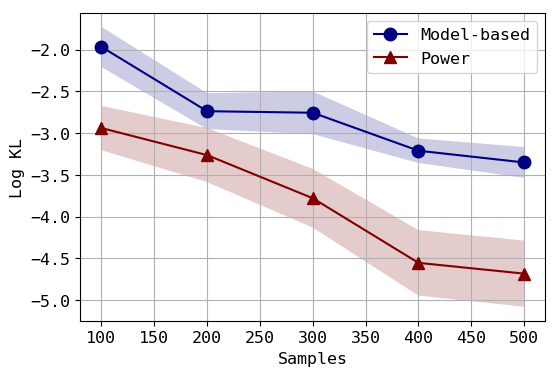
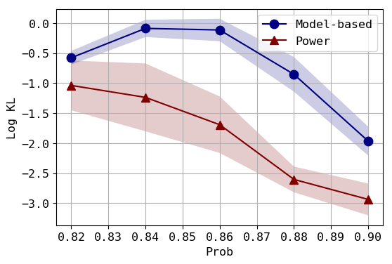
Fig. 1 provides the log KL divergence between the estimated and true stationary distributions. We compare VPM to a model-based approach, which estimates the transition matrix $\widehat{{\mathcal{T}}}(x^{\prime}|x)$ from the same set of data, then simulates a long trajectory using $\widehat{{\mathcal{T}}}$. It can be seen that our method can be more effective across different sample sizes and queue configurations.

We next apply VPM to solve a class of SDEs known as the Ornstein-Uhlenbeck process (OUP), which finds many applications in biology (Butler and King 2004), financial mathematics and physical sciences (Oksendal 2013). The process is described by the equation:

where $\mu$ is the asymptotic mean, $\sigma>0$ is the deviation, $\theta>0$ determines the strength, and $W$ is the Wiener process. The OUP has a closed-form solution, which converges to the stationary distribution, a normal distribution $\mathcal{N}(\mu,\sigma^{2}/2\theta)$, as $t\to\infty$. This allows us to conveniently calculate the Maximum Mean Discrepancy (MMD) between the adjusted sample to a true sample. We compare our method with the Euler-Maruyama (EM) method (Gardiner 2009), which is a standard simulation-based method for solving SDEs. VPM uses samples from the EM steps to train the ratio network and the learned ratio is used to compute weighted MMD.

The results are shown in Fig. 2, with different configurations of parameters $(\mu,\sigma,\theta)$. It can be seen that VPM consistently improves over the EM method in terms of the log MMD to a true sample from the normal distribution. The EM method only uses the most recent data, which can be wasteful since the past data can carry additional information about the system dynamics.

In addition, we perform experiment on real-world phylogeny studies. OUP is widely used to model the evolution of various organism traits. The results of two configurations (Beaulieu et al. 2012; Santana et al. 2012, Tab.3&1 resp.) are shown in Fig. 2(d). Notably VPM can improve over the EM method by correcting the sample with learned ratio.

In this experiment, we demonstrate how VPM can post-process MCMC to use transition data more effectively in order to learn the target distributions. We use four common potential functions as shown in the first column of Fig. 3 (Neal 2003; Rezende and Mohamed 2015; Li et al. 2018). A point is sampled from the uniform distribution $p(x)=\text{Unif}(x;[-6,6]^{2})$, then transitioned through an HMC operator (Neal et al. 2011). The transitioned pairs are used as training set $\mathcal{D}$.

We compare VPM to a model-based method that explicitly learns a transition model $\widehat{{\mathcal{T}}}(x^{\prime}|x)$, parametrized as a neural network to produce Gaussian mean (with fixed standard deviation of $0.1$). Then, we apply $\widehat{{\mathcal{T}}}$ to a hold-out set drawn from $p(x)$ sufficiently many times, and use the final instances as limiting samples (second column of Fig. 3). As for VPM, since $p$ is uniform, the estimated $\widehat{\tau}$ is proportional to the true stationary distribution. To obtain limiting samples (third column of Fig. 3), we resample from a hold-out set drawn from $p(x)$ with probability proportional to $\widehat{\tau}$.

The results are shown in Fig. 3. Note that the model-based method quickly collapses all training data into high-probability regions as stationary distributions, which is an inevitable tendency of restricted parametrized $\widehat{{\mathcal{T}}}$. Our learned ratio faithfully reconstructs the target density as shown in the right-most column of Fig. 3. The resampled data of VPM are much more accurate and diverse than that of the model-based method. These experiments show that VPM can indeed effectively use a fixed set of data to recover the stationary distribution without additional information.

To compare the results quantitatively, Fig. 4 shows the MMD of the estimated sample to a “true” sample. Since there is no easy way to sample from the potential function, the “true” sample consists of data after $2k$ HMC steps with rejection sampler. After each MCMC step, VPM takes the transition pairs as input and adjusts the sample importance according to the learned ratio. As we can see, after each MCMC step, VPM is able to post-process the data and further reduce MMD by applying the ratio. The improvement is consistent along different MCMC steps across different datasets.

Finally, we apply our method to behavior-agnostic off-policy evaluation outlined in Section 1, in which only the transition data and the target policy are given, while the behavior policy is unknown. Concretely, given a sample $\mathcal{D}=\left\{\left(s,a,r,s^{\prime}\right)_{i=1}^{n}\right\}$ from the behavior policy, we compose each transition in $\mathcal{D}$ with a target action $a^{\prime}\sim\pi\left(\cdot|s^{\prime}\right)$. Denoting $x=\left(s,a\right)$, the data set can be expressed as $\mathcal{D}=\left\{\left(x,x^{\prime}\right)_{i=1}^{n}\right\}$. Applying the proposed VPM with ${\mathcal{T}}(x^{\prime}|x)$, we can estimate $\frac{\mu\left(s,a\right)}{p\left(s,a\right)}$, hence the average accumulated reward can be obtained via (3). Additional derivation and discussion can be found in Appendix C.

We conduct experiments on the (discrete) Taxi environment as in Liu et al. 2018, and the challenging (continuous) environments including the Reacher, HalfCheetah and Ant.

Taxi is a gridworld environment in which the agent navigates to pick up and drop off passengers in specific locations. The target and behavior policies are set as in Liu et al. 2018. For the continuous environments, the Reacher agent tries to reach a specified location by swinging an robotic arm, while the HalfCheetah/Ant agents are complex robots that try to move forward as much as possible. The target policy is a pre-trained PPO or A2C neural network, which produces a Gaussian action distribution $\mathcal{N}(m_{t},\Sigma_{t})$. The behavior policy is the same as target policy but using a larger action variance $\Sigma_{b}=(1-\alpha)\Sigma_{t}+2\alpha\Sigma_{t},\alpha\in(0,1]$. We collect $T$ trajectories of $n$ steps each, using the behavior policy.

We compare VPM to a model-based method that estimates both the transition ${\mathcal{T}}$ and reward $R$ functions. Using behavior cloning, we also compare to the trajectory-wise and step-wise weighted importance sampling (WIST,WISS) (Precup et al. 2001), as well as Liu et al. 2018 with their public code for the Taxi environment.

The results are shown in Fig. 5. The $x$-axes are different configurations and the $y$-axes are the log Mean Square Error (MSE) to the true average target policy reward, estimated from abundant on-policy data collected from the target policy. As we can see, VPM outperforms all baselines significantly across different settings, including number of trajectories, trajectory length and behavior policies. The method by Liu et al. 2018 can suffer from not knowing the behavior policy, as seen in the Taxi environment. Weighted importance sampling methods (WIST,WISS) also require access to the behavior policy.

References

- Andrieu et al. [2003] Christophe Andrieu, Nando de Freitas, Arnaud Doucet, and Michael I. Jordan. An introduction to mcmc for machine learning. Machine Learning, 50:5–43, 2003.
- Atencia and Moreno [2004] Ivan Atencia and Pilar Moreno. The discrete-time geo/geo/1 queue with negative customers and disasters. Computers & Operations Research, 31(9):1537–1548, 2004.
- Bach [2014] Francis R. Bach. Breaking the curse of dimensionality with convex neural networks. CoRR, abs/1412.8690, 2014.
- Balsubramani et al. [2013] Akshay Balsubramani, Sanjoy Dasgupta, and Yoav Freund. The fast convergence of incremental pca. In Advances in Neural Information Processing Systems, pages 3174–3182, 2013.
- Beaulieu et al. [2012] Jeremy M Beaulieu, Dwueng-Chwuan Jhwueng, Carl Boettiger, and Brian C O’Meara. Modeling stabilizing selection: expanding the ornstein–uhlenbeck model of adaptive evolution. Evolution: International Journal of Organic Evolution, 66(8):2369–2383, 2012.
- Bottou and Bousquet [2008] Léon Bottou and Olivier Bousquet. The tradeoffs of large scale learning. In Advances in neural information processing systems, pages 161–168, 2008.
- Butler and King [2004] Marguerite A Butler and Aaron A King. Phylogenetic comparative analysis: a modeling approach for adaptive evolution. The American Naturalist, 164(6):683–695, 2004.
- Dai et al. [2017] Bo Dai, Niao He, Yunpeng Pan, Byron Boots, and Le Song. Learning from conditional distributions via dual embeddings. In Artificial Intelligence and Statistics, pages 1458–1467, 2017.
- Gardiner [2009] Crispin Gardiner. Stochastic methods, volume 4. Springer Berlin, 2009.
- Gelada and Bellemare [2019] Carles Gelada and Marc G Bellemare. Off-policy deep reinforcement learning by bootstrapping the covariate shift. In Proceedings of the AAAI Conference on Artificial Intelligence, volume 33, pages 3647–3655, 2019.
- Gretton et al. [2009] Arthur Gretton, Alex Smola, Jiayuan Huang, Marcel Schmittfull, Karsten Borgwardt, and Bernhard Schölkopf. Covariate shift by kernel mean matching. Dataset shift in machine learning, 3(4):5, 2009.
- Guo et al. [2017] Zhaohan Guo, Philip S Thomas, and Emma Brunskill. Using options and covariance testing for long horizon off-policy policy evaluation. In Advances in Neural Information Processing Systems, pages 2492–2501, 2017.
- Hallak and Mannor [2017] Assaf Hallak and Shie Mannor. Consistent on-line off-policy evaluation. In Proceedings of the 34th International Conference on Machine Learning-Volume 70, pages 1372–1383. JMLR. org, 2017.
- Hardt and Price [2014] Moritz Hardt and Eric Price. The noisy power method: A meta algorithm with applications. In Advances in Neural Information Processing Systems, pages 2861–2869, 2014.
- Haviv [2009] Moshe Haviv. Queues–a course in queueing theory. The Hebrew University, Jerusalem, 91905, 2009.
- Hoffman and Gelman [2014] Matthew D Hoffman and Andrew Gelman. The no-u-turn sampler: adaptively setting path lengths in hamiltonian monte carlo. Journal of Machine Learning Research, 15(1):1593–1623, 2014.
- Jiang and Li [2016] Nan Jiang and Lihong Li. Doubly robust off-policy value evaluation for reinforcement learning. In International Conference on Machine Learning, pages 652–661, 2016.
- Kadanoff [2000] Leo P Kadanoff. Statistical physics: statics, dynamics and renormalization. World Scientific Publishing Company, 2000.
- Kim et al. [2005] Kwang In Kim, Matthias O. Franz, and Bernhard Schölkopf. Iterative kernel principal component analysis for image modeling. IEEE transactions on pattern analysis and machine intelligence, 27(9):1351–1366, 2005.
- Koller and Friedman [2009] Daphne Koller and Nir Friedman. Probabilistic graphical models: principles and techniques. MIT press, 2009.
- Levin and Peres [2017] David A Levin and Yuval Peres. Markov chains and mixing times, volume 107. American Mathematical Soc., 2017.
- Li et al. [2019] Chunyuan Li, Ke Bai, Jianqiao Li, Guoyin Wang, Changyou Chen, and Lawrence Carin. Adversarial learning of a sampler based on an unnormalized distribution. In The 22nd International Conference on Artificial Intelligence and Statistics, pages 3302–3311, 2019.
- Li and Tian [2008] Ji-hong Li and Nai-shuo Tian. Analysis of the discrete time geo/geo/1 queue with single working vacation. Quality Technology & Quantitative Management, 5(1):77–89, 2008.
- Li et al. [2015] Lihong Li, Remi Munos, and Csaba Szepesvari. Toward minimax off-policy value estimation. In Artificial Intelligence and Statistics, pages 608–616, 2015.
- Li et al. [2018] Wenliang Li, Dougal Sutherland, Heiko Strathmann, and Arthur Gretton. Learning deep kernels for exponential family densities. arXiv preprint arXiv:1811.08357, 2018.
- Liu [2001] Jun S. Liu. Monte Carlo strategies in scientific computing. Springer, 2001. ISBN 0387952306.
- Liu and Lee [2017] Qiang Liu and Jason Lee. Black-box importance sampling. In Artificial Intelligence and Statistics, pages 952–961, 2017.
- Liu et al. [2016] Qiang Liu, Jason Lee, and Michael Jordan. A kernelized stein discrepancy for goodness-of-fit tests. In International conference on machine learning, pages 276–284, 2016.
- Liu et al. [2018] Qiang Liu, Lihong Li, Ziyang Tang, and Dengyong Zhou. Breaking the curse of horizon: Infinite-horizon off-policy estimation. In Advances in Neural Information Processing Systems, pages 5356–5366, 2018.
- Meyn et al. [2009] Sean Meyn, Richard L. Tweedie, and Peter W. Glynn. Markov Chains and Stochastic Stability. Cambridge Mathematical Library. Cambridge University Press, 2 edition, 2009. doi: 10.1017/CBO9780511626630.
- Mohri et al. [2012] Mehryar Mohri, Afshin Rostamizadeh, and Ameet Talwalkar. Foundations of Machine Learning. The MIT Press, 2012. ISBN 026201825X, 9780262018258.
- Nachum et al. [2019] Ofir Nachum, Yinlam Chow, Bo Dai, and Lihong Li. Dualdice: Behavior-agnostic estimation of discounted stationary distribution corrections. CoRR, abs/1906.04733, 2019. URL http://arxiv.org/abs/1906.04733.
- Neal [2003] Radford M Neal. Slice sampling. Annals of statistics, pages 705–741, 2003.
- Neal et al. [2011] Radford M Neal et al. Mcmc using hamiltonian dynamics. Handbook of markov chain monte carlo, 2(11):2, 2011.
- Nguyen et al. [2008] X.L. Nguyen, M. Wainwright, and M. Jordan. Estimating divergence functionals and the likelihood ratio by penalized convex risk minimization. In Advances in Neural Information Processing Systems 20, pages 1089–1096. MIT Press, Cambridge, MA, 2008.
- Oates et al. [2017] Chris J Oates, Mark Girolami, and Nicolas Chopin. Control functionals for monte carlo integration. Journal of the Royal Statistical Society: Series B (Statistical Methodology), 79(3):695–718, 2017.
- Oksendal [2013] Bernt Oksendal. Stochastic differential equations: an introduction with applications. Springer Science & Business Media, 2013.
- Precup et al. [2001] Doina Precup, Richard S Sutton, and Sanjoy Dasgupta. Off-policy temporal-difference learning with function approximation. In ICML, pages 417–424, 2001.
- Puterman [2014] Martin L Puterman. Markov decision processes: discrete stochastic dynamic programming. John Wiley & Sons, 2014.
- Rezende and Mohamed [2015] Danilo Jimenez Rezende and Shakir Mohamed. Variational inference with normalizing flows. arXiv preprint arXiv:1505.05770, 2015.
- Robert and Casella [2004] C. Robert and G. Casella. Monte Carlo Statistical Methods. Springer, second edition, 2004.
- Rubinstein and Kroese [2016] Reuven Y Rubinstein and Dirk P Kroese. Simulation and the Monte Carlo method, volume 10. John Wiley & Sons, 2016.
- Ryu and Boyd [2016] Ernest K Ryu and Stephen Boyd. Primer on monotone operator methods. Appl. Comput. Math, 15(1):3–43, 2016.
- Santana et al. [2012] Sharlene E Santana, Ian R Grosse, and Elizabeth R Dumont. Dietary hardness, loading behavior, and the evolution of skull form in bats. Evolution: International Journal of Organic Evolution, 66(8):2587–2598, 2012.
- Serfozo [2009] Richard Serfozo. Basics of applied stochastic processes. Springer Science & Business Media, 2009.
- Shimodaira [2000] H. Shimodaira. Improving predictive inference under convariance shift by weighting the log-likelihood function. Journal of Statistical Planning and Inference, 90, 2000.
- Song et al. [2017] Jiaming Song, Shengjia Zhao, and Stefano Ermon. A-nice-mc: Adversarial training for mcmc. In Advances in Neural Information Processing Systems, pages 5140–5150, 2017.
- Sugiyama and Kawanabe [2012] Masashi Sugiyama and Motoaki Kawanabe. Machine learning in non-stationary environments: Introduction to covariate shift adaptation. MIT press, 2012.
- Sugiyama et al. [2008] Masashi Sugiyama, Taiji Suzuki, Shinichi Nakajima, Hisashi Kashima, Paul von Bünau, and Motoaki Kawanabe. Direct importance estimation for covariate shift adaptation. Annals of the Institute of Statistical Mathematics, 60(4):699–746, 2008.
- Sugiyama et al. [2012] Masashi Sugiyama, Taiji Suzuki, and Takafumi Kanamori. Density ratio estimation in machine learning. Cambridge University Press, 2012.
- Sutton and Barto [1998] R.S. Sutton and A.G. Barto. Reinforcement Learning: An Introduction. MIT Press, 1998.
- Thomas and Brunskill [2016] Philip Thomas and Emma Brunskill. Data-efficient off-policy policy evaluation for reinforcement learning. In International Conference on Machine Learning, pages 2139–2148, 2016.
- Wang et al. [2014] Fang Wang, Jinting Wang, and Feng Zhang. Equilibrium customer strategies in the geo/geo/1 queue with single working vacation. Discrete Dynamics in Nature and Society, 2014, 2014.
- Wang et al. [2017] Yu-Xiang Wang, Alekh Agarwal, and Miroslav Dudik. Optimal and adaptive off-policy evaluation in contextual bandits. In Proceedings of the 34th International Conference on Machine Learning-Volume 70, pages 3589–3597. JMLR.org, 2017.
- Welling and Teh [2011] Max Welling and Yee-Whye Teh. Bayesian learning via stochastic gradient langevin dynamics. In International Conference on Machine Learning (ICML), pages 681–688, 2011.
- Xie et al. [2015] Bo Xie, Yingyu Liang, and Le Song. Scale up nonlinear component analysis with doubly stochastic gradients. arXiv preprint arXiv:1504.03655, 2015.
- Xie et al. [2019] Tengyang Xie, Yifei Ma, and Yu-Xiang Wang. Towards optimal off-policy evaluation for reinforcement learning with marginalized importance sampling. In Advances in Neural Information Processing Systems 32, pages 9665–9675, 2019.
- Yang et al. [2017] Lin F Yang, Vladimir Braverman, Tuo Zhao, and Mengdi Wang. Online factorization and partition of complex networks from random walks. arXiv preprint arXiv:1705.07881, 2017.
Appendix
Appendix A Consistency of the Objectives
Theorem 1 (Consistency of solution)
Proof Taking derivative of the objective function in (12) and setting it to zero, we can see that the unconstrained solution is . Moreover, it satisfies the constraint when : we can rewrite for some distribution and .
Appendix B Convergence Analysis
Let be a measure space. The space consists of measurable functions such that . Suppose the initial , we want to show the converging behavior of the following damped iteration: