Formal Controller Synthesis for Continuous-Space MDPs via Model-Free Reinforcement Learning

The evolution of the state of dt-SCS $\Sigma$ for an initial state $x(0)\in X$ and an input sequence $\{\nu(k):\Omega\rightarrow U,\,\,k\in\mathbb{N}\}$ is described as:

We define Markov policies to control the system in (2.1).

We associate to $U$ the set $\mathcal{U}$ to be the collection of sequences $\{\nu(k):\Omega\rightarrow U,\,\,k\in\mathbb{N}\}$, in which $\nu(k)$ is independent of $\varsigma(t)$ for any $k,t\in\mathbb{N}$ and $t\geq k$. The random sequence $x_{a\nu}:\Omega\times\mathbb{N}\rightarrow X$ satisfying (2.2) for any initial state $a\in X$, and $\nu(\cdot)\in\mathcal{U}$ is called the solution process of $\Sigma$ under the input $\nu$ and the initial state $a$.

Formal requirements provide the rigorous and unambiguous formalism to express requirements over MDPs [BK08]. A common way to describe formal requirements is by using automata-based specifications or logic-based specifications using formulae in, for instance, linear temporal logic (LTL). For example, consider a dt-SCS $\Sigma$ in (2.1) and a measurable target set $\mathsf{B}\subset X$. We say that a state trajectory $\{x(k)\}_{k\geq 0}$ reaches a target set $\mathsf{B}$ within time interval $[0,T]\subset\mathbb{N}$, if there exists a $k\in[0,T]$ such that $x(k)\in\mathsf{B}$. This bounded reaching of $\mathsf{B}$ is denoted by $\lozenge^{\leq T}\{x\in\mathsf{B}\}$ or briefly $\lozenge^{\leq T}\mathsf{B}$. For $T\rightarrow\infty$, we denote the reachability property as $\lozenge\mathsf{B}$, i.e., eventually $\mathsf{B}$. For a dt-SCS $\Sigma$ with a policy $\rho$, we want to compute the probability that a state trajectory reaches $\mathsf{B}$ within the time horizon $T\in{\mathbb{N}}$, i.e., $\mathbb{P}(\lozenge^{\leq T}\mathsf{B})$. The reachability probability is the probability that the target set $\mathsf{B}$ is eventually reached and is denoted by $\mathbb{P}(\lozenge\mathsf{B})$. In this paper, we deal with properties more complex than simple reachability property.

Finite Automata. A deterministic finite automaton (DFA) is a tuple $\mathcal{A}=(Q,\mathsf{\Sigma}_{\textsf{a}},\mathsf{t},q_{0},F_{\textsf{a}})$ where $Q$ is a finite set of states, $\mathsf{\Sigma}_{\textsf{a}}$ is an alphabet, $\mathsf{t}:Q\times\mathsf{\Sigma}_{\textsf{a}}\to Q$ is a transition function, $q_{0}\in Q$ is the initial state, and $F_{\textsf{a}}\subseteq Q$ are accepting states. We write $\lambda$ for the empty string and $\mathsf{\Sigma}_{\textsf{a}}^{*}$ for the set of all strings over $\mathsf{\Sigma}_{\textsf{a}}$. The extended transition function $\mathsf{\hat{t}}:Q\times\mathsf{\Sigma}_{\textsf{a}}^{*}\to Q$ (transition function extended to summarize the effect of reading a string) can be defined as:

The language $\mathcal{L}(\mathcal{A})$ accepted by a DFA $\mathcal{A}$ is defined as $\mathcal{L}(\mathcal{A})=\{\bar{w}\>:\>\mathsf{\hat{t}}(q_{0},\bar{w})\in F_{\textsf{a}}\}$. DFAs are well-established models to express regular specifications over finite words. DFAs can also be interpreted over $\omega$-words: an $\omega$-word is accepted if there is a prefix that is accepted by the DFA. Among others, DFAs are expressive enough to capture syntactically a co-safe fragment of linear temporal logic (LTL) defined next.

Linear Temporal Logic. Consider a set of atomic propositions $AP$ and the alphabet $\mathsf{\Sigma}_{\textsf{a}}:=2^{AP}$. Let $\omega=\omega(0),\omega(1),\omega(2),\ldots\in\mathsf{\Sigma}_{\textsf{a}}^{\mathbb{N}}$ be an infinite word, that is, a string composed of letters from $\mathsf{\Sigma}_{\textsf{a}}$. We are interested in those atomic propositions that are relevant to the dt-SCS via a measurable labeling function $\mathsf{L}$ from the state space to the alphabet as $\mathsf{L}:X\rightarrow\mathsf{\Sigma}_{\textsf{a}}$. State trajectories $\{x(k)\}_{k\geq 0}\in X^{\mathbb{N}}$ can be readily mapped to the set of infinite words $\mathsf{\Sigma}_{\textsf{a}}^{\mathbb{N}}$, as $\omega=\mathsf{L}(\{x(k)\}_{k\geq 0}):=\{\omega\in\mathsf{\Sigma}_{\textsf{a}}^{\mathbb{N}}\,|\,\omega(k)=\mathsf{L}(x(k))\}$. Consider LTL properties with the syntax [BK08]

Let $\omega_{k}=\omega(k),\omega(k+1),\omega(k+2),\ldots$ be a subsequence (suffix) of $\omega$, then the satisfaction relation between $\omega$ and a property $\phi$, expressed in LTL, is denoted by $\omega\vDash\phi$ (or equivalently $\omega_{0}\vDash\phi$). Semantics of the satisfaction relation are defined recursively over $\omega_{k}$ and the syntax of the LTL formula $\phi$. An atomic proposition $p\in AP$ is satisfied by $\omega_{k}$, i.e., $\omega_{k}\vDash p$, iff $p\in\omega(k)$. Furthermore, $\omega_{k}\vDash\neg\phi$ if $\omega_{k}\nvDash\phi$ and we say that $\omega_{k}\vDash\phi_{1}\wedge\phi_{2}$ if $\omega_{k}\vDash\phi_{1}$ and $\omega_{k}\vDash\phi_{2}$. The next operator $\omega_{k}\vDash\mathord{\bigcirc}\phi$ holds if the property holds at the next time instance $\omega_{k+1}\vDash\phi$. We denote by $\mathord{\bigcirc}^{j}$, $j\in{\mathbb{N}}$, $j$ times composition of the next operator. With a slight abuse of the notation, one has $\mathord{\bigcirc}^{0}\phi=\phi$ for any property $\phi$. The temporal until operator $\omega_{k}\vDash\phi_{1}\mathbin{\sf U}\phi_{2}$ holds if $\exists i\in\mathbb{N}:$ $\omega_{k+i}\vDash\phi_{2},\mbox{and }\forall j\in{\mathbb{N}:}0\leq j<i,\omega_{k+j}\vDash\phi_{1}$. Based on these semantics, disjunction ($\vee$) can be defined by $\omega_{k}\vDash\phi_{1}\vee\phi_{2}\ \Leftrightarrow\ \omega_{k}\vDash\neg(\neg\phi_{1}\wedge\neg\phi_{2})$. This paper focuses on a fragment of LTL properties known as syntactically co-safe linear temporal logic (scLTL) [KV01] defined below.

Even though scLTL formulas are defined over infinite words (as in LTL formulae), their satisfaction is guaranteed in the finite time [KV01]. Any infinite word $\omega\in\mathsf{\Sigma}_{\textsf{a}}^{\mathbb{N}}$ satisfying an scLTL formula $\phi$ has a finite word $\omega_{f}\in\mathsf{\Sigma}_{\textsf{a}}^{n}$, $n\in\mathbb{N}$, as its prefix such that all infinite words with a prefix $\omega_{f}$ also satisfy the formula $\phi$. We denote the set of all such finite prefixes associated with an scLTL formula $\phi$ by $\mathcal{L}_{f}(\phi)$.

For verification and synthesis purposes, the scLTL properties can be compiled into a DFA $\mathcal{A}_{\phi}$ over the alphabet $2^{AP}$ such that $\mathcal{L}_{f}(\phi)=\mathcal{L}(\mathcal{A}_{\phi})$ [KV01]. This construction is routine; we refer the interested reader to [KV01] for details of the construction of the DFA $\mathcal{A}_{\phi}$ from $\phi$ such that $\mathcal{L}(\mathcal{A}_{\phi})=\mathcal{L}_{f}(\phi)$. The resulting DFA has the property that there is a unique accepting state and all out-going transitions from that state are self-loops. Such a DFA is also known as a co-safety automaton. In the rest of the paper we assume that the DFA $\mathcal{A}_{\phi}$ for an scLTL property $\phi$ is a co-safety automaton.

Given a policy $\rho$, the probability that a state trajectory of $\Sigma$ satisfies an scLTL property $\phi$ over the time horizon $[0,T]$, is denoted by $\mathbb{P}(\omega_{f}\in\mathcal{L}(\mathcal{A}_{\phi})~\text{s.t.}~|\omega_{f}|\leq T+1)$, where $|\omega_{f}|$ is the length of $\omega_{f}$ [DLT08b]. The co-safety automaton for the bounded time-horizon satisfaction can be computed by unrolling the DFA for $\phi$. In the rest of the paper we assume such a representation for the finite horizon satisfaction.

A dt-SCS $\Sigma$ in (2.1) can be equivalently represented as a Markov decision process (MDP) [Kal97, Proposition 7.6]

where the map $T_{\mathsf{x}}:\mathcal{B}(X)\times X\times U\rightarrow[0,1]$, is a conditional stochastic kernel that assigns to any $x\in X$, and $\nu\in U$, a probability measure $T_{\mathsf{x}}(\cdot|x,\nu)$ on the measurable space $(X,\mathcal{B}(X))$ so that for any set $\mathcal{A}\in\mathcal{B}(X)$,

For given input $\nu(\cdot),$ the stochastic kernel $T_{\mathsf{x}}$ captures the evolution of the state of $\Sigma$ and can be uniquely determined by the pair $(\varsigma,f)$ from (2.1). In other words, $T_{\mathsf{x}}$ contains the information of the function $f$ and the distribution of the noise $\varsigma(\cdot)$ in the dynamical representation.

Now we approximate a dt-SCS $\Sigma$ with a finite $\widehat{\Sigma}$ using an abstraction algorithm. The algorithm first constructs a finite partition of the state space $X=\cup_{i}\mathsf{X}_{i}$. Then representative points $\bar{x}_{i}\in\mathsf{X}_{i}$ are selected as abstract states. Given a dt-SCS $\Sigma=\left(X,U,\varsigma,f\right)$, the constructed finite MDP $\widehat{\Sigma}$ is

where $\hat{X}=\{\bar{x}_{i},i=1,\ldots,n_{x}\}$, a finite subset of $X$, and $\hat{U}:=U$ are finite state and input sets of the MDP $\widehat{\Sigma}$. Moreover, $\hat{f}:\hat{X}\times\hat{U}\times V_{\varsigma}\rightarrow\hat{X}$ is defined as $\hat{f}(\hat{x},\hat{\nu},\varsigma)=\Pi_{x}(f(\hat{x},\hat{\nu},\varsigma))$, where $\Pi_{x}:X\rightarrow\hat{X}$ is the map that assigns to any $x\in X$, the representative point $\bar{x}\in\hat{X}$ of the corresponding partition set containing $x$. The initial state of $\widehat{\Sigma}$ is also selected according to $\hat{x}_{0}:=\Pi_{x}(x_{0})$ with $x_{0}$ being the initial state of $\Sigma$.

The proposed dynamical representation employs the map $\Pi_{x}:X\rightarrow\hat{X}$ that assigns to any $x\in X$, the representative point $\bar{x}\in\hat{X}$ of the corresponding partition set containing $x$ satisfying the inequality:

where $\delta:=\sup\{\|x-x^{\prime}\|,\,\,x,x^{\prime}\in\mathsf{X}_{i},\,i=1,2,\ldots,n_{x}\}$ is the state discretization parameter.

Note that one can write the equivalent finite-MDP representation of $\widehat{\Sigma}$ in (3.2) as [Put14, Chapter 3.5]

where

and $\Xi:X\rightarrow 2^{X}$ is a map that assigns to any $x\in X$, the corresponding partition set it belongs to, i.e., $\Xi(x)=\mathsf{X}_{i}$ if $x\in\mathsf{X}_{i}$ for some $i=1,2,\ldots,n_{x}$. We employ this finite-MDP representation of (3.4) in Section 4.

The following theorem [SA13] shows the closeness between a continuous-space MDP $\Sigma$ and its finite abstraction $\widehat{\Sigma}$ in a probabilistic setting.

The error bound $\varepsilon$ in (3.5) is obtained by characterizing $\mathbb{P}(\Sigma_{\hat{\nu}}\vDash\phi)$ recursively similar to dynamic programs (DP). This error is related to the approximation of the continuous kernel with a discrete one, hence the term $\delta\mathscr{H}$. There is also an integration over the specification set, thus $\mathscr{L}$ appears in $\varepsilon$. Finally, the errors contributed in every iteration of the DP are added, hence the horizon $T$.

It follows from Theorem 3.3 that one can construct a finite MDP $\widehat{\Sigma}$ from a continuous-space dt-SCS $\Sigma$ with known conditional stochastic kernels such that the optimal probability of satisfaction of an scLTL specification $\phi$ for $T$ steps in $\widehat{\Sigma}$ is no more than $2\varepsilon$-worse than the optimal policy in $\Sigma$; see the definition of $\varepsilon$ in Theorem 3.3. Hence, given a dt-SCS $\Sigma$ with known conditional stochastic kernels, an scLTL property $\phi$, and a time-horizon $T$, a $2\varepsilon$-optimal policy to satisfy $\phi$ in $T$ steps is computed using a suitable finite MDP with the corresponding $\delta$ as the state discretization parameter. This problem can be solved using the finite-horizon dynamic programming over the product of $\widehat{\Sigma}$ and the DFA $\mathcal{A}_{\phi}$ (cf. Definition 2.4 and the paragraph afterward) by giving a scalar reward to all transitions once a final state of $\mathcal{A}_{\phi}$ is reached.

Recall that the DFA $A_{\phi}$ corresponding to an scLTL specification $\phi$ has the property that there is a unique accepting state and all out-going transitions from that state are self-loops. It follows that total optimal expected reward in the product is equal to the optimal probability of satisfying the specification.

When stochastic kernels are unknown, Theorem 3.3 still provides the correct probabilistic bound given a discretization parameter $\delta$ if the Lipschitz constant $\mathscr{H}$ is known. This observation enables us to employ reinforcement learning algorithms over the underlying discrete MDP without explicitly constructing the abstraction by simply restricting observations of the reinforcement learner to the closest representative point in the set of partitions (cf. Subsection 3.1). We call such an underlying finite MDP a $\widehat{\Sigma}_{\delta}$ abstraction.

Model-free reinforcement learning can be employed under such observations by using the DFA $\mathcal{A}_{\phi}$ to provide scalar rewards as defined in Definition 4.1. The observations of the MDP are used by an interpreter process to compute a run of the DFA. When the DFA reaches a final state, the interpreter gives the reinforcement learner a positive reward and the training episode terminates. Since the product MDP $\mathcal{M}_{\star}$ is a finite MDP, from Proposition 4.2, it follows that any correct and convergent RL algorithm that maximizes this expected reward is guaranteed to converge to a policy that maximizes the probability of satisfaction of the scLTL objective. From Theorem 3.3 it then follows that any converging reinforcement learning algorithm [JJS94, BM00] over such finite observation set then converges to a $2\varepsilon$-optimal policy over the concrete dt-SCS $\Sigma$ thanks to Theorem 3.3. We summarize the proposed solution in the following theorem.

Consider a finite MDP $\widehat{\Sigma}=(\hat{X},\hat{U},\hat{T})$, a co-safety automaton $\mathcal{A}_{\phi}=(Q,\mathsf{\Sigma}_{\textsf{a}},\mathsf{t},q_{0},q_{F})$, and their product MDP $\mathcal{M}_{\star}=(X_{\star},U_{\star},T_{\star},x_{\star},\rho_{\star})$. Since the reward function $\rho_{\star}$ is sparse, it may not be effective in the reinforcement learning. For this reason, we introduce a “shaped” reward function $\rho_{\kappa}$ (parameterized by a hyper-parameter $\kappa$) such that for suitable values of $\kappa$, optimal policies for $\rho_{\kappa}$ are the same as optimal policies for $\rho_{\star}$, but unlike $\rho_{\star}$ the function $\rho_{\kappa}$ is dense.

The function $\rho_{\kappa}$ is defined based on the structure of co-safety automaton $\mathcal{A}_{\phi}$. Let $d(q)$ be the minimum distance of the state $q$ to the unique accepting state $q_{F}$. Let $d_{\texttt{max}}=1+\max_{q}\{d(q)\>:\>d(q)<\infty\}$. If there is no path from $q$ to $q_{F}$, let $d(q)$ be equal to $d_{\texttt{max}}$. We define the potential function $P:\mathbb{N}\to\mathbb{R}$ as the following:

where $\kappa$ is a constant hyper-parameter. Note that the potential of the initial state $P(d(q_{0}))=0$ and the potential of the final state $P(d(q_{F}))=1$. Moreover, note that

We define the “shaped” reward function $\rho_{\kappa}:\hat{X}\times\hat{U}\times\hat{X}\to\mathbb{R}$ as the difference between potentials of the destination and of the target states of transition of the automaton, i.e.,

Moreover, notice that for every run $r=(x_{0},q_{0}),\nu_{1},(x_{1},q_{1}),$ $\nu_{2},\ldots,\nu_{n},(x_{n},q_{n})$ of $\mathcal{M}_{\star}$, its accumulated reward is simply the potential difference between the last and the first states, i.e., $P(d(q_{n}))-P(d(q_{0}))$.

The proof of Theorem 4.4 is provided in Appendix.

Theorem 4.4 demonstrates one way to shape rewards such that the optimal policy remains unaffected while making the rewards less sparse. Along similar lines, one can construct a variety of potential functions and corresponding shaped rewards with similar correctness properties. Of course, the reward shaping schema presented here is no silver bullet: we expect the performance of different potential functions to be incomparable along a carefully chosen ensemble of MDPs. Since rewards are shaped without any knowledge of the underlying MDP, there may be MDPs where un-shaped rewards may work as well or even better than a given shaped reward. We envisage that the ability to combine several competing ways to shape reward may work better in practice. While sparse rewards may be sufficient for simpler learning tasks, we demonstrate that shaped rewards such as the one provided here are crucial for larger case studies such as the BMW case-study reported in the next section.

Here, we apply our results to the temperature regulation of a room equipped with a heater. The model of this case study is adapted from [MGW18] by including stochasticity in the model as an additive noise. The evolution of the temperature can be described by the following dt-SCS:

where $\eta=0$, $\beta=0.022$, and $\gamma=0.05$ are conduction factors respectively between this room and the other rooms in a network, between the external environment and the room, and between the heater and the room. Moreover, $x(k)$ and $\nu(k)$ are taking values in $[19,21]$ and a finite input set $\{0.03,0.09,0.15,0.21,0.27,0.33,0.39,\\ 0.45,0.51,0.57\},$ respectively. The parameter $T_{e}=-1\,^{\circ}C$ is the outside temperature, and $T_{h}=50\,^{\circ}C$ is the heater temperature.

The main goal is to synthesize a controller for $\Sigma$ using our main results in Theorem 4.3 such that the controller maintains the temperature of the room in the safe set $[19,21]$.

We also apply our results to a road traffic control containing a cell with $2$ entries and $1$ way out, as schematically depicted in Figure 2. The model of this case study is taken from [LCGG13]; stochasticity is included in the model as the additive noise.

One of the entries of the cell is controlled by a traffic light, denoted by $\nu=\{0,1\}$, that enables (green light) or not (red light) the vehicles to pass. In this model, the length of a cell is $0.5$ kilometers ([km]), and the flow speed of the vehicles is $100$ kilometers per hour ([km/h]). Moreover, during the time interval $\tau=6.48$ seconds, it is assumed that $6$ vehicles pass the entry controlled by the traffic light, $3$ vehicles go into the entry of the cell, and one quarter of vehicles goes out on the exit of the cell (the ratio denoted by $q$). We want to observe the density of traffic $x$. The model of the system $\Sigma$ is described by:

where $l$ and $v$ are the length of the cell and the flow speed of vehicles, respectively. We synthesize a controller for $\Sigma$ using our main results in Theorem 4.3 such that the density of the traffic is lower than $20$ vehicles.

Table 1 shows a comparison of Q-learning to the computed optimal probabilities for the room temperature and road traffic examples. For each model, five different discretization steps ($\delta$) are considered and for each value of $\delta$ probabilities of satisfaction of the safety objectives are reported in the columns labeled $p_{r}$. These probabilities are $Q$-values of the initial state of the finite-state MDP for the policy computed by $Q$-learning after $10^{6}$ episodes. The objective is to keep the system safe for at least $10$ steps. For the comparison, the optimal probability $p_{*}$ for a time-dependent policy is reported assuming that we know the exact dynamics for these two examples. Note that we compute $p_{*}$ using the dynamic programming over constructed finite MDPs as proposed in Subsection 3.1. The optimal probability $p_{*}$ reported in Table 1 corresponds to the same initial condition that is utilized in the learning process. The optimal probability for the original continuous-space MDP is always within an interval $[p_{l},p_{h}]$ centered at $p_{*}$ and with a radius $\varepsilon$ as reported in Table 1. One can readily see from Table 1 that as the discretization parameter $\delta$ decreases, the size of this interval shrinks, which implies that the optimal probability for the original continuous-space MDP converges to $p_{*}$. While finer abstractions give better theoretical guarantees, for a fixed number of episodes it is easier to learn good strategies for coarser abstractions. This is reflected in Table 1, where the values of $p_{r}$ do not necessarily get better with smaller values of $\delta$. However, by increasing the number of episodes, strategies converge toward the optimal one, as illustrated in Figure 3, which visualizes room temperature control strategies computed by $Q$-learning after different numbers of episodes. Note that in Table 1, the error bound $\varepsilon$ exceeds one for $\delta\geq 0.05$ in the room temperate control example, which is not a useful probability bound for the continuous-space MDP. However, we prefer to report the corresponding values of $p_{r}$ and $p_{*}$ so that they can still be compared.

The previous case-studies are representative of what can be solved by discretization and tabular methods like Q-learning. Relaxing those constraints, we were able to apply deep deterministic policy gradient (DDPG) [LHP+15] to a $7$-dimensional nonlinear model of a BMW $320$i car [Alt19] to synthesize a reach-while-avoid controller. Though convergence guarantees are not available for DDPG and most RL algorithms with nonlinear function approximations, breakthroughs in this direction (e.g., SBEED in [DSL+17]) will expand the applicability of our results to more complex safety-critical applications.

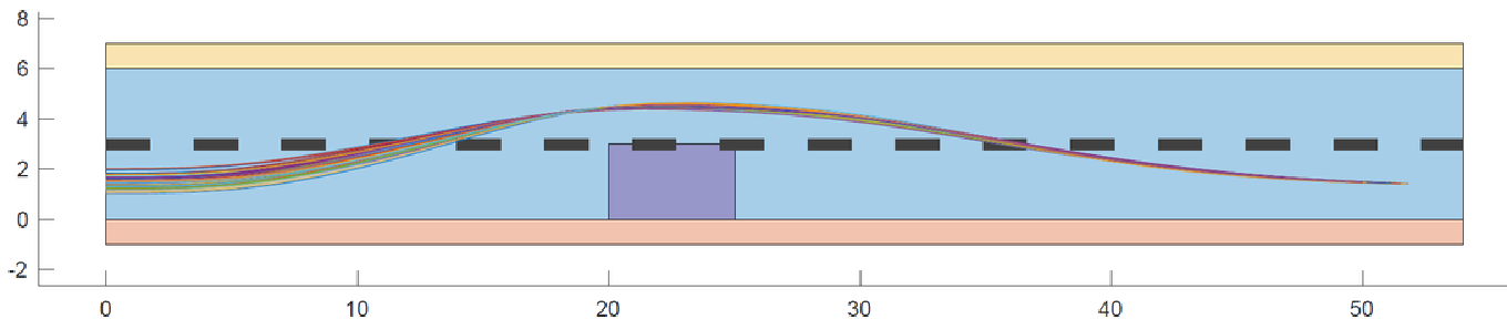
The model of this case study is borrowed from [Alt19, Section 5.1] by discretizing the dynamics in time and including a stochasticity inside the dynamics as additive noises. The dynamics of the vehicle are given in Appendix. We are interested in an autonomous operation of the vehicle on a highway. Consider a situation on a two-lane highway when an accident suddenly happens on the same lane on which our vehicle is traveling. The vehicle’s controller should find a safe maneuver to avoid the crash with the next-appearing obstacle.

Figure 4 shows the simulation from $100$ samples with varying initial positions and initial heading velocities ($16$–$18$ m/s) for the learned controller. We employed potential-based reward shaping to speed-up learning in this case study from 10K episodes (no success) to under 5K episodes (for a convincing learning, see Figure 4).

References

- [AKNP14] A. Abate, M. Kwiatkowska, G. Norman, and D. Parker. Probabilistic model checking of labelled Markov processes via finite approximate bisimulations. In Horizons of the Mind. A Tribute to Prakash Panangaden, pages 40–58. 2014.
- [Alt19] M. Althof. Commonroad: Vehicle models (version 2018a). Tech. rep. https://commonroad.in.tum.de, Technical University of Munich, 85748 Garching, Germany (October 2018), 2019.
- [APLS08] A. Abate, M. Prandini, J. Lygeros, and S. Sastry. Probabilistic reachability and safety for controlled discrete time stochastic hybrid systems. Automatica, 44(11):2724–2734, 2008.
- [BK08] C. Baier and J.-P. Katoen. Principles of Model Checking. MIT Press, 2008.
- [BM00] V. S. Borkar and S. P. Meyn. The ODE method for convergence of stochastic approximation and reinforcement learning. SIAM J. on Control and Optimization, 38(2):447–469, 2000.
- [BS96] D. P. Bertsekas and S. E. Shreve. Stochastic Optimal Control: The Discrete-Time Case. Athena Scientific, 1996.
- [CY95] C. Courcoubetis and M. Yannakakis. The complexity of probabilistic verification. J. ACM, 42(4):857–907, 1995.
- [DLT08a] J. Desharnais, F. Laviolette, and M. Tracol. Approximate analysis of probabilistic processes: Logic, simulation and games. In Proceedings of the 5th International Conference on Quantitative Evaluation of System, pages 264–273, 2008.
- [DLT08b] J. Desharnais, F. Laviolette, and M. Tracol. Approximate analysis of probabilistic processes: logic, simulation and games. In Proceedings of the International Conference on Quantitative Evaluation of SysTems (QEST 08), pages 264–273, 2008.
- [DSL+17] B. Dai, A. Shaw, L. Li, L. Xiao, N. He, Z. Liu, J. Chen, and L. Song. SBEED: Convergent reinforcement learning with nonlinear function approximation. arXiv:1712.10285, 2017.
- [HAK19] M. Hasanbeig, A. Abate, and D. Kroening. Certified reinforcement learning with logic guidance. arXiv:1902.00778, 2019.
- [HGI12] M. P. Holmes, A. G. Gray, and C. L. Isbell. Fast nonparametric conditional density estimation. arXiv: 1206.5278, 2012.
- [HKA+19] M. Hasanbeig, Y. Kantaros, A. Abate, D.l Kroening, G. J. Pappas, and I. Lee. Reinforcement learning for temporal logic control synthesis with probabilistic satisfaction guarantees. arXiv:1909.05304, 2019.
- [HS20] S. Haesaert and S. Soudjani. Robust dynamic programming for temporal logic control of stochastic systems. TAC, arXiv/1811.11445, 2020.
- [HSA17] S. Haesaert, S. Soudjani, and A. Abate. Verification of general Markov decision processes by approximate similarity relations and policy refinement. SIAM J. on Control and Optimization, 55(4):2333–2367, 2017.
- [JJS94] T. Jaakkola, M.I. Jordan, and S. P. Singh. Convergence of stochastic iterative dynamic programming algorithms. In Advances in neural information processing systems, pages 703–710, 1994.
- [JP09] A. A. Julius and G. J. Pappas. Approximations of stochastic hybrid systems. IEEE Trans. on Automatic Control, 54(6):1193–1203, 2009.
- [JSZ19] P. Jagtap, S. Soudjani, and M. Zamani. Formal synthesis of stochastic systems via control barrier certificates. arXiv: 1905.04585, 2019.
- [Kal97] O. Kallenberg. Foundations of modern probability. Springer-Verlag, New York, 1997.
- [KV01] O. Kupferman and M. Y. Vardi. Model checking of safety properties. Formal Methods in System Design, 19(3):291–314, 2001.
- [LCGG13] E. Le Corronc, A. Girard, and G. Goessler. Mode sequences as symbolic states in abstractions of incrementally stable switched systems. In Conference on Decision and Control, pages 3225–3230, 2013.
- [LFDA16] S. Levine, C. Finn, T. Darrell, and P. Abbeel. End-to-end training of deep visuomotor policies. J. Mach. Learn. Res., 17(1):1334–1373, January 2016.
- [LHP+15] T. P. Lillicrap, J. J. Hunt, A. Pritzel, N. Heess, T. Erez, Y. Tassa, D. Silver, and D. Wierstra. Continuous control with deep reinforcement learning. CoRR, abs/1509.02971, 2015.
- [LS91] K. G. Larsen and A. Skou. Bisimulation through probabilistic testing. Information and Computation, 94(1):1–28, 1991.
- [LSZ18] A. Lavaei, S. Soudjani, and M. Zamani. From dissipativity theory to compositional construction of finite Markov decision processes. In Proceedings of the 21st ACM International Conference on Hybrid Systems: Computation and Control, pages 21–30, 2018.
- [LSZ19] A. Lavaei, S. Soudjani, and M. Zamani. Compositional construction of infinite abstractions for networks of stochastic control systems. Automatica, 107:125–137, 2019.
- [LSZ20a] A. Lavaei, S. Soudjani, and M. Zamani. Compositional abstraction-based synthesis for networks of stochastic switched systems. Automatica, 114, 2020.
- [LSZ20b] A. Lavaei, S. Soudjani, and M. Zamani. Compositional abstraction of large-scale stochastic systems: A relaxed dissipativity approach. Nonlinear Analysis: Hybrid Systems, 36, 2020.
- [LSZ20c] A. Lavaei, S. Soudjani, and M. Zamani. Compositional (in)finite abstractions for large-scale interconnected stochastic systems. IEEE Transactions on Automatic Control, DOI: 10.1109/TAC.2020.2975812, 2020.
- [M+15] V. Mnih et al. Human-level control through reinforcement learning. Nature, 518:529–533, 2015.
- [MGW18] P. J. Meyer, A. Girard, and E. Witrant. Compositional abstraction and safety synthesis using overlapping symbolic models. IEEE Trans. on Automatic Control, 63(6):1835–1841, 2018.
- [MMS20] R. Majumdar, K. Mallik, and S. Soudjani. Symbolic controller synthesis for Büchi specifications on stochastic systems. Hybrid Systems: Computation and Control, arXiv:1910.12137, 2020.
- [Mun96] R. Munos. A convergent reinforcement learning algorithm in the continuous case: the finite-element reinforcement learning. In International Conference on Machine Learning, January 1996.
- [NHR99] A. Y. Ng, D. Harada, and S. J. Russell. Policy invariance under reward transformations: Theory and application to reward shaping. In International Conference on Machine Learning, pages 278–287, 1999.
- [PJP07] S. Prajna, A. Jadbabaie, and G. J. Pappas. A framework for worst-case and stochastic safety verification using barrier certificates. IEEE Trans. on Automatic Control, 52(8):1415–1428, 2007.
- [Pnu77] A. Pnueli. The temporal logic of programs. In Symposium on Foundations of Computer Science, pages 46–57, 1977.
- [PT87] C. H. Papadimitriou and J. N. Tsitsiklis. The complexity of Markov decision processes. Mathematics of operations research, 12(3):441–450, 1987.
- [Put94] M. L. Puterman. Markov Decision Processes: Discrete Stochastic Dynamic Programming. John Wiley & Sons, New York, 1994.
- [Put14] M. L. Puterman. Markov decision processes: discrete stochastic dynamic programming. John Wiley & Sons, 2014.
- [Rie05] M. Riedmiller. Neural fitted Q iteration – First experiences with a data efficient neural reinforcement learning method. In Machine Learning: ECML 2005, pages 317–328, 2005.
- [S+14] D. Silver et al. Deterministic policy gradient algorithms. In Proceedings of the 31st International Conference on International Conference on Machine Learning, pages 387–395, 2014.
- [S+16] D. Silver et al. Mastering the game of Go with deep neural networks and tree search. Nature, 529:484–489, 2016.
- [SA13] S. Soudjani and A. Abate. Adaptive and sequential gridding procedures for the abstraction and verification of stochastic processes. SIAM J. on Applied Dynamical Systems, 12(2):921–956, 2013.
- [SB18] R. S. Sutton and A. G. Barto. Reinforcement Learnging: An Introduction. MIT Press, second edition, 2018.
- [Sco92] D. W. Scott. Multivariate Density Estimation. Theory, Practice, and Visualization. Wiley, 1992.
- [SL95] R. Segala and N. Lynch. Probabilistic simulations for probabilistic processes. Nordic J. of Computing, 2(2):250–273, 1995.
- [SLW+06] A. L. Strehl, L. Li, E. Wiewiora, J. Langford, and M. L. Littman. PAC model-free reinforcement learning. In International Conference on Machine Learning, pages 881–888, 2006.
- [Sut88] R. S. Sutton. Learning to predict by the methods of temporal differences. Machine Learning, 3(1):9–44, 1988.
- [TA11] I. Tkachev and A. Abate. On infinite-horizon probabilistic properties and stochastic bisimulation functions. In Proceedings of the 50th IEEE Conference on Decision and Control, pages 526–531, 2011.
- [Tes95] G. Tesauro. Temporal difference learning and TD-Gammon. Commun. ACM, 38(3):58–68, 1995.
- [Wat89] C. J. C. H. Watkins. Learning from delayed rewards. PhD thesis, King’s College, Cambridge, 1989.
- [YHAK19] L. Z. Yuan, M. Hasanbeig, A. Abate, and D.l Kroening. Modular deep reinforcement learning with temporal logic specifications. arXiv:1909.11591, 2019.
7. Appendix
(Theorem 4.4) First we note that for the optimality, it is sufficient [Put94] to focus on positional strategies. Let and be two positional strategies such that the optimal probability of reaching the final state for is greater than that for . We write and for these probabilities and . Notice that these probabilities are equal to the optimal expected reward with the reward function.
We denote the expected total reward for policies and for the shaped reward function as and , respectively. These rewards satisfy the following inequalities:
Now consider:
It can be verified that if then . Therefore, if is an optimal positional strategy, and is one of the next best positional strategies, choosing guarantees that an optimal strategy in is also optimal for .
Dynamics of 7-Dimensional Autonomous Vehicle. For :
and for :
where,
Moreover, and are input saturation functions introduced by [Alt19, Section 5.1], and are the position coordinates, is the steering angle, is the heading velocity, is the yaw angle, is the yaw rate, and is the slip angle. Variables and are inputs and they control the steering angle and heading velocity, respectively.
The model takes into account the tire slip making it a good candidate for studies that consider planning of evasive maneuvers that are very close to physical limits. We consider an update period [s] and the following parameters for a BMW i car: as the wheelbase [m], [kg] as the total mass of the vehicle, as the friction coefficient, [m] as the distance from the front axle to center of gravity (CoG), [m] as the distance from the rear axle to CoG, [m] as the hight of CoG, [kg m2] as the moment of inertia for entire mass around axis, [/rad] as the front cornering stiffness coefficient, and [/rad] as the rear cornering stiffness coefficient.
We consider a bounded set , and a quantized input set with a fine quantization parameter.