跳到论文正文
W Papers独立论文阅读器 arXiv:2003.00560 论文正文 计算阅读时间 · 0%
引用这篇论文根据当前论文元数据生成,正式投稿前建议核对。


License: arXiv.org perpetual non-exclusive license
arXiv:2003.00560v3 [math.PR] 30 Nov 2020

Solid-On-Solid interfaces with disordered pinning

Hubert Lacoin Address:  IMPA, Institudo de Matemática Pura e Aplicada, Estrada Dona Castorina 110 Rio de Janeiro, CEP-22460-320, Brasil.
Abstract.

We investigate the localization transition for a simple model of interface which interacts with an inhomonegeous defect plane. The interface is modeled by the graph of a function ϕ:ℤ2→ℤ\phi:{\mathbb{Z}}^{2}\to{\mathbb{Z}} and the disorder is given by a fixed realization of a field of IID centered random variables (ωx)x∈ℤ2(\omega_{x})_{x\in{\mathbb{Z}}^{2}}. The Hamiltonian of the system depends on three parameters β,α>0\beta,\alpha>0 and h∈ℝh\in{\mathbb{R}} which determine respectively the intensity of nearest neighbor interaction the amplitude of disorder and the mean value of the interaction with the substrate. It is given by the expression

ℋ(ϕ):=β∑x∼y|ϕ(x)−ϕ(y)|−∑x(αωx+h)𝟏{ϕ(x)=0},{\mathcal{H}}(\phi):=\beta\sum_{x\sim y}|\phi(x)-\phi(y)|-\sum_{x}(\alpha\omega_{x}+h)\mathbf{1}_{\{\phi(x)=0\}},

We focus on the large-β\beta/rigid phase phase of the Solid-On-Solid (SOS) model. In that regime, we provide a sharp description of the phase transition in hh from a localized phase to a delocalized one corresponding respectively to a positive and vanishing fraction of points with ϕ⁡(x)=0\phi(x)=0. We prove that the critical value for hh corresponds to that of the annealed model and is given by hc​(α)=−log⁡𝔼⁡[eα​ω]h_{c}(\alpha)=-\log{\mathbb{E}}[e^{\alpha\omega}], and that near the critical point, the free energy displays the following critical behavior

f¯β​(α,hc+u)∼u→0+maxn≥1⁡{θ1​e−4​β​n​u−12​θ12​e−8​β​n​Var⁡[eα​ω]𝔼​[eα​ω]2}.\overline{\textsc{f}}_{\beta}(\alpha,h_{c}+u)\stackrel{{\scriptstyle u\to 0+}}{{\sim}}\max_{n\geq 1}\left\{\theta_{1}e^{-4\beta n}u-\frac{1}{2}\theta^{2}_{1}e^{-8\beta n}\frac{\mathrm{Var}\left[e^{\alpha\omega}\right]}{{\mathbb{E}}\left[e^{\alpha\omega}\right]^{2}}\right\}.

The positive constant θ1​(β)>0\theta_{1}(\beta)>0 is defined by the asymptotic probability of spikes under 𝐏β{\mathbf{P}}_{\beta}, the infinite volume SOS measure with 00 boundary condition, that is, θ1​(β):=limn→∞e4​β​n​𝐏β​(ϕ⁡(𝟎)=n).\theta_{1}(\beta):=\lim_{n\to\infty}e^{4\beta n}{\mathbf{P}}_{\beta}(\phi({\bf 0})=n). This particular form of asymptotic behavior is the signature of an accumulation of layering transitions: At the level of heuristics, the solution nun_{u} to the variational problem appearing in the asymptotics corresponds to the typical distance to the defect plane at which ϕ\phi localizes. The discontinuity points for the derivative of the functional appearing in the asymptotics correspond to the value of uu at which this integer observable undergoes a transition. These transitions accumulates at zero and nun_{u} diverges to infinity as u→0+u\to 0+.
2010 Mathematics Subject Classification: 60K35, 60K37, 82B27, 82B44
Keywords: Solid On Solid, Disordered Pinning Model, Localization Transition, Critical Behavior, Disorder Relevance, Layering.

1. Introduction

The Solid-On-Solid model (SOS) was introduced in [11, 38] as an effective interface model for lattice systems displaying phase coexistence, a prototypical example being the low temperature 3D-Ising model with mixed boundary condition [19]. It provides a simplified framework to study the behavior of interfaces while conserving a rich and interesting phenomenology. We refer the reader to the recent survey concerning effective interfaces [31] and to the introduction of [34, 35] for an overview centered on the SOS model.

The two dimensional SOS model is known to display a phase transition from a low temperature phase where interfaces are rigid to a high temperature one where the interfaces are rough [9, 21, 37]. The rigid phase is the best understood of the two : The representation of interfaces in terms of level lines allows for the application of cluster expansion techniques [32] which can yield detailed information on the model such as exponential decay of correlations [9].

The focus of the present paper is to study the interaction of an SOS interface in the rigid phase with a defect plane. On top of the gradient nearest-neighbor interaction corresponding to the SOS Hamiltonian, we add an energetic reward (or penalty) for points located at level 00. The defect plane of interaction can be crossed. In other words, we allow our interface to visit both the positive and negative half-space.

In the homogeneous setup, when the intensity of the interaction with the substrate, call it hh, is the same at every point, one can show using rather soft arguments (see Proposition 2.3 below) that the system exhibits a first order phase transition: the free energy’s derivative - which corresponds to the asymptotic contact fraction - displays a discontinuity at the critical point.

The understanding of the disordered model is a more delicate matter and the main focus of the present paper. We want to understand whether and how the transition is modified when disorder is introduced in the interaction field, that is, when hh is replaced by h+α​ωxh+\alpha\omega_{x} where (ωx)(\omega_{x}) is an IID centered field. The understanding of the effect of heterogeneities in a statistical mechanics model is in general a challenging problem which has attracted the attention of theoretical and mathematical physicists (see e.g. [1, 2] and references therein for the case of the random field Ising model). In the specific case of pinning models, the study of disorder relevance for one dimensional interfaces has given rise to a plentiful literature partly motivated by a connection to the DNA denaturation phenomenon (see [22, 23] for a review and references). The case of higher dimension was explored only more recently in the case of Lattice Free Field interfaces [15, 24, 25, 26, 33] for which heights takes values in ℝ{\mathbb{R}}.

Our aim in studying a discrete interface model such as the SOS case is to understand the combined influence of lattice effects and disorder on the phase transition. Our main result (Theorem 2.6) gives a detailed picture of the phase transition : We prove that the critical value for hh is the same as that of the annealed system (which for our model coincides with the homogeneous system) and we identify the asymptotic behavior of the free energy close to the critical point.

This asymptotic behavior differs from that of the homogeneous model, in various aspects. A first major difference with the homogeneous model is that the free energy growth at criticality is quadratic in (h−hc)(h-h_{c}) instead of linear in the homogeneous case. This change of power exponent (from 11 to 22) is analogous to what was observed for the Lattice Gaussian Free Field (LGFF) in dimension larger than 33 [26] (when d≥3d\geq 3 the variance of the Lattice Free Field is uniformly bounded which makes the model somehow similar to the SOS model in the rigid phase, the two dimensional LGFF displays a very different behavior, see [33] for details). Also, and this is perhaps the most novel aspect of our result, we identify a phenomenon which is specific to the discrete nature of the SOS model : The asymptotics of the free energy is not a pure power. It is a piecewise affine function whose derivative displays an accumulative sequence of discontinuity point (given in (2.22) below). These points correspond to changes of the typical localization height of the SOS field which can take only integer values.

Our result thus indicates that besides the localization transition, the system could undergo countably many layering transitions. This is only a heuristic reasoning and it is in general a difficult task to prove that the free energy itself - and not only the asymptotic approximation given in (2.22) - displays discontinuities in its derivative. In the present paper, we content ourselves with the proof of free energy asymptotic and leave the (challenging) question of the presence of angular points on the free energy for future endeavors. To our knowledge, this is the first time in the litterature (both in Mathematics and Theoretical Physics) that a layering phenomenon triggered by disorder is identified.

Let us mention also the free energy’s asymptotic expression displays similarity with the one found in [34, Theorem 2.1] for the homogeneous wetting of SOS interfaces with an homogeneous interaction at level zero and half-space restriction though the mechanism triggering the layering phenomenon in that case is of a very different nature (see [4, 6, 10, 13, 16, 17, 35] for more details on the subject).

2. Model and results

2.1. The SOS model

Consider Λ\Lambda a finite subset of ℤd{\mathbb{Z}}^{d} (equipped with its usual lattice structure) and let ∂Λ\partial\Lambda denote its external boundary

∂Λ:={x∈ℤd∖Λ:∃y∈Λ,x∼y}.\partial\Lambda:=\{ x\in{\mathbb{Z}}^{d}\setminus\Lambda\ :\ \exists y\in\Lambda,\ x\sim y\}.

Setting ΩΛ:={ϕ:Λ→ℤ}\Omega_{\Lambda}:=\{\phi:\Lambda\to{\mathbb{Z}}\} and fixing an integer parameter n∈ℤn\in{\mathbb{Z}} we define the Hamiltonian for the Solid-On-Solid (SOS) model with boundary condition nn as,

ℋΛn​(ϕ):=12​∑(x,y)∈Λ2x∼y|ϕ⁡(x)−ϕ⁡(y)|+∑x∈Λ,y∈∂Λx∼y|ϕ⁡(x)−n|.{\mathcal{H}}^{n}_{\Lambda}(\phi):=\frac{1}{2}\sum_{\begin{subarray}{c}(x,y)\in\Lambda^{2}\\ x\sim y\end{subarray}}|\phi(x)-\phi(y)|+\sum_{\begin{subarray}{c}x\in\Lambda,y\in\partial\Lambda\\ x\sim y\end{subarray}}|\phi(x)-n|. (2.1)

The factor 1/21/2 in front of the first sum is present so that each pair {x,y}\{x,y\} of neighboring points has total weight one in the sum. Given β>0\beta>0, we define the SOS measure with boundary condition nn, 𝐏Λ,βn{\mathbf{P}}^{n}_{\Lambda,\beta} on ΩΛ\Omega_{\Lambda} by

𝐏Λ,βn​(ϕ):=1𝒵Λ,β​e−β​ℋΛn​(ϕ)where𝒵Λ,β:=∑ϕ∈ΩΛe−β​ℋΛn​(ϕ).{\mathbf{P}}^{n}_{\Lambda,\beta}(\phi):=\frac{1}{\mathcal{Z}_{\Lambda,\beta}}e^{-\beta{\mathcal{H}}^{n}_{\Lambda}(\phi)}\quad\text{where}\quad\mathcal{Z}_{\Lambda,\beta}:=\sum_{\phi\in\Omega_{\Lambda}}e^{-\beta{\mathcal{H}}^{n}_{\Lambda}(\phi)}. (2.2)

Note that, by vertical translation invariance, 𝒵Λ,β\mathcal{Z}_{\Lambda,\beta} does not depend on nn. For readability, we drop the superscript nn in the notation in the special case n=0n=0. Observe that if Λ(1)\Lambda^{(1)} and Λ(2)\Lambda^{(2)} are disjoint we have

ℋΛ(1)∪Λ(2)​(ϕ)≤ℋΛ(1)​(ϕ)+ℋΛ(2)​(ϕ){\mathcal{H}}_{\Lambda^{(1)}\cup\Lambda^{(2)}}(\phi)\leq{\mathcal{H}}_{\Lambda^{(1)}}(\phi)+{\mathcal{H}}_{\Lambda^{(2)}}(\phi) (2.3)

which yields immediately

𝒵Λ(1)∪Λ(2),β≥𝒵Λ(1),β​𝒵Λ(2),β.\mathcal{Z}_{\Lambda^{(1)}\cup\Lambda^{(2)},\beta}\geq{\mathcal{Z}}_{\Lambda^{(1)},\beta}{\mathcal{Z}}_{\Lambda^{(2)},\beta}. (2.4)

This property implies (we refer to [20, Exercise 3.3] for a proof of this classical fact for the partition function of the Ising model) the existence of the following limit

limn→∞1|Λn|​log⁡𝒵Λ,β=supn1|Λn|​log⁡𝒵Λ,β=f​(β),\lim_{n\to\infty}\frac{1}{|\Lambda_{n}|}\log{\mathcal{Z}}_{\Lambda,\beta}=\sup_{n}\frac{1}{|\Lambda_{n}|}\log{\mathcal{Z}}_{\Lambda,\beta}=\textsc{f}(\beta), (2.5)

along any sequence of rectangles Λn:=∏i=1d⟦an(i),bn(i)⟧\Lambda_{n}:=\prod_{i=1}^{d}\llbracket a^{(i)}_{n},b^{(i)}_{n}\rrbracket which satisfies limn→∞mini⁡(bn(i)−an(i))=∞\lim_{n\to\infty}\min_{i}(b^{(i)}_{n}-a^{(i)}_{n})=\infty (here and in the rest of the paper, we use the notation ⟦a,b⟧=[a,b]∩ℤ\llbracket a,b\rrbracket=[a,b]\cap{\mathbb{Z}} for a<ba<b). To check that f​(β)\textsc{f}(\beta) is finite for β>0\beta>0, the reader can check by a simple computation that ZΛ,β≤(eβ+1eβ−1)|Λ|Z_{\Lambda,\beta}\leq\left(\frac{e^{\beta}+1}{e^{\beta}-1}\right)^{|\Lambda|}.

Remark 2.1.

With additional efforts, using the specifics of the model, one can extend the statement and show that (2.5) holds as soon as limn→∞|∂Λn|/|Λn|=0,\lim_{n\to\infty}|\partial\Lambda_{n}|/|\Lambda_{n}|=0\,, but this is not required for our analysis.

When β\beta increases, the SOS model with constant boundary condition undergoes a phase transition from a rough phase where the variance of ϕ\phi diverges with the distance to the boundary ∂Λ\partial\Lambda (see [21]) to a rigid phase where the distribution of ϕ\phi at any given site remains tight. In the present paper we are solely interested in this low-temperature phase, so let us describe more accurately the results which are available for large β\beta. It is known (cf. [9, Theorem 2]) that for β≥β0\beta\geq\beta_{0} sufficiently large, 𝐏Λ,β{\mathbf{P}}_{\Lambda,\beta} converges (in the sense of finite dimensional marginals) to an infinite volume measure 𝐏β{\mathbf{P}}_{\beta} defined on Ω:={ϕ:ℤ2→ℤ}\Omega:=\{\phi\ :\ {\mathbb{Z}}^{2}\to{\mathbb{Z}}\}. We introduce a quantitative version of the statement which requires the introduction of some classic terminology.

We say that a function f:Ω∞:=(ℤ)ℤd→ℝf:\ \Omega_{\infty}:=({\mathbb{Z}})^{{\mathbb{Z}}^{d}}\to{\mathbb{R}} is local if there exists x1,…,xk∈ℤdx_{1},\dots,x_{k}\in{\mathbb{Z}}^{d} and f~:(ℤ)k→ℝ\widetilde{f}:({\mathbb{Z}})^{k}\to{\mathbb{R}} such that f⁡(ϕ)=f~​(ϕ⁡(x1),…,ϕ⁡(xk)).f(\phi)=\widetilde{f}(\phi(x_{1}),\dots,\phi(x_{k})). The minimal choice (with respect to the inclusion) for the set of indices {x1,…,xk}\{x_{1},\dots,x_{k}\} is called the support of ff (and is denoted by Supp⁡(f)\mathrm{Supp}(f)). With some abuse of notation, whenever Λ\Lambda contains the support of ff, we extend ff to ΩΛ\Omega_{\Lambda} in the obvious way. An event is called local if its indicator function is a local function. For AA and BB two finite subsets of ℤd{\mathbb{Z}}^{d} we set

d⁡(A,B):=minx∈A,y∈B⁡|x−y|,d(A,B):=\min_{x\in A,y\in B}|x-y|, (2.6)

where |⋅||\ \cdot\ | denote the ℓ1\ell_{1} distance. The following result follows from the proof in [9] (see also [35] for details).

Theorem A.

There exists constants β0​(d)>0\beta_{0}(d)>0 and c>0c>0 such that for any β>β0\beta>\beta_{0}, there exists a measure 𝐏β{\mathbf{P}}_{\beta} defined on Ω∞\Omega_{\infty} such that for every local function f:Ω∞→[0,1]f:\Omega_{\infty}\to[0,1] with Supp⁡(f)=A\mathrm{Supp}(f)=A, and every Λ\Lambda that contains AA

|𝐄Λ,β​[f⁡(ϕ)]−𝐄β​[f⁡(ϕ)]|≤|A|​e−c​β​d​(∂Λ,A).|{\mathbf{E}}_{\Lambda,\beta}[f(\phi)]-{\mathbf{E}}_{\beta}[f(\phi)]|\leq|A|e^{-c\beta d(\partial\Lambda,A)}. (2.7)

2.2. The SOS model with interaction at level 00

We introduce now a modification of the SOS measure by introducing an extra term in the Hamiltonian to model an interaction of the interface at level 00. Consider (ωx)x∈ℤd(\omega_{x})_{x\in{\mathbb{Z}}^{d}} a fixed realization of an IID random field indexed by ℤd{\mathbb{Z}}^{d} (we let ℙ{\mathbb{P}} denote its distribution). We assume that our random variables have finite exponential moments of all orders

∀α∈ℝ,λ⁡(α):=log⁡𝔼⁡[eα​ωx]<∞.\forall\alpha\in{\mathbb{R}},\ \lambda(\alpha):=\log{\mathbb{E}}[e^{\alpha\omega_{x}}]<\infty. (2.8)

We also assume (without loss of generality) that ωx\omega_{x} has zero mean. Fixing α>0\alpha>0 and h∈ℝh\in{\mathbb{R}}, we define 𝐏Λ,βn,h,α,ω{\mathbf{P}}^{n,h,\alpha,\omega}_{\Lambda,\beta} to be a modified version of the SOS measure, where for each xx such that ϕ⁡(x)=0\phi(x)=0, an energy term α​ωx−λ⁡(α)+h\alpha\omega_{x}-\lambda(\alpha)+h is added to the Hamiltonian. That is, setting δx:=𝟏{ϕ(x)=0},\delta_{x}:=\mathbf{1}_{\{\phi(x)=0\}},

𝐏Λ,βn,h,α,ω​(ϕ):=1𝒵Λ,βn,h,α,ω​e−β​ℋΛn​(ϕ)+∑x∈Λ(α​ωx−λ⁡(α)+h)​δx{\mathbf{P}}^{n,h,\alpha,\omega}_{\Lambda,\beta}(\phi):=\frac{1}{{\mathcal{Z}}^{n,h,\alpha,\omega}_{\Lambda,\beta}}e^{-\beta{\mathcal{H}}^{n}_{\Lambda}(\phi)+\sum_{x\in\Lambda}(\alpha\omega_{x}-\lambda(\alpha)+h)\delta_{x}} (2.9)

with

𝒵Λ,βn,h,α,ω:=∑ϕ∈ΩΛe−β​ℋΛn​(ϕ)+∑x∈Λ(α​ωx−λ⁡(α)+h)​δx.{\mathcal{Z}}^{n,h,\alpha,\omega}_{\Lambda,\beta}:=\sum_{\phi\in\Omega_{\Lambda}}e^{-\beta{\mathcal{H}}^{n}_{\Lambda}(\phi)+\sum_{x\in\Lambda}(\alpha\omega_{x}-\lambda(\alpha)+h)\delta_{x}}. (2.10)

The term −λ⁡(α)-\lambda(\alpha) is present by mere convention (it just corresponds to a shift in hh) but turns out to be practical when considering the annealed model (see in particular the inequality (2.13) below).

Setting ΛN:=⟦1,N⟧2\Lambda_{N}:=\llbracket 1,N\rrbracket^{2} we replace the subscript Λ\Lambda by NN in the notation when ΛN\Lambda_{N} is considered. When α=0\alpha=0, neither the partition function nor the probability measure introduced above depend on ω\omega and they are simply denoted as 𝒵N,βn,h{\mathcal{Z}}^{n,h}_{N,\beta} and 𝐏N,βn,h{\mathbf{P}}^{n,h}_{N,\beta} respectively. As stated before, we drop nn from the notation when considering 00 boundary condition.

Our aim is to understand the asymptotic properties of 𝐏N,βh,α,ω{\mathbf{P}}^{h,\alpha,\omega}_{N,\beta} when NN tends to infinity. In particular we want to understand the effect of disorder, that is, how 𝐏N,βh,α,ω{\mathbf{P}}^{h,\alpha,\omega}_{N,\beta} differs from 𝐏N,βh{\mathbf{P}}^{h}_{N,\beta} when α>0\alpha>0. To this purpose we study the asymptotic free energy per unit of volume (we simply refer to it as the free energy) whose existence follows from combining now standard arguments which can be found e.g. in [14, 20, 23]. We include the details of the proof in Appendix A.1.

Proposition 2.2.

For every α,β>0\alpha,\beta>0 and h∈ℝh\in{\mathbb{R}}, the following limit exists and does not depend on nn nor on ω\omega. The convergence holds both in L1​(ℙ)L_{1}({\mathbb{P}}) and in the almost sure sense

limN→∞1Nd​log⁡𝒵N,βn,h,α,ω=:f​(β,α,h).\lim_{N\to\infty}\frac{1}{N^{d}}\log{\mathcal{Z}}^{n,h,\alpha,\omega}_{N,\beta}=:\textsc{f}(\beta,\alpha,h). (2.11)

In particular we also have

limN→∞1Nd​𝔼​[log⁡𝒵N,βn,h,α,ω]=f​(β,α,h).\lim_{N\to\infty}\frac{1}{N^{d}}{\mathbb{E}}\left[\log{\mathcal{Z}}^{n,h,\alpha,\omega}_{N,\beta}\right]=\textsc{f}(\beta,\alpha,h).

The function h↦f​(β,α,h)h\mapsto\textsc{f}(\beta,\alpha,h) is convex non-decreasing and we have whenever the derivative exists

∂hf​(β,α,h):=limN→∞1Nd​𝐄N,βn,h,α,ω​[∑x∈ΛNδx].\partial_{h}\textsc{f}(\beta,\alpha,h):=\lim_{N\to\infty}\frac{1}{N^{d}}{\mathbf{E}}^{n,h,\alpha,\omega}_{N,\beta}\left[\sum_{x\in\Lambda_{N}}\delta_{x}\right]. (2.12)

Setting f​(β,h):=f​(β,0,h)\textsc{f}(\beta,h):=\textsc{f}(\beta,0,h) we have for every α>0\alpha>0,

f​(β,h−λ⁡(α))≤f​(β,α,h)≤f​(β,h).\textsc{f}(\beta,h-\lambda(\alpha))\leq\textsc{f}(\beta,\alpha,h)\leq\textsc{f}(\beta,h). (2.13)

We also have for every α,β\alpha,\beta and hh

f​(β,α,h)≥f​(β).\textsc{f}(\beta,\alpha,h)\geq\textsc{f}(\beta). (2.14)

We let f¯β​(α,h)\overline{\textsc{f}}_{\beta}(\alpha,h) denote the free energy difference produced by the interaction with the defect plane by setting

f¯β​(α,h):=f​(β,α,h)−f​(β)\overline{\textsc{f}}_{\beta}(\alpha,h):=\textsc{f}(\beta,\alpha,h)-\textsc{f}(\beta)

and simply write f¯β​(h)\overline{\textsc{f}}_{\beta}(h) when α=0\alpha=0. We have for any fixed value of nn

f¯β​(α,h)=limN→∞1Nd​log⁡𝐄N,βn​[e∑x∈ΛN(α​ωx−λ⁡(α)+h)​δx]=:limN→∞1Nd​log⁡Zβ,Nn,h,α,ω.\overline{\textsc{f}}_{\beta}(\alpha,h)=\lim_{N\to\infty}\frac{1}{N^{d}}\log{\mathbf{E}}^{n}_{N,\beta}\left[e^{\sum_{x\in\Lambda_{N}}(\alpha\omega_{x}-\lambda(\alpha)+h)\delta_{x}}\right]=:\lim_{N\to\infty}\frac{1}{N^{d}}\log Z^{n,h,\alpha,\omega}_{\beta,N}. (2.15)

We refer to Zβ,Nn,h,α,ω=𝒵N,βn,h,α,ω𝒵N,βZ^{n,h,\alpha,\omega}_{\beta,N}=\frac{{\mathcal{Z}}^{n,h,\alpha,\omega}_{N,\beta}}{{\mathcal{Z}}_{N,\beta}} as the reduced partition function. Note that from (2.14) f¯β​(α,h)≥0\overline{\textsc{f}}_{\beta}(\alpha,h)\geq 0 for all h∈ℝh\in{\mathbb{R}}. Moreover it is quite immediate to check that f¯β​(h)≤0\overline{\textsc{f}}_{\beta}(h)\leq 0 when h≤0h\leq 0 (and hence that f¯β​(h)=0\overline{\textsc{f}}_{\beta}(h)=0 when h≤0h\leq 0) . By (2.13) we also have f¯β​(α,h)=0\overline{\textsc{f}}_{\beta}(\alpha,h)=0 when h≤0h\leq 0. Let us set

hc​(β,α):=inf{h:f¯β​(α,h)>0}.h_{c}(\beta,\alpha):=\inf\{h:\ \overline{\textsc{f}}_{\beta}(\alpha,h)>0\}.

According to (2.12), hc​(β,α)h_{c}(\beta,\alpha) separates two phases, with the asymptotic contact fraction vanishing if h<hc​(β,α)h<h_{c}(\beta,\alpha) and remains bounded away from zero when h>hc​(β,α)h>h_{c}(\beta,\alpha) or more precisely

limN→∞1Nd​𝐄N,βn,h,α,ω​[∑x∈ΛNδx]=0 if h<hc(β,α),lim infN→∞1Nd​𝐄N,βn,h,α,ω​[∑x∈ΛNδx]>0 if h>hc(β,α).\begin{split}\lim_{N\to\infty}\frac{1}{N^{d}}{\mathbf{E}}^{n,h,\alpha,\omega}_{N,\beta}\left[\sum_{x\in\Lambda_{N}}\delta_{x}\right]&=0\quad\text{ if }h<h_{c}(\beta,\alpha),\\ \liminf_{N\to\infty}\frac{1}{N^{d}}{\mathbf{E}}^{n,h,\alpha,\omega}_{N,\beta}\left[\sum_{x\in\Lambda_{N}}\delta_{x}\right]&>0\quad\text{ if }h>h_{c}(\beta,\alpha).\end{split} (2.16)

Note that the asymptotic contact fraction is also zero at the critical point hc​(β,α)h_{c}(\beta,\alpha) if ∂hfβ​(α,hc​(β,α))=0\partial_{h}\textsc{f}_{\beta}(\alpha,h_{c}(\beta,\alpha))=0. In the case when ∂hfβ​(α,hc​(β,α))>0\partial_{h}\textsc{f}_{\beta}(\alpha,h_{c}(\beta,\alpha))>0 then (2.12) does not provide information but one may conclude using other arguments see Remark 2.5 below. We focus on the large-β\beta regime in which interfaces are rigid (cf. Theorem A). In that case, the homogeneous model (α=0\alpha=0) displays a first order phase transition at h=0h=0, in the sense that asymptotic contact fraction displays a discontinuity. The statement is a rather direct consequence of rigidity of the interfaces, the proof is included in Appendix A.1 for completeness.

Proposition 2.3.

When β≥β0\beta\geq\beta_{0} (given by Theorem A) we have hc​(β,0)=0h_{c}(\beta,0)=0 and there exists a constant cβ>0c_{\beta}>0.

f¯β​(h)∼h→0+cβ​h.\overline{\textsc{f}}_{\beta}(h)\stackrel{{\scriptstyle h\to 0+}}{{\sim}}c_{\beta}h. (2.17)
Remark 2.4.

The natural guess is that one should have cβ=𝐏β​(ϕ⁡(𝟎)=0)c_{\beta}={\mathbf{P}}_{\beta}(\phi({\bf 0})=0). It seems likely such a statement can be proved using cluster expansion techniques similar to the ones exposed e.g. in [35] but this is out of the scope of the present paper.

Remark 2.5.

As a consequence of Theorem A we have when β=0\beta=0 and the fact that hc​(β,0)=0h_{c}(\beta,0)=0 we have

limN→∞1Nd​𝐄N,βn,hc​(β,0)​[∑x∈ΛNδx]=𝐏β​(ϕ⁡(𝟎)=0)>0.\lim_{N\to\infty}\frac{1}{N^{d}}{\mathbf{E}}^{n,h_{c}(\beta,0)}_{N,\beta}\left[\sum_{x\in\Lambda_{N}}\delta_{x}\right]={\mathbf{P}}_{\beta}(\phi({\bf 0})=0)>0. (2.18)

From (2.13), it follows that hc​(β,α)≥0h_{c}(\beta,\alpha)\geq 0 for all α>0\alpha>0. Hence a natural question is whether this inequality is strict. Another one is whether the order of the phase transition is modified by the introduction of disorder. These questions are intimately related to that of disorder relevance: “Does the introduction of a small amount of disorder in the system change the characteristics of the phase transition?”

2.3. Presentation of the main result

The main result presented in this paper aims at giving a detailed picture of the phase transition for the disordered system which goes beyond the identification of the critical points and of the free energy critical exponent. For the sake of simplicity we restrict ourselves to the case of dimension 22 for which the contour decomposition (see Section 3.1) allows for more intuitive proofs. We are very confident that the method extends to the case of higher dimension.

We show first that when β\beta is sufficiently large (larger than β0\beta_{0} given by Theorem A), then hc​(β,α)=0h_{c}(\beta,\alpha)=0 for all α>0\alpha>0. We also prove that the behavior at the vicinity of hc​(β,α)h_{c}(\beta,\alpha) is different from the one observed in the homogeneous case. A major difference is that f¯β​(α,h)\overline{\textsc{f}}_{\beta}(\alpha,h) grows quadratically at the right of 00 in the sense that there exist two constants cα,βc_{\alpha,\beta} and Cα,β>0C_{\alpha,\beta}>0 such that for every h∈[0,1]h\in[0,1]

c​h2≤f¯β​(α,h)≤C​h2.ch^{2}\leq\overline{\textsc{f}}_{\beta}(\alpha,h)\leq Ch^{2}. (2.19)

However, whereas (2.19) might suggest it at first glance, the quantity f¯β​(α,h)​h−2\overline{\textsc{f}}_{\beta}(\alpha,h)h^{-2} does not converge when h→0+h\to 0+. The sharp asymptotic of f¯β​(α,h)\overline{\textsc{f}}_{\beta}(\alpha,h) is rather given by a function which is piecewise affine and whose angular points form a geometric sequence accumulating at 00. In order to give an precise formulation to this we need to introduce the quantity θ1\theta_{1} (which depends on β\beta) which governs the probability of seing thin spikes appearing in the infinite volume SOS interface

θ1:=limn→∞e4​β​n𝐏β[ϕ(𝟎)≥n],\theta_{1}:=\lim_{n\to\infty}e^{4\beta n}{\mathbf{P}}_{\beta}\left[\phi({\bf 0})\geq n\right], (2.20)

For the existence and positivity of θ1\theta_{1} we refer to [34, Proposition 4.5] (see also [12, Lemma 2.4]). We can now state our main result.

Theorem 2.6.

(d=2) There exists β0\beta_{0} such that for β≥β0\beta\geq\beta_{0}, we have for every α>0\alpha>0, hc​(β,α)=0h_{c}(\beta,\alpha)=0. Furthermore we have

f¯β​(α,h)∼h→0+Gβ​(α,h)\overline{\textsc{f}}_{\beta}(\alpha,h)\stackrel{{\scriptstyle h\to 0+}}{{\sim}}G_{\beta}(\alpha,h) (2.21)

where

Gβ​(α,h):=maxn≥0⁡[θ1​e−4​β​n​h−12​θ12​e−8​β​n​Var⁡(eα​ω𝟎)𝔼​[eα​ω𝟎]2].G_{\beta}(\alpha,h):=\max_{n\geq 0}\left[\theta_{1}e^{-4\beta n}h-\frac{1}{2}\theta^{2}_{1}e^{-8\beta n}{\frac{\mathrm{Var}(e^{\alpha\omega_{\bf 0}})}{{\mathbb{E}}\left[e^{\alpha\omega_{\bf 0}}\right]^{2}}}\right]. (2.22)
Refer to caption
Figure 1. The asymptotic free energy equivalent Gβ​(α,h)G_{\beta}(\alpha,h) as a function of hh (solid red curve) represented together with four of the affine functions appearing in the max\max in (2.22) (dotted lines). The derivative of Gβ​(α,h)G_{\beta}(\alpha,h) is discontinuous along a geometric sequence with ratio e−4​βe^{-4\beta}, the slopes of the affine pieces of the curve follow a geometric sequence with ratio e−8​βe^{-8\beta}. To make the picture more readable we have chosen β=(log⁡2)/4\beta=(\log 2)/4 even though our result requires β\beta to be large.

Recalling (2.8) we have Var⁡(eα​ω𝟎)𝔼​[eα​ω𝟎]2=eλ⁡(2​α)−2​λ​(α)−1\frac{\mathrm{Var}(e^{\alpha\omega_{\bf 0}})}{{\mathbb{E}}\left[e^{\alpha\omega_{\bf 0}}\right]^{2}}=e^{\lambda(2\alpha)-2\lambda(\alpha)}-1. The expression (2.22) provides an acute picture of the localization strategy of ϕ\phi in the near critical regime, which we choose to discuss in the following subsection. Note that a consequence of (2.21) is that f¯β​(α,⋅)\overline{\textsc{f}}_{\beta}(\alpha,\cdot) is differentiable at 00 and ∂hf¯β​(α,h)=0\partial_{h}\overline{\textsc{f}}_{\beta}(\alpha,h)=0. Thus the asymptotic contact fraction vanishes at criticality.

2.4. Interpretation of the result

The expression of Gβ​(α,h)G_{\beta}(\alpha,h) can be explained by describing the localization strategy for the interface ϕ\phi. Because of the exponential decay of correlation exposed in Theorem A, for large nn under 𝐄N,βn{\mathbf{E}}^{n}_{N,\beta}, the process (δx)x∈ΛN(\delta_{x})_{x\in\Lambda_{N}} looks like an IID collection of Bernoulli variables of parameter 𝐏β​(ϕ​(𝟎)=n){\mathbf{P}}_{\beta}(\phi({\bf 0})=n) which can be approximated by pn:=θ1​e−4​β​np_{n}:=\theta_{1}e^{-4\beta n}.

The partition function which is obtained by replacing 𝐄N,βn{\mathbf{E}}^{n}_{N,\beta} by the IID Bernoulli distribution with parameter pnp_{n} in the reduced partition function (recall (2.15)) is equal to

∏x∈ΛN(1+pn​(eα​ωx−λ⁡(α)+h−1)).\prod_{x\in\Lambda_{N}}(1+p_{n}(e^{\alpha\omega_{x}-\lambda(\alpha)+h}-1)).

The corresponding free energy obtained by taking the logarithm, then the expectation and dividing by the volume of the box is simply 𝔼[log(1+pn(eα​ω−λ⁡(α)+h−1)]{\mathbb{E}}\left[\log(1+p_{n}(e^{\alpha\omega-\lambda(\alpha)+h}-1)\right]. Using a Taylor expansion, there exists a constant C>0C>0 such that for all h∈[0,1]h\in[0,1] and n≥1n\geq 1

|𝔼[log(1+pn(eα​ω−λ⁡(α)+h−1)]−pnh−12pn2(eλ⁡(2​α)−2​λ​(α)−1)|≤C|h2pn+hpn2+pn3|.\left|{\mathbb{E}}\left[\log(1+p_{n}(e^{\alpha\omega-\lambda(\alpha)+h}-1)\right]-p_{n}h-\frac{1}{2}p^{2}_{n}(e^{\lambda(2\alpha)-2\lambda(\alpha)}-1)\right|\leq C|h^{2}p_{n}+hp^{2}_{n}+p^{3}_{n}|.

Hence noticing that for the maximizing value of nn, pnp_{n} is of order hh we have (recall the definition of Gβ​(α,h)G_{\beta}(\alpha,h) in (2.22))

maxn≥1𝔼[log(1+pn(eα​ωx−λ⁡(α)+h−1)]∼h→0+Gβ(α,h).\max_{n\geq 1}{\mathbb{E}}\left[\log(1+p_{n}(e^{\alpha\omega_{x}-\lambda(\alpha)+h}-1)\right]\stackrel{{\scriptstyle h\to 0+}}{{\sim}}G_{\beta}(\alpha,h). (2.23)

Hence a heuristic interpretation of the result (2.21) is that for small values of hh, typically under 𝐏N,βh,α,ω{\mathbf{P}}^{h,\alpha,\omega}_{N,\beta}, in the bulk of the box, the distribution of ϕ\phi looks like 𝐏N,βn{\mathbf{P}}^{n}_{N,\beta} where n=nhn=n_{h} is the value that maximizes (2.22). The interface localizes around height nhn_{h} because it is the best manner to have an optimal contact density pnp_{n}. The entropic cost of jumping from height 00 to nhn_{h} near the boundary of the box is of order Nd−1N^{d-1} and is compensated by the gain in the bulk which scales like NdN^{d}.

This phenomenon of localization around a typical height (and the associated behavior of the free energy) is reminiscent of the layering phenomenon observed for the SOS model in the presence of a solid substrate [4, 34, 35]. The difference here is that the layering phenomenon is not triggered by entropic repulsion but by the presence of disorder. To our knowledge, our result is the first reported case of disorder-induced layering.

2.5. Comparison with results obtained for other models

The study of disorder relevance for pinning models has been a very active field of study in the past two decades. The focus has first been put on the problem of 11 dimensional pinning which corresponds to a random walk interacting with a defect line (we refer to [22, 23] for an historical introduction, reviews and references). In this case, the contact set possesses a renewal structure which helps in the analysis. A series of work (cited in alphabetical order) [3, 5, 8, 18, 27, 39] allowed for a full characterization of disorder relevance and in [28] it was shown that the free energy transition is always smoother than quadratic. In particular for a large class of centered random walks on ℤ{\mathbb{Z}} (which includes the nearest neighbor random walk and the SOS model in dimension 11) it was proved that there is a shift of the disordered critical point w.r.t. the annealed one [27], in contrasts with our main result.

More recently an extensive answer to the question of disorder relevance has been given for higher dimensional surface models, in the case where ϕ\phi is the lattice Gaussian Free Field (GFF) on ℤd{\mathbb{Z}}^{d} (and δx\delta_{x} is replaced by 𝟏{ϕ(x)∈[−1,1]}\mathbf{1}_{\{\phi(x)\in[-1,1]\}}) with d≥2d\geq 2 [15, 24, 25, 26, 33]. The case which offers most similarities with the low temperature SOS model is that of dimension d≥3d\geq 3 (for which it is known that the variance of the field is bounded). In that case it was shown in [24, 26] that while the value of the critical point hch_{c} is not affected by the introduction of inhomogeneities, disorder smoothens the phase transition. The homogeneous model displays a phase transition of first order (like the model studied in the present paper, cf. Proposition 2.3), while the critical growth of the free energy is quadratic (also similar to what we observe here cf. (2.19)) when disorder is present.

However, unlike for the SOS model, the asymptotic of the free energy when hh tends to 00 is given by a pure power (recall (2.22)). More precisely, in the GFF case, the free energy asymptotics is given by [26, Theorem 1.1]

maxp∈[0,1]⁡[p​h−12​p2​(eλ⁡(2​α)−2​λ​(α)−1)]=h22​(eλ⁡(2​α)−2​λ​(α)−1).\max_{p\in[0,1]}\left[ph-\frac{1}{2}p^{2}(e^{\lambda(2\alpha)-2\lambda(\alpha)}-1)\right]=\frac{h^{2}}{2(e^{\lambda(2\alpha)-2\lambda(\alpha)}-1)}.

The expression is very similar to that in (2.22), the main difference being that in the in the optimization problem in the l.h.s. pp is allowed to assume any value in [0,1][0,1] instead of being constrained to belong to the set {pn}n≥1={θ1​e−4​βn}n≥1\{p_{n}\}_{n\geq 1}=\{\theta_{1}e^{-4\beta_{n}}\}_{n\geq 1}. The reason for the similarity is that, for both the GFF and the SOS model, if the boundary condition is set to a high value, then the contact set looks like a Bernoulli field. Hence in both cases at a small entropic cost, one can change the boundary coundition so that the distribution of (δx)x∈ΛN(\delta_{x})_{x\in\Lambda_{N}} is “close” to that of a Bernoulli fields. The difference is that for the GFF, the contact set can assume any specified density pp in an interval of the form [0,p0][0,p_{0}] because the density of contact under the infinite volume measure varies continuously with the ℝ{\mathbb{R}}-valued boundary condition. For the SOS model on the contrary, the only values of pp for which (δx)x∈ΛN(\delta_{x})_{x\in\Lambda_{N}} can emulate a Bernoulli field with density pp are given by 𝐏β​(ϕ⁡(𝟎)=n)∼θ1​e−4​β​n{\mathbf{P}}_{\beta}(\phi({\bf 0})=n)\sim\theta_{1}e^{-4\beta n}, hence the optimization procedure is performed only along that sequence.

2.6. Presence/Absence of layering transitions

The form taken by the free energy asymptotic is very reminiscent of that found for the (non disordered) wetting problem for the SOS model (see [34, Theorem 2.1]). Moreover it was shown in [35] (see also [13] and references therein for earlier similar results) that each discontinuity point in the derivative of the asymptotic approximation is also present on the free energy curve. This sequence of points of non-differentiability corresponds to a (countably infinite) sequence of first order phase transitions which correspond to transitions of the typical height assumed by ϕ\phi from one integer value to another.

It is thus a natural question to ask whether such a sequence of first order phase transitions is also observed for the disordered SOS model. We leave this question open for future research.

2.7. Organization of the paper

In Section 3, we introduce some tools and estimates for the low temperature SOS measure, that are necessary for the proof of our main result. Most results have appeared in other references. The proof of complementary results follow very similar ideas and are included Appendix B for the sake of completeness.

In Section 4, we prove a quantitative version of the lower bound on the free energy displayed in Theorem 2.6. This proof relies on using a simple localization strategy : Fixing the boundary condition equal to nn and restricting to realizations of ϕ\phi which does not display long level lines. This restriction has the effect of killing most of the long range correlations (in a sense it corresponds to considering a massive version of the SOS field). After this restriction is performed we split ΛN\Lambda_{N} into fixed sized cells and estimate the contribution of each cell to the free energy by a second moment argument. While quite technical and requiring some fine understanding of the SOS model behavior to be implemented, the method is in spirit analogous to the one used in [26] for the lattice GFF.

In Section 5, we prove a quantitative version of the upper bound on the free energy displayed in Theorem 2.6. This is in our opinion the most difficult and novel part of the proof. In order to show that there is no better strategy than the one used for the lower bound, we need an argument to prove that the field is locally flat in most regions of the space. This part of the proof requires a novel coarse graining argument, based on a “large contour” decomposition of the field.

A remark about notation

In the proofs, in order to avoid the excessive use of indices, we use the letter CC for a generic constant which does not depend on the parameters α,h,β\alpha,h,\beta and ω\omega and whose value may change from an equation to another.

3. Technical preliminaries

3.1. Contour representation

We recall how to describe a function ϕ∈ΩΛ\phi\in\Omega_{\Lambda} using only its level lines. The formalism of this section is identical to the one used in [34, 35], and inspired by other papers making use of contours to study the properties of the SOS model [4, 12, 13].

We let (ℤ2)∗({\mathbb{Z}}^{2})^{*} denote the dual lattice of ℤ2{\mathbb{Z}}^{2} (dual edges cross that of ℤ2{\mathbb{Z}}^{2} orthogonally in their midpoints). Two adjacent edges (ℤ2)∗({\mathbb{Z}}^{2})^{*} meeting at x∗x^{*} of are said to be linked if they both lie on the same side of the line making an angle π/4\pi/4 with the horizontal and passing through xx. (see Figure 2). We define a contour sequence to be a finite sequence (e1,…,en)(e_{1},\dots,e_{n}) of distinct edges of (ℤ2)∗({\mathbb{Z}}^{2})^{*} which satisfies:

  • (i)

    For any i=⟦1,n−1⟧i=\llbracket 1,n-1\rrbracket, eie_{i} and ei+1e_{i+1} have a common end point in (ℤ2)∗({\mathbb{Z}}^{2})^{*}, e1e_{1} and ene_{n} also have a common end point.

  • (ii)

    If for i≠ji\neq j, if eie_{i}, ei+1e_{i+1}, eje_{j} and ej+1e_{j+1} meet at a common end point then eie_{i}, ei+1e_{i+1} are linked and so are eje_{j} and ej+1e_{j+1} (with the convention that n+1=1n+1=1).

A geometric contour γ~:={e1,…,e|γ~|}\widetilde{\gamma}:=\{e_{1},\dots,e_{|\widetilde{\gamma}|}\} is a set of edges that forms a contour sequence when displayed in the right order. The cardinality |γ~||\widetilde{\gamma}| of γ~\widetilde{\gamma} is called the length of the contour.

Remark 3.1.

Note that equivalently a contour sequence can be described by a sequence of lattice points (x1,…,xn)(x_{1},\dots,x_{n}) such that xi∼xi+1x_{i}\sim x_{i+1} for all i∈⟦1,n⟧i\in\llbracket 1,n\rrbracket (with the convention that n+1=1n+1=1), which also has to satisfy some additional condition. This alternative description is useful when introducing a coarse grained version of contours in Section 5.2.

A signed contour or simply contour γ=(γ~,ε)\gamma=(\widetilde{\gamma},\varepsilon) is a pair composed of a geometric contour and a sign ε∈{+1,−1}\varepsilon\in\{+1,-1\}. We let ε⁡(γ)\varepsilon(\gamma) denote the sign associated with a contour γ\gamma, while with a small abuse of notation, γ~\widetilde{\gamma} is used for the geometric contour associated with γ\gamma when needed. For x∗∈(ℤ2)∗x^{*}\in({\mathbb{Z}}^{2})^{*} we write x∗∈γx^{*}\in\gamma or x∗∈γ~x^{*}\in\widetilde{\gamma} when the point x∗x^{*} is visited by one edge of the geometric contour.
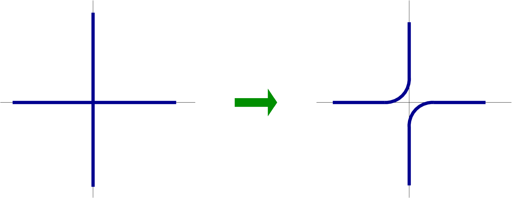
Refer to caption
Figure 2. The rule for splitting four edges meeting at one point into two pairs of linked edges. To obtain the set of contours that separates {x:ϕ⁡(x)≥h}\{x\ :\ \phi(x)\geq h\} from {x:ϕ⁡(x)<h}\{x\ :\ \phi(x)<h\} for h∈ℤh\in{\mathbb{Z}}, we draw all dual edges separating two sites xx, yy such that ϕ⁡(x)≥h>ϕ⁡(y)\phi(x)\geq h>\phi(y) and apply the above graphic rule for every dual vertex where four edges meet. When several sets of level lines include the same contour, it corresponds to a cylinder of intensity 22 or more for ϕ\phi.

We let γ¯\overline{\gamma} denote the set of vertices of ℤ2{\mathbb{Z}}^{2} enclosed by γ~\widetilde{\gamma}. We refer to γ¯\overline{\gamma} as the interior of γ\gamma and say that |γ¯||\overline{\gamma}| is the volume enclosed in the contour γ\gamma. We let Δγ\Delta_{\gamma}, the neighborhood of γ\gamma, be the set of vertices of ℤ2{\mathbb{Z}}^{2} located either at a (Euclidean) distance 1/21/2 from γ~\widetilde{\gamma} (when considered as a subset of ℝ2{\mathbb{R}}^{2}) or at a distance 1/21/\sqrt{2} from the meeting point of two non-linked edges. We split the Δγ\Delta_{\gamma} into two disjoint sets, the internal and the external neighborhoods of γ\gamma (see Figure 3)

Δγ−:=Δγ∩γ¯ and Δγ+:=Δγ∩γ¯∁.\Delta^{-}_{\gamma}:=\Delta_{\gamma}\cap\overline{\gamma}\quad\text{ and }\quad\Delta^{+}_{\gamma}:=\Delta_{\gamma}\cap\overline{\gamma}^{\complement}. (3.1)

Given a finite set Λ⊂ℤ2\Lambda\subset{\mathbb{Z}}^{2} a contour γ\gamma is said to be in Λ\Lambda if γ¯⊂Λ\overline{\gamma}\subset\Lambda. We let 𝒞{\mathcal{C}} denote the set of contours in ℤ2{\mathbb{Z}}^{2} and 𝒞Λ{\mathcal{C}}_{\Lambda} that of contours in Λ\Lambda. Given ϕ∈ΩΛ\phi\in\Omega_{\Lambda}, we say that γ∈𝒞Λ\gamma\in{\mathcal{C}}_{\Lambda} is a contour for ϕ\phi with boundary condition nn, if there exists k≥1k\geq 1 such that

minx∈Δγ−⁡ϕ⁡(x)=maxx∈Δγ+⁡ϕ⁡(x)+k​ε​(γ).\min_{x\in\Delta^{-}_{\gamma}}\phi(x)=\max_{x\in\Delta^{+}_{\gamma}}\phi(x)+k\varepsilon(\gamma). (3.2)

where in the above equation by convention we consider that

ϕ⁡(x)=n if x∈Λ∁.\phi(x)=n\quad\text{ if }\quad x\in\Lambda^{\complement}.

The quantity kk appearing in (3.2) is called the intensity of the contour and the triplet (γ,k)=(γ~,ε⁡(γ),k)(\gamma,k)=(\widetilde{\gamma},\varepsilon(\gamma),k) with γ∈𝒞\gamma\in{\mathcal{C}} and k∈ℕk\in{\mathbb{N}} an intensity, is called a cylinder. We say that (γ,k)(\gamma,k) is a cylinder for ϕ\phi (with boundary condition nn) if γ\gamma is a contour of intensity kk. The cylinder function associated with (γ,k)(\gamma,k) is defined on ℤ2{\mathbb{Z}}^{2} by

φ(γ,k)​(x)=ε⁡(γ)​k​𝟏γ¯​(x).\varphi_{(\gamma,k)}(x)=\varepsilon(\gamma)k\mathbf{1}_{\overline{\gamma}}(x). (3.3)

We use the notation γ^\widehat{\gamma} to denote a generic cylinder and write k⁡(γ^)k(\widehat{\gamma}) to denote its intensity. With some small abuse of notation, γ~\widetilde{\gamma}, γ\gamma and γ¯\overline{\gamma} denote the geometric contour, contour, and contour interior associated with γ^\widehat{\gamma}. We let Υ^n​(ϕ)\widehat{\Upsilon}_{n}(\phi) denote the set of cylinders for ϕ\phi with boundary condition nn and Υn​(ϕ)\Upsilon_{n}(\phi) the corresponding set of contours.

We say that Λ\Lambda is a simply connected subset of ℤ2{\mathbb{Z}}^{2}, if it can be expressed as the interior of a contour, that is, if

∃γΛ∈𝒞,γ¯Λ=Λ.\exists\gamma_{\Lambda}\in{\mathcal{C}},\quad\overline{\gamma}_{\Lambda}=\Lambda. (3.4)

Note that, when Λ\Lambda is simply connected, an element ϕ∈ΩΛ\phi\in\Omega_{\Lambda} is uniquely characterized by its cylinders. More precisely, we have

∀x∈Λ,ϕ⁡(x):=n+∑γ^∈Υ^n​(ϕ)φγ^​(x).\forall x\in\Lambda,\quad\phi(x):=n+\sum_{\widehat{\gamma}\in\widehat{\Upsilon}_{n}(\phi)}\varphi_{\widehat{\gamma}}(x). (3.5)

Furthermore, the reader can check that

ℋΛn​(ϕ)=∑γ^∈Υ^n​(ϕ)k⁡(γ^)​|γ~|.{\mathcal{H}}^{n}_{\Lambda}(\phi)=\sum_{\widehat{\gamma}\in\widehat{\Upsilon}_{n}(\phi)}k(\widehat{\gamma})|\widetilde{\gamma}|. (3.6)

Of course not every set of cylinder is of the form Υ^n​(ϕ)\widehat{\Upsilon}_{n}(\phi) and we must introduce a notion of compatibility which characterizes the “right” sets of cylinder.

Two cylinders γ^\widehat{\gamma} and γ^′\widehat{\gamma}^{\prime} are said to be compatible if they are cylinders for the function φγ^+φγ^′\varphi_{\widehat{\gamma}}+\varphi_{\widehat{\gamma}^{\prime}}. This is equivalent to the three following conditions being satisfied : (see Figure 3)

  • (i)

    γ~≠γ~′\widetilde{\gamma}\neq\widetilde{\gamma}^{\prime} and γ¯∩γ¯′∈{∅,γ¯,γ¯′}\overline{\gamma}\cap\overline{\gamma}^{\prime}\in\{\emptyset,\overline{\gamma},\overline{\gamma}^{\prime}\}.

  • (ii)

    If ε=ε′\varepsilon=\varepsilon^{\prime} and γ¯∩γ¯′=∅\overline{\gamma}\cap\overline{\gamma}^{\prime}=\emptyset, then then γ¯′∩Δγ+=∅\overline{\gamma}^{\prime}\cap\Delta^{+}_{\gamma}=\emptyset .

  • (iii)

    If ε≠ε′\varepsilon\neq\varepsilon^{\prime} and γ¯′⊂γ¯\overline{\gamma}^{\prime}\subset\overline{\gamma} (resp. γ¯⊂γ¯′\overline{\gamma}\subset\overline{\gamma}^{\prime}) then γ¯′∩Δγ−=∅\overline{\gamma}^{\prime}\cap\Delta^{-}_{\gamma}=\emptyset (resp. γ¯∩Δγ′−=∅\overline{\gamma}\cap\Delta^{-}_{\gamma^{\prime}}=\emptyset).

This first condition simply states that compatible contours do not cross each-other. The conditions γ¯′∩Δγ+=∅\overline{\gamma}^{\prime}\cap\Delta^{+}_{\gamma}=\emptyset and γ¯′∩Δγ−=∅\overline{\gamma}^{\prime}\cap\Delta^{-}_{\gamma}=\emptyset in (i​i)(ii) and (i​i​i)(iii) can be reformulated as: γ~\widetilde{\gamma} and γ~′\widetilde{\gamma}^{\prime} do not share edges, and if both γ~\widetilde{\gamma} and γ~′\widetilde{\gamma}^{\prime} possess two edges adjacent to one vertex x∗∈(ℤ2)∗x^{*}\in({\mathbb{Z}}^{2})^{*} then the two edges in γ\gamma are linked and so are those in γ′\gamma^{\prime}.

Refer to caption
Figure 3. A contour γ\gamma represented with its internal (Δγ−\Delta^{-}_{\gamma} circles) and external ( Δγ+\Delta^{+}_{\gamma}, squares) neighborhood. To be compatible with γ\gamma, a contour γ′\gamma^{\prime} of the same sign such that γ¯′∩γ¯=∅\overline{\gamma}^{\prime}\cap\overline{\gamma}=\emptyset cannot enclose any squares. A compatible contour of opposite sign enclosed in γ\gamma (such that γ¯′⊂γ¯\overline{\gamma}^{\prime}\subset\overline{\gamma}) cannot enclose any circles.

Note that the compatibility of two cylinders does not depend on their respective intensity, so that the notion can naturally be extended to signed contours : the contours γ\gamma and γ′\gamma^{\prime} are said to be compatible (we write γ|γ′\gamma\mid\gamma^{\prime}) if the cylinders (γ,1)(\gamma,1) and (γ′,1)(\gamma^{\prime},1) are. Two distinct non-compatible contours are said to be connected (we write γ⟂γ′\gamma\perp\gamma^{\prime}).

Refer to caption
Figure 4. A compatible collection of contour on the dual lattice (the primal lattice is represented in dotted lines). Contours of different signs are displayed in different colors (red-dotted/blue-solid).

A (finite or countable) collection of cylinders (or of signed contours) is said to be a compatible collection if its elements are pairwise compatible (see Figure 4). The reader can check by inspection the following claim which establishes that the set of compatible collections of cylinders is in bijection with ΩΛ\Omega_{\Lambda} (simple connectivity is required to avoid having level lines enclosing holes).

Lemma 3.2.

If Λ\Lambda is simply connected, then for any ϕ∈ΩΛ\phi\in\Omega_{\Lambda}, Υ^n​(ϕ)\widehat{\Upsilon}_{n}(\phi) is a compatible collection of cylinders and reciprocally, if Γ^⊂𝒞^Λ\widehat{\Gamma}\subset\widehat{\mathcal{C}}_{\Lambda} is a compatible collection of cylinder in Λ\Lambda then its elements are the cylinders of the function ∑γ^∈Γ^φγ^.\sum_{\widehat{\gamma}\in\widehat{\Gamma}}\varphi_{\widehat{\gamma}}.

Using (3.6) and the contour representation above, we can rewrite the partition function 𝒵Λ,β{\mathcal{Z}}_{\Lambda,\beta} in a new form. We let 𝒦⁡(Λ){\mathcal{K}}(\Lambda) and 𝒦^​(Λ)\widehat{\mathcal{K}}(\Lambda) denote the set of compatible collections of contour and cylinders in Λ\Lambda. We have

𝒵Λ,β=∑Γ^∈𝒦^​(Λ)∏γ^∈Γ^e−k⁡(γ^)​β​|γ~|.{\mathcal{Z}}_{\Lambda,\beta}=\sum_{\widehat{\Gamma}\in\widehat{\mathcal{K}}(\Lambda)}\prod_{\widehat{\gamma}\in\widehat{\Gamma}}e^{-k(\widehat{\gamma})\beta|\widetilde{\gamma}|}. (3.7)

Summing over all the possible intensities, we obtain

𝒵Λ,β=∑Γ∈𝒦⁡(Λ)∏γ∈Γ1eβ​|γ~|−1.{\mathcal{Z}}_{\Lambda,\beta}=\sum_{\Gamma\in{\mathcal{K}}(\Lambda)}\prod_{\gamma\in\Gamma}\frac{1}{e^{\beta|\widetilde{\gamma}|}-1}. (3.8)

This rewriting of the partition function entails that under 𝐏Λ,β{\mathbf{P}}_{\Lambda,\beta} the distribution of Υn​(ϕ)\Upsilon_{n}(\phi) is a product measure conditioned to compatibility. In particular as the event “being compatible” is a decreasing event for the inclusion relation in the power set 𝒫⁡(𝒞Λ){\mathcal{P}}({\mathcal{C}}_{\Lambda}), Harris inequality [30] implies that 𝐏Λ,β{\mathbf{P}}_{\Lambda,\beta} is stochastically dominated by this product measure. To make this more explicit, let 𝐐Λ,β{\mathbf{Q}}_{\Lambda,\beta} be the distribution of a random element χ∈𝒫⁡(𝒞Λ)\chi\in{\mathcal{P}}({\mathcal{C}}_{\Lambda}) (the power set of 𝒞Λ{\mathcal{C}}_{\Lambda}) under which the variables χ(γ):=𝟏{γ∈χ}\chi(\gamma):=\mathbf{1}_{\{\gamma\in\chi\}} are independent and

𝐐Λ,β​(γ∈χ)=e−β​|γ~|.{\mathbf{Q}}_{\Lambda,\beta}\left(\gamma\in\chi\right)=e^{-\beta|\widetilde{\gamma}|}. (3.9)

We refer to [34, Lemma 4.3 and 4.4] for more details of the proof of the following statement.

Lemma 3.3.

The distribution of the cylinders in Υ^n​(ϕ)\widehat{\Upsilon}_{n}(\phi) can be described as follows:

  • (A)

    We have

    𝐏Λ,βn[Υn(ϕ)∈⋅]:=𝐐Λ,β[χ∈⋅|χ is a compatible collection ].{\mathbf{P}}^{n}_{\Lambda,\beta}[\Upsilon_{n}(\phi)\in\cdot]:={\mathbf{Q}}_{\Lambda,\beta}\left[\chi\in\cdot\ |\ \chi\text{ is a compatible collection }\right]. (3.10)

    In particular the distribution of Υn​(ϕ)\Upsilon_{n}(\phi) is stochastically dominated (for the inclusion) by 𝐐Λ,β{\mathbf{Q}}_{\Lambda,\beta}.

  • (B)

    Conditionned to the realization Υn​(ϕ)\Upsilon_{n}(\phi) the intensities (k⁡(γ^))γ^∈Υ^n​(ϕ)(k(\widehat{\gamma}))_{\widehat{\gamma}\in\widehat{\Upsilon}_{n}(\phi)} are independent geometric variable of parameter e−β​|γ~|e^{-\beta|\widetilde{\gamma}|}

We end up this section by introducing some notation an terminology which we use in the remainder of the paper.

SOS measure with contour restrictions: For a fixed set of contours 𝐋⊂𝒞Λ{\mathbf{L}}\subset{\mathcal{C}}_{\Lambda}, let us define the measure 𝐏𝐋,Λ,βn{\mathbf{P}}^{n}_{{\mathbf{L}},\Lambda,\beta} which is obtained by conditioning all the contours of ϕ\phi to belong to 𝐋{\mathbf{L}}

𝐏𝐋,Λ,βn:=𝐏Λ,βn[⋅|Υn(ϕ)⊂𝐋]{\mathbf{P}}^{n}_{{\mathbf{L}},\Lambda,\beta}:={\mathbf{P}}^{n}_{\Lambda,\beta}\left[\cdot\ |\ \Upsilon_{n}(\phi)\subset{\mathbf{L}}\right] (3.11)

The proof of Lemma 3.3 extends to 𝐏𝐋,Λ,βn{\mathbf{P}}^{n}_{{\mathbf{L}},\Lambda,\beta} in the sense that under the measure 𝐏𝐋,Λ,βn{\mathbf{P}}^{n}_{{\mathbf{L}},\Lambda,\beta}, the distribution of Υn​(ϕ)\Upsilon_{n}(\phi) is stochastically dominated by that of χ∩𝐋\chi\cap{\mathbf{L}} under 𝐐Λ,β{\mathbf{Q}}_{\Lambda,\beta} (and thus also by that of χ\chi). This is because the distribution 𝐏Λ,βn[Υn(ϕ)∈⋅|Υn(ϕ)⊂𝐋]{\mathbf{P}}^{n}_{\Lambda,\beta}\left[\Upsilon_{n}(\phi)\in\cdot\ |\ \Upsilon_{n}(\phi)\subset{\mathbf{L}}\right] is a product distribution on 𝒫⁡(𝐋){\mathcal{P}}({\mathbf{L}}) constrained to a decreasing event for the inclusion in 𝒫⁡(𝐋){\mathcal{P}}({\mathbf{L}}) (compatibility).

External contours: Given Γ\Gamma a compatible collection of contours and γ∈Γ\gamma\in\Gamma, we say that γ\gamma is an external contour in Γ\Gamma if γ¯\overline{\gamma} is maximal in Γ\Gamma for the inclusion (this time we are considering the inclusion relation in ℤ2{\mathbb{Z}}^{2}), that is

∀γ′∈Γ,γ¯′⊂γ¯​ or ​γ¯′∩γ¯=∅.\forall\gamma^{\prime}\in\Gamma,\quad\overline{\gamma}^{\prime}\subset\overline{\gamma}\text{ or }\overline{\gamma}^{\prime}\cap\overline{\gamma}=\emptyset. (3.12)

We let Υnext​(ϕ)\Upsilon^{\mathrm{ext}}_{n}(\phi) denote the set of external contours in Υn​(ϕ)\Upsilon_{n}(\phi). For A⊂ℤdA\subset{\mathbb{Z}}^{d} we let ϕ↾A\phi\!\!\upharpoonright_{A} denote the restriction of ϕ\phi to the set AA. Note that under 𝐏Λ,βn{\mathbf{P}}^{n}_{\Lambda,\beta} (and also under 𝐏𝐋,Λ,βn{\mathbf{P}}^{n}_{{\mathbf{L}},\Lambda,\beta} for arbitrary 𝐋{\mathbf{L}}), conditionned to the realization of Υnext​(ϕ)\Upsilon^{\mathrm{ext}}_{n}(\phi) the restrictions of ϕ\phi to the interior of external contours ϕ↾γ¯\phi\!\!\upharpoonright_{\overline{\gamma}}, γ∈Υnext​(ϕ)\gamma\in\Upsilon^{\mathrm{ext}}_{n}(\phi) are independent.

3.2. Peak probabilities estimates for the SOS measure

We introduce here a result concerning the asymptotic probability of observing high points for ϕ\phi under 𝐏𝐋,Λ,β{\mathbf{P}}_{{\mathbf{L}},\Lambda,\beta}. Having estimates which are also valid with a contour restriction is of crucial importance in our proofs. To state the result, we need to introduce the following notion of distance between a vertex and the complement of a finite set of contours

d⁡(x,𝐋∁):=min⁡{γ∈𝒞∖𝐋,maxy∈γ¯⁡|x−y|}.d(x,{\mathbf{L}}^{\complement}):=\min\{\gamma\in{\mathcal{C}}\setminus{\mathbf{L}},\max_{y\in\overline{\gamma}}|x-y|\}. (3.13)

Note that if 𝐋⊃𝒞Λ{\mathbf{L}}\supset{\mathcal{C}}_{\Lambda} then d⁡(x,𝐋∁)d(x,{\mathbf{L}}^{\complement}) is larger than the distance from xx to Λ∁\Lambda^{\complement}. The following estimates are proved in Appendix B.

Proposition 3.4.

There exists a constant CC such that if β≥β0\beta\geq\beta_{0} sufficiently large, then such for any choice Λ\Lambda, 𝐋{\mathbf{L}}

  • (i)

    For any x∈Λx\in\Lambda for any n≥0n\geq 0 we have

    𝐏𝐋,Λ,β[ϕ(x)≥n]≤Ce−4​β​n.{\mathbf{P}}_{{\mathbf{L}},\Lambda,\beta}[\phi(x)\geq n]\leq Ce^{-4\beta n}. (3.14)

    If in addition, the positive contour of length 44 surrounding xx (which we denote by γx\gamma_{x} is in 𝐋{\mathbf{L}} we have

    𝐏𝐋,Λ,β[ϕ(x)=n]≥C−1e−4​β​n.{\mathbf{P}}_{{\mathbf{L}},\Lambda,\beta}[\phi(x)=n]\geq C^{-1}e^{-4\beta n}. (3.15)
  • (ii)

    For any x,y∈Λx,y\in\Lambda for any n≥0n\geq 0 we have

    𝐏𝐋,Λ,β[min(ϕ(x),ϕ(y))≥n]≤Ce−6​β​n.{\mathbf{P}}_{{\mathbf{L}},\Lambda,\beta}[\min(\phi(x),\phi(y))\geq n]\leq Ce^{-6\beta n}. (3.16)
  • (iii)

    For any x∈Λx\in\Lambda for any n≥0n\geq 0 we have

    |𝐏𝐋,Λ,β[ϕ(x)≥n]−θ1e−4​β​n|≤C(e−6​β​n+e−d⁡(x,𝐋∁)).\left|{\mathbf{P}}_{{\mathbf{L}},\Lambda,\beta}[\phi(x)\geq n]-\theta_{1}e^{-4\beta n}\right|\leq C\left(e^{-6\beta n}+e^{-d(x,{\mathbf{L}}^{\complement})}\right). (3.17)
  • (iv)

    For any x1,…,xkx_{1},\dots,x_{k}, we have for n≥0n\geq 0

    𝐏𝐋,Λ,β[mini∈⟦1,k⟧ϕ(xi)≥n]≤Cke−3​β​k.{\mathbf{P}}_{{\mathbf{L}},\Lambda,\beta}\left[\min_{i\in\llbracket 1,k\rrbracket}\phi(x_{i})\geq n\right]\leq C_{k}e^{-3\beta\sqrt{k}}. (3.18)
Remark 3.5.

Let us discuss here about the requirement on β\beta for our estimates to be valid. The proof of (3.14)-(3.16) and (3.18) are essentially based on a Peierls-type argument [36] and does not require more than the following condition

∑{γ∈𝒞: 0∈γ¯}e−β​|γ~|<∞\sum_{\{\gamma\in{\mathcal{C}}\ :\ {\bf 0\in\overline{\gamma}}\}}e^{-\beta|\widetilde{\gamma}|}<\infty

which is valid when β≥1\beta\geq 1. On the contrary (3.17) requires the convergence of the cluster expansion associated with the contour decomposition which is a more stringent condition. Looking at the discussion in [32, pp 493] and considering that the number of contours of length nn containing 𝟎{\bf 0} is bounded above by n​3n−2≤4nn3^{n-2}\leq 4^{n} and that the weight associated with contours satisfy for β≥1\beta\geq 1,

(eβ​|γ~|−1)−1≤e−9​β10​|γ~|,(e^{\beta|\widetilde{\gamma}|}-1)^{-1}\leq e^{-\frac{9\beta}{10}|\widetilde{\gamma}|},

we obtain that our estimates are valid as long as

β≥109​(log⁡4+1.6).\beta\geq\frac{10}{9}(\log 4+1.6).

Hence in all our statements, β\beta sufficiently large can be replaced by β≥3.5\beta\geq 3.5.

4. Lower bound on the free energy

4.1. Result and decomposition of the proof

The object of this section is to prove a quantitative version of the lower bound part of (2.21).

Proposition 4.1.

There exists ε\varepsilon such that for all β\beta sufficiently large and all α>0\alpha>0, there exists C⁡(α,β)>0C(\alpha,\beta)>0 such that for all h>0h>0

f¯β​(α,h)≥Gβ​(α,h)−C⁡(α,β)​h2+ε.\overline{\textsc{f}}_{\beta}(\alpha,h)\geq G_{\beta}(\alpha,h)-C(\alpha,\beta)h^{2+\varepsilon}. (4.1)

Note that as we have Gβ​(α,h)≍h→0+h2G_{\beta}(\alpha,h)\stackrel{{\scriptstyle h\to 0+}}{{\asymp}}h^{2}, (4.1) implies immediately that

lim infh→0+f¯β​(α,h)Gβ​(α,h)≥1.\liminf_{h\to 0+}\frac{\overline{\textsc{f}}_{\beta}(\alpha,h)}{G_{\beta}(\alpha,h)}\geq 1.

Let us also observe that it is enough to prove the statement for h≤h0​(α,β)h\leq h_{0}(\alpha,\beta) where h0h_{0} can be chosen arbitrarily small. Indeed by tuning the value of C⁡(α,β)C(\alpha,\beta) we can make the r.h.s. of (4.1) negative for all h≥h0h\geq h_{0}. We can make the constant ε\varepsilon in Proposition 4.1 explicit (the reader can check reading through the proof that ε=1/100\varepsilon=1/100 works), but we choose to work with a letter for the sake of readability.

Decomposition of the proof of Proposition 4.1

In this whole section we fix n=nG=nG​(h)n=n_{G}=n_{G}(h) to be the maximizer in (2.22) (there is a geometric sequence of values for hh for which (2.22) admits two maximizers, in the case we select the smallest one). We have

nG​(h)=max⁡(0,⌈log⁡(θ1​(eλ⁡(2​α)−2​λ​(α)−1)/(2​h))4​β⌉)n_{G}(h)=\max\left(0,\left\lceil\frac{\log\left(\theta_{1}(e^{\lambda(2\alpha)-2\lambda(\alpha)}-1)/(2h)\right)}{4\beta}\right\rceil\right) (4.2)

In particular nG​(h)n_{G}(h) is asymptotically equivalent to |log⁡h|/4​β|\log h|/4\beta and as we are interested in the small values of hh, we can think of nn as large. Recalling the definition of the reduced partition function (2.15), we are going to show that for N≥N0​(h)N\geq N_{0}(h) sufficiently large we have

1N2​𝔼​log⁡Zβ,Nn,h,α,ω≥Gβ​(α,β)−C⁡(α,β)​h2+ε.\frac{1}{N^{2}}{\mathbb{E}}\log Z^{n,h,\alpha,\omega}_{\beta,N}\geq G_{\beta}(\alpha,\beta)-C(\alpha,\beta)h^{2+\varepsilon}. (4.3)

Taking the limit of (4.3) when NN tends to infinity we obtain (4.1). We split the proof of the result in two main steps and three lemmas. Our first step get rid of the possibility of having large contours. We show that Zβ,Nn,h,α,ωZ^{n,h,\alpha,\omega}_{\beta,N} can be replaced by

Z~β,Nn,h,α,ω:=𝐄~N,βn​[e∑x∈ΛN(α​ωx−λ⁡(α)+h)​δx],\widetilde{Z}^{n,h,\alpha,\omega}_{\beta,N}:=\widetilde{\mathbf{E}}^{n}_{N,\beta}\left[e^{\sum_{x\in\Lambda_{N}}(\alpha\omega_{x}-\lambda(\alpha)+h)\delta_{x}}\right],

where

𝐏~N,βn:=𝐏N,βn[⋅|𝒜N,n],\widetilde{\mathbf{P}}^{n}_{N,\beta}:={\mathbf{P}}^{n}_{N,\beta}[\cdot\ |\ {\mathcal{A}}_{N,n}],

is the SOS measure with boundary condition nn, conditioned not to display contours of length larger than n4n^{4}.

𝒜N,n:={∀γ∈Υn(ϕ),|γ~|≤n4}.{\mathcal{A}}_{N,n}:=\left\{\forall\gamma\in\Upsilon_{n}(\phi),|\widetilde{\gamma}|\leq n^{4}\right\}.

The choice of n4n^{4} for the threshold defining large contours is quite arbitrary (the only requirements are subexponential growth in nn and being of a larger order of magnitude than n2n^{2}) and but turns out to be convenient in the computation. The following lemma implies that Z~β,Nn,h,α,ω\widetilde{Z}^{n,h,\alpha,\omega}_{\beta,N} is a good approximation for Zβ,Nn,h,α,ωZ^{n,h,\alpha,\omega}_{\beta,N}.

Lemma 4.2.

We have for all β≥2​log⁡3\beta\geq 2\log 3, and all integers NN and nn

𝐏N,βn[𝒜N,n]≥exp(−4e−βn4/2N2).{\mathbf{P}}^{n}_{N,\beta}\left[{\mathcal{A}}_{N,n}\right]\geq\exp\left(-4e^{-\beta n^{4}/2}N^{2}\right). (4.4)

In particular we have

logZn,h,α,ωβ,N≥logZ~n,h,α,ωβ,N−4N2e−βn4/2.\log Z^{n,h,\alpha,\omega}_{\beta,N}\geq\log\widetilde{Z}^{n,h,\alpha,\omega}_{\beta,N}-4N^{2}e^{-\beta n^{4}/2}. (4.5)

Note that with our choice for n=nG​(h)n=n_{G}(h), we have 4e−βnG4/2≤h34e^{-\beta n_{G}^{4}/2}\leq h^{3} for hh sufficiently small and thus it is sufficient to prove (4.3) with Zβ,Nn,h,α,ωZ^{n,h,\alpha,\omega}_{\beta,N} replaced by Z~β,Nn,h,α,ω\widetilde{Z}^{n,h,\alpha,\omega}_{\beta,N}. The second step is more delicate and relies on a coarse graining argument. We wish to divide our system into cells in order to factorize the partition function. In order to obtain a factorization we must condition on the realization of the set of contours which intersect several cells.

We set M=h−150M=h^{-\frac{1}{50}}, N=k​MN=kM where k∈ℕk\in{\mathbb{N}} is arbitrary. Imposing that NN is a multiple of NN is by no mean restrictive. Indeed, since the limit of the l.h.s. exists, it is in fact sufficient to prove (4.3) along a subsequence. We divide ΛN=⟦1,N⟧\Lambda_{N}=\llbracket 1,N\rrbracket in k2k^{2} boxes. We let

ℍ=ℍM:={(x1,x2)∈(ℤ2)∗:M​|(x1−1/2)​ or ​M|​(x2−1/2)}{\mathbb{H}}={\mathbb{H}}_{M}:=\{(x_{1},x_{2})\in({\mathbb{Z}}^{2})^{*}\ :\ M|(x_{1}-1/2)\text{ or }M|(x_{2}-1/2)\}

denote the grid in the dual lattice which splits ΛN\Lambda_{N} into cells of side-length MM. We index these cells by z∈⟦0,k−1⟧2z\in\llbracket 0,k-1\rrbracket^{2}, and set 𝒞z:=ΛM+M​z{\mathcal{C}}_{z}:=\Lambda_{M}+Mz. Recalling the definition of an external contour (3.12), we are going to consider the set of countours intersecting ℍ{\mathbb{H}} (here we consider the vertex intersection)

U⁡(ϕ):={γ∈Υnext​(ϕ):γ∩ℍ≠∅}.U(\phi):=\{\gamma\in\Upsilon_{n}^{\mathrm{ext}}(\phi)\ :\ \gamma\cap{\mathbb{H}}\neq\emptyset\}.

Note that the contours of U⁡(ϕ)U(\phi) naturally provides a partition of the box ΛN\Lambda_{N}. If U⁡(ϕ)=ΓU(\phi)=\Gamma, setting Γ¯:=⋃γ∈Γγ¯\overline{\Gamma}:=\bigcup_{\gamma\in\Gamma}\overline{\gamma}, we let, for z∈⟦0,k−1⟧2z\in\llbracket 0,k-1\rrbracket^{2}, ℬz{\mathcal{B}}_{z} denote the set of sites in 𝒞z{\mathcal{C}}_{z} which are not enclosed in a contour of Γ\Gamma,

ℬz:=𝒞z∖Γ¯.{\mathcal{B}}_{z}:={\mathcal{C}}_{z}\setminus\overline{\Gamma}.

Note that ℬz{\mathcal{B}}_{z} is not necessarily connected. We can observe that

ΛN=(⋃z∈⟦1,k⟧ℬz)∪(⋃γ∈Γγ¯),\Lambda_{N}=\left(\bigcup_{z\in\llbracket 1,k\rrbracket}{\mathcal{B}}_{z}\right)\cup\left(\bigcup_{\gamma\in\Gamma}\overline{\gamma}\right), (4.6)

and that the union is disjoint. Moreover using the contour decomposition, one can check that conditioned on U⁡(ϕ)=ΓU(\phi)=\Gamma, the restrictions of ϕ\phi to the regions of the partition in the l.h.s. of (4.6) form an independent family. Hence we have

𝐄~N,βn​[e∑x∈ΛN(α​ωx−λ⁡(α)+h)​δx|U⁡(ϕ)=Γ]=∏z∈⟦0,k−1⟧2𝐄~nN,β[e∑x∈ℬz(α​ωx−λ⁡(α)+h)​δx|U(ϕ)=Γ]×∏γ∈Γ𝐄~N,βn​[e∑x∈γ¯(α​ωx−λ⁡(α)+h)​δx|U⁡(ϕ)=Γ],\widetilde{\mathbf{E}}^{n}_{N,\beta}\left[e^{\sum_{x\in\Lambda_{N}}(\alpha\omega_{x}-\lambda(\alpha)+h)\delta_{x}}|U(\phi)=\Gamma\right]\\ =\prod_{z\in\llbracket 0,k-1\rrbracket^{2}}\widetilde{\mathbf{E}}^{n}_{N,\beta}\left[e^{\sum_{x\in{\mathcal{B}}_{z}}(\alpha\omega_{x}-\lambda(\alpha)+h)\delta_{x}}\ |\ U(\phi)=\Gamma\right]\\ \times\prod_{\gamma\in\Gamma}\widetilde{\mathbf{E}}^{n}_{N,\beta}\left[e^{\sum_{x\in\overline{\gamma}}(\alpha\omega_{x}-\lambda(\alpha)+h)\delta_{x}}\ |\ U(\phi)=\Gamma\right], (4.7)

and as a consequence

𝔼logZ~n,h,α,ωβ,N≥minΓ[∑z∈⟦0,k−1⟧2𝔼log𝐄~nN,β[e∑x∈ℬz(α​ωx−λ⁡(α)+h)​δz|U(ϕ)=Γ]+∑γ∈Γ𝔼log𝐄~nN,β[e∑x∈γ¯(α​ωx−λ⁡(α)+h)​δz|U(ϕ)=Γ]],{\mathbb{E}}\log\widetilde{Z}^{n,h,\alpha,\omega}_{\beta,N}\geq\min_{\Gamma}\Bigg[\sum_{z\in\llbracket 0,k-1\rrbracket^{2}}{\mathbb{E}}\log\widetilde{\mathbf{E}}^{n}_{N,\beta}\left[e^{\sum_{x\in{\mathcal{B}}_{z}}(\alpha\omega_{x}-\lambda(\alpha)+h)\delta_{z}}\ |\ U(\phi)=\Gamma\right]\\ +\sum_{\gamma\in\Gamma}{\mathbb{E}}\log\widetilde{\mathbf{E}}^{n}_{N,\beta}\left[e^{\sum_{x\in\overline{\gamma}}(\alpha\omega_{x}-\lambda(\alpha)+h)\delta_{z}}\ |\ U(\phi)=\Gamma\right]\Bigg], (4.8)

where the minimum is taken over all possible realization of U⁡(ϕ)U(\phi). To conclude we obtain a lower bound on each term of the two sums in the l.h.s. above, yielding an estimate which is uniform in the realization of U⁡(ϕ)U(\phi). As the cells ℬz{\mathcal{B}}_{z} cover much more area than the interior of contours in U⁡(ϕ)U(\phi), we need to show that sites inside ℬz{\mathcal{B}}_{z} gives a contribution per site very close to Gβ​(α,h)G_{\beta}(\alpha,h), while for the restriction to γ¯\overline{\gamma}, showing that the contribution of each site is of order h2h^{2} in absolute value is sufficient. This the content of the two following lemmas.

Lemma 4.3.

There exists a constant C⁡(α,β)C(\alpha,\beta) such that for any h∈(0,1]h\in(0,1], for any γ∈𝒞ΛN\gamma\in{\mathcal{C}}_{\Lambda_{N}} with |γ~|≤(nG​(h))4|\widetilde{\gamma}|\leq(n_{G}(h))^{4} we have

𝔼​log⁡𝐄~N,βn​[e∑x∈γ¯(α​ωx−λ⁡(α)+h)​δz|γ∈Υnext​(ϕ)]≥−C​|γ¯|​h2.{\mathbb{E}}\log\widetilde{\mathbf{E}}^{n}_{N,\beta}\left[e^{\sum_{x\in\overline{\gamma}}(\alpha\omega_{x}-\lambda(\alpha)+h)\delta_{z}}\ |\ \gamma\in\Upsilon_{n}^{\mathrm{ext}}(\phi)\right]\geq-C|\overline{\gamma}|h^{2}. (4.9)
Lemma 4.4.

There exists a constant h0​(α,β)>0h_{0}(\alpha,\beta)>0 such that if h∈(0,h0​(α,β)]h\in(0,h_{0}(\alpha,\beta)] then we have, for any possible realization of U⁡(ϕ)U(\phi) and any z∈⟦0,k−1⟧z\in\llbracket 0,k-1\rrbracket

𝔼​log⁡𝐄~N,βn​[e∑x∈ℬz(α​ωx−λ⁡(α)+h)​δx|U⁡(ϕ)=Γ]≥M2​[Gβ​(α,h)−h2+ε].{\mathbb{E}}\log\widetilde{\mathbf{E}}^{n}_{N,\beta}\left[e^{\sum_{x\in{\mathcal{B}}_{z}}(\alpha\omega_{x}-\lambda(\alpha)+h)\delta_{x}}\ |\ U(\phi)=\Gamma\right]\geq M^{2}\left[G_{\beta}(\alpha,h)-h^{2+\varepsilon}\right]. (4.10)

Before proving the above results, let us show how they permit to conclude our proof of Proposition 4.1.

Proof of Proposition 4.1.

In view of (4.3),(4.5) and (4.8), we only need to show that for every choice of Γ\Gamma we have

∑z∈⟦0,k−1⟧2𝔼log𝐄~nN,β[e∑x∈ℬz(α​ωx−λ⁡(α)+h)​δz|U(ϕ)=Γ]+∑γ∈Γ𝔼log𝐄~nN,β[e∑x∈γ¯(α​ωx−λ⁡(α)+h)​δz|U(ϕ)=Γ]≥N2​Gβ​(α,h)−C​h2+ε.\sum_{z\in\llbracket 0,k-1\rrbracket^{2}}{\mathbb{E}}\log\widetilde{\mathbf{E}}^{n}_{N,\beta}\left[e^{\sum_{x\in{\mathcal{B}}_{z}}(\alpha\omega_{x}-\lambda(\alpha)+h)\delta_{z}}\ |\ U(\phi)=\Gamma\right]\\ +\sum_{\gamma\in\Gamma}{\mathbb{E}}\log\widetilde{\mathbf{E}}^{n}_{N,\beta}\left[e^{\sum_{x\in\overline{\gamma}}(\alpha\omega_{x}-\lambda(\alpha)+h)\delta_{z}}\ |\ U(\phi)=\Gamma\right]\\ \geq N^{2}G_{\beta}(\alpha,h)-Ch^{2+\varepsilon}. (4.11)

It is a direct consequence of the contours construction that

𝐄~N,βn​[e∑x∈γ¯(α​ωx−λ⁡(α)+h)​δx|U⁡(ϕ)=Γ]=𝐄~N,βn​[e∑x∈γ¯(α​ωx−λ⁡(α)+h)​δx|γ∈Υnext​(ϕ)].\widetilde{\mathbf{E}}^{n}_{N,\beta}\left[e^{\sum\limits_{x\in\overline{\gamma}}(\alpha\omega_{x}-\lambda(\alpha)+h)\delta_{x}}\ |\ U(\phi)=\Gamma\right]=\widetilde{\mathbf{E}}^{n}_{N,\beta}\left[e^{\sum\limits_{x\in\overline{\gamma}}(\alpha\omega_{x}-\lambda(\alpha)+h)\delta_{x}}\ |\ \gamma\in\Upsilon_{n}^{\mathrm{ext}}(\phi)\right]. (4.12)

Hence taking the expectation with respect to ω\omega in (4.8) and using the lemmas to evaluate each term of the sum we obtain that the r.h.s. of (4.11) is larger than

N2​[Gβ​(α,h)−h2+ε]−C​h2​𝐄~N,βn​∑γ∈Γ|γ¯|.N^{2}\left[G_{\beta}(\alpha,h)-h^{2+\varepsilon}\right]-Ch^{2}\widetilde{\mathbf{E}}^{n}_{N,\beta}\sum_{\gamma\in\Gamma}|\overline{\gamma}|. (4.13)

Now the sites enclosed by some γ∈U⁡(ϕ)\gamma\in U(\phi) are all located at distance n4n^{4} from ℍ{\mathbb{H}}. Hence we have (provided that ε<1/50\varepsilon<1/50), for all hh sufficiently small

∑γ∈U⁡(ϕ)|γ¯|≤4​n4​k2​M=4​n4​N2M≤N2​hε.\sum_{\gamma\in U(\phi)}|\overline{\gamma}|\leq 4n^{4}k^{2}M=\frac{4n^{4}N^{2}}{M}\leq N^{2}h^{\varepsilon}.

This is sufficient to conclude.

∎

4.2. Proof of Lemma 4.2

The event 𝒜N,n{\mathcal{A}}_{N,n} is decreasing for the inclusion. Thus applying Lemma 3.3 we have

𝐏N,βn[𝒜N,n]≥𝐐N,β[∀γ∈χ,|γ~|≤n4].{\mathbf{P}}^{n}_{N,\beta}\left[{\mathcal{A}}_{N,n}\right]\geq{\mathbf{Q}}_{N,\beta}[\ \forall\gamma\in\chi,\ |\widetilde{\gamma}|\leq n^{4}]. (4.14)

Now, if 𝒞N{\mathcal{C}}_{N} denotes the set of contours in the box ΛN\Lambda_{N} the latter probability is exactly equal to

∏γ∈𝒞N(1−e−β​|γ~|)≥exp(−2∑γ∈𝒞Ne−β​|γ~|)\prod_{\gamma\in{\mathcal{C}}_{N}}(1-e^{-\beta|\widetilde{\gamma}|})\geq\exp\left(-2\sum_{\gamma\in{\mathcal{C}}_{N}}e^{-\beta|\widetilde{\gamma}|}\right) (4.15)

where we used 1−x≥e−2​x1-x\geq e^{-2x} which is valid for x∈(0,1/2)x\in(0,1/2). We conclude by observing that, as the number contour of length mm in ⟦1,N⟧2\llbracket 1,N\rrbracket^{2} is bounded above by N2​3mN^{2}3^{m}

∑γ∈𝒞Ne−β​|γ~|≤N2​e−(β−log⁡3)​n41−e−(β−log⁡3),\sum_{\gamma\in{\mathcal{C}}_{N}}e^{-\beta|\widetilde{\gamma}|}\leq N^{2}\frac{e^{-(\beta-\log 3)n^{4}}}{1-e^{-(\beta-\log 3)}}, (4.16)

which allows to conclude.

∎

4.3. Proof of Lemma 4.3

For both Lemma 4.3 and 4.4 our strategy is to rely on second moment computation together with a Taylor expansion. Let us first describe the distribution of ϕ\phi restricted to γ¯\overline{\gamma} after the conditioning. We have (recalling (3.1)) from Lemma 3.3

𝐏~N,βn[ϕ↾γ¯∈⋅|γ∈Υnext]={𝐏~n−1γ¯,β[⋅|∀x∈Δγ−,ϕ≤n−1] if ε(γ)=−1,𝐏~n+1γ¯,β[⋅|∀x∈Δγ−,ϕ≥n+1] if ε(γ)=+1.\widetilde{\mathbf{P}}^{n}_{N,\beta}\left[\phi\!\!\upharpoonright_{\overline{\gamma}}\in\cdot|\ \gamma\in\Upsilon^{\mathrm{ext}}_{n}\right]=\begin{cases}\widetilde{\mathbf{P}}^{n-1}_{\overline{\gamma},\beta}[\cdot\ |\ \forall x\in\Delta_{\gamma}^{-},\phi\leq n-1]\quad\text{ if }\varepsilon(\gamma)=-1,\\ \widetilde{\mathbf{P}}^{n+1}_{\overline{\gamma},\beta}[\cdot\ |\ \forall x\in\Delta_{\gamma}^{-},\phi\geq n+1]\quad\text{ if }\varepsilon(\gamma)=+1.\end{cases} (4.17)

where the tilde on the r.h.s. is present to remind ourselves that we are conditioning on having no contour of length more than n4n^{4}. In order to have a better control on the second moment of the partition function, we restrict the computation to the set of surfaces ϕ\phi which display only a small number of contacts. We introduce the event

𝒟γκ:={ϕ:∑x∈γ¯δx≤κ}.{\mathcal{D}}^{\kappa}_{\gamma}:=\{\phi\ :\ \sum_{x\in\overline{\gamma}}\delta_{x}\leq\kappa\}. (4.18)

We fix the value of κ\kappa equal to 100100 (and drop the dependence in κ\kappa in the notation) but keep the letter κ\kappa in the computation for better readability. As in both cases in the r.h.s. of (4.17), the measure is of the type 𝐏𝐋,Λ,βn±1{\mathbf{P}}^{n\pm 1}_{{\mathbf{L}},\Lambda,\beta} (the conditioning corresponds to prohibiting positive (if ε⁡(γ)=−1\varepsilon(\gamma)=-1) or negative (if ε⁡(γ)=+1\varepsilon(\gamma)=+1) contours which enclose elements of Δγ−\Delta^{-}_{\gamma}). Hence using Proposition 3.4 and a union bound we have (recall that |γ¯|≤n16|\overline{\gamma}|\leq n^{16} from the restriction on the contours’ length)

𝐏~N,βn​[𝒟γ∁|γ∈Υext]≤(|γ¯|κ)​e−30​β​(n−1)≤h3,\widetilde{\mathbf{P}}^{n}_{N,\beta}\left[{\mathcal{D}}_{\gamma}^{\complement}\ |\ \gamma\in\Upsilon^{\mathrm{ext}}\right]\leq\binom{|\overline{\gamma}|}{\kappa}e^{-30\beta(n-1)}\leq h^{3}, (4.19)

We define μγ,h\mu_{\gamma,h} the probability on ΩN\Omega_{N} defined by

μγ,h​(A):=𝐄~N,βn​[𝟏𝒟γ∩A​eh​∑x∈γ¯δx|γ∈Υext]𝐄~N,βn​[eh​∑x∈γ¯δx​𝟏𝒟γ|γ∈Υext].\mu_{\gamma,h}(A):=\frac{\widetilde{\mathbf{E}}^{n}_{N,\beta}\left[\mathbf{1}_{{\mathcal{D}}_{\gamma}\cap A}e^{h\sum_{x\in\overline{\gamma}}\delta_{x}}\ |\ \gamma\in\Upsilon^{\mathrm{ext}}\right]}{\widetilde{\mathbf{E}}^{n}_{N,\beta}\left[e^{h\sum_{x\in\overline{\gamma}}\delta_{x}}\mathbf{1}_{{\mathcal{D}}_{\gamma}}\ |\ \gamma\in\Upsilon^{\mathrm{ext}}\right]}. (4.20)

We have

log⁡𝐄~N,βn​[e∑x∈γ¯(α​ωx−λ⁡(α)+h)​δx​𝟏𝒟γ|γ∈Υext]=log⁡𝐄~N,βn​[e∑x∈γ¯h​δx​𝟏𝒟γ|γ∈Υext]+log⁡μγ,h​(e∑x∈γ¯(α​ωx−λ⁡(α))​δx).\log\widetilde{\mathbf{E}}^{n}_{N,\beta}\left[e^{\sum_{x\in\overline{\gamma}}(\alpha\omega_{x}-\lambda(\alpha)+h)\delta_{x}}\mathbf{1}_{{\mathcal{D}}_{\gamma}}\ |\ \gamma\in\Upsilon^{\mathrm{ext}}\right]\\ =\log\widetilde{\mathbf{E}}^{n}_{N,\beta}\left[e^{\sum_{x\in\overline{\gamma}}h\delta_{x}}\mathbf{1}_{{\mathcal{D}}_{\gamma}}\ |\ \gamma\in\Upsilon^{\mathrm{ext}}\right]+\log\mu_{\gamma,h}\left(e^{\sum_{x\in\overline{\gamma}}\left(\alpha\omega_{x}-\lambda(\alpha)\right)\delta_{x}}\right). (4.21)

Using (4.19), when hh is sufficiently small the first term is larger than

log⁡𝐏~N,βn​[𝒟γ|γ∈Υext]≥−h3.\log\widetilde{\mathbf{P}}^{n}_{N,\beta}\left[{\mathcal{D}}_{\gamma}\ |\ \gamma\in\Upsilon^{\mathrm{ext}}\right]\geq-h^{3}.

Now we have to estimate the expectation of the second term. Combining (4.17) with Proposition 3.4 we obtain that for all x∈γ¯x\in\overline{\gamma},

𝐄N,βn​[δx|γ∈Υext]≤C​e−4​β​(n−1),{\mathbf{E}}^{n}_{N,\beta}\left[\delta_{x}\ |\ \gamma\in\Upsilon^{\mathrm{ext}}\right]\leq Ce^{-4\beta(n-1)}, (4.22)

for some positive constant CC. Using the expression for the density and the assumption that |γ¯|≤n16≤C​|log⁡h|16|\overline{\gamma}|\leq n^{16}\leq C|\log h|^{16} we obtain for sufficiently small hh, a similar estimate under μγ,h\mu_{\gamma,h}

μγ,h​(δx)≤C​e−4​β​(n−1)+h​|γ¯|𝐏~N,βn​[𝒟γ|γ∈Υext]≤C′​e−4​β​(n−1).\mu_{\gamma,h}(\delta_{x})\leq\frac{Ce^{-4\beta(n-1)+h|\overline{\gamma}|}}{\widetilde{\mathbf{P}}^{n}_{N,\beta}\left[{\mathcal{D}}_{\gamma}\ |\ \gamma\in\Upsilon^{\mathrm{ext}}\right]}\leq C^{\prime}e^{-4\beta(n-1)}. (4.23)

Then by Markov’s inequality we have

μγ,h​(e∑x∈γ¯(α​ωx−λ⁡(α))​δx)≥μγ,h​(∑x∈γ¯δx=0)≥1−C′​|γ¯|​e−4​β​(n−1)≥12.\mu_{\gamma,h}\left(e^{\sum_{x\in\overline{\gamma}}(\alpha\omega_{x}-\lambda(\alpha))\delta_{x}}\right)\geq\mu_{\gamma,h}\left(\sum_{x\in\overline{\gamma}}\delta_{x}=0\right)\geq 1-C^{\prime}|\overline{\gamma}|e^{-4\beta(n-1)}\geq\frac{1}{2}. (4.24)

We can use the inequality log⁡x≥(x−1)−(x−1)2\log x\geq(x-1)-(x-1)^{2} (valid for x≥1/2x\geq 1/2) and obtain

𝔼⁡[log⁡μγ,h​(e∑x∈γ¯(α​ωx−λ⁡(α))​δx)]≥−𝔼⁡[μγ,h​(e∑x∈γ¯α​ωx−λ⁡(α)−1)2].{\mathbb{E}}\left[\log\mu_{\gamma,h}\left(e^{\sum_{x\in\overline{\gamma}}(\alpha\omega_{x}-\lambda(\alpha))\delta_{x}}\right)\right]\geq-{\mathbb{E}}\left[\mu_{\gamma,h}\left(e^{\sum_{x\in\overline{\gamma}}\alpha\omega_{x}-\lambda(\alpha)}-1\right)^{2}\right]. (4.25)

The average w.r.t. ω\omega can be computed explicitly, we obtain

𝔼⁡[μγ,h​(e∑x∈γ¯α​ωx−λ⁡(α)−1)2]=μγ,h⊗2​[e[λ⁡(2​α)−2​λ​(α)]​∑x∈γ¯δx(1)​δx(2)]−1.{\mathbb{E}}\left[\mu_{\gamma,h}\left(e^{\sum_{x\in\overline{\gamma}}\alpha\omega_{x}-\lambda(\alpha)}-1\right)^{2}\right]=\mu_{\gamma,h}^{\otimes 2}\left[e^{[\lambda(2\alpha)-2\lambda(\alpha)]\sum_{x\in\overline{\gamma}}\delta^{(1)}_{x}\delta^{(2)}_{x}}\right]-1. (4.26)

From the definition of μγ,h\mu_{\gamma,h} we have ∑x∈γ¯δx(1)​δx(2)≤κ\sum_{x\in\overline{\gamma}}\delta^{(1)}_{x}\delta^{(2)}_{x}\leq\kappa, with probability 11. Hence using the fact that for any u∈[0,κ⁡(λ⁡(2​α)−2​λ​(α))]u\in[0,\kappa(\lambda(2\alpha)-2\lambda(\alpha))] we have

eu−1≤u​eκ⁡(λ⁡(2​α)−2​λ​(α)).e^{u}-1\leq ue^{\kappa(\lambda(2\alpha)-2\lambda(\alpha))}. (4.27)

Using (4.23) and the expression for n=nG​(h)n=n_{G}(h) given in (4.2), we can conclude the proof as follows

μγ,h⊗2​[e[λ⁡(2​α)−2​λ​(α)]​∑x∈γ¯δx(1)​δx(2)]−1≤eκ⁡(λ⁡(2​α)−2​λ​(α))​μγ,h⊗2​(∑x∈γ¯δx(1)​δx(2))≤4​eκ⁡(λ⁡(2​α)−2​λ​(α))|γ¯|e−8​β​(n−1)≤C⁡(α,κ,β)​|γ¯|​h2.\mu_{\gamma,h}^{\otimes 2}\left[e^{[\lambda(2\alpha)-2\lambda(\alpha)]\sum_{x\in\overline{\gamma}}\delta^{(1)}_{x}\delta^{(2)}_{x}}\right]-1\leq e^{\kappa(\lambda(2\alpha)-2\lambda(\alpha))}\mu_{\gamma,h}^{\otimes 2}\left(\sum_{x\in\overline{\gamma}}\delta^{(1)}_{x}\delta^{(2)}_{x}\right)\\ \leq 4e^{\kappa(\lambda(2\alpha)-2\lambda(\alpha))}|\overline{\gamma}|e^{-8\beta(n-1)}\leq C(\alpha,\kappa,\beta)|\overline{\gamma}|h^{2}. (4.28)

∎

4.4. Proof of Lemma 4.4

The proof follows the same steps as that of Lemma 4.3, except that we must aim for sharper estimates. We define μ~z,h\widetilde{\mu}_{z,h} a probability of ΩN\Omega_{N} by

μ~z,h​(A):=𝐄~nN,β[𝟏{ϕ↾ℬz∈A∩𝒟z}eh​∑x∈ℬzδx|U(ϕ)=Γ]𝐄~nN,β[𝟏{ϕ↾ℬz∈𝒟z}eh​∑x∈ℬzδx|U(ϕ)=Γ]\widetilde{\mu}_{z,h}(A):=\frac{\widetilde{\mathbf{E}}^{n}_{N,\beta}\left[\mathbf{1}_{\{\phi\ \!\!\upharpoonright_{{\mathcal{B}}_{z}}\in A\cap{\mathcal{D}}_{z}\}}e^{h\sum_{x\in{\mathcal{B}}_{z}}\delta_{x}}\ |\ U(\phi)=\Gamma\right]}{\widetilde{\mathbf{E}}^{n}_{N,\beta}\left[\mathbf{1}_{\{\phi\ \!\!\upharpoonright_{{\mathcal{B}}_{z}}\in{\mathcal{D}}_{z}\}}e^{h\sum_{x\in{\mathcal{B}}_{z}}\delta_{x}}\ |\ U(\phi)=\Gamma\right]} (4.29)

with (again κ\kappa is set to be equal to 100100 but the letter is kept in the computation for better readability)

𝒟z:={ϕ:∑x∈ℬzδx≤κ}.{\mathcal{D}}_{z}:=\{\phi\ :\ \sum_{x\in{\mathcal{B}}_{z}}\delta_{x}\leq\kappa\}. (4.30)

We are going to refine second moment argument of the second section. In particular we want to use the fact (cf. Proposition 3.4) that the probability of contact is close to θ1​e−4​β​n\theta_{1}e^{-4\beta n} for most points inside ℬz{\mathcal{B}}_{z}. As these estimates are not valid close to the boundary of ℬz{\mathcal{B}}_{z}, let us define ℬz′{\mathcal{B}}^{\prime}_{z} a subset of ℬz{\mathcal{B}}_{z} which includes only points in the bulk

ℬz′:=⟦n4,M−n4⟧2+Mz⊂ℬz.{\mathcal{B}}^{\prime}_{z}:=\llbracket n^{4},M-n^{4}\rrbracket^{2}+Mz\subset{\mathcal{B}}_{z}.

The point here is that from the definition, because contours in Γ\Gamma are all of diameter smaller than n4/2n^{4}/2 (length smaller than n4n^{4}) then all points in ℬz′{\mathcal{B}}^{\prime}_{z} are at a distance at least n4/2n^{4}/2 from the boundary of ℬz{\mathcal{B}}_{z}. The following estimates are easily deduced from Proposition 3.4 (we include details at the end of the present subsection).

Lemma 4.5.

There exists constants C>0C>0 and β0>0\beta_{0}>0 such that for all β>β0\beta>\beta_{0} we have

  • (i)

    For all x∈ℬz′x\in{\mathcal{B}}^{\prime}_{z} we have

    |μ~z,h​(δx)−θ1​e−4​β​n|≤C​h3/2.|\widetilde{\mu}_{z,h}(\delta_{x})-\theta_{1}e^{-4\beta n}|\leq Ch^{3/2}. (4.31)

    This estimate is also valid for μ~z,0\widetilde{\mu}_{z,0}.

  • (ii)

    For all x∈ℬzx\in{\mathcal{B}}_{z} we have

    μ~z,h​(δx)≤C​e−4​β​n.\widetilde{\mu}_{z,h}(\delta_{x})\leq Ce^{-4\beta n}. (4.32)

    This is also valid for μ~z,0\widetilde{\mu}_{z,0}.

  • (iii)

    For all x,y∈ℬzx,y\in{\mathcal{B}}_{z}

    μ~z,h​(δx​δy)≤C​e−6​β​n.\widetilde{\mu}_{z,h}(\delta_{x}\delta_{y})\leq Ce^{-6\beta n}. (4.33)

Let us now prove the result using the estimates above. Note that we have

log⁡𝐄~N,βn​[𝟏𝒟z​e∑x∈ℬz(α​ωx−λ⁡(α)+h)​δx|U⁡(ϕ)=Γ]=log⁡𝐄~N,βn​[𝟏𝒟z​e∑x∈ℬzh​δx|U⁡(ϕ)=Γ]+log⁡μ~z,h​(e∑x∈ℬz(α​ωx−λ⁡(α))).\log\widetilde{\mathbf{E}}^{n}_{N,\beta}\left[\mathbf{1}_{{\mathcal{D}}_{z}}e^{\sum_{x\in{\mathcal{B}}_{z}}(\alpha\omega_{x}-\lambda(\alpha)+h)\delta_{x}}\ |\ U(\phi)=\Gamma\right]\\ =\log\widetilde{\mathbf{E}}^{n}_{N,\beta}\left[\mathbf{1}_{{\mathcal{D}}_{z}}e^{\sum_{x\in{\mathcal{B}}_{z}}h\delta_{x}}\ |\ U(\phi)=\Gamma\right]+\log\widetilde{\mu}_{z,h}\left(e^{\sum_{x\in{\mathcal{B}}_{z}}(\alpha\omega_{x}-\lambda(\alpha))}\right). (4.34)

The first term is equal to

log⁡𝐏~N,βn​[𝒟z|U⁡(ϕ)=Γ]+log⁡μ~z,0​(e∑x∈ℬzh​δx).\log\widetilde{\mathbf{P}}^{n}_{N,\beta}\left[{\mathcal{D}}_{z}\ |\ U(\phi)=\Gamma\right]+\log\widetilde{\mu}_{z,0}(e^{\sum_{x\in{\mathcal{B}}_{z}}h\delta_{x}}). (4.35)

Similarly to (4.19) using that M=h−150M=h^{-\frac{1}{50}} and recalling that κ=100\kappa=100, we have

𝐏~N,βn​[𝒟z∁|U⁡(ϕ)=Γ]≤C​(M2κ)​e−30​β​n≤h3/2.\widetilde{\mathbf{P}}^{n}_{N,\beta}\left[{\mathcal{D}}^{\complement}_{z}\ |\ U(\phi)=\Gamma\right]\leq C\binom{M^{2}}{\kappa}e^{-30\beta n}\leq h^{3}/2. (4.36)

Hence the first term in (4.35) is larger than −h3-h^{3}. The second term is larger (by Jensen’s inequality) than

μ~z,0​(∑x∈ℬz′δx)≥(M−2​n2)2​(θ1​h2−C​h5/2)≥M2​(θ1​h2−h2+ε)\widetilde{\mu}_{z,0}\left(\sum_{x\in{\mathcal{B}}^{\prime}_{z}}\delta_{x}\right)\geq(M-2n^{2})^{2}(\theta_{1}h^{2}-Ch^{5/2})\geq M^{2}\left(\theta_{1}h^{2}-h^{2+\varepsilon}\right) (4.37)

where the first inequality is a consequence of (4.31) and the second one follows if from the fact that nn is of order |log⁡h||\log h| and M=h−1/50M=h^{-1/50} (assuming that ε<1/50\varepsilon<1/50). Now concerning the second term in (4.34), we note that using (4.32) and our choice of parameter we have

μ~z,h​(e∑x∈ℬz(α​ωx−λ⁡(α)))≥μ~z,h​(∑x∈ℬzδx=0)≥1−C​e−4​β​n​|ℬz|≥1−h.\widetilde{\mu}_{z,h}(e^{\sum_{x\in{\mathcal{B}}_{z}}(\alpha\omega_{x}-\lambda(\alpha))})\geq\widetilde{\mu}_{z,h}\left(\sum_{x\in{\mathcal{B}}_{z}}\delta_{x}=0\right)\geq{1-Ce^{-4\beta n}|{\mathcal{B}}_{z}|}\geq 1-\sqrt{h}. (4.38)

Hence using the inequality

log⁡x≥(x−1)+12​y2​(x−1)2\log x\geq(x-1)+\frac{1}{2y^{2}}(x-1)^{2}

valid for all x≥yx\geq y we obtain that

𝔼⁡[log⁡μ~z,h​(e∑x∈ℬz(α​ωx−λ⁡(α)))]≥𝔼⁡[μ~z,h​(e∑x∈ℬz(α​ωx−λ⁡(α))−1)]+𝔼⁡[μ~z,h​(e∑x∈ℬz(α​ωx−λ⁡(α))−1)2]2​(1−h)2.{\mathbb{E}}\left[\log\widetilde{\mu}_{z,h}(e^{\sum_{x\in{\mathcal{B}}_{z}}(\alpha\omega_{x}-\lambda(\alpha))})\right]\\ \geq{\mathbb{E}}\left[\widetilde{\mu}_{z,h}(e^{\sum_{x\in{\mathcal{B}}_{z}}(\alpha\omega_{x}-\lambda(\alpha))}-1)\right]+\frac{{\mathbb{E}}\left[\widetilde{\mu}_{z,h}(e^{\sum_{x\in{\mathcal{B}}_{z}}(\alpha\omega_{x}-\lambda(\alpha))}-1)^{2}\right]}{2(1-\sqrt{h})^{2}}. (4.39)

The first term in the r.h.s. equals zero. Now the variance term above can be expressed as

μ~z,h⊗2​(e[λ⁡(2​α)−2​λ​(α)]​∑x∈ℬzδx(1)​δx(2)−1)≤(eλ⁡(2​α)−2​λ​(α)−1)​μ~z,h⊗2​(∑x∈ℬzδx(1)​δx(2)=1)+eκ⁡[λ⁡(2​α)−2​λ​(α)]​μ~z,h⊗2​(∑x∈ℬzδx(1)​δx(2)≥2).\widetilde{\mu}^{\otimes 2}_{z,h}(e^{[\lambda(2\alpha)-2\lambda(\alpha)]\sum_{x\in{\mathcal{B}}_{z}}\delta^{(1)}_{x}\delta^{(2)}_{x}}-1)\\ \leq(e^{\lambda(2\alpha)-2\lambda(\alpha)}-1)\widetilde{\mu}^{\otimes 2}_{z,h}\left(\sum_{x\in{\mathcal{B}}_{z}}\delta^{(1)}_{x}\delta^{(2)}_{x}=1\right)+e^{\kappa[\lambda(2\alpha)-2\lambda(\alpha)]}\widetilde{\mu}^{\otimes 2}_{z,h}\left(\sum_{x\in{\mathcal{B}}_{z}}\delta^{(1)}_{x}\delta^{(2)}_{x}\geq 2\right). (4.40)

Using Markov inequality to estimate the first term we have then from Lemma 4.5 (more precisely (4.31)-(4.32))

μ~z,h⊗2​(∑x∈ℬzδx(1)​δx(2)≥1)≤μ~z,h⊗2​(∑x∈ℬzδx(1)​δx(2))≤C​|ℬz∖ℬz′|​e−8​β​n+|ℬz′|(θ12​e−8​β​n+C​h5/2)≤M2​(θ12​e−8​β​n−h2+ε).\widetilde{\mu}^{\otimes 2}_{z,h}\left(\sum_{x\in{\mathcal{B}}_{z}}\delta^{(1)}_{x}\delta^{(2)}_{x}\geq 1\right)\leq\widetilde{\mu}^{\otimes 2}_{z,h}\left(\sum_{x\in{\mathcal{B}}_{z}}\delta^{(1)}_{x}\delta^{(2)}_{x}\right)\\ \leq C|{\mathcal{B}}_{z}\setminus{\mathcal{B}}^{\prime}_{z}|e^{-8\beta n}+|{\mathcal{B}}^{\prime}_{z}|(\theta^{2}_{1}e^{-8\beta n}+Ch^{5}/2)\leq M^{2}(\theta^{2}_{1}e^{-8\beta n}-h^{2+\varepsilon}). (4.41)

To estimate the second term, we combine (4.33) and a union bound we have

μ~z,h⊗2​(∑x∈ℬzδx(1)​δx(2)≥2)≤∑x,y∈ℬzμz,h⊗2​(δx(1)​δx(2)=1​ and ​δy(1)​δy(2)=1)=∑x,y∈ℬzμ~z,h​(δx​δy)2≤C​M4​e−12​β​n≤M2​h5/2.\widetilde{\mu}^{\otimes 2}_{z,h}(\sum_{x\in{\mathcal{B}}_{z}}\delta^{(1)}_{x}\delta^{(2)}_{x}\geq 2)\leq\sum_{x,y\in{\mathcal{B}}_{z}}\mu^{\otimes 2}_{z,h}(\delta^{(1)}_{x}\delta^{(2)}_{x}=1\text{ and }\delta^{(1)}_{y}\delta^{(2)}_{y}=1)\\ =\sum_{x,y\in{\mathcal{B}}_{z}}\widetilde{\mu}_{z,h}(\delta_{x}\delta_{y})^{2}\leq CM^{4}e^{-12\beta n}\leq M^{2}h^{5/2}. (4.42)

Combining the inequalities (4.39)-(4.42) we obtain

𝔼​log⁡μ~z,h​(e∑x∈ℬz(α​ωx−λ⁡(α)))≥−M2​(θ12​e−8​β​n+C​h2+ε).{\mathbb{E}}\log\widetilde{\mu}_{z,h}(e^{\sum_{x\in{\mathcal{B}}_{z}}(\alpha\omega_{x}-\lambda(\alpha))})\geq-M^{2}(\theta^{2}_{1}e^{-8\beta n}+Ch^{2+\varepsilon}). (4.43)

Hence from (4.34), (4.37) and (4.43), we can conclude that

log⁡𝐄~N,βn​[𝟏𝒟z​e∑x∈ℬz(α​ωx−λ⁡(α)+h)​δz|U⁡(ϕ)=Γ]≥M2​(h​e−4​β​n−θ12​e−8​β​n−C​h2+ε).\log\widetilde{\mathbf{E}}^{n}_{N,\beta}\left[\mathbf{1}_{{\mathcal{D}}_{z}}e^{\sum_{x\in{\mathcal{B}}_{z}}(\alpha\omega_{x}-\lambda(\alpha)+h)\delta_{z}}\ |\ U(\phi)=\Gamma\right]\geq M^{2}(he^{-4\beta n}-\theta^{2}_{1}e^{-8\beta n}-Ch^{2+\varepsilon}). (4.44)

∎

Proof of Lemma 4.5.

The three statements are deduced from Proposition 3.4. For Γ\Gamma a realization of U⁡(ϕ)U(\phi) which includes no contour longer than n4n^{4}, let us consider

μ~(⋅):=𝐄~N,βn[ϕ↾ℬz∈⋅|U(ϕ)=Γ]\widetilde{\mu}(\cdot):=\widetilde{\mathbf{E}}^{n}_{N,\beta}\left[\phi\!\!\upharpoonright_{{\mathcal{B}}_{z}}\in\cdot\ |\ U(\phi)=\Gamma\right] (4.45)

Note that μ~\widetilde{\mu} is of the form 𝐏𝐋,Λ,βn{\mathbf{P}}^{n}_{{\mathbf{L}},\Lambda,\beta} (here Λ=ℬz\Lambda={\mathcal{B}}_{z} and the contour restriction 𝐋{\mathbf{L}} is determined by the boundary condition U⁡(ϕ)=ΓU(\phi)=\Gamma as well as by the exclusion of long contours). Recall that by definition any point in ℬz′{\mathcal{B}}^{\prime}_{z} is located at a distance from the boundary which is larger than n4/2n^{4}/2. Hence we have for the set 𝐋{\mathbf{L}} which appears implicitly in the definition of μ~\widetilde{\mu} and any choice of x∈ℬz′x\in{\mathcal{B}}^{\prime}_{z} (recall (3.13))

d⁡(x,𝐋∁)≥n2.d(x,{\mathbf{L}}^{\complement})\geq n^{2}. (4.46)

Hence we can deduce from (3.14)-(3.16)-(3.17) that

μ~​(δx)≤C​e−4​β​n,∀x∈ℬz|μ~​(δx)−θ1​e−4​β​n|≤Ce−6​β​n,∀x∈ℬ′z,μ~​(δx​δy)≤C​e−6​β​n,∀x,y∈ℬz.\begin{split}\widetilde{\mu}(\delta_{x})&\leq Ce^{-4\beta n},\quad\quad\forall x\in{\mathcal{B}}_{z}\\ |\widetilde{\mu}(\delta_{x})-\theta_{1}e^{-4\beta n}|&\leq Ce^{-6\beta n},\quad\quad\forall x\in{\mathcal{B}}^{\prime}_{z},\\ \widetilde{\mu}(\delta_{x}\delta_{y})&\leq Ce^{-6\beta n},\quad\quad\forall x,y\in{\mathcal{B}}_{z}.\end{split} (4.47)

To conclude we only need to show that for any event AA we have

|μ~z,h​(A)−μ~​(A)|≤h3+2​M2​h​μ​(A).|\widetilde{\mu}_{z,h}(A)-\widetilde{\mu}(A)|\leq h^{3}+2M^{2}h\mu(A). (4.48)

Indeed using (4.48) for the events {δx=1}\{\delta_{x}=1\} and {δxδy=1}\{\delta_{x}\delta_{y}=1\} and recalling that M=h−1/50M=h^{-1/50} we can deduce all the required estimates from (4.47). Now let us prove (4.48), we have

μ~z,h​(A)=μ~​(eh​∑x∈ℬzδx​𝟏𝒟z∩A)μ~​(eh​∑x∈ℬzδx​𝟏𝒟z)=(1+r⁡(A,h))​μ~​(A|𝒟z)\widetilde{\mu}_{z,h}(A)=\frac{\widetilde{\mu}(e^{h\sum_{x\in{\mathcal{B}}_{z}}\delta_{x}}\mathbf{1}_{{\mathcal{D}}_{z}\cap A})}{\widetilde{\mu}(e^{h\sum_{x\in{\mathcal{B}}_{z}}\delta_{x}}\mathbf{1}_{{\mathcal{D}}_{z}})}=(1+r(A,h))\widetilde{\mu}(A\ |\ {\mathcal{D}}_{z}) (4.49)

where r⁡(A,h)r(A,h) satisfies

e−M2​h−1≤r⁡(A,h)≤eM2​h−1.e^{-M^{2}h}-1\leq r(A,h)\leq e^{M^{2}h}-1. (4.50)

Thus for hh sufficiently small |r⁡(A,h)|≤(3/2)​M2​h|r(A,h)|\leq(3/2)M^{2}h. Hence we can conclude by observing that from (4.36) we have

|μ~​(A|𝒟z)−μ~​(A)|≤h3/2.|\widetilde{\mu}(A\ |\ {\mathcal{D}}_{z})-\widetilde{\mu}(A)|\leq h^{3}/2.

∎

5. Upper bound on the free energy

5.1. Result and strategy of proof

The aim of the section is to prove the following quantitative statement, which together with Proposition 4.1, completes the proof of Theorem 2.6.

Proposition 5.1.

There exist positive constants β0\beta_{0} and ε\varepsilon such that for all β≥β0\beta\geq\beta_{0} and α>0\alpha>0 there exists a constant C⁡(α,β)C(\alpha,\beta) such that for all h>0h>0

f¯β​(α,h)≤Gβ​(α,h)+C⁡(α,β)​h2+ε\overline{\textsc{f}}_{\beta}(\alpha,h)\leq G_{\beta}(\alpha,h)+C(\alpha,\beta)h^{2+\varepsilon} (5.1)

To explain the proof strategy, we need to mention a result from [26], which allows to bound the expectation of the log-partition function without using any information about the distribution of the contact set (δx)x∈ΛN(\delta_{x})_{x\in\Lambda_{N}}.

Proposition 5.2.

Consider Λ\Lambda a finite set, (ωx)x∈Λ(\omega_{x})_{x\in\Lambda} a field of IID positive random variables with probability distribution denoted ℙ{\mathbb{P}} and an arbitrary random vector (δx)x∈Λ(\delta_{x})_{x\in\Lambda} on {0,1}Λ\{0,1\}^{\Lambda} with probability distribution denoted by 𝐏Λ{\mathbf{P}}_{\Lambda}. Then we have

𝔼​log⁡𝐄Λ​[e∑x∈Λ(α​ωx−λ⁡(α))​δx]≤|Λ|​maxp∈[0,1]⁡𝔼⁡[log⁡(1+p⁡(eh​ξ−1))]{\mathbb{E}}\log{\mathbf{E}}_{\Lambda}\left[e^{\sum_{x\in\Lambda}(\alpha\omega_{x}-\lambda(\alpha))\delta_{x}}\right]\leq|\Lambda|\max_{p\in[0,1]}{\mathbb{E}}\left[\log\left(1+p(e^{h}\xi-1)\right)\right] (5.2)

where ξ:=eα​ω−λ⁡(α)\xi:=e^{\alpha\omega-\lambda(\alpha)}.

The result can simply be obtained by induction on the number of vertices |Λ||\Lambda|. Let us set ξx:=eα​ωx−λ⁡(α)\xi_{x}:=e^{\alpha\omega_{x}-\lambda(\alpha)}. The above result indicates in particular that the expectation is maximized when (δx)x∈Λ(\delta_{x})_{x\in\Lambda} is a field of IID Bernoulli random variables with a parameter which maximizes the left-hand side of (5.2). Using Proposition 5.2 for our partition function we obtain immediately that

f¯β​(α,h)≤maxp∈[0,1]⁡𝔼⁡[log⁡(1+p⁡(eh​ξ−1))].\overline{\textsc{f}}_{\beta}(\alpha,h)\leq\max_{p\in[0,1]}{\mathbb{E}}\left[\log\left(1+p(e^{h}\xi-1)\right)\right]. (5.3)

The bound (5.3), while not sharp is going to help us to provide the intuition for the proof of Proposition 5.1. Let us develop on this point. If one fixes the boundary condition equal to some large nn, the distribution of (𝟏{ϕ(x)=0})x∈ΛN(\mathbf{1}_{\{\phi(x)=0\}})_{x\in\Lambda_{N}} is a good approximation of a Bernoulli product measure with parameter pn=θ1​e−4​β​np_{n}=\theta_{1}e^{-4\beta n} (cf. Proposition 3.4). If one temporarily accepts that the best optimization one can make is select the optimal boundary condition (like we have done for the lower bound), it looks plausible that the maximum in (5.3) should not be taken over all values of pp but only along the sequence pnp_{n} yielding the following approximation for the free energy

maxn≥1⁡𝔼⁡[log⁡(1+θ1​e−4​β​n​(eh​ξ−1))].\max_{n\geq 1}{\mathbb{E}}\left[\log\left(1+\theta_{1}e^{-4\beta n}(e^{h}\xi-1)\right)\right].

This latter quantity is asymptotically equivalent to Gβ​(α,h)G_{\beta}(\alpha,h) (cf. Section 2.5).

To make this reasoning rigorous, we are going to show that after conditioning to the realization of large contours (rigorously defined below), in most of the box ΛN\Lambda_{N}, the process (𝟏{ϕ(x)=0})x∈ΛN(\mathbf{1}_{\{\phi(x)=0\}})_{x\in\Lambda_{N}} is locally well approximated by IID Bernoulli variables of parameter pnp_{n} for some value of nn. More precisely, we show that large contours occupy a small fraction of the space and that in regions where there are no large contour, the Bernoulli field is a good approximation. We proceed as follows:

  • •

    Firstly, we make a decomposition of the partition function based on the realization of the set of large contours. In order to use some convenient sub-additivity property we replace 𝔼​log⁡ZN{\mathbb{E}}\log Z_{N} by 1θ​log⁡𝔼​ZNθ\frac{1}{\theta}\log{\mathbb{E}}Z^{\theta}_{N} for some θ∈(0,1)\theta\in(0,1). By choosing θ\theta very close to zero, we can make this change having a negligible effect.

  • •

    Then, after conditioning on the realization of the set of large contours, we divide ΛN\Lambda_{N} into large cells, an by using the information given by Proposition 3.4 concerning the contact density in each cell, we manage to obtain a sharp bound for the contribution of each cell to the log\log-partition function.

We need to fix a few parameters. There is a wide range of valid choices, but the following one turns out to be convenient in the computations. Given ε>0\varepsilon>0 we fix (taking integer parts when necessary)

θ:=hε,L:=h−2​ε,M:=L2.\theta:=h^{\varepsilon},\quad L:=h^{-2\varepsilon},\quad M:=L^{2}. (5.4)

We assume that NN is an integer multiple of MM (and thus of LL). Our first observation is that

𝔼⁡[log⁡ZN,βh,α,ω]≤1θ​log⁡𝔼⁡[(ZN,βh,α,ω)θ]{\mathbb{E}}\left[\log Z^{h,\alpha,\omega}_{N,\beta}\right]\leq\frac{1}{\theta}\log{\mathbb{E}}\left[\left(Z^{h,\alpha,\omega}_{N,\beta}\right)^{\theta}\right] (5.5)

For A⊂ΩNA\subset\Omega_{N} we let ZN,βh,α,ω​(A)Z^{h,\alpha,\omega}_{N,\beta}(A) denote the reduced partition function restricted to AA

ZN,βh,α,ω​(A):=𝐄N,β​[e∑x∈ΛN(α​ωx−λ⁡(α)+h)​𝟏A].Z^{h,\alpha,\omega}_{N,\beta}(A):={\mathbf{E}}_{N,\beta}\left[e^{\sum_{x\in\Lambda_{N}}(\alpha\omega_{x}-\lambda(\alpha)+h)}\mathbf{1}_{A}\right].

If (Ai)i∈ℐ(A_{i})_{i\in{\mathcal{I}}} is a partition of ΩN\Omega_{N}, then using the inequality (∑i∈Iai)θ≤∑i∈Iaiθ(\sum_{i\in I}a_{i})^{\theta}\leq\sum_{i\in I}a^{\theta}_{i} valid for any collection of positive real numbers and any θ∈(0,1)\theta\in(0,1), we have

(ZN,βh,α,ω)θ≤∑i∈ℐ(ZN,βh,α,ω​(Ai))θ.\left(Z^{h,\alpha,\omega}_{N,\beta}\right)^{\theta}\leq\sum_{i\in{\mathcal{I}}}\left(Z^{h,\alpha,\omega}_{N,\beta}(A_{i})\right)^{\theta}. (5.6)

We partition ΩN\Omega_{N} according to the realizations of the set of large contours. We say that a contour is large if |γ~|≥L|\widetilde{\gamma}|\geq L and we let Υlarge​(ϕ)\Upsilon^{\mathrm{large}}(\phi) denote the set of large contours in Υ⁡(ϕ)\Upsilon(\phi)). For the inequality (5.6) to be not too far off we want the cardinality of the set ℐ{\mathcal{I}} to be as small as possible. To this end, we group realizations of Υlarge​(ϕ)\Upsilon^{\mathrm{large}}(\phi) which are in a sense close to one another to include them in a common event. This brings the necessity of introducing a coarse grained version of contours on the scale LL.

5.2. Coarse grained large contour

We divide ℝ2{\mathbb{R}}^{2} into boxes of side-length LL by setting Bz:=[0,L)2+LzB_{z}:=[0,L)^{2}+Lz. Recalling that

Υlarge​(ϕ):={γ∈Υ⁡(ϕ):|γ~|≥L}.\Upsilon^{\mathrm{large}}(\phi):=\{\gamma\in\Upsilon(\phi)\ :\ |\widetilde{\gamma}|\geq L\}. (5.7)

We wish to define coarse grained versions of the contours at scale LL. We start by defining the coarse-grained trace of a contour

χ⁡(γ):={z∈ℤ2:γ~∩Bz≠∅}\chi(\gamma):=\{z\in{\mathbb{Z}}^{2}\ :\ \widetilde{\gamma}\cap B_{z}\neq\emptyset\} (5.8)

where γ~\widetilde{\gamma} above is identified with the union of the geometric segments associated with its edges. Note that χ⁡(γ)\chi(\gamma) is a connected subset of ℤ2{\mathbb{Z}}^{2}. We also define Intγ:ℤ2→{0,1/2,1}\mathrm{Int}_{\gamma}:{\mathbb{Z}}^{2}\to\{0,1/2,1\}, the coarse grained interior function which is the coarse grained approximation of the function 𝟏γ¯\mathbf{1}_{\overline{\gamma}}

Intγ​(z):={0​ if ​Bz⊂γ¯∁,1/2​ if ​z∈χ⁡(γ),1​ if ​Bz⊂γ¯.\mathrm{Int}_{\gamma}(z):=\begin{cases}0\text{ if }B_{z}\subset\overline{\gamma}^{\complement},\\ 1/2\text{ if }z\in\chi(\gamma),\\ 1\text{ if }B_{z}\subset\overline{\gamma}.\end{cases} (5.9)

An important observation is that Intγ\mathrm{Int}_{\gamma} is not determined by χ⁡(γ)\chi(\gamma) (see Figure 5). However, the definition implies that Intγ\mathrm{Int}_{\gamma} is constant on all connected components of ℤ2∖χ{\mathbb{Z}}^{2}\setminus\chi. Hence there are at most (and the counting is rough) 2|χ|2^{|\chi|} possible interior functions corresponding to a given trace (this is because ℤ2∖χ⁡(γ){\mathbb{Z}}^{2}\setminus\chi(\gamma) has at most |χ||\chi| connected components).

Refer to caption
Figure 5. Schematic representation of two contours with coarse grained trace and interior (the hatched part correspond to the value 1/21/2 and the darker one to the value one). Note that while the two contours have the same trace, they have different interior functions.

A coarse grained cylinder χ^\widehat{\chi} is a triplet (χ,ι,q)(\chi,\iota,q) made of a connected subset of ℤ2{\mathbb{Z}}^{2}, a function ℤ2→{0,1/2,1}{\mathbb{Z}}^{2}\to\{0,1/2,1\} which is constant on the connected components of ℤ2∖χ{\mathbb{Z}}^{2}\setminus\chi and an intensity q∈ℤq\in{\mathbb{Z}}. We say that (χ,ι,q)(\chi,\iota,q) is a coarse grained cylinder for ϕ\phi if

  • (A)

    There exists at least one contour γ∈Υlarge​(ϕ)\gamma\in\Upsilon^{\mathrm{large}}(\phi) such that χ⁡(γ)=χ\chi(\gamma)=\chi and Intγ=Int\mathrm{Int}_{\gamma}=\mathrm{Int}.

  • (B)

    We have (recall that by convention if γ^\widehat{\gamma} is a cylinder, γ\gamma denotes the associated contour)

    ∑{γ^∈Υ^large​(ϕ):χ⁡(γ)=χ​ and ​Intγ=ι}k(γ^)=q,\sum_{\{\widehat{\gamma}\in\widehat{\Upsilon}^{\mathrm{large}}(\phi)\ :\ \chi(\gamma)=\chi\text{ and }\mathrm{Int}_{\gamma}=\iota\}}k(\widehat{\gamma})=q, (5.10)

When q≠0q\neq 0, the condition (B) implies of course that (A) holds. We let Ξ⁡(ϕ)\Xi(\phi) denote the set of coarse grained cylinders associated with ϕ\phi. We let ℨN\mathfrak{Z}_{N} denote the set of coarse grained cylinders that can be obtained from contours in ΛN\Lambda_{N} (the set ℨN\mathfrak{Z}_{N} also depends on hh via LL but we omit this dependence for better readability). For ℭ⊂ℨN\mathfrak{C}\subset\mathfrak{Z}_{N} we introduce the event Bℭ:={Ξ(ϕ)=ℭ}B_{{\mathfrak{C}}}:=\{\Xi(\phi)={\mathfrak{C}}\}. Note that we have not imposed any compatibility condition so that for many instances of ℭ{\mathfrak{C}}, BℭB_{{\mathfrak{C}}} is an empty event. We consider 𝔇Nld\mathfrak{D}_{N}^{\mathrm{ld}} the set of “low density” coarse grained cylinder collections

𝔇Nld:={ℭ⊂ℨN:∑(χ,ι,q)∈ℭ|χ|≤h​N2},\mathfrak{D}_{N}^{\mathrm{ld}}:=\{\mathfrak{C}\subset\mathfrak{Z}_{N}\ :\ \sum_{(\chi,\iota,q)\in\mathfrak{C}}|\chi|\leq\sqrt{h}N^{2}\}, (5.11)

and let 𝔇Nhd\mathfrak{D}_{N}^{\mathrm{hd}} denote its complement in the power set 𝒫⁡(ℨN){\mathcal{P}}(\mathfrak{Z}_{N}). We set ℬ¯:=⋃ℭ∈𝔇Nhdℬℭ\overline{{\mathcal{B}}}:=\bigcup_{{\mathfrak{C}}\in\mathfrak{D}_{N}^{\mathrm{hd}}}{\mathcal{B}}_{{\mathfrak{C}}}. Using (5.6) we have

𝔼⁡[(ZN,βh,α,ω)θ]≤∑ℭ∈𝔇Nld𝔼⁡[(ZN,βh,α,ω​(ℬℭ))θ]+𝔼⁡[(ZN,βh,α,ω​(ℬ¯))θ]≤(∑ℭ∈𝔇Nld𝐏N,β​[ℬℭ]θ)​maxℭ∈𝔇Nld⁡𝔼⁡[Zℭθ]+𝔼⁡[(ZN,βh,α,ω​(ℬ¯))θ].{\mathbb{E}}\left[\left(Z^{h,\alpha,\omega}_{N,\beta}\right)^{\theta}\right]\leq\sum_{{\mathfrak{C}}\in\mathfrak{D}_{N}^{\mathrm{ld}}}{\mathbb{E}}\left[\left(Z^{h,\alpha,\omega}_{N,\beta}({\mathcal{B}}_{\mathfrak{C}})\right)^{\theta}\right]+{\mathbb{E}}\left[\left(Z^{h,\alpha,\omega}_{N,\beta}(\overline{{\mathcal{B}}})\right)^{\theta}\right]\\ \leq\left(\sum_{{\mathfrak{C}}\in\mathfrak{D}_{N}^{\mathrm{ld}}}{\mathbf{P}}_{N,\beta}[{\mathcal{B}}_{\mathfrak{C}}]^{\theta}\right)\max_{{\mathfrak{C}}\in\mathfrak{D}_{N}^{\mathrm{ld}}}{\mathbb{E}}\left[Z^{\theta}_{\mathfrak{C}}\right]+{\mathbb{E}}\left[\left(Z^{h,\alpha,\omega}_{N,\beta}(\overline{{\mathcal{B}}})\right)^{\theta}\right]. (5.12)

where

Zℭ:=𝐄N,β​[e∑x∈ΛN(α​ωx−λ⁡(α)+h)​δx|ℬℭ].Z_{{\mathfrak{C}}}:={\mathbf{E}}_{N,\beta}\left[e^{\sum_{x\in\Lambda_{N}}(\alpha\omega_{x}-\lambda(\alpha)+h)\delta_{x}}\ |\ {\mathcal{B}}_{{\mathfrak{C}}}\right]. (5.13)

Let us first show that the second term in the r.h.s. of (5.12) is small. Using the annealed bound we have

𝔼⁡[(ZN,βh,α,ω​(ℬ¯))θ]≤(ZN,βh​(ℬ¯))θ≤(eN2​h​𝐏N,β​[ℬ¯])θ.{\mathbb{E}}\left[\left(Z^{h,\alpha,\omega}_{N,\beta}(\overline{{\mathcal{B}}})\right)^{\theta}\right]\leq\left(Z^{h}_{N,\beta}(\overline{{\mathcal{B}}})\right)^{\theta}\leq(e^{N^{2}h}{\mathbf{P}}_{N,\beta}[\overline{{\mathcal{B}}}])^{\theta}. (5.14)

We can then use the following rough estimate (proved at the end of the section) which implies that the second term in the r.h.s. of (5.12) is smaller than 11.

Lemma 5.3.

For β\beta sufficiently large and hh sufficiently small we have

𝐏N,β[ℬ¯]≤e−hN2/2.{\mathbf{P}}_{N,\beta}[\overline{{\mathcal{B}}}]\leq e^{-\sqrt{h}N^{2}/2}. (5.15)

Considering now the first term in the r.h.s. of (5.12), the factor (∑ℭ∈𝔇Nld𝐏N,β​[ℬℭ]θ)\left(\sum_{{\mathfrak{C}}\in\mathfrak{D}_{N}^{\mathrm{ld}}}{\mathbf{P}}_{N,\beta}[{\mathcal{B}}_{\mathfrak{C}}]^{\theta}\right) which materializes how much we might have lost in our coarse graining decomposition can also be controlled with the rough estimates exposed in the following lemma, whose proof is postponed to the next subsection.

Lemma 5.4.

For every ℭ⊂ℨN\mathfrak{C}\subset\mathfrak{Z}_{N} we have

𝐏N,β[Ξ(ϕ)=ℬℭ]≤e−β​L10​|ℭ~|.{\mathbf{P}}_{N,\beta}[\Xi(\phi)={\mathcal{B}}_{\mathfrak{C}}]\leq e^{-\frac{\beta L}{10}|\widetilde{\mathfrak{C}}|}. (5.16)

where |ℭ~||\widetilde{\mathfrak{C}}| is defined by

|ℭ~|:=∑(χ,ι,q)∈ℭmax⁡(|q|,1)​|χ|.|\widetilde{\mathfrak{C}}|:=\sum_{(\chi,\iota,q)\in{\mathfrak{C}}}\max(|q|,1)|\chi|.

As a consequence we have

∑ℭ∈𝔇Nld𝐏N,β​[ℬℭ]θ≤eN2​h3.\sum_{{\mathfrak{C}}\in\mathfrak{D}_{N}^{\mathrm{ld}}}{\mathbf{P}}_{N,\beta}[{\mathcal{B}}_{\mathfrak{C}}]^{\theta}\leq e^{N^{2}h^{3}}. (5.17)

The most delicate part is to control the value of 𝔼⁡[Zℭθ]{\mathbb{E}}\left[Z^{\theta}_{\mathfrak{C}}\right] for all ℭ⊂ℨN\mathfrak{C}\subset\mathfrak{Z}_{N}.

Proposition 5.5.

There exists positive β0\beta_{0} and h0h_{0} such that for β≥β0\beta\geq\beta_{0}, and h∈(0,h0]h\in(0,h_{0}] we have for every ℭ⊂ℨN,L\mathfrak{C}\subset\mathfrak{Z}_{N,L},

1θ​log⁡𝔼⁡[Zℭθ]≤N2​(Gβ​(α,h)+h2+ε)\frac{1}{\theta}\log{\mathbb{E}}\left[Z^{\theta}_{{\mathfrak{C}}}\right]\leq N^{2}\left(G_{\beta}(\alpha,h)+h^{2+\varepsilon}\right) (5.18)

The proof of Proposition 5.5 runs from Section 5.5 to 5.8. Note that as a consequence of Lemma 5.3, Lemma 5.4 and Proposition 5.5 we deduce from (5.12) that for small hh we have

𝔼⁡[(ZN,βh,α,ω)θ]≤1+eN2​(Gβ​(α,h)+h3+h2+ε).{\mathbb{E}}\left[\left(Z^{h,\alpha,\omega}_{N,\beta}\right)^{\theta}\right]\leq 1+e^{N^{2}(G_{\beta}(\alpha,h)+h^{3}+h^{2+\varepsilon})}. (5.19)

which is sufficient to deduce Proposition 5.1 (recall (5.5)). ∎

5.3. Proof of Lemma 5.3

While the result could be deduced from Lemma 5.4, it is substantially simpler to replicate the argument given in the proof [34, Lemma 8.3].

If ϕ∈ℬ¯\phi\in\overline{{\mathcal{B}}} then the sum of the length of its large contours has to be large. Indeed for every coarse grained cylinders (χ,ι,q)(\chi,\iota,q) of ϕ\phi, there must be at least one contour γ∈Υlarge​(ϕ)\gamma\in\Upsilon^{\mathrm{large}}(\phi) which satisfies χ⁡(γ)=χ\chi(\gamma)=\chi, in particular the length of this contour must be larger than |χ||\chi| (in fact it must be larger than (L/9)​|χ|(L/9)|\chi| but this is of no importance here). Hence the sum of the length of large contours must satisfy

ℒlarge​(ϕ):=∑γ∈Υlarge​(ϕ)|γ~|≥∑(χ,ι,q)∈Ξ⁡(ϕ)|χ|≥h​N2.{\mathcal{L}}^{\mathrm{large}}(\phi):=\sum_{\gamma\in\Upsilon^{\mathrm{large}}(\phi)}|\widetilde{\gamma}|\geq\sum_{(\chi,\iota,q)\in\Xi(\phi)}|\chi|\geq\sqrt{h}N^{2}. (5.20)

Now we can follow the proof of [34, Lemma 8.3] which helps to control the Laplace transform of ℒlarge{\mathcal{L}}^{\mathrm{large}}. Using the stochastic domination of Lemma 3.3, we have for λ≥0\lambda\geq 0 (the quantity eλ​ℒlarge​(ϕ)e^{\lambda{\mathcal{L}}^{\mathrm{large}}(\phi)} is an increasing function of the set of contour Υ⁡(ϕ)\Upsilon(\phi))

𝐄N,β[eλ​ℒlarge​(ϕ)]≤∏{γ∈𝒞ΛN:|γ~|≥L}(1+e−β​|γ~|(eλ​|γ~|−1)).{\mathbf{E}}_{N,\beta}\left[e^{\lambda{\mathcal{L}}^{\mathrm{large}}(\phi)}\right]\leq\prod_{\{\gamma\in{\mathcal{C}}_{\Lambda_{N}}\ :\ |\widetilde{\gamma}|\geq L\}}(1+e^{-\beta|\widetilde{\gamma}|}(e^{\lambda|\widetilde{\gamma}|}-1)). (5.21)

Only adding extra-factors which are all larger than one in the product we observe that ∏{γ∈𝒞ΛN:|γ~|≥L}⋯≤∏x∈ΛN∏{γ∈𝒞:x∈γ¯,|γ~|≥L}…\prod_{\{\gamma\in{\mathcal{C}}_{\Lambda_{N}}\ :\ |\widetilde{\gamma}|\geq L\}}\dots\leq\prod_{x\in\Lambda_{N}}\prod_{\{\gamma\in{\mathcal{C}}\ :\ x\in\overline{\gamma}\ ,\ |\widetilde{\gamma}|\geq L\}}\dots, and by translation invariance we have

𝐄N,β[eλ​ℒlarge​(ϕ)]≤(∏{γ∈𝒞: 0∈γ¯,|γ~|≥L}(1+e−β​|γ~|(eλ​|γ~|−1)))N2{\mathbf{E}}_{N,\beta}\left[e^{\lambda{\mathcal{L}}^{\mathrm{large}}(\phi)}\right]\leq\left(\prod_{\{\gamma\in{\mathcal{C}}\ :\ {\bf 0}\in\overline{\gamma}\ ,\ |\widetilde{\gamma}|\geq L\}}(1+e^{-\beta|\widetilde{\gamma}|}(e^{\lambda|\widetilde{\gamma}|}-1))\right)^{N^{2}} (5.22)

Using that log⁡(1+t)≤t\log(1+t)\leq t and observing that there are at most n​4nn4^{n} contour of length nn which goes around 00, this yields in turn

1N2log𝐄N,β[eλ​ℒlarge​(ϕ)]≤∑{γ∈𝒞: 0∈γ¯,|γ~|≥L}e−β​|γ~|(eλ​|γ~|−1)≤∑n≥Ln4ne(λ−β)​n.\frac{1}{N^{2}}\log{\mathbf{E}}_{N,\beta}\left[e^{\lambda{\mathcal{L}}^{\mathrm{large}}(\phi)}\right]\leq\sum_{\{\gamma\in{\mathcal{C}}\ :\ {\bf 0}\in\overline{\gamma}\ ,\ |\widetilde{\gamma}|\geq L\}}e^{-\beta|\widetilde{\gamma}|}(e^{\lambda|\widetilde{\gamma}|}-1)\leq\sum_{n\geq L}n4^{n}e^{(\lambda-\beta)n}. (5.23)

If β≥3\beta\geq 3 and λ=1\lambda=1, we obtain that the right hand side is smaller than e−L/10e^{-L/10} (which is smaller than any powers of hh). Then we can conclude using the fact that

𝐏N,β[ℒlarge(ϕ)≥hN2]≤e−h​N2𝐄N,β[eℒlarge​(ϕ)].{\mathbf{P}}_{N,\beta}[{\mathcal{L}}^{\mathrm{large}}(\phi)\geq\sqrt{h}N^{2}]\leq e^{-\sqrt{h}N^{2}}{\mathbf{E}}_{N,\beta}\left[e^{{\mathcal{L}}^{\mathrm{large}}(\phi)}\right]. (5.24)

∎

5.4. Proof of Lemma 5.4

For notational simplicity we prove a bound for the probability of the presence of a given coarse-grained cylinders

𝐏N,β[(χ,ι,q)∈Ξ(ϕ)]≤e−β​L​max⁡(|q|,1)​|χ|10.{\mathbf{P}}_{N,\beta}\left[(\chi,\iota,q)\in\Xi(\phi)\right]\leq e^{-\frac{\beta L\max(|q|,1)|\chi|}{10}}. (5.25)

The reader can then check that the same proof yields for any finite family of coarse grained cylinders (χi,ιi,qi)i∈ℐ(\chi_{i},\iota_{i},q_{i})_{i\in{\mathcal{I}}}

𝐏N,β​[(χi,ιi,qi)∈Ξ⁡(ϕ),i∈ℐ]≤e−β​L​∑i∈ℐmax⁡(|qi|,1)​|χi|10,{\mathbf{P}}_{N,\beta}\left[(\chi_{i},\iota_{i},q_{i})\in\Xi(\phi),i\in\mathcal{I}\right]\leq e^{-\frac{\beta L\sum_{i\in{\mathcal{I}}}\max(|q_{i}|,1)|\chi_{i}|}{10}}, (5.26)

which is a stronger statement than (5.16). Given positive integers m≥1m\geq 1 k1,k2​…,km≥1k_{1},k_{2}\dots,k_{m}\geq 1 and ε1,…,εm∈{−1,1}\varepsilon_{1},\dots,\varepsilon_{m}\in\{-1,1\} and ι\iota a function ℤ2→{0,1/2,1}{\mathbb{Z}}^{2}\to\{0,1/2,1\}, we are going to show that

𝐏N,β[∃γ1,…,γm∈Υlarge(ϕ)∀i∈⟦1,m⟧,ε(γi)=εi,k(γi)=ki and Intγi=ι]≤e−β​L​∑i=1mki​|χ|8.{\mathbf{P}}_{N,\beta}\Big[\exists\gamma_{1},\dots,\gamma_{m}\in\Upsilon^{\mathrm{large}}(\phi)\\ \forall i\in\llbracket 1,m\rrbracket,\varepsilon(\gamma_{i})=\varepsilon_{i},k(\gamma_{i})=k_{i}\text{ and }\mathrm{Int}_{\gamma_{i}}=\iota\Big]\leq e^{-\frac{\beta L\sum_{i=1}^{m}k_{i}|\chi|}{8}}. (5.27)

In order to deduce (5.25) from (5.27), we use a union bound and sum over all possible mm, kik_{i} and εi\varepsilon_{i} which are such that ∑i=1mεi​ki=q\sum_{i=1}^{m}\varepsilon_{i}k_{i}=q (excluding of course m=0m=0 when q=0q=0) Note that we must have necessarily ∑i=1mki≥|q|∨1\sum_{i=1}^{m}k_{i}\geq|q|\vee 1. Hence slightly overcounting, we have

𝐏N,β[(χ,ι,q)∈Ξ(ϕ)]≤∑q′≥|q|∨1∑m≥1∑{𝐤:∑i=1mki=q′}2me−β​L​q′8.{\mathbf{P}}_{N,\beta}\left[(\chi,\iota,q)\in\Xi(\phi)\right]\leq\sum_{q^{\prime}\geq|q|\vee 1}\sum_{m\geq 1}\sum_{\{{\bf k}\ :\sum_{i=1}^{m}k_{i}=q^{\prime}\}}2^{m}e^{-\frac{\beta Lq^{\prime}}{8}}. (5.28)

Note that given q′q^{\prime} there are exactly 2q′−12^{q^{\prime}-1} possibilities to chose the pair (m,𝐤)(m,{\bf k}) and hence the above sum is smaller than

∑q′≥|q|∨14q′​e−β​L​q′8,\sum_{q^{\prime}\geq|q|\vee 1}4^{q^{\prime}}e^{-\frac{\beta Lq^{\prime}}{8}}, (5.29)

which is sufficient to conclude the proof if LL is sufficiently large.

Now let us prove (5.27). Let zminz_{\min} be the smallest element in χ\chi for the lexicographical order. We observe now that a contour which satisfies Intγ=ι\mathrm{Int}_{\gamma}=\iota must have length at least ℓmin:=L​min⁡(1,|χ|/4)≥L​|χ|/4\ell_{\min}:=L\min(1,|\chi|/4)\geq L|\chi|/4 (simply because LL step are needed to visit more than 44 squares) and a point in BzminB_{z_{\min}}. For ℓ≥ℓmin\ell\geq\ell_{\min} there are thus at most 4ℓ​L24^{\ell}L^{2} possible geometric contours of length ℓ\ell. Using a greedy union bound (choosing each of the contours independently and summing over all possible contours) we obtain when β≥3\beta\geq 3 the l.h.s. of (5.27) is smaller than

(L2)m∑ℓ1,…,ℓm≥ℓmin4∑i=1mℓie−β∑i=1mℓiki≤(2L2)m4m​ℓmine−β|χ|ℓmin​∑i=1mki≤e−β​L​|χ|​∑i=1mki8.(L^{2})^{m}\sum_{\ell_{1},\dots,\ell_{m}\geq\ell_{\min}}4^{\sum_{i=1}^{m}\ell_{i}}e^{-\beta\sum_{i=1}^{m}\ell_{i}k_{i}}\leq(2L^{2})^{m}4^{m\ell_{\min}}e^{-\beta|\chi|\ell_{\min}\sum_{i=1}^{m}k_{i}}\\ \leq e^{-\frac{\beta L|\chi|\sum_{i=1}^{m}k_{i}}{8}}. (5.30)

To prove (5.17) we observe that as a consequence of (5.16) we have

∑ℭ∈𝔇Nld𝐏N,β​[ℬℭ]θ≤∑ℭ⊂ℨNe−β​L​|ℭ~|​θ10=∏(χ,ι,q)∈ℨN(1+e−β​L​|ℭ~|​θ10).\sum_{{\mathfrak{C}}\in\mathfrak{D}_{N}^{\mathrm{ld}}}{\mathbf{P}}_{N,\beta}[{\mathcal{B}}_{{\mathfrak{C}}}]^{\theta}\leq\sum_{{\mathfrak{C}}\subset\mathfrak{Z}_{N}}e^{-\frac{\beta L|\widetilde{\mathfrak{C}}|\theta}{10}}=\prod_{(\chi,\iota,q)\in\mathfrak{Z}_{N}}\left(1+e^{-\frac{\beta L|\widetilde{\mathfrak{C}}|\theta}{10}}\right). (5.31)

Taking the logarithm we obtain that

log⁡(∑ℭ∈𝔇Nld𝐏N,β​[ℬℭ]θ)≤∑(χ,ι,q)∈ℨNe−β​L​(|q|∨1)​|χ|​θ10.\log\left(\sum_{{\mathfrak{C}}\in\mathfrak{D}_{N}^{\mathrm{ld}}}{\mathbf{P}}_{N,\beta}[{\mathcal{B}}_{{\mathfrak{C}}}]^{\theta}\right)\leq\sum_{(\chi,\iota,q)\in\mathfrak{Z}_{N}}e^{-\frac{\beta L(|q|\vee 1)|\chi|\theta}{10}}. (5.32)

Let us first evaluate the sum over qq and ι\iota for a fixed χ\chi. We have (provided L​θ=h−εL\theta=h^{-\varepsilon} is sufficiently large)

∑q∈ℤe−β​L​(|q|∨1)​|χ|​θ10≤4​e−β​L​|χ|​θ10.\sum_{q\in{\mathbb{Z}}}e^{-\frac{\beta L(|q|\vee 1)|\chi|\theta}{10}}\leq 4e^{-\frac{\beta L|\chi|\theta}{10}}. (5.33)

Then there are at most 2|χ|2^{|\chi|} interior functions corresponding to one coarse grained contour χ\chi. Finally the number of choice for a connected set χ\chi with |χ|=k|\chi|=k is at most (N/L)2​16k(N/L)^{2}16^{k}. Indeed for every such set SS, there exists a lattice path of length 2​k−12k-1 whose range is exactly SS. Then (N/L)2(N/L)^{2} is the number of options for the starting point and 16k16^{k} is an upper bound on the number of lattice paths. Combining the above observation we obtain that

∑(χ,ι,q)∈ℨNe−β​L​(|q|∨1)​|χ|​θ10≤∑k≥12k​(N/L)2​16k​e−β​L​k​θ10≤N2​e−β​L​θ10≤N2​h3/4.\sum_{(\chi,\iota,q)\in\mathfrak{Z}_{N}}e^{-\frac{\beta L(|q|\vee 1)|\chi|\theta}{10}}\leq\sum_{k\geq 1}2^{k}(N/L)^{2}16^{k}e^{-\frac{\beta Lk\theta}{10}}\leq N^{2}e^{-\frac{\beta L\theta}{10}}\leq N^{2}h^{3}/4. (5.34)

where the two last inequalities are valid if θ​L=h−ε\theta L=h^{-\varepsilon} is sufficiently large, which in view of (5.32) is sufficient to conclude.

5.5. Proof of Proposition 5.5

Now we want to make a coarser decomposition of our lattice. We split ΛN\Lambda_{N} into cells of size MM (recall that M=L2M=L^{2}. More precisely we set for y∈⟦0,(N/M)−1⟧2y\in\llbracket 0,(N/M)-1\rrbracket^{2} (see Figure 6)

𝒞y:=yM+⟦2L+1,M−2L⟧2 and 𝒞¯y:=yM+[0,M)2.{\mathcal{C}}_{y}:=yM+\llbracket 2L+1,M-2L\rrbracket^{2}\text{ and }\overline{{\mathcal{C}}}_{y}:=yM+[0,M)^{2}.
Refer to caption
Figure 6. The cell 𝒞y{\mathcal{C}}_{y} (enclosed by the dotted blue line) and its slightly larger version 𝒞¯y\overline{{\mathcal{C}}}_{y} (enclosed in the solid red line). These cells are much larger than the cells BzB_{z} (represented with thinner dotted lines, in the picture L=4L=4). As the boundary of 𝒞y{\mathcal{C}}_{y} is at a distance 2​L2L from that of 𝒞y¯\overline{{\mathcal{C}}_{y}}, the behavior of ϕ\phi inside 𝒞y{\mathcal{C}}_{y} is not much affected by boundary effects after conditioning to the realization of ϕ\phi outside 𝒞¯y\overline{{\mathcal{C}}}_{y}, provided that 𝒞y{\mathcal{C}}_{y} is a good cell.

Given ℭ{\mathfrak{C}} a set of coarse grained contour, say that 𝒞y{\mathcal{C}}_{y} is a good cell for ℭ{\mathfrak{C}} if there are no coarse grained contours which intersects it. Or more precisely if

∀(χ,ι,q)∈ℭ,∀z∈χ,Bz∩𝒞¯y=∅.\forall(\chi,\iota,q)\in{\mathfrak{C}},\quad\forall z\in\chi,\quad B_{z}\cap\overline{{\mathcal{C}}}_{y}=\emptyset.

Our assumption that our set of coarse grained contours has low density ℭ∈𝔇Nld{\mathfrak{C}}\in\mathfrak{D}^{\mathrm{ld}}_{N} ensures that there are at most N2​hN^{2}\sqrt{h} bad cells and thus that the proportion of bad cells is at most of order h12−8​εh^{\frac{1}{2}-8\varepsilon} (recall (5.11), we assume ε≤1/20\varepsilon\leq 1/20). We let 𝒢N​(ℭ){\mathcal{G}}_{N}({\mathfrak{C}}) (good sites) and ℛN​(ℭ){\mathcal{R}}_{N}({\mathfrak{C}}) (the rest) denote respectively the set of lattice sites which are resp. are not in a good cell

𝒢N​(ℭ):=⋃{y:𝒞y​ is good }𝒞y,ℛN​(ℭ):=ΛN∖𝒢N​(ℭ).\begin{split}{\mathcal{G}}_{N}({\mathfrak{C}})&:=\bigcup_{\{y\ :\ {\mathcal{C}}_{y}\text{ is good }\}}{\mathcal{C}}_{y},\\ {\mathcal{R}}_{N}({\mathfrak{C}})&:=\Lambda_{N}\setminus{\mathcal{G}}_{N}({\mathfrak{C}}).\end{split} (5.35)

From the definition of 𝔇Nld\mathfrak{D}^{\mathrm{ld}}_{N}, there exists a positive constant CC such that

|ℛN​(ℭ)|≤C⁡(N2​h2​ε+N2​h12−8​ε)≤2​C​h2​ε.|{\mathcal{R}}_{N}({\mathfrak{C}})|\leq C\left(N^{2}h^{2\varepsilon}+N^{2}h^{\frac{1}{2}-8\varepsilon}\right)\leq 2Ch^{2\varepsilon}. (5.36)

where the first term takes into account sites which are in 𝒞¯y∖𝒞y\overline{{\mathcal{C}}}_{y}\setminus{\mathcal{C}}_{y} and the second one, sites that are in bad cells. The second inequality comes from ε≤1/20\varepsilon\leq 1/20. We can write

Zℭ=𝐄N,β​[e∑x∈𝒢N​(ℭ)(α​ωx−λ⁡(α)+h)​δx|ℬℭ]​μNℭ,ω​[e∑x∈ℛN​(ℭ)(α​ωx−λ⁡(α)+h)​δx]Z_{{\mathfrak{C}}}={\mathbf{E}}_{N,\beta}\left[e^{\sum_{x\in{\mathcal{G}}_{N}({\mathfrak{C}})}(\alpha\omega_{x}-\lambda(\alpha)+h)\delta_{x}}\ |\ {\mathcal{B}}_{{\mathfrak{C}}}\right]\mu^{{\mathfrak{C}},\omega}_{N}\left[e^{\sum_{x\in{\mathcal{R}}_{N}({\mathfrak{C}})}(\alpha\omega_{x}-\lambda(\alpha)+h)\delta_{x}}\right] (5.37)

Where μNℭ,ω\mu^{{\mathfrak{C}},\omega}_{N} is defined by

μNℭ,ω​(A):=𝐄N,β​[𝟏A​e∑x∈𝒢N​(ℭ)(α​ωx−λ⁡(α)+h)​δx|ℬℭ]𝐄N,β​[e∑x∈𝒢N​(ℭ)(α​ωx−λ⁡(α)+h)​δx|ℬℭ]\mu^{{\mathfrak{C}},\omega}_{N}(A):=\frac{{\mathbf{E}}_{N,\beta}\left[\mathbf{1}_{A}\ e^{\sum_{x\in{\mathcal{G}}_{N}({\mathfrak{C}})}(\alpha\omega_{x}-\lambda(\alpha)+h)\delta_{x}}\ |\ {\mathcal{B}}_{{\mathfrak{C}}}\right]}{{\mathbf{E}}_{N,\beta}\left[e^{\sum_{x\in{\mathcal{G}}_{N}({\mathfrak{C}})}(\alpha\omega_{x}-\lambda(\alpha)+h)\delta_{x}}\ |\ {\mathcal{B}}_{{\mathfrak{C}}}\right]}

Our first task, is to ensure that the sites x∈ℛNx\in{\mathcal{R}}_{N} do not yield a contribution larger than h2h^{2} to the free energy. We let 𝔼ℛN{\mathbb{E}}_{{\mathcal{R}}_{N}} denote the expectation with respect to (ωx)x∈ℛN(\omega_{x})_{x\in{\mathcal{R}}_{N}}.

Lemma 5.6.

There exists two constant CαC_{\alpha} and h0h_{0} such that for all h≤h0h\leq h_{0} and ℭ∈{\mathfrak{C}}\in

1θ​log⁡𝔼ℛN​[(μNℭ,ω​[e∑x∈ℛN​(ℭ)(α​ωx−λ⁡(α)+h)​δx])θ]≤Cα​|ℛN​(ℭ)|​h2.\frac{1}{\theta}\log{\mathbb{E}}_{{\mathcal{R}}_{N}}\left[\left(\mu^{{\mathfrak{C}},\omega}_{N}\left[e^{\sum_{x\in{\mathcal{R}}_{N}({\mathfrak{C}})}(\alpha\omega_{x}-\lambda(\alpha)+h)\delta_{x}}\right]\right)^{\theta}\right]\leq C_{\alpha}|{\mathcal{R}}_{N}({\mathfrak{C}})|h^{2}. (5.38)

The second task, which is more delicate it to show that each good site yields (at most) a contribution of order Gβ​(α,h)G_{\beta}(\alpha,h) to the free energy plus a smaller order correction.

Lemma 5.7.

There exists h0​(α,β)h_{0}(\alpha,\beta) such that for h≤h0​(α,β)h\leq h_{0}(\alpha,\beta), for any fixed ℭ∈{\mathfrak{C}}\in we have

1θ​log⁡𝔼⁡[𝐄N,β​[e∑x∈𝒢N​(ℭ)(α​ωx−λ⁡(α)+h)​δx|ℬℭ]θ]≤|𝒢N​(ℭ)|​(Gβ​(α,h)+h2+ε).\frac{1}{\theta}\log{\mathbb{E}}\left[{\mathbf{E}}_{N,\beta}\left[e^{\sum_{x\in{\mathcal{G}}_{N}({\mathfrak{C}})}(\alpha\omega_{x}-\lambda(\alpha)+h)\delta_{x}}\ |\ {\mathcal{B}}_{{\mathfrak{C}}}\right]^{\theta}\right]\leq|{\mathcal{G}}_{N}({\mathfrak{C}})|(G_{\beta}(\alpha,h)+h^{2+\varepsilon}). (5.39)

The proof of these two lemmas are detailed in Section 5.6 and 5.7 respectively. Let us show how this is sufficient to conclude the proof. Remembering (5.37) and applying successively Lemma 5.6 and 5.7 we obtain that

1θ​log⁡𝔼⁡[Zℭθ]≤Cα​h2|ℛN​(ℭ)|+|𝒢N​(ℭ)|​(Gβ​(α,h)+h2+ε)≤N2​(Gβ​(α,h)+h2+ε)+C′​N2​h2+2​ε.\frac{1}{\theta}\log{\mathbb{E}}[Z_{{\mathfrak{C}}}^{\theta}]\leq C_{\alpha}h^{2}|{\mathcal{R}}_{N}({\mathfrak{C}})|+|{\mathcal{G}}_{N}({\mathfrak{C}})|(G_{\beta}(\alpha,h)+h^{2+\varepsilon})\\ \leq N^{2}(G_{\beta}(\alpha,h)+h^{2+\varepsilon})+C^{\prime}N^{2}h^{2+2\varepsilon}. (5.40)

where in the second line we have used (5.36) (valid for ℭ∈𝔇Nld{\mathfrak{C}}\in\mathfrak{D}^{\mathrm{ld}}_{N}). This concludes the proof.

∎

5.6. Proof of Lemma 5.6

To prove this inequality, we apply a result analogous to Proposition 5.2 but valid for fractional moments. The proof goes by induction on the number of sites and is given in full details in [26].

Lemma 5.8.

[26, Lemma. 5.6] Consider Λ\Lambda a finite set, (ωx)x∈Λ(\omega_{x})_{x\in\Lambda} a field of IID positive random variables with probability distribution denoted ℙ{\mathbb{P}} and an arbitrary random vector (δx)x∈Λ(\delta_{x})_{x\in\Lambda} on {0,1}Λ\{0,1\}^{\Lambda} with probability distribution denoted by 𝐏Λ{\mathbf{P}}_{\Lambda}. Then we have for any h>0h>0,

log⁡𝔼⁡(𝐄Λ​[e∑x∈Λ(α​ωx−λ⁡(α))​δx]θ)≤|Λ|​maxp∈[0,1]⁡log⁡𝔼⁡[(1+p⁡(eh​ξ−1))θ].\log{\mathbb{E}}\left({\mathbf{E}}_{\Lambda}\left[e^{\sum_{x\in\Lambda}(\alpha\omega_{x}-\lambda(\alpha))\delta_{x}}\right]^{\theta}\right)\leq|\Lambda|\max_{p\in[0,1]}\log{\mathbb{E}}\left[\left(1+p(e^{h}\xi-1)\right)^{\theta}\right]. (5.41)

where ξ:=eα​ω−λ⁡(α)\xi:=e^{\alpha\omega-\lambda(\alpha)}.

We apply Lemma 5.8 to the distribution μNℭ,ω\mu^{{\mathfrak{C}},\omega}_{N} with Λ:=ℛN\Lambda:={\mathcal{R}}_{N}. This is a random distribution but it is independent of (ωx)x∈ℛN(\omega_{x})_{x\in{\mathcal{R}}_{N}} which is all that matters. Then we simply need to show that

maxp∈[0,1]⁡1θ​log⁡𝔼⁡[(1+p⁡(eh​ξ−1))θ]≤Cα​h2.\max_{p\in[0,1]}\frac{1}{\theta}\log{\mathbb{E}}\left[\left(1+p(e^{h}\xi-1)\right)^{\theta}\right]\leq C_{\alpha}h^{2}.

In order to work with θ\theta that does not depend on hh, we notice that by Jensen inequality we have (for θ<1/2\theta<1/2)

𝔼⁡[(1+p⁡(eh​ξ−1))θ]≤𝔼​[1+p⁡(eh​ξ−1)]2​θ.{\mathbb{E}}\left[\left(1+p(e^{h}\xi-1)\right)^{\theta}\right]\leq{\mathbb{E}}\left[\sqrt{1+p(e^{h}\xi-1)}\right]^{2\theta}.

Thus to conclude we just need to prove that

maxp∈[0,1]⁡𝔼⁡[1+p⁡(eh​ξ−1)]−1≤Cα′​h2.\max_{p\in[0,1]}{\mathbb{E}}\left[\sqrt{1+p(e^{h}\xi-1)}\right]-1\leq C^{\prime}_{\alpha}h^{2}. (5.42)

The function p↦𝔼⁡[1+p⁡(eh​ξ−1)]p\mapsto{\mathbb{E}}\left[\sqrt{1+p(e^{h}\xi-1)}\right] is stricly concave. Let php_{h} be where the function attains its unique maximum. Observe that php_{h} tends 00, when hh tends to 00. Indeed as 𝔼⁡[1+ph​(eh​ξ−1)]≥1{\mathbb{E}}\left[\sqrt{1+p_{h}(e^{h}\xi-1)}\right]\geq 1, any limit point p∗p_{*} of the sequence (ph)h≥0(p_{h})_{h\geq 0} at 00 must satisfy

𝔼⁡[1+p∗​(ξ−1)]≥1.{\mathbb{E}}\left[\sqrt{1+p_{*}(\xi-1)}\right]\geq 1.

On the other hand if one assumes p∗>0p_{*}>0, since 𝔼⁡[ξ]=1{\mathbb{E}}[\xi]=1 and ξ\xi is not a constant, by Jensen’s (strict) inequality we have

𝔼⁡[1+p∗​(ξ−1)]<𝔼⁡[1+p∗​(ξ−1)]=1,{\mathbb{E}}\left[\sqrt{1+p_{*}(\xi-1)}\right]<\sqrt{{\mathbb{E}}\left[1+p_{*}(\xi-1)\right]}=1,

yielding a contradiction. Using a Taylor expansion at third order we have

𝔼⁡[1+ph​(eh​ξ−1)]−1=ph2​𝔼​[(eh​ξ−1)]−ph28​𝔼​[(eh​ξ−1)2]+O⁡(ph3)=ph​h2−ph28​Var​(ξ)+O⁡(ph3+h​ph2+h2​ph),{\mathbb{E}}\left[\sqrt{1+p_{h}(e^{h}\xi-1)}\right]-1\\ =\frac{p_{h}}{2}{\mathbb{E}}[(e^{h}\xi-1)]-\frac{p_{h}^{2}}{8}{\mathbb{E}}\left[(e^{h}\xi-1)^{2}\right]+O(p^{3}_{h})\\ =\frac{p_{h}h}{2}-\frac{p_{h}^{2}}{8}\mathrm{Var}(\xi)+O(p^{3}_{h}+hp_{h}^{2}+h^{2}p_{h}), (5.43)

where O⁡(fh)O(f_{h}) here denotes here a quantity smaller in absolute value that C​fhCf_{h} uniformly in h∈[0,1]h\in[0,1]. It then follows that ph∼2​hVar⁡(ξ)p_{h}\sim\frac{2h}{\mathrm{Var}(\xi)} and thus that

𝔼⁡[1+ph​(eh​ξ−1)]−1=12​V​a​r​(ξ)​h2+O⁡(h3).{\mathbb{E}}\left[\sqrt{1+p_{h}(e^{h}\xi-1)}\right]-1=\frac{1}{2\mathrm{Var}(\xi)}h^{2}+O(h^{3}). (5.44)

∎

5.7. Proof of Lemma 5.7

The starting point of the proof is that if ℭ{\mathfrak{C}} is fixed, then inside good cells 𝒞y{\mathcal{C}}_{y}, the distribution of ϕ\phi looks like the infinite volume SOS model, with a bulk height nyn_{y} which is fully determined by ℭ{\mathfrak{C}} and yy.

Then the idea is that if nyn_{y} is large, we can (at the cost of a small error term) replace (δx)x∈𝒞y(\delta_{x})_{x\in{\mathcal{C}}_{y}} by IID Bernoulli variables with parameter θ1​e−4​β​ny\theta_{1}e^{-4\beta n_{y}} which yields at most a contribution of order Gβ​(α,h)G_{\beta}(\alpha,h) per site (the bound being sharp if nyn_{y} takes the optimal value). If nyn_{y} is small, the system displays a lot of contacts and a rougher argument is sufficient to show that the corresponding contribution to the free energy is negative.

Let us go more into details and explain how we perform our comparison with the Bernoulli measure. The starting point is the following application of Hölder’s inequality. For any positive function gg of the environment we have

𝔼⁡[𝐄N,β​[e∑x∈𝒢N​(ℭ)(α​ωx−λ⁡(α)+h)​δx|ℬℭ]θ]≤𝐄N,β​[𝔼⁡[g​(ω)θ−1​e∑x∈𝒢N​(ℭ)(α​ωx−λ⁡(α)+h)​δx]|ℬℭ]θ​𝔼​[g​(ω)θ]1−θ.{\mathbb{E}}\left[{\mathbf{E}}_{N,\beta}\left[e^{\sum_{x\in{\mathcal{G}}_{N}({\mathfrak{C}})}(\alpha\omega_{x}-\lambda(\alpha)+h)\delta_{x}}\ |\ {\mathcal{B}}_{{\mathfrak{C}}}\right]^{\theta}\right]\\ \leq{\mathbf{E}}_{N,\beta}\left[{\mathbb{E}}\left[g(\omega)^{\theta-1}e^{\sum_{x\in{\mathcal{G}}_{N}({\mathfrak{C}})}(\alpha\omega_{x}-\lambda(\alpha)+h)\delta_{x}}\right]\ |\ {\mathcal{B}}_{{\mathfrak{C}}}\right]^{\theta}{\mathbb{E}}\left[g(\omega)^{\theta}\right]^{1-\theta}. (5.45)

Hence the l.h.s. of (5.39) which we have to bound is smaller than

1−θθ​𝔼​[g​(ω)θ]+log⁡𝐄N,β​[𝔼⁡[g​(ω)θ−1​e∑x∈𝒢N​(ℭ)(α​ωx−λ⁡(α)+h)​δx]|ℬℭ].\frac{1-\theta}{\theta}{\mathbb{E}}\left[g(\omega)^{\theta}\right]+\log{\mathbf{E}}_{N,\beta}\left[{\mathbb{E}}\left[g(\omega)^{\theta-1}e^{\sum_{x\in{\mathcal{G}}_{N}({\mathfrak{C}})}(\alpha\omega_{x}-\lambda(\alpha)+h)\delta_{x}}\right]\ |\ {\mathcal{B}}_{{\mathfrak{C}}}\right]. (5.46)

Our idea is to choose gg to be equal to (something close to) the partition function associated with the IID Bernoulli fields which appears in our heuristics. Let us first define the height of each good cell as follows. Given x∈𝒢N​(ℭ)x\in{\mathcal{G}}_{N}({\mathfrak{C}}) we let z=z⁡(x)z=z(x) be such that x∈Bzx\in B_{z}. We set

nx:=∑{(χ,ι,q)∈ℭ:ι⁡(z)=1}q.n_{x}:=\sum_{\{(\chi,\iota,q)\in{\mathfrak{C}}\ :\ \iota(z)=1\}}q. (5.47)

Then fixing a constant KK sufficiently large, we set

px:=min⁡(θ1​e−4​β​nx,K​h).p_{x}:=\min(\theta_{1}e^{-4\beta n_{x}},Kh). (5.48)

The cutoff for low heights is present for technical reasons, and is placed far from the optimal contact density. As by definition large contours do not cross good cells, the value of nxn_{x} (and thus of pxp_{x}) does not vary within a good cell. Now we define g⁡(ω)g(\omega) as follows

g⁡(ω):=∏x∈𝒢N(1+px​(ξx−1))11−θ.g(\omega):=\prod_{x\in{\mathcal{G}}_{N}}(1+p_{x}(\xi_{x}-1))^{\frac{1}{1-\theta}}. (5.49)

It corresponds roughly to the partition function of a pinning system for which the δx\delta_{x} are IID Bernoulli variables of parameter pxp_{x}. The power 11−θ\frac{1}{1-\theta} and the absence of the term ehe^{h} are of no importance, the proof would work the same if (1+px​(ξx−1))11−θ(1+p_{x}(\xi_{x}-1))^{\frac{1}{1-\theta}} was replaced by (1+px​(eh​ξx−1))(1+p_{x}(e^{h}\xi_{x}-1)). The reason for this choice of gg is that it makes the computation slightly simpler.

Now simpler expressions for both terms in (5.46) can be given. Let us set

ϱ1​(p,θ):=1−θθ​log⁡𝔼⁡[(1+p⁡(ξ−1))θ1−θ],ϱ2​(p):=log⁡𝔼⁡[(1+p⁡(ξ−1))−1],ϱ3​(p):=log⁡𝔼⁡[(1+p⁡(ξ−1))−1​ξ]−log⁡𝔼⁡[(1+p⁡(ξ−1))−1].\begin{split}\varrho_{1}(p,\theta)&:=\frac{1-\theta}{\theta}\log{\mathbb{E}}\left[(1+p(\xi-1))^{\frac{\theta}{1-\theta}}\right],\\ \varrho_{2}(p)&:=\log{\mathbb{E}}\left[(1+p(\xi-1))^{-1}\right],\\ \varrho_{3}(p)&:=\log{\mathbb{E}}\left[(1+p(\xi-1))^{-1}\xi\right]-\log{\mathbb{E}}\left[(1+p(\xi-1))^{-1}\right].\end{split} (5.50)

We have

1−θθ​log⁡𝔼⁡[g​(ω)θ]=∑x∈𝒢Nϱ1​(px,θ)\frac{1-\theta}{\theta}\log{\mathbb{E}}\left[g(\omega)^{\theta}\right]=\sum_{x\in{\mathcal{G}}_{N}}\varrho_{1}(p_{x},\theta) (5.51)

Concerning the second term in (5.46), we have

𝔼⁡[g⁡(ω)​e∑x∈𝒢N​(ℭ)(α​ωx−λ⁡(α)+h)​δx]=e∑x∈𝒢N(ϱ3​(px)+h)​δx+ϱ2​(px).{\mathbb{E}}\left[g(\omega)e^{\sum_{x\in{\mathcal{G}}_{N}({\mathfrak{C}})}(\alpha\omega_{x}-\lambda(\alpha)+h)\delta_{x}}\right]=e^{\sum_{x\in{\mathcal{G}}_{N}}(\varrho_{3}(p_{x})+h)\delta_{x}+\varrho_{2}(p_{x})}. (5.52)

Hence from (5.45) we have

1θ​log⁡𝔼⁡[𝐄N,β​[e∑x∈𝒢N​(ℭ)(α​ωx−λ⁡(α)+h)​δx|ℬℭ]θ]≤∑x∈𝒢N(ϱ1​(px,θ)+ϱ2​(px))+log⁡𝐄N,β​[e∑x∈𝒢N(ϱ3​(px)+h)​δx|ℬℭ]\frac{1}{\theta}\log{\mathbb{E}}\left[{\mathbf{E}}_{N,\beta}\left[e^{\sum_{x\in{\mathcal{G}}_{N}({\mathfrak{C}})}(\alpha\omega_{x}-\lambda(\alpha)+h)\delta_{x}}\ |\ {\mathcal{B}}_{{\mathfrak{C}}}\right]^{\theta}\right]\\ \leq\sum_{x\in{\mathcal{G}}_{N}}(\varrho_{1}(p_{x},\theta)+\varrho_{2}(p_{x}))+\log{\mathbf{E}}_{N,\beta}\left[e^{\sum_{x\in{\mathcal{G}}_{N}}(\varrho_{3}(p_{x})+h)\delta_{x}}\ |\ {\mathcal{B}}_{{\mathfrak{C}}}\right] (5.53)

In order to conclude we first introduce sharp estimates on ρi\rho_{i} in terms of pp and θ\theta. These are obtained via tedious but elementary computations which we postpone to Appendix C.

Lemma 5.9.

There exists a positive constant CC (which is allowed to depend on the distribution of ω\omega) such that for all p,θ∈(0,1/2)p,\theta\in(0,1/2)

ϱ1​(p,θ)≤−p22​Var​(ξ)+C⁡(p3+θ​p2),ϱ2​(p)≤p2​Var​(ξ)+C​p3,ϱ3​(p)≤−p​Var​(ξ)+C​p2.\begin{split}\varrho_{1}(p,\theta)&\leq-\frac{p^{2}}{2}\mathrm{Var}(\xi)+C(p^{3}+\theta p^{2}),\\ \varrho_{2}(p)&\leq p^{2}\mathrm{Var}(\xi)+Cp^{3},\\ \varrho_{3}(p)&\leq-p\mathrm{Var}(\xi)+Cp^{2}.\end{split} (5.54)

Now the second ingredient we require is something that could justify an approximation of the type

𝐄N,β​[e∑x∈𝒢N(ϱ3​(px)+h)​δx|ℬℭ]≈∏x∈𝒢N(1+px​(e(ϱ3​(px)+h)−1)),{\mathbf{E}}_{N,\beta}\left[e^{\sum_{x\in{\mathcal{G}}_{N}}(\varrho_{3}(p_{x})+h)\delta_{x}}\ |\ {\mathcal{B}}_{{\mathfrak{C}}}\right]\approx\prod_{x\in{\mathcal{G}}_{N}}(1+p_{x}(e^{(\varrho_{3}(p_{x})+h)}-1)),

obtained by replacing δx\delta_{x} by independent Bernoulli variables of parameter pxp_{x}. Our first step is to factorize the expectation on the l.h.s. in order to obtain a product over good cells. It is not possible to obtain an equality since the realization of ϕ\phi in the different cells are not independent. However, we can obtain an upper bound by taking for each cell the worse boundary condition.

Given φ∈ℬℭ\varphi\in{\mathcal{B}}_{{\mathfrak{C}}} (a realization of the field for which the set of coarse grained contour is given by ℭ{\mathfrak{C}}) and yy such that 𝒞y{\mathcal{C}}_{y} is a good cell, we let 𝐏yφ{\mathbf{P}}^{\varphi}_{y} denote distribution of ϕ\phi conditioned to coincide with φ\varphi outside of the box 𝒞¯y\overline{{\mathcal{C}}}_{y}. More precisely we set

𝐄yφ[f(ϕ)]:=𝐄N,β[f(ϕ)|ℬℭ∩{ϕ↾𝒞¯y∁=φ↾𝒞¯y∁}].{\mathbf{E}}^{\varphi}_{y}[f(\phi)]:={\mathbf{E}}_{N,\beta}\left[f(\phi)\ |\ {\mathcal{B}}_{{\mathfrak{C}}}\cap\left\{\phi\!\!\upharpoonright_{\overline{{\mathcal{C}}}^{\complement}_{y}}=\varphi\!\!\upharpoonright_{\overline{{\mathcal{C}}}^{\complement}_{y}}\right\}\right]. (5.55)

An immediate induction on yy yields, by the domain Markov property

𝐄N,β[e∑x∈𝒢N[ϱ3​(px)+h]​δx|ℬℭ]≤∏{y:𝒞y​ is good }maxφ∈ℬℭ𝐄yφ[e∑x∈𝒞y[ϱ3​(px)+h]​δx]{\mathbf{E}}_{N,\beta}\left[e^{\sum_{x\in{\mathcal{G}}_{N}}[\varrho_{3}(p_{x})+h]\delta_{x}}\ |\ {\mathcal{B}}_{{\mathfrak{C}}}\right]\leq\prod_{\{\ y\ :\ {\mathcal{C}}_{y}\text{ is good }\}}\max_{\varphi\in{\mathcal{B}}_{{\mathfrak{C}}}}{\mathbf{E}}^{\varphi}_{y}\left[e^{\sum_{x\in{\mathcal{C}}_{y}}[\varrho_{3}(p_{x})+h]\delta_{x}}\right] (5.56)

If hh is sufficiently small (recall that by definition px≥c​h1/3p_{x}\geq ch^{1/3}, and we assumed ε≤1/20\varepsilon\leq 1/20) we have

ϱ3​(px)+h≤M−2/2=h8​ε/2.\varrho_{3}(p_{x})+h\leq M^{-2}/2=h^{8\varepsilon}/2.

We can thus use the inequality eu≤1+u+u2e^{u}\leq 1+u+u^{2}, valid for u≤1/2u\leq 1/2 and deduce (with a small abuse of notation we write pyp_{y} for the value assumed by pxp_{x} on 𝒞y{\mathcal{C}}_{y}) that

log⁡𝐄yφ​[e∑x∈𝒞y[ϱ3​(py)+h]​δx]≤𝐄yφ​[e∑x∈𝒞y[ϱ3​(py)+h]​δx]−1≤([ϱ3​(py)+h]+M2​[ϱ3​(py)+h]2)​∑x∈𝒞y𝐄yφ​[δx],\log{\mathbf{E}}^{\varphi}_{y}\left[e^{\sum_{x\in{\mathcal{C}}_{y}}[\varrho_{3}(p_{y})+h]\delta_{x}}\right]\leq{\mathbf{E}}^{\varphi}_{y}\left[e^{\sum_{x\in{\mathcal{C}}_{y}}[\varrho_{3}(p_{y})+h]\delta_{x}}\right]-1\\ \leq\left([\varrho_{3}(p_{y})+h]+M^{2}[\varrho_{3}(p_{y})+h]^{2}\right)\sum_{x\in{\mathcal{C}}_{y}}{\mathbf{E}}^{\varphi}_{y}[\delta_{x}], (5.57)

where we used that 𝐄yφ​[(∑x∈𝒞yδx)2]≤M2​∑x∈𝒞y𝐄yφ​[δx].{\mathbf{E}}^{\varphi}_{y}[(\sum_{x\in{\mathcal{C}}_{y}}\delta_{x})^{2}]\leq M^{2}\sum_{x\in{\mathcal{C}}_{y}}{\mathbf{E}}^{\varphi}_{y}[\delta_{x}]. Back to (5.53) combining it with (5.56)-(5.57) we obtain that

1θ​log⁡𝔼⁡[𝐄N,β​[e∑x∈𝒢N​(ℭ)(α​ωx−λ⁡(α)+h)​δx|ℬℭ]θ]≤∑x∈𝒢N(ϱ1​(px,θ)+ϱ2​(px))+([ϱ3​(px)+h]+M2​[ϱ3​(px)+h]2)​maxφ∈ℬℭ​𝐄zφ​[δx],\frac{1}{\theta}\log{\mathbb{E}}\left[{\mathbf{E}}_{N,\beta}\left[e^{\sum_{x\in{\mathcal{G}}_{N}({\mathfrak{C}})}(\alpha\omega_{x}-\lambda(\alpha)+h)\delta_{x}}\ |\ {\mathcal{B}}_{{\mathfrak{C}}}\right]^{\theta}\right]\\ \leq\sum_{x\in{\mathcal{G}}_{N}}(\varrho_{1}(p_{x},\theta)+\varrho_{2}(p_{x}))+\left([\varrho_{3}(p_{x})+h]+M^{2}[\varrho_{3}(p_{x})+h]^{2}\right)\max_{\varphi\in{\mathcal{B}}_{{\mathfrak{C}}}}{\mathbf{E}}^{\varphi}_{z}[\delta_{x}], (5.58)

where in the above equation we use the convention announced above (5.47) that z=z⁡(x)∈ℤdz=z(x)\in{\mathbb{Z}}^{d} is such that x∈𝒞zx\in{\mathcal{C}}_{z}. To conclude it is sufficient to show that for every x∈𝒢Nx\in{\mathcal{G}}_{N}, we have

ϱ1​(px,θ)+ϱ2​(px)+(ϱ3​(px)+h+M2​[ϱ3​(px)+h]2)​maxφ∈ℬℭ​𝐄zφ​[δx]≤Gβ​(α,h)+h2+ε.\varrho_{1}(p_{x},\theta)+\varrho_{2}(p_{x})+\left(\varrho_{3}(p_{x})+h+M^{2}[\varrho_{3}(p_{x})+h]^{2}\right)\max_{\varphi\in{\mathcal{B}}_{{\mathfrak{C}}}}{\mathbf{E}}^{\varphi}_{z}[\delta_{x}]\\ \leq G_{\beta}(\alpha,h)+h^{2+\varepsilon}. (5.59)

We then use an estimate for 𝐄zφ​[δx]{\mathbf{E}}^{\varphi}_{z}[\delta_{x}] that can be obtained as direct consequences of Proposition 3.4 (recall the definition of nxn_{x} (5.47)). The proof is postponed to the next subsection.

Lemma 5.10.

If x∈𝒢N​(ℭ)∩𝒞yx\in{\mathcal{G}}_{N}({\mathfrak{C}})\cap{\mathcal{C}}_{y}, we have for every realization of φ∈ℬℭ\varphi\in{\mathcal{B}}_{{\mathfrak{C}}}

|𝐄yφ​[δx]−θ1​e−4​β​nx|≤C​e−6​β​nx+e−c​L.\left|{\mathbf{E}}^{\varphi}_{y}[\delta_{x}]-\theta_{1}e^{-4\beta n_{x}}\right|\leq Ce^{-6\beta n_{x}}+e^{-c\sqrt{L}}. (5.60)

Furthermore we have

𝐄yφ​[δx]≥C−1​e−4​β​nx.{\mathbf{E}}^{\varphi}_{y}[\delta_{x}]\geq C^{-1}e^{-4\beta n_{x}}. (5.61)

Now to prove (5.59), let us first apply the estimates from Lemma 5.9. For simplicity we write pp for pxp_{x}. We obtain

ϱ1​(p,θ)+ϱ2​(p)+(ϱ3​(p)+h+M2​[ϱ3​(p)+h]2)​maxφ∈ℬℭ​𝐄zφ​[δx]≤p22​Var​(ξ)+(h−p​Var​(ξ))​𝐄zφ​[δx]+C⁡[p3+θ​p2+M2​(h2+p2)​𝐄zφ​[δx]].\varrho_{1}(p,\theta)+\varrho_{2}(p)+\left(\varrho_{3}(p)+h+M^{2}[\varrho_{3}(p)+h]^{2}\right)\max_{\varphi\in{\mathcal{B}}_{{\mathfrak{C}}}}{\mathbf{E}}^{\varphi}_{z}[\delta_{x}]\\ \leq\frac{p^{2}}{2}\mathrm{Var}(\xi)+(h-p\mathrm{Var}(\xi)){\mathbf{E}}^{\varphi}_{z}[\delta_{x}]+C\left[p^{3}+\theta p^{2}+M^{2}(h^{2}+p^{2}){\mathbf{E}}^{\varphi}_{z}[\delta_{x}]\right]. (5.62)

Now if θ1​e−4​β​n≥K​h\theta_{1}e^{-4\beta n}\geq Kh (and thus p=K​hp=Kh), then (5.61) in Lemma 5.10 yields 𝐄zφ​[δx]≥C−1​K​h{\mathbf{E}}^{\varphi}_{z}[\delta_{x}]\geq C^{-1}Kh. This is sufficient to ensure that the r.h.s. in (5.62) is negative if KK is chosen large enough.

If θ1​e−4​β​n≤K​h\theta_{1}e^{-4\beta n}\leq Kh (and thus p=θ1​e−4​β​np=\theta_{1}e^{-4\beta n}) then using (5.60) (note here that the correction e−c​Le^{-c\sqrt{L}} is much smaller than any power of hh and thus irrelevant) we obtain that the r.h.s. in (5.62) is smaller than (changing the value of the constant CC if necessary)

h​θ1​e−4​β​n−12​Var​(ξ)​θ12​e−8​β​n+C⁡(h​e−6​β​n+e−10​β​n+θ​e−8​β​n+M2​h2​e−4​β​n+M2​e−12​β​n+h3).h\theta_{1}e^{-4\beta n}-\frac{1}{2}\mathrm{Var}(\xi)\theta^{2}_{1}e^{-8\beta n}\\ +C(he^{-6\beta n}+e^{-10\beta n}+\theta e^{-8\beta n}+M^{2}h^{2}e^{-4\beta n}+M^{2}e^{-12\beta n}+h^{3}). (5.63)

The first line in (5.63) is clearly smaller than Gβ​(α,h)G_{\beta}(\alpha,h) while the second line is smaller than C′​h2+εC^{\prime}h^{2+\varepsilon} which allows to conclude.

5.8. Proof of Lemma 5.10

We obtain the result by considering a stronger conditioning than the realization of ϕ\phi outside 𝒞¯y\overline{{\mathcal{C}}}_{y}. We let Υ^(y)​(ϕ)\widehat{\Upsilon}^{(y)}(\phi) denote the set of cylinders in ϕ\phi which intersect (𝒞¯y)∁(\overline{{\mathcal{C}}}_{y})^{\complement}, or more precisely

Υ^(y)(ϕ):={γ^∈Υ(y)(ϕ),:γ~∩(𝒞¯y)∁≠∅},\widehat{\Upsilon}^{(y)}(\phi):=\{\widehat{\gamma}\in\Upsilon^{(y)}(\phi),\ :\ \widetilde{\gamma}\cap(\overline{{\mathcal{C}}}_{y})^{\complement}\neq\emptyset\}, (5.64)

where, like in (5.8), we have identified the geometric contour γ~\widetilde{\gamma} with a subset of ℝ2{\mathbb{R}}^{2} (a union of segments). It is quite simple to check via (3.5) that the knowledge of Υ^(y)​(ϕ)\widehat{\Upsilon}^{(y)}(\phi) is sufficient to reconstruct ϕ↾ΛN∖𝒞¯y\phi\!\!\upharpoonright_{\Lambda_{N}\setminus\overline{{\mathcal{C}}}_{y}}.

Given Γ^\widehat{\Gamma} a collection of cylinders which is such that 𝐏⁡[ℬℭ|Υ^(y)​(ϕ)=Γ^]>0{\mathbf{P}}\left[{\mathcal{B}}_{{\mathfrak{C}}}\ |\ \widehat{\Upsilon}^{(y)}(\phi)=\widehat{\Gamma}\right]>0 (that is, the coarse grained cylinders corresponding to Γ^\widehat{\Gamma} are exactly those in ℭ{\mathfrak{C}}), we are going to prove (5.60) and (5.61) are valid with 𝐏yφ{\mathbf{P}}^{\varphi}_{y} replaced by

𝐏yΓ^[⋅]:=𝐏[⋅|ℬℭ∩{Υ^(y)(ϕ)=Γ^}].{\mathbf{P}}^{\widehat{\Gamma}}_{y}[\cdot]:={\mathbf{P}}\left[\cdot\ |\ {\mathcal{B}}_{{\mathfrak{C}}}\cap\{\widehat{\Upsilon}^{(y)}(\phi)=\widehat{\Gamma}\}\right]. (5.65)

We want to consider 𝐏yΓ^{\mathbf{P}}^{\widehat{\Gamma}}_{y}, or rather, its restriction to a domain Λ\Lambda as a measure of the form 𝐏𝐋,Λ,βn{\mathbf{P}}^{n}_{{\mathbf{L}},\Lambda,\beta}. We let Λ⁡(y,Γ^)\Lambda(y,\widehat{\Gamma}) denote the subset of 𝒞¯y∩ℤ2\overline{{\mathcal{C}}}_{y}\cap{\mathbb{Z}}^{2} obtained by subtracting the interior of contours which intersects the box 𝒞¯y\overline{{\mathcal{C}}}_{y}

Λ(y,Γ^):=(ℤ2∩𝒞¯y)∖(⋃{γ∈Γ^:γ~∩𝒞¯y≠∅}γ¯)\Lambda(y,\widehat{\Gamma}):=({\mathbb{Z}}^{2}\cap\overline{{\mathcal{C}}}_{y})\setminus\left(\bigcup_{\{\gamma\in\widehat{\Gamma}\ :\ \widetilde{\gamma}\cap\overline{{\mathcal{C}}}_{y}\neq\emptyset\}}\overline{\gamma}\right)

We define similarly 𝐋⁡(y,Γ^){\mathbf{L}}(y,\widehat{\Gamma}) to be the set of contours which can appear in Υ⁡(ϕ)∖Υ(y)​(ϕ)\Upsilon(\phi)\setminus\Upsilon^{(y)}(\phi) when Υ(y)​(ϕ)=Γ\Upsilon^{(y)}(\phi)=\Gamma. Recall that by convention, Υ(y)​(ϕ)\Upsilon^{(y)}(\phi) and Γ\Gamma correspond to the image of Υ^(y)​(ϕ)\widehat{\Upsilon}^{(y)}(\phi) and Γ^\widehat{\Gamma} for the canonical projection on the set of cylinders to the set of contours.

𝐋⁡(y,Γ^):={γ∈𝒞Λ:|γ~|<L​ and ​γ∪Γ​ is compatible }.{\mathbf{L}}(y,\widehat{\Gamma}):=\{\gamma\in{\mathcal{C}}_{\Lambda}\ :\ |\widetilde{\gamma}|<L\text{ and }\gamma\cup\Gamma\text{ is compatible }\}.

With these definitions, the reader can check that

𝐏yΓ^[ϕ↾Λ∈⋅]=𝐏Λ,𝐋,βn{\mathbf{P}}^{\widehat{\Gamma}}_{y}[\phi\!\!\upharpoonright_{\Lambda}\in\cdot]={\mathbf{P}}^{n}_{\Lambda,{\mathbf{L}},\beta}

with Λ=Λ⁡(y,Γ^)\Lambda=\Lambda(y,\widehat{\Gamma}) and 𝐋=𝐋⁡(y,Γ^){\mathbf{L}}={\mathbf{L}}(y,\widehat{\Gamma}) defined as above and n=nxn=n_{x}. As by definition d⁡(x,Λ∁)≥L/2d(x,\Lambda^{\complement})\geq L/2, and thus d⁡(x,𝐋∁)d(x,{\mathbf{L}}^{\complement}) (recall 3.13) is mostly determined by the restriction on the contour length. We have in particular d⁡(x,𝐋∁)≥L/2.d(x,{\mathbf{L}}^{\complement})\geq\sqrt{L}/2. Hence both inequalities can be deduced from Proposition 3.4. ∎

Acknowledgements: The author is expresses his thank to an anonymous referee for a veru detailed reports which helped to improve the quality of the manuscript. He acknowledges funding from a productivity grant from CNPq and Young Scientist grant from FAPERJ.

Appendix A Basic properties for the free energy

A.1. Proof of Proposition 2.2

Assuming (2.11) the statements about convexity and monotonicity of h↦f​(β,α,h)h\mapsto\textsc{f}(\beta,\alpha,h) easily follow. Indeed 𝒵N,βn,h,α,ω{\mathcal{Z}}^{n,h,\alpha,\omega}_{N,\beta} is log\log-convex in hh (that is a function whose log\log is a convex function) as a sum of log\log-convex functions h↦e−β​ℋΛn​(ϕ)+∑x∈Λ(α​ω−λ⁡(α)−h)​δxh\mapsto e^{-\beta{\mathcal{H}}^{n}_{\Lambda}(\phi)+\sum_{x\in\Lambda}(\alpha\omega-\lambda(\alpha)-h)\delta_{x}}. It is also increasing. These properties are conserved in the limit so that f​(β,α,h)\textsc{f}(\beta,\alpha,h) (provided it exists) is non-decreasing and convex. The identity (2.12) just comes from the fact that

∂hlog⁡𝒵N,βn,h,α,ω=𝐄N,βn,h,α,ω​[∑x∈ΛNδx],\partial_{h}\log{\mathcal{Z}}^{n,h,\alpha,\omega}_{N,\beta}={\mathbf{E}}^{n,h,\alpha,\omega}_{N,\beta}\left[\sum_{x\in\Lambda_{N}}\delta_{x}\right],

and convexity allows to interchange limit and derivatives (provided that the limit exists). The upper-bound (2.13) is the classical annealed bound is obtain after passing to the limit in the following inequality

𝔼⁡[log⁡𝒵N,βn,h,α,ω]≤log⁡𝔼⁡[𝒵N,βn,h,α,ω]=log⁡𝒵N,βn,h,{\mathbb{E}}\left[\log{\mathcal{Z}}^{n,h,\alpha,\omega}_{N,\beta}\right]\leq\log{\mathbb{E}}\left[{\mathcal{Z}}^{n,h,\alpha,\omega}_{N,\beta}\right]=\log{\mathcal{Z}}^{n,h}_{N,\beta}, (A.1)

where the right hand side denotes the partition function corresponding to α=0\alpha=0 (in this case the dependence in ω\omega vanishes). For the lower-bound, it is sufficient to observe that

𝔼⁡[log⁡𝒵N,βn,u+λ⁡(β),α,ω]=𝔼⁡[log⁡(∑ϕ∈ΩΛe−β​ℋΛn​(ϕ)+∑x∈Λ(α​ω+u)​δx)].{\mathbb{E}}\left[\log{\mathcal{Z}}^{n,u+\lambda(\beta),\alpha,\omega}_{N,\beta}\right]={\mathbb{E}}\left[\log\left(\sum_{\phi\in\Omega_{\Lambda}}e^{-\beta{\mathcal{H}}^{n}_{\Lambda}(\phi)+\sum_{x\in\Lambda}(\alpha\omega+u)\delta_{x}}\right)\right].

is convex in α\alpha and minimized when α=0\alpha=0 (when all other parameters are fixed). Taking u=h−λ⁡(β)u=h-\lambda(\beta) we obtain

𝔼⁡[log⁡𝒵N,βn,h,α,ω]≥log⁡𝒵N,βn,h−λ⁡(β).{\mathbb{E}}\left[\log{\mathcal{Z}}^{n,h,\alpha,\omega}_{N,\beta}\right]\geq\log{\mathcal{Z}}^{n,h-\lambda(\beta)}_{N,\beta}.

Let us thus prove (2.11). A direct consequence of the triangle inequality is that we have for any ϕ∈ΩN\phi\in\Omega_{N},

|ℋNn​(ϕ)−ℋNm​(ϕ)|≤4​(n−m)​N,|{\mathcal{H}}^{n}_{N}(\phi)-{\mathcal{H}}^{m}_{N}(\phi)|\leq 4(n-m)N,

and thus

|log⁡𝒵N,βn,h,α,ω−log⁡𝒵N,βm,h,α,ω|≤4​(n−m)​N|\log{\mathcal{Z}}^{n,h,\alpha,\omega}_{N,\beta}-\log{\mathcal{Z}}^{m,h,\alpha,\omega}_{N,\beta}|\leq 4(n-m)N

which implies that should the limit exist, it does not depend on nn. Concerning the existence of the limit in (2.11), using the same super-additivity argument as in (2.4), we have, for disjoint Λ(1)\Lambda^{(1)} and Λ(2)\Lambda^{(2)}

𝔼⁡[log⁡𝒵Λ(1)∪Λ(2),βn,h,α,ω]≥𝔼⁡[log⁡𝒵Λ(1),βn,h,α,ω]+𝔼⁡[log⁡𝒵Λ(2),βn,h,α,ω].{\mathbb{E}}\left[\log{\mathcal{Z}}^{n,h,\alpha,\omega}_{\Lambda^{(1)}\cup\Lambda^{(2)},\beta}\right]\geq{\mathbb{E}}\left[\log{\mathcal{Z}}^{n,h,\alpha,\omega}_{\Lambda^{(1)},\beta}\right]+{\mathbb{E}}\left[\log{\mathcal{Z}}^{n,h,\alpha,\omega}_{\Lambda^{(2)},\beta}\right]. (A.2)

The quantity 𝔼⁡[log⁡𝒵Λ,βn,h,α,ω],{\mathbb{E}}\left[\log{\mathcal{Z}}^{n,h,\alpha,\omega}_{\Lambda,\beta}\right], being invariant under lattice translation (of Λ\Lambda), this is sufficient (e.g. following the step of [20, Exercise 3.3]) to entail the convergence of N−d​𝔼​[log⁡𝒵N,βn,h,α,ω].N^{-d}{\mathbb{E}}\left[\log{\mathcal{Z}}^{n,h,\alpha,\omega}_{N,\beta}\right]. To obtain the convergence of the log\log-partition function without expectation, we need a concentration result. We use a method similar to the one displayed in [14] (more specifically for the proof of Proposition 2.5) combining truncation and Azuma’s inequality, to prove that there exists a positive constant cc (depending on α\alpha and on the distribution of ω\omega) such that for every u>0u>0 and Λ\Lambda.

ℙ[|log𝒵Λ,βn,h,α,ω−𝔼[log𝒵Λ,βn,h,α,ω]|≥|Λ|u]≤3|Λ|exp(−cu2/3).{\mathbb{P}}\left[|\log{\mathcal{Z}}^{n,h,\alpha,\omega}_{\Lambda,\beta}-{\mathbb{E}}\left[\log{\mathcal{Z}}^{n,h,\alpha,\omega}_{\Lambda,\beta}\right]|\geq\sqrt{|\Lambda|}u\right]\leq 3|\Lambda|\exp(-cu^{2/3}). (A.3)

Let us first work under the assumption that there exists K<∞K<\infty such that ℙ[|ωx|≤K]=1{\mathbb{P}}[|\omega_{x}|\leq K]=1. Then, considering (x1,…,x|Λ|)(x_{1},\dots,x_{|\Lambda|}) an enumeration of Λ\Lambda we consider the martingale

Mi:=𝔼⁡[log⁡𝒵Λ,βn,h,α,ω|(ωxj)j≥i+1]M_{i}:={\mathbb{E}}\left[\log{\mathcal{Z}}^{n,h,\alpha,\omega}_{\Lambda,\beta}\ |\ (\omega_{x_{j}})_{j\geq i+1}\right] (A.4)

which satisfies, |Mi−Mi−1|≤2​α​K|M_{i}-M_{i-1}|\leq 2\alpha K almost surely for every i≤|Λ|i\leq|\Lambda|. Thus by Azuma’s inequality [7] we have

ℙ[|M|Λ|−𝔼[M|Λ|]|≥|Λ|u]≤2e−u28​α2​K2{\mathbb{P}}\left[|M_{|\Lambda|}-{\mathbb{E}}\left[M_{|\Lambda|}\right]|\geq\sqrt{|\Lambda|}u\right]\leq 2e^{-\frac{u^{2}}{8\alpha^{2}K^{2}}} (A.5)

which is stronger than (A.3). Now, under the weaker assumption (2.8) we can use the above for M~i:=𝔼⁡[log⁡𝒵Λ,βn,h,α,ω~|(ωxj)j≤i]\widetilde{M}_{i}:={\mathbb{E}}\left[\log{\mathcal{Z}}^{n,h,\alpha,\widetilde{\omega}}_{\Lambda,\beta}\ |\ (\omega_{x_{j}})_{j\leq i}\right] where

ω~x=𝟏{|ωx|≤u2/3}ωx.\widetilde{\omega}_{x}=\mathbf{1}_{\{|\omega_{x}|\leq u^{2/3}\}}\omega_{x}.

Using Azuma’s inequality for the martingale M~\widetilde{M} whose increments are smaller than 2​α​u2/32\alpha u^{2/3} we obtain that for an appropriate positive constant cc

ℙ[|log𝒵Λ,βn,h,α,ω~−𝔼[log𝒵Λ,βn,h,α,ω~]|≥|Λ|u/2]≤2exp(−cu2/3).{\mathbb{P}}\left[|\log{\mathcal{Z}}^{n,h,\alpha,\widetilde{\omega}}_{\Lambda,\beta}-{\mathbb{E}}\left[\log{\mathcal{Z}}^{n,h,\alpha,\widetilde{\omega}}_{\Lambda,\beta}\right]|\geq\sqrt{|\Lambda|}u/2\right]\leq 2\exp(-cu^{2/3}). (A.6)

Now we observe that the existence of exponential moments (2.8) and a union bound implies that ℙ[(ωx)x∈Λ≠(ω~x)x∈Λ]≤2|Λ|e−c​u2/3{\mathbb{P}}[(\omega_{x})_{x\in\Lambda}\neq(\widetilde{\omega}_{x})_{x\in\Lambda}]\leq 2|\Lambda|e^{-cu^{2/3}} (also for some adequate value of cc), we obtain thus

ℙ[|log𝒵Λ,βn,h,α,ω−𝔼[log𝒵Λ,βn,h,α,ω~]|≤|Λ|u/2]≤2(|Λ|+1)exp(−cu2/3).{\mathbb{P}}\left[|\log{\mathcal{Z}}^{n,h,\alpha,\omega}_{\Lambda,\beta}-{\mathbb{E}}\left[\log{\mathcal{Z}}^{n,h,\alpha,\widetilde{\omega}}_{\Lambda,\beta}\right]|\leq\sqrt{|\Lambda|}u/2\right]\leq 2(|\Lambda|+1)\exp(-cu^{2/3}). (A.7)

Then we observe that (A.7) implies that

|𝔼⁡[log⁡𝒵Λ,βn,h,α,ω]−𝔼⁡[log⁡𝒵Λ,βn,h,α,ω~]|≤𝔼⁡[|log⁡𝒵Λ,βn,h,α,ω−𝔼⁡[log⁡𝒵Λ,βn,h,α,ω~]|]≤C​|Λ|​(log⁡|Λ|)3/2.\left|{\mathbb{E}}\left[\log{\mathcal{Z}}^{n,h,\alpha,\omega}_{\Lambda,\beta}\right]-{\mathbb{E}}\left[\log{\mathcal{Z}}^{n,h,\alpha,\widetilde{\omega}}_{\Lambda,\beta}\right]\right|\\ \leq{\mathbb{E}}\left[\left|\log{\mathcal{Z}}^{n,h,\alpha,\omega}_{\Lambda,\beta}-{\mathbb{E}}\left[\log{\mathcal{Z}}^{n,h,\alpha,\widetilde{\omega}}_{\Lambda,\beta}\right]\right|\right]\leq C\sqrt{|\Lambda|}(\log|\Lambda|)^{3/2}. (A.8)

The reader can then check that after an appropriate change of the constant cc, (A.3) is obtained as a combination of (A.7) and (A.8). Let us finally prove (2.14). Observe that we have

𝒵N,βn,h,α,ω𝒵N,β=𝐄nN,β[e∑x∈ΛN(α​ω−λ⁡(α)+h)​δx]≥𝐏nN,β[∀x∈ΛN,ϕ(x)≥1]=𝐏N,β[∀x∈ΛN,ϕ(x)≥1−n].\frac{{\mathcal{Z}}^{n,h,\alpha,\omega}_{N,\beta}}{{\mathcal{Z}}_{N,\beta}}={\mathbf{E}}^{n}_{N,\beta}\left[e^{\sum_{x\in\Lambda_{N}}(\alpha\omega-\lambda(\alpha)+h)\delta_{x}}\right]\geq{\mathbf{P}}^{n}_{N,\beta}[\forall x\in\Lambda_{N},\ \phi(x)\geq 1]\\ ={\mathbf{P}}_{N,\beta}[\forall x\in\Lambda_{N},\ \phi(x)\geq 1-n]. (A.9)

Hence to conclude one must show that for any ε\varepsilon, we can find nn such that for NN sufficiently large we have

𝐏N,β[∀x∈ΛN,ϕ(x)≥1−n]≥e−ε​Nd.{\mathbf{P}}_{N,\beta}[\forall x\in\Lambda_{N},\ \phi(x)\geq 1-n]\geq e^{-\varepsilon N^{d}}. (A.10)

Let N0N_{0} be such that

1N0d​log⁡𝒵N0,β≥f​(β)−(ε/2) and N0≥d​f​(β)ε\frac{1}{N^{d}_{0}}\log{\mathcal{Z}}_{N_{0},\beta}\geq\textsc{f}(\beta)-(\varepsilon/2)\quad\text{ and }\quad N_{0}\geq\frac{d\textsc{f}(\beta)}{\varepsilon}

Note that we only need to prove this for a sequence of values of NN going to infinity so we might assume that NN is of the form k​N0+k−1kN_{0}+k-1 for some k≥1k\geq 1. We consider ℍ⁡(N,N0){\mathbb{H}}(N,N_{0}) to be a “grid” which splits ΛN\Lambda_{N} into cells of side-length N0N_{0}, that is the set of vertex in ΛN\Lambda_{N} for which at least one coordinate is a multiple of N0+1N_{0}+1.

ℍ(N,N0):={(x1,…,xd)∈ΛN:∃i∈⟦1,d⟧,xi/(N0+1)∈ℤ}{\mathbb{H}}(N,N_{0}):=\{(x_{1},\dots,x_{d})\in\Lambda_{N}\ :\ \exists i\in\llbracket 1,d\rrbracket,x_{i}/(N_{0}+1)\in{\mathbb{Z}}\} (A.11)

Now we can bound from below the probability we want to estimate by

𝐏N,β[{∀x∈ΛN,ϕ(x)≥1−n}∩{∀x∈ℍ,ϕ(x)=0}]=𝐏N,β[∀x∈ΛN,ϕ(x)≥1−n|∀x∈ℍ,ϕ(x)=0]𝐏N,β[∀x∈ℍ,ϕ(x)=0],{\mathbf{P}}_{N,\beta}\left[\{\forall x\in\Lambda_{N},\ \phi(x)\geq 1-n\ \}\cap\{\forall x\in{\mathbb{H}},\phi(x)=0\}\right]\\ ={\mathbf{P}}_{N,\beta}[\forall x\in\Lambda_{N},\ \phi(x)\geq 1-n\ |\ \forall x\in{\mathbb{H}},\phi(x)=0]{\mathbf{P}}_{N,\beta}[\forall x\in{\mathbb{H}},\phi(x)=0], (A.12)

and estimate separately each term of the product. Using the spatial Markov property for the SOS model, we have

𝐏N,β[∀x∈ΛN,ϕ(x)≥1−n|∀x∈ℍ,ϕ(x)=0]=𝐏N0,β[∀x∈ΛN0,ϕ(x)≥1−n]kd≥e−Nd​(ε/3).{\mathbf{P}}_{N,\beta}[\forall x\in\Lambda_{N},\ \phi(x)\geq 1-n\ |\ \forall x\in{\mathbb{H}},\phi(x)=0]\\ ={\mathbf{P}}_{N_{0},\beta}\left[\forall x\in\Lambda_{N_{0}},\ \phi(x)\geq 1-n\right]^{k^{d}}\geq e^{-N^{d}(\varepsilon/3)}. (A.13)

where the last inequality can be made valid by choosing nn sufficiently large. Now just from the definition of the partition functions we have (recall that 𝒵N,β≤eNd​f​(β){\mathcal{Z}}_{N,\beta}\leq e^{N^{d}\textsc{f}(\beta)} for every NN)

𝐏N,β[∀x∈ℍ,ϕ(x)=0]=(𝒵N0,β)kd𝒵N,β≥exp(kdN0d(f(β)−(ε/2))−Ndf(β)).{\mathbf{P}}_{N,\beta}[\forall x\in{\mathbb{H}},\phi(x)=0]=\frac{({\mathcal{Z}}_{N_{0},\beta})^{k^{d}}}{{\mathcal{Z}}_{N,\beta}}\geq\exp\left(k^{d}N^{d}_{0}(\textsc{f}(\beta)-(\varepsilon/2))-N^{d}\textsc{f}(\beta)\right). (A.14)

The quantity in the exponential is larger than −ε​Nd-\varepsilon N^{d}.

∎

A.2. Proof of Proposition 2.3

We have

f¯β(h)=limN→∞1Ndlog𝐄N,β[eh∑x∈⟦1,N⟧dδx].\overline{\textsc{f}}_{\beta}(h)=\lim_{N\to\infty}\frac{1}{N^{d}}\log{\mathbf{E}}_{N,\beta}\left[e^{h\sum_{x\in\llbracket 1,N\rrbracket^{d}}\delta_{x}}\right].

As a consequence of Jensen’s inequality, when h≥0h\geq 0, the r.h.s. is larger than (the existence of the limit and its value are consequences of (2.7))

hlimN→∞1Nd𝐄N,β[∑x∈⟦1,N⟧dδx]=h𝐏β(ϕ(𝟎)=0).h\lim_{N\to\infty}\frac{1}{N^{d}}{\mathbf{E}}_{N,\beta}\left[\sum_{x\in\llbracket 1,N\rrbracket^{d}}\delta_{x}\right]=h{\mathbf{P}}_{\beta}(\phi({\bf 0})=0). (A.15)

When h≤0h\leq 0 we have 𝐄N,β[eh∑x∈⟦1,N⟧dδx]≤1{\mathbf{E}}_{N,\beta}\left[e^{h\sum_{x\in\llbracket 1,N\rrbracket^{d}}\delta_{x}}\right]\leq 1 which implies f¯β​(h)≤0\overline{\textsc{f}}_{\beta}(h)\leq 0. On the other hand as a consequence of (2.14)) we have f¯β​(h)≥0\overline{\textsc{f}}_{\beta}(h)\geq 0 and hence f¯β​(h)=0\overline{\textsc{f}}_{\beta}(h)=0 for h≤0h\leq 0. The result follows by convexity for some constant cβc_{\beta} satisfying 𝐏β​(ϕ⁡(𝟎)=0)≤cβ<1{\mathbf{P}}_{\beta}(\phi({\bf 0})=0)\leq c_{\beta}<1. ∎

Appendix B Proof of Proposition 3.4

Except for (3.18), the estimates we need to prove are very similar to the ones found in [34] and [35], with only minor modifications needed in the proof. We include the details for (3.15), (3.16) and (3.17) for the sake of completeness.

B.1. Proof of (3.15)

A proof using cluster expansion is given in [35, Proposition 3.10] (for a constant C=2C=2). Let us present a simpler proof which only use a variant of Peierls argument.

Recall that γx\gamma_{x} denote the positive contour of length 44 such that γ¯x={x}\overline{\gamma}_{x}=\{x\}. One possibility to have ϕ⁡(x)=n\phi(x)=n is that γx\gamma_{x} is the only contour in Υ⁡(ϕ)\Upsilon(\phi) surrounding xx and it has intensity nn. Set

𝐋x0:={γ∈𝐋∖{γx}:γ​ is incompatible with ​γx​ or ​x∈γ¯}.{\mathbf{L}}^{0}_{x}:=\{\gamma\in{\mathbf{L}}\setminus\{\gamma_{x}\}\ :\ \gamma\text{ is incompatible with }\gamma_{x}\text{ or }x\in\overline{\gamma}\}.

We have

𝐏𝐋,Λ,β[ϕ(x)=n]≥𝐏𝐋,Λ,β[γx∈Υ(ϕ);k(γx)=n;Υ(ϕ)∩𝐋0x=∅]=𝐏𝐋,Λ,β[γx∈Υ(ϕ);k(γx)=n|Υ(ϕ)∩𝐋0x=∅]𝐏𝐋,Λ,β[Υ(ϕ)∩𝐋0x=∅].{\mathbf{P}}_{{\mathbf{L}},\Lambda,\beta}[\phi(x)=n]\geq{\mathbf{P}}_{{\mathbf{L}},\Lambda,\beta}[\gamma_{x}\in\Upsilon(\phi)\ ;\ k(\gamma_{x})=n\ ;\Upsilon(\phi)\cap{\mathbf{L}}^{0}_{x}=\emptyset\ ]\\ ={\mathbf{P}}_{{\mathbf{L}},\Lambda,\beta}\left[\gamma_{x}\in\Upsilon(\phi)\ ;\ k(\gamma_{x})=n\ \ |\ \Upsilon(\phi)\cap{\mathbf{L}}^{0}_{x}=\emptyset\ \right]{\mathbf{P}}_{{\mathbf{L}},\Lambda,\beta}\left[\Upsilon(\phi)\cap{\mathbf{L}}^{0}_{x}=\emptyset\ \right]. (B.1)

Using Lemma 3.3, because there is no compatibility constraint present after the conditioning, γx\gamma_{x} is present with probability e−4​βe^{-4\beta} and k⁡(γx)k(\gamma_{x}) is a geometric random variable, hence

𝐏𝐋,Λ,β[γx∈Υ(ϕ);k(γx)=n|Υ(ϕ)∩𝐋x0=∅]=(1−e−4​β)e−4​β​n.{\mathbf{P}}_{{\mathbf{L}},\Lambda,\beta}\left[\gamma_{x}\in\Upsilon(\phi)\ ;\ k(\gamma_{x})=n\ \ |\ \Upsilon(\phi)\cap{\mathbf{L}}^{0}_{x}=\emptyset\ \right]=(1-e^{-4\beta})e^{-4\beta n}. (B.2)

Now Υ⁡(ϕ)∩𝐋x0=∅\Upsilon(\phi)\cap{\mathbf{L}}^{0}_{x}=\emptyset is a decreasing event. Hence using Lemma 3.3 (the stochastic domination by a product measure) we have

𝐏𝐋,Λ,β[Υ(ϕ)∩𝐋x0=∅]≥∏γ∈𝐋x0(1−e−β​|γ~|).{\mathbf{P}}_{{\mathbf{L}},\Lambda,\beta}\left[\Upsilon(\phi)\cap{\mathbf{L}}^{0}_{x}=\emptyset\ \right]\geq\prod_{\gamma\in{\mathbf{L}}^{0}_{x}}(1-e^{-\beta|\widetilde{\gamma}|}). (B.3)

The r.h.s. is bounded from below uniformly in Λ\Lambda and 𝐋∈Λ{\mathbf{L}}\in\Lambda provided that ∑{γ∈𝒞:𝟎∈γ¯}e−β​|γ~|<∞\sum_{\{\gamma\in{\mathcal{C}}:{\bf 0}\in\overline{\gamma}\}}e^{-\beta|\widetilde{\gamma}|}<\infty which is valid for large enough β\beta. ∎

B.2. Proof of (3.16)

If ϕ⁡(x),ϕ⁡(y)≥n\phi(x),\phi(y)\geq n, then there must exists a set of positive contours enclosing xx whose intensities sum up to something larger than nn. The same must be satisfied for yy. We let pp be the sum of intensities of contours which enclose both xx and yy. Letting Υ+​(ϕ)\Upsilon_{+}(\phi) denote the set of positive contours in ϕ\phi we introduce the events

Ap:={∃m,∃(γi)i=1m∈(Υ+(ϕ))m,{x,y}⊂γ¯1⊂⋯⊂γ¯m, and ∑i=1mk(γi)=p}Bq(x):={∃m,∃(γi)i=1m∈(Υ+(ϕ))m,{x}⊂γ¯1⊂⋯⊂γ¯m,y∉γ¯m,∑i=1mk(γi)≥q},Bq(y):={∃m,∃(γi)i=1m∈(Υ+(ϕ))m,{y}⊂γ¯1⊂⋯⊂γ¯m,x∉γ¯m,∑i=1mk(γi)≥q},\begin{split}A_{p}&:=\left\{\exists m,\exists(\gamma_{i})_{i=1}^{m}\in(\Upsilon_{+}(\phi))^{m},\{x,y\}\subset\overline{\gamma}_{1}\subset\dots\subset\overline{\gamma}_{m},\text{ and }\sum_{i=1}^{m}k(\gamma_{i})=p\right\}\\ B^{(x)}_{q}&:=\left\{\exists m,\exists(\gamma_{i})_{i=1}^{m}\in(\Upsilon_{+}(\phi))^{m},\{x\}\subset\overline{\gamma}_{1}\subset\dots\subset\overline{\gamma}_{m},\ y\notin\overline{\gamma}_{m},\ \sum_{i=1}^{m}k(\gamma_{i})\geq q\right\},\\ B^{(y)}_{q}&:=\left\{\exists m,\exists(\gamma_{i})_{i=1}^{m}\in(\Upsilon_{+}(\phi))^{m},\{y\}\subset\overline{\gamma}_{1}\subset\dots\subset\overline{\gamma}_{m},\ x\notin\overline{\gamma}_{m},\ \sum_{i=1}^{m}k(\gamma_{i})\geq q\right\},\end{split} (B.4)

with the convention that ApA_{p}, Bq(x)B^{(x)}_{q} and Bq(y)B^{(y)}_{q} are equal to ΩΛ\Omega_{\Lambda} for p,q≤0p,q\leq 0. We also assume that their is not repetition in our sequences of contour, that is, the inclusion γ¯i⊂γ¯i+1\overline{\gamma}_{i}\subset\overline{\gamma}_{i+1} is strict. We have by a union bound

𝐏𝐋,Λ,β​(ϕ⁡(x),ϕ⁡(y)≥n)≤∑p=0∞𝐏𝐋,Λ,β​[Ap∩Bn−p(x)∩Bn−p(y)]{\mathbf{P}}_{{\mathbf{L}},\Lambda,\beta}(\phi(x),\phi(y)\geq n)\leq\sum_{p=0}^{\infty}{\mathbf{P}}_{{\mathbf{L}},\Lambda,\beta}\left[A_{p}\cap B^{(x)}_{n-p}\cap B^{(y)}_{n-p}\right] (B.5)

Now as Ap∩Bn−p(x)∩Bn−p(y)A_{p}\cap B^{(x)}_{n-p}\cap B^{(y)}_{n-p} is an increasing event, we can use Lemma 3.3 and independence of the events under QΛ,βQ_{\Lambda,\beta} to obtain that the probability we wish to bound is smaller than

∑p=0∞𝐐Λ,β​(Ap)​𝐐Λ,β​(Bn−p(x))​𝐐Λ,β​(Bn−p(y))\sum_{p=0}^{\infty}{\mathbf{Q}}_{\Lambda,\beta}(A_{p}){\mathbf{Q}}_{\Lambda,\beta}(B^{(x)}_{n-p}){\mathbf{Q}}_{\Lambda,\beta}(B^{(y)}_{n-p}) (B.6)

Hence we can conclude if we can show that for all pp and qq we have

𝐐Λ,β​(Ap)≤C​e−6​β​p and ​𝐐Λ,β​(Bq(x)),𝐐Λ,β​(Bq(x))≤C​e−4​β​q.{\mathbf{Q}}_{\Lambda,\beta}(A_{p})\leq Ce^{-6\beta p}\quad\text{ and }{\mathbf{Q}}_{\Lambda,\beta}(B^{(x)}_{q}),{\mathbf{Q}}_{\Lambda,\beta}(B^{(x)}_{q})\leq Ce^{-4\beta q}. (B.7)

Indeed this would directly imply

𝐏𝐋,Λ,β​(ϕ⁡(x),ϕ⁡(y)≥n)≤∑p=0ne8​β​n−2​β​p+∑p>ne−6​β​n.{\mathbf{P}}_{{\mathbf{L}},\Lambda,\beta}(\phi(x),\phi(y)\geq n)\leq\sum_{p=0}^{n}e^{8\beta n-2\beta p}+\sum_{p>n}e^{-6\beta n}. (B.8)

We focus on the first probability in (B.7) which is more delicate to control (the other one in controlled in a completely analogous fashion). Using union bound and ignoring the constraint that the contours are in 𝒞Λ{\mathcal{C}}_{\Lambda} as well as a factor (1−e−β​|γ~i|)(1-e^{-\beta|\widetilde{\gamma}_{i}|}) for each contour, we have

𝐐Λ,β(Ap)≤∑1≤m≤p∑{x,y}⊂γ¯1⊂⋯⊂γ¯m∑{(ki):∑i=1mki=p}e−β∑i=1mki|γ~i|{\mathbf{Q}}_{\Lambda,\beta}(A_{p})\leq\sum_{1\leq m\leq p}\ \ \sum_{\{x,y\}\subset\overline{\gamma}_{1}\subset\dots\subset\overline{\gamma}_{m}}\sum_{\{(k_{i})\ :\ \sum_{i=1}^{m}k_{i}=p\}}e^{-\beta\sum_{i=1}^{m}k_{i}|\widetilde{\gamma}_{i}|} (B.9)

Note that we necessarily have |γ~1|≥6|\widetilde{\gamma}_{1}|\geq 6 and |γ~2|≥8|\widetilde{\gamma}_{2}|\geq 8

∑i=1mki​|γ~i|≥6​(k1−1)+8​∑i=2m(ki−1)+∑i=1m|γ~i|=8​(p−m)−2​(k1−1)+∑i=1m|γ~i|.\sum_{i=1}^{m}k_{i}|\widetilde{\gamma}_{i}|\geq 6(k_{1}-1)+8\sum_{i=2}^{m}(k_{i}-1)+\sum_{i=1}^{m}|\widetilde{\gamma}_{i}|=8(p-m)-2(k_{1}-1)+\sum_{i=1}^{m}|\widetilde{\gamma}_{i}|. (B.10)

With this observation we can bound the sum over (ki)(k_{i}) as we have (the first inequality results from the fact that 2p−k1−12^{p-k_{1}-1} is a bound for the number of partitions of an inteval of length p−k1p-k_{1})

∑{(ki):∑i=1mki=p}e2​β​(k1−1)≤∑k1=1p−m+1e2​β​k12p−k1−1≤e2​β​(p−m)(1+2e−2​β).\sum_{\{(k_{i})\ :\ \sum_{i=1}^{m}k_{i}=p\}}e^{2\beta(k_{1}-1)}\leq\sum_{k_{1}=1}^{p-m+1}e^{2\beta k_{1}}2^{p-k_{1}-1}\leq e^{2\beta(p-m)}(1+2e^{-2\beta}). (B.11)

We obtain (with a constant allowed to depend on β\beta)

𝐐Λ,β(Ap)≤Ce−6​β​p∑1≤m≤pe6​β​m∑{x,y}⊂γ¯1⊂⋯⊂γ¯me−β∑i=1m|γ~i|{\mathbf{Q}}_{\Lambda,\beta}(A_{p})\leq Ce^{-6\beta p}\sum_{1\leq m\leq p}e^{6\beta m}\ \sum_{\{x,y\}\subset\overline{\gamma}_{1}\subset\dots\subset\overline{\gamma}_{m}}e^{-\beta\sum_{i=1}^{m}|\widetilde{\gamma}_{i}|} (B.12)

Now to estimate the sum over contours, note that we have |γ¯i|≥i+1|\overline{\gamma}_{i}|\geq i+1. Let us fix KK (depending only on β\beta) which is such that

∑{γ:x∈γ¯,|γ~|≥K+1}e−β​|γ~|≤e−8​β.\sum_{\{\gamma\ :\ x\in\overline{\gamma},\ |\widetilde{\gamma}|\geq K+1\}}e^{-\beta|\widetilde{\gamma}|}\leq e^{-8\beta}. (B.13)

Then relaxing the restriction {x,y}⊂γ¯1⊂⋯⊂γ¯m\{x,y\}\subset\overline{\gamma}_{1}\subset\dots\subset\overline{\gamma}_{m} and replacing it by x∈γ¯,|γ~|≥Kx\in\overline{\gamma},\ |\widetilde{\gamma}|\geq K for i≥K+1i\geq K+1 and simply x∈γ¯x\in\overline{\gamma} when i≤Ki\leq K we obtain that

∑{x,y}⊂γ¯1⊂⋯⊂γ¯me−β∑i=1m|γ~i|≤(∑γ¯∋xe−β​|γ~|)m∧Ke8​β​(m−K)+≤Ce−8​β​m.\sum_{\{x,y\}\subset\overline{\gamma}_{1}\subset\dots\subset\overline{\gamma}_{m}}e^{-\beta\sum_{i=1}^{m}|\widetilde{\gamma}_{i}|}\leq\left(\sum_{\overline{\gamma}\ni x}e^{-\beta|\widetilde{\gamma}|}\right)^{m\wedge K}e^{8\beta(m-K)_{+}}\leq Ce^{-8\beta m}. (B.14)

This is sufficient to conclude that 𝐐Λ,β​(Ap)≤C​e−6​β​p{\mathbf{Q}}_{\Lambda,\beta}(A_{p})\leq Ce^{-6\beta p}. ∎

B.3. Proof of (3.17)

Using the triangle inequality we have

|𝐏𝐋,Λ,β[ϕ(x)=n]−θ1e−4​β​n|≤|𝐏𝐋,Λ,β[ϕ(x)=n]−𝐏β[ϕ(x)=n]|+|𝐏Λ,β[ϕ(x)=n]−θ1e−4​β​n|\left|{\mathbf{P}}_{{\mathbf{L}},\Lambda,\beta}[\phi(x)=n]-\theta_{1}e^{-4\beta n}\right|\\ \leq\left|{\mathbf{P}}_{{\mathbf{L}},\Lambda,\beta}[\phi(x)=n]-{\mathbf{P}}_{\beta}[\phi(x)=n]\right|+\left|{\mathbf{P}}_{\Lambda,\beta}[\phi(x)=n]-\theta_{1}e^{-4\beta n}\right| (B.15)

Now using the fact that {ϕ(x)=n}\{\phi(x)=n\} is a local event in the acception given in [35, Proposition 3.5] we have using this proposition

|𝐏𝐋,Λ,β[ϕ(x)=n]−𝐏β[ϕ(x)=n]|≤e−(β/100)​d​(x,𝐋∁).\left|{\mathbf{P}}_{{\mathbf{L}},\Lambda,\beta}[\phi(x)=n]-{\mathbf{P}}_{\beta}[\phi(x)=n]\right|\leq e^{-(\beta/100)d(x,{\mathbf{L}}^{\complement})}. (B.16)

Now concerning the second term, it is controlled by [34, Proposition 4.6], we have

|𝐏Λ,β[ϕ(x)=n]−θ1e−4​β​n|≤Ce−6​β​n.\left|{\mathbf{P}}_{\Lambda,\beta}[\phi(x)=n]-\theta_{1}e^{-4\beta n}\right|\leq Ce^{-6\beta n}. (B.17)

Note that the result in [34] concerns 𝐏Λ,β[ϕ(x)≥n]{\mathbf{P}}_{\Lambda,\beta}[\phi(x)\geq n] but it ends up being equivalent to the above at the cost of a change of the constant CC. ∎

B.4. Proof of (3.18)

For the event to be realized, we need to have a family of positive cylinders (γj,kj)j=1m(\gamma_{j},k_{j})_{j=1}^{m} in Υ^​(γ)\widehat{\Upsilon}(\gamma) such that

∀j∈⟦1,m⟧,∃i∈⟦1,κ⟧,xi∈γ¯j,∀i∈⟦1,κ⟧,∑j=1mkj𝟏{xi∈γ¯j}≥n.\begin{split}\forall j\in\llbracket 1,m\rrbracket,\quad&\exists i\in\llbracket 1,\kappa\rrbracket,\quad x_{i}\in\overline{\gamma}_{j},\\ \forall i\in\llbracket 1,\kappa\rrbracket,\quad&\sum_{j=1}^{m}k_{j}\mathbf{1}_{\{x_{i}\in\overline{\gamma}_{j}\}}\geq n.\end{split} (B.18)

Using Lemma 3.3 we recall that

𝐏𝐋,Λ,β[{(γj,kj)}j=1m⊂Υ^(ϕ)]≤∏j=1m(1−e−β​|γ~i|)e−ki​β​|γ~i|{\mathbf{P}}_{{\mathbf{L}},\Lambda,\beta}\left[\{(\gamma_{j},k_{j})\}_{j=1}^{m}\subset\widehat{\Upsilon}(\phi)\right]\leq\prod_{j=1}^{m}(1-e^{-\beta|\widetilde{\gamma}_{i}|})e^{-k_{i}\beta|\widetilde{\gamma}_{i}|}

Thus, using a union bound, if we let 𝒞^𝐱,n+\widehat{\mathcal{C}}^{+}_{{\bf x},n} be the set of compatible families of cylinders which satisfies (B.18), it is sufficient to prove that

∑Γ^∈𝒞^𝐱,n+∏γ^∈Γ^e−β​k​(γ^)​|γ~|≤Cκ,ε​e−3​β​κ​n.\sum_{\widehat{\Gamma}\in\widehat{\mathcal{C}}^{+}_{{\bf x},n}}\prod_{\widehat{\gamma}\in\widehat{\Gamma}}e^{-\beta k(\widehat{\gamma})|\widetilde{\gamma}|}\leq C_{\kappa,\varepsilon}e^{-3\beta\sqrt{\kappa}n}. (B.19)

Let us prove (B.19) by induction on κ\kappa. Our statement includes the case n=0n=0 (for which in particular one is allowed to include the empty cylinder family). Note that the case κ=1\kappa=1 is a consequence of the proof of (3.14). To perform the induction step we split our collection of Γ^\widehat{\Gamma} between cylinders which enclose all the xix_{i}s and cylinders which enclose a strict (non-empty) subset of {xi}i∈⟦1,κ⟧\{x_{i}\}_{i\in\llbracket 1,\kappa\rrbracket}. We let 𝒞^𝐱,m0\widehat{\mathcal{C}}^{0}_{{\bf x},m} denote families of compatible cylinders whose contours enclose all the (xi)i=1κ(x_{i})_{i=1}^{\kappa} and whose sum of intensities is equal to mm. Using the notation 𝐲⊂𝐱{\bf y}\subset{\bf x} to say that 𝐲{\bf y} is a sequence obtained by deleting some of the xix_{i}s we obtain

∑Γ^∈𝒞^𝐱,n+∏γ^∈Γ^e−β​k​(γ^)​|γ~|≤∑m=0∞∑Γ^1∈𝒞^𝐱,m0∏γ^∈Γ^1e−β​k​(γ^1)​|γ~1|×∑𝐲⊂𝐱𝐲∉{𝐱,∅}(∑Γ^2∈𝒞^𝐲,n−m+∏γ^2∈Γ^2e−β​k​(γ^2)​|γ~2|)​(∑Γ^3∈𝒞^𝐱∖𝐲,n−m+∏γ^3∈Γ^3e−β​k​(γ^3)​|γ~3|)\sum_{\widehat{\Gamma}\in\widehat{\mathcal{C}}^{+}_{{\bf x},n}}\prod_{\widehat{\gamma}\in\widehat{\Gamma}}e^{-\beta k(\widehat{\gamma})|\widetilde{\gamma}|}\leq\sum_{m=0}^{\infty}\sum_{\widehat{\Gamma}_{1}\in\widehat{\mathcal{C}}^{0}_{{\bf x},m}}\prod_{\widehat{\gamma}\in\widehat{\Gamma}_{1}}e^{-\beta k(\widehat{\gamma}_{1})|\widetilde{\gamma}_{1}|}\\ \times\sum_{\begin{subarray}{c}{\bf y}\subset{\bf x}\\ {\bf y}\notin\{\bf x,\emptyset\}\end{subarray}}\left(\sum_{\widehat{\Gamma}_{2}\in\widehat{\mathcal{C}}^{+}_{{\bf y},n-m}}\prod_{\widehat{\gamma}_{2}\in\widehat{\Gamma}_{2}}e^{-\beta k(\widehat{\gamma}_{2})|\widetilde{\gamma}_{2}|}\right)\left(\sum_{\widehat{\Gamma}_{3}\in\widehat{\mathcal{C}}^{+}_{{\bf x\setminus y},n-m}}\prod_{\widehat{\gamma}_{3}\in\widehat{\Gamma}_{3}}e^{-\beta k(\widehat{\gamma}_{3})|\widetilde{\gamma}_{3}|}\right) (B.20)

If we let |𝐲||{\bf y}| denote the number of terms in the sequence 𝐲{\bf y}. The induction hypothesis implies that

(∑Γ^2∈𝒞^𝐲,n−m+∏γ^2∈Γ^2e−β​k​(γ^2)​|γ~2|)​(∑Γ^3∈𝒞^𝐱∖𝐲,n−m+∏γ^3∈Γ^3e−β​k​(γ^3)​|γ~3|)≤C|𝐲|​Cκ−|𝐲|​e−3​β​(κ−|y|+|y|)​(n−m)+≤C|y|​Cκ−|𝐲|​e−3​β​(κ−1+1)​(n−m)+\left(\sum_{\widehat{\Gamma}_{2}\in\widehat{\mathcal{C}}^{+}_{{\bf y},n-m}}\prod_{\widehat{\gamma}_{2}\in\widehat{\Gamma}_{2}}e^{-\beta k(\widehat{\gamma}_{2})|\widetilde{\gamma}_{2}|}\right)\left(\sum_{\widehat{\Gamma}_{3}\in\widehat{\mathcal{C}}^{+}_{{\bf x\setminus y},n-m}}\prod_{\widehat{\gamma}_{3}\in\widehat{\Gamma}_{3}}e^{-\beta k(\widehat{\gamma}_{3})|\widetilde{\gamma}_{3}|}\right)\\ \leq C_{|{\bf y}|}C_{\kappa-|{\bf y}|}e^{-3\beta(\sqrt{\kappa-|y|}+\sqrt{|y|})(n-m)_{+}}\leq C_{|y|}C_{\kappa-|{\bf y}|}e^{-3\beta(\sqrt{\kappa-1}+1)(n-m)_{+}} (B.21)

Summing over all 𝐲{\bf y} only factors a constant that depends only on κ\kappa, hence to conclude we only need to check that for some constant depending on κ\kappa we have for every m≥0m\geq 0

∑Γ^∈𝒞^𝐱,m0e−β∑γ∈Γ^k(γ^)|γ~|≤C(κ)e−3​β​κ​m.\sum_{\widehat{\Gamma}\in\widehat{\mathcal{C}}^{0}_{{\bf x},m}}e^{-\beta\sum_{\gamma\in\widehat{\Gamma}}k(\widehat{\gamma})|\widetilde{\gamma}|}\leq C(\kappa)e^{-3\beta\sqrt{\kappa}m}. (B.22)

From now on, we present an element Γ^∈𝒞^𝐱,m0\widehat{\Gamma}\in\widehat{\mathcal{C}}^{0}_{{\bf x},m} as a sequence ((γ1,k1),…,(γl,kl))((\gamma_{1},k_{1}),\dots,(\gamma_{l},k_{l})) where (identifying 𝐱{\bf x} with a set of points) 𝐱⊂γ¯1⊂⋯⊂γ¯l{\bf x}\subset\overline{\gamma}_{1}\subset\dots\subset\overline{\gamma}_{l} (and ∑ki=m\sum k_{i}=m). Note that by isoperimetric inequality, all contours have length at least 4​κ4\sqrt{\kappa}. Hence we have

∑γ^∈Γ^k⁡(γ^)​|γ~|≥∑γ∈Γ^|γ~|+(m−l)​4​κ.\sum_{\widehat{\gamma}\in\widehat{\Gamma}}k(\widehat{\gamma})|\widetilde{\gamma}|\geq\sum_{\gamma\in\widehat{\Gamma}}|\widetilde{\gamma}|+(m-l)4\sqrt{\kappa}. (B.23)

Now let us choose KK (depending only on κ\kappa and β\beta) such that

∑{γ: 0∈γ¯​ and ​|γ¯|≥K+1}e−β​|γ~|≤e−4​β​(κ+1).\sum_{\{\gamma\ :\ {\bf 0}\in\overline{\gamma}\text{ and }|\overline{\gamma}|\geq K+1\}}e^{-\beta|\widetilde{\gamma}|}\leq e^{-4\beta(\sqrt{\kappa}+1)}.

Proceeding as in the proof of (3.16) we observe that as our sequence of contours is nested we have |γ¯i|≥i|\overline{\gamma}_{i}|\geq i. This entails that

∑𝐱⊂γ1⊂⋯⊂γl∏i=1le−β​ki​|γ~i|≤C(κ,β)e−β⁡(m−l)​4​κ(∑γ⊃𝐱e−β​|γ~|)K∧l(∑{γ:γ¯⊃𝐱,|γ~|≥K+1}e−β​|γ~|)(l−K)+≤C′​(κ,β)​e−β⁡[4​m​κ+l]\sum_{{\bf x}\subset\gamma_{1}\subset\dots\subset\gamma_{l}}\prod_{i=1}^{l}e^{-\beta k_{i}|\widetilde{\gamma}_{i}|}\\ \leq C(\kappa,\beta)e^{-\beta(m-l)4\sqrt{\kappa}}\left(\sum_{\gamma\supset{\bf x}}e^{-\beta|\widetilde{\gamma}|}\right)^{K\wedge l}\left(\sum_{\{\gamma\ :\overline{\gamma}\supset{\bf x},|\widetilde{\gamma}|\geq K+1\}}e^{-\beta|\widetilde{\gamma}|}\right)^{(l-K)_{+}}\\ \leq C^{\prime}(\kappa,\beta)e^{-\beta[4m\sqrt{\kappa}+l]} (B.24)

Hence summing over ll and 𝐤{\bf k}, using the fact that

#⁡{𝐤:∑i=1lki=m}=(m−1l−1).\#\{{\bf k}\ :\ \sum_{i=1}^{l}k_{i}=m\}=\binom{m-1}{l-1}.

we obtain

∑l=1m∑{𝐤:∑i=1lki=m}∑𝐱⊂γ1⊂⋯⊂γle−β​ki​|γ~i|≤C′​(κ,β)​e−4​β​m​κ​∑l=1me−4​β​l​(m−1l−1)≤C′′​(κ,β)​e−3​β​m​κ\sum_{l=1}^{m}\sum_{\{{\bf k}\ :\ \sum_{i=1}^{l}k_{i}=m\}}\sum_{{\bf x}\subset\gamma_{1}\subset\dots\subset\gamma_{l}}e^{-\beta k_{i}|\widetilde{\gamma}_{i}|}\\ \leq C^{\prime}(\kappa,\beta)e^{-4\beta m\sqrt{\kappa}}\sum_{l=1}^{m}e^{-4\beta l}\binom{m-1}{l-1}\leq C^{\prime\prime}(\kappa,\beta)e^{-3\beta m\sqrt{\kappa}} (B.25)

and that concludes the proof.

Appendix C Proof of Lemma 5.9

Let us start with ϱ2\varrho_{2}. Note that when x≥−1/2x\geq-1/2 we have by Taylor’s formula

11+x≤1−x+x2+8​|x|3.\frac{1}{1+x}\leq 1-x+x^{2}+8|x|^{3}.

Now as p≥1/2p\geq 1/2 by assumption we obtain

log⁡𝔼⁡[(1+p⁡(ξ−1))−1]=𝔼⁡[(1+p⁡(ξ−1))−1]−1≤−p​𝔼​[(ξ−1)]+p2​𝔼​[(ξ−1)2]+8​p3​𝔼​[|ξ−1|3]=p2​Var​(ξ)+8​p3​𝔼​[|ξ−1|3].\log{\mathbb{E}}[(1+p(\xi-1))^{-1}]={\mathbb{E}}[(1+p(\xi-1))^{-1}]-1\\ \leq-p{\mathbb{E}}[(\xi-1)]+p^{2}{\mathbb{E}}[(\xi-1)^{2}]+8p^{3}{\mathbb{E}}[|\xi-1|^{3}]=p^{2}\mathrm{Var}(\xi)+8p^{3}{\mathbb{E}}[|\xi-1|^{3}]. (C.1)

Concerning ϱ3\varrho_{3}, using the expansion with one fewer term 11+x≤1−x+4​x2\frac{1}{1+x}\leq 1-x+4x^{2}, valid for the same values of xx we have

𝔼⁡[(1+p⁡(ξ−1))−1​ξ]≤𝔼⁡[ξ]−p​𝔼​[(ξ−1)​ξ]+4​p2​𝔼​[(ξ−1)2​ξ]=1+p​Var​(ξ)+4​p2​𝔼​[(ξ−1)2​ξ].{\mathbb{E}}[(1+p(\xi-1))^{-1}\xi]\leq{\mathbb{E}}[\xi]-p{\mathbb{E}}[(\xi-1)\xi]+4p^{2}{\mathbb{E}}[(\xi-1)^{2}\xi]\\ =1+p\mathrm{Var}(\xi)+4p^{2}{\mathbb{E}}[(\xi-1)^{2}\xi]. (C.2)

Using again that log≤u−1,\log\leq u-1, and the result concerning ϱ2\varrho_{2}, it is sufficient to conclude. Now concerning ϱ1\varrho_{1} we use the inequality (obtained from Taylor expansion, valid for any x≥−1/2x\geq-1/2 and γ∈(0,1)\gamma\in(0,1).

(1+x)γ≤1+γ​x−γ⁡(1−γ)2​x2+4​γ​|x|3(1+x)^{\gamma}\leq 1+\gamma x-\frac{\gamma(1-\gamma)}{2}x^{2}+4\gamma|x|^{3}

We obtain (assuming θ≤1/2\theta\leq 1/2)

𝔼⁡[(1+p⁡(ξ−1))θ1−θ]−1≤1−p2​θ⁡(1−2​θ)(1−θ)2​Var​(ξ)+4​θ1−θ​p3​𝔼​[|ξ−1|3].{\mathbb{E}}[(1+p(\xi-1))^{\frac{\theta}{1-\theta}}]-1\leq 1-p^{2}\frac{\theta(1-2\theta)}{(1-\theta)^{2}}\mathrm{Var}(\xi)+\frac{4\theta}{1-\theta}p^{3}{\mathbb{E}}[|\xi-1|^{3}]. (C.3)

This yields in turn

1−θθ​log⁡𝔼⁡[(1+p⁡(ξ−1))θ1−θ]≤−p22​(1−θ1−θ)+4​p3​𝔼​[|ξ−1|3],\frac{1-\theta}{\theta}\log{\mathbb{E}}[(1+p(\xi-1))^{\frac{\theta}{1-\theta}}]\leq-\frac{p^{2}}{2}\left(1-\frac{\theta}{1-\theta}\right)+4p^{3}{\mathbb{E}}[|\xi-1|^{3}], (C.4)

and concludes our argument.

∎

References

  • [1] M. Aizenman and J. Wehr, Rounding effects of quenched randomness on first-order phase transitions, Comm. Math. Phys. 130 (1990), 489-528.
  • [2] M. Aizenman, M. Harel and R. Peled Exponential decay of correlations in the 2D random field Ising model J. Stat. Phys. 180 (2020) 304-331.
  • [3] K. S. Alexander, The effect of disorder on polymer depinning transitions, Commun. Math. Phys. 279 (2008), 117-146.
  • [4] K.S. Alexander, F. Dunlop and S. Miracle-Solé, Layering and Wetting Transitions for an SOS Interface J. Stat. Phys. 142 (2011) 524-576.
  • [5] K. S. Alexander and N. Zygouras, Quenched and annealed critical points in polymer pinning models, Comm. Math. Phys. 291 (2009), 659-689.
  • [6] K Armitstead and J M Yeomans, A series approach to wetting and layering transitions. II. Solid-on-solid models J. Phys. A, Math. Gen. 21 (1988) 159-171.
  • [7] K. Azuma, Weighted Sums of Certain Dependent Random Variables, Tôhoku Math. Jour. 19 (1967) 357-367.
  • [8] Q. Berger and H. Lacoin, Pinning on a defect line: characterization of marginal disorder relevance and sharp asymptotics for the critical point shift, J. Inst. Math. Jussieu 17 (2018) 305-346
  • [9] R. Brandenberger and C.E. Wayne, Decay of correlations in surface models, J. Stat. Phys. 27 (1982) 425-440.
  • [10] J. Bricmont, A. El Mellouki and J. Frölich Random Surfaces in Statistical Mechanics: Roughening, Rounding, Wetting, … J. Stat Phys 42 (1986) 743-798.
  • [11] W.K. Burton , N. Cabrera and F.C. Frank The growth of crystals and the equilibrium structure of their surfaces Phil. Trans. Royal Soc. A 243 (1951) 299-358.
  • [12] P. Caputo, E. Lubetzky, F. Martinelli, A. Sly and F. L. Toninelli, Scaling limit and cube-root fluctuations in SOS surfaces above a wall, J. Eur. Math. Soc. 18 (2016) 931-995.
  • [13] F. Cesi and F. Martinelli, On the layering transition of an SOS surface interacting with a wall. I. Equilibrium results J. Stat. Phys 82 (1996) 823-916.
  • [14] F. Comets, T. Shiga, and N. Yoshida Directed polymers in a random environment: path localization and strong disorder, Bernoulli 9 (2003), 705-723.
  • [15] L. Coquille and P. Miłoś, A note on the discrete Gaussian free field with disordered pinning on ℤd{\mathbb{Z}}^{d}, d≥2d\geq 2, Stoch. Proc. and Appl. 123 (2013) 3542-3559.
  • [16] J. T. Chalker. The pinning of an interface by a planar defect, J. Phys. A 15 (1982) 481–485.
  • [17] E.I. Dinaburg and A.E. Mazel Layering transition in SOS model with external magnetic field J. Stat. Phys 74 (1994) 533-563.
  • [18] B. Derrida, G. Giacomin, H. Lacoin and F. L. Toninelli, Fractional moment bounds and disorder relevance for pinning models, Commun. Math. Phys. 287 (2009) 867–887.
  • [19] R. L. Dobrushin, Gibbs states describing a coexistence of phases for the three-dimensional Ising Model, Theory Probab. Appl. 17 (1972) 582-600.
  • [20] Sacha Friedli and Yvan Velenik Statistical Mechanics of Lattice Systems, Cambridge University Press, 2017.
  • [21] J. Fröhlich and T. Spencer. The Kosterlitz-Thouless transition in two-dimensional abelian spin systems and the Coulomb gas Comm. Math. Phys. 81 (1981) 527-602.
  • [22] G. Giacomin, Random polymer models, Imperial College Press, World Scientific (2007).
  • [23] G. Giacomin, Disorder and critical phenomena through basic probability models, École d’été de probablités de Saint-Flour XL-2010, Lecture Notes in Mathematics 2025, Springer, 2011.
  • [24] G. Giacomin and H. Lacoin, Pinning and disorder relevance for the lattice Gaussian free field, J. Eur. Math. Soc. (JEMS) 20 (2018), 199-257.
  • [25] G. Giacomin. H. Lacoin, Disorder and wetting transition: the pinned harmonic crystal in dimension three or larger, Ann. Appl. Probab. 28 (2018) 577-606
  • [26] G. Giacomin and H. Lacoin, The disordered lattice free field pinning model approaching criticality, (preprint) arXiv:1912.10538.
  • [27] G. Giacomin, H. Lacoin and F. L. Toninelli, Marginal relevance of disorder for pinning models, Commun. Pure Appl. Math. 63 (2010) 233-265.
  • [28] G. Giacomin and F. L. Toninelli, Smoothing effect of quenched disorder on polymer depinning transitions, Commun. Math. Phys. 266 (2006), 1-16.
  • [29] A. B. Harris, Effect of random defects on the critical behaviour of Ising models J. Phys. C 7 (1974), 1671-1692.
  • [30] T.E. Harris A lower bound for the critical probability in a certain percolation, Proc. Camb. Phil. Soc. 56 (1960) 13-20.
  • [31] D. Ioffe and Y. Velenik, Low-temperature interfaces: Prewetting, layering, faceting and Ferrari-Spohn diffusions, Markov Proc. Relat. Fields. 24 (2018) 487-537.
  • [32] R. Kotecký and D. Preiss, Cluster expansion for abstract polymer models Comm. Math. Phys. 103 491-498.
  • [33] H. Lacoin, Pinning and disorder for the Gaussian free field II: the two dimensional case, Ann. Sci. ENS. 52 (2019) 1331-1401
  • [34] H.Lacoin, Wetting and layering for Solid-on-Solid I: Identification of the wetting point and critical behavior Commun. Math. Phy. 362 (2018) 1007-1048.
  • [35] H. Lacoin, Wetting and layering for Solid-on-Solid II: Layering transitions, Gibbs states, and regularity of the free energy Journal de l’École polytechnique 7 (2020) 1-62.
  • [36] R. Peierls, On Ising’s model of ferromagnetism Proc. Cambridge Phil. Soc. 32 (1936) 477-181.
  • [37] R. H. Swendsen, Roughening transition in the solid-on-solid model Phys. Rev. B 15 (1977) 689-692.
  • [38] H. N. V. Temperley Statistical mechanics and the partition of numbers II. The form of crystal surfaces Proc. Camb. phil. Soc. 48 (1952) 683-697.
  • [39] F. L. Toninelli, A replica-coupling approach to disordered pinning models, Commun. Math. Phys. 280 (2008), 389-401.
  • [40] O. Zeitouni, Branching random walks and Gaussian fields, lecture notes, available on the webpage of the author