跳到论文正文
W Papers独立论文阅读器 arXiv:2003.00334 论文正文 计算阅读时间 · 0%
引用这篇论文根据当前论文元数据生成,正式投稿前建议核对。


License: arXiv.org perpetual non-exclusive license
arXiv:2003.00334v2 [q-fin.MF] 08 May 2020

Asymptotic Smiles for an Affine Jump-Diffusion Model

Nian Yao Affiliation: College of Mathematics and Statistics, Shenzhen University, Shenzhen 518060, Guangdong, China Affiliation: yaonian@szu.edu.cn
1800202002@email.szu.edu.cn
2016020338@email.szu.edu.cn
   Zhiqiu Li Affiliation: Department of Mathematics, Florida State University, Tallahassee, FL 32304, USA Affiliation: Corresponding author zli@math.fsu.edu    Zhichao Ling Affiliation: College of Mathematics and Statistics, Shenzhen University, Shenzhen 518060, Guangdong, China Affiliation: yaonian@szu.edu.cn
1800202002@email.szu.edu.cn
2016020338@email.szu.edu.cn
   Junfeng Lin Affiliation: College of Mathematics and Statistics, Shenzhen University, Shenzhen 518060, Guangdong, China Affiliation: yaonian@szu.edu.cn
1800202002@email.szu.edu.cn
2016020338@email.szu.edu.cn
Abstract

In this paper, we study the asymptotic behaviors of implied volatility of an affine jump-diffusion model. Let log stock price under risk-neutral measure follow an affine jump-diffusion model, we show that an explicit form of moment generating function for log stock price can be obtained by solving a set of ordinary differential equations. A large-time large deviation principle for log stock price is derived by applying the Gärtner-Ellis theorem. We characterize the asymptotic behaviors of the implied volatility in the large-maturity and large-strike regime using rate function in the large deviation principle. The asymptotics of the Black-Scholes implied volatility for fixed-maturity, large-strike and fixed-maturity, small-strike regimes are also studied. Numerical results are provided to validate the theoretical work.

Keywords: Stochastic processes; affine jump-diffusion model; large deviation principle; asymptotic implied volatility smiles;

1 Introduction

  Point process models the arrival times of events in many applications. Affine point process (or affine jump-diffusion model, or affine point process driven by a jump-diffusion) is a point process whose event arrival intensity is driven by an affine jump-diffusion (Duffie et al., 2000). An affine point process can be further characterized as self-exciting or mutual-exciting. A self-exciting process means a jump increases the probabilities of occurrence of future jumps in the same component; while a mutual-exciting process increases the jump intensity in other components as well.

Because the affine point process has computational tractability, there have been many applications in finance and economics, such as Errais et al., 2010; Zhang et al., 2015; Aït-Sahalia et al., 2015; Zhang and Glynn, 2018; Gao and Zhu, 2019. Errais et al., 2010 used affine point processes to model the cumulative losses due to corporate defaults in a portfolio. They assumed jump occurrence times are default times; while the jump sizes are the portfolio losses at defaults. They used index and tranche swap rates before and after Lehman Brothers’ bankruptcy to conduct a market calibration study. Their results indicated the empirical importance of self-exciting property of a loss process. Meanwhile, they showed a simple affine point process is able to capture the implied default correlations during the month when Lehman defaulted. Aït-Sahalia et al., 2015 observed jumps in stock markets extend over hours or days and across multiple markets. They concluded that a self-exciting (in time) and mutual-exciting (in space) process is capable of capturing such clustering patterns. Zhang et al., 2015 established a central limit theorem and a large deviation principle for affine point processes. By using these limits, they derived closed-form approximations to the distribution of an affine point process. The large deviation principle helped to construct an importance sampling scheme for estimating tail probabilities. Zhang and Glynn, 2018 developed stochastic stability conditions for affine jump-diffusion processes. By imposing a strong mean-reversion condition and a mild condition on the jump distribution, they established ergodicity for affine jump-diffusion processes. They proved strong laws of large numbers and functional central limit theorems for additive functionals for this class of models. When a closed-form solution of the characteristic function of an affine jump-diffusion process is not available, pricing evaluation requires a numerical solution of a set of ODEs within a numerical inversion routine. However, it is computationally expensive as the numerical transform inversion evokes thousands of calculations and each calculation requires the solution of a system of ODEs. Later Gao and Zhu, 2019 extended the large-time limit theorems in Zhang et al., 2015. They derived large-time asymptotic expansions in large deviations and refined central limit theorem for affine point processes. They proposed a new approach based on the mod-ϕ\phi convergence theory and they obtained the precise large deviations and refined central limits for an affine point process simultaneously. By truncating the asymptotic expansions, they obtained an explicit approximation for large deviation probabilities and tail expectations; meanwhile, such explicit approximation can be used as importance sampling in Monte Carlo simulations.

Affine point process includes the linear Markovian Hawkes process as a special case Hawkes, 1971b; Hawkes, 1971a. Hawkes process has wide range of applications in various domains such as seismology Ogata, 1988, genome analysis Reynaud-Bouret et al., 2010, social network Crane and Sornette, 2008, modeling of crimes Mohler et al., 2011 and finance Bacry et al., 2015 (Bacry et al., 2015 provided a comprehensive survey of applications of Hawkes process in finance).

Option pricing problems have been well studied when the underlying follows a jump-diffusion process. Back to the 1970s, Merton, 1976 proposed a jump-diffusion process and assumes the jump size follows a log-normal distribution. They showed a European option can be written as a weighted sum of Black-Scholes European option prices. Later Kou, 2002 assumed the jump size follows a double exponential distribution and a closed-form solution was provided.

As to the underlying follows an affine jump-diffusion point process or has Hawkes jumps, option pricing problems are much less studied. This is because of the closed-form solution of option pricing is no longer available. For instance, Ma et al., 2017 studied a vulnerable European option pricing problem assuming underlying asset and option writer’s asset value both following the Hawkes processes. However, as the analytic solutions are unavailable, they implemented the thinning algorithm to compare the proposed model performance versus other models.

There have been studies on option pricing problems at asymptotic regimes. Forde and Jacquier, 2011 studied the large-time asymptotic behaviors of European call and put options under the Heston stochastic volatility model. They derived the large-time large deviation principle for the log return of underlying over time-to-maturity by applying the Gärtner-Ellis theorem. At the same time, they derived the asymptotic Black-Scholes implied volatility at large-time. Later Jacquier and Roome, 2016 characterizes the forward implied volatility smiles for the same model. Similar work has been extended to other stochastic volatility models, such as the SABR and CEV-Heston models (Forde and Pogudin, 2013), a class of affine stochastic volatility models (Jacquier et al., 2013) and multivariate Wishart stochastic volatility models (Alfonsi et al., 2019).

Lee, 2004 studied the asymptotics of the Black-Scholes implied volatility in the regime where maturity TT is fixed and strike is large or small. They showed the large-strike tail of the implied volatility skew is bounded by O⁡(|x|1/2)O(|x|^{1/2}), where xx is log-moneyness. They proved the explicit moment formula that determines the smallest coefficient in that bound for a given TT. In addition, they pointed out the linkage between finite moments and tail slopes is model-independent. Some applications of moment formula such as skew extrapolation and model calibration were discussed.

In this paper, we study the asymptotic behaviors of the implied volatility of an affine jump-diffusion model. This article is organized as follows: In Section 2.1, we express the moment generating function of the affine jump-diffusion model as solutions of a set of ordinary differential equations by using the Feynman-Kac formula. In Section 2.2, we obtain the large-time large deviation principle of the log return of the stock price under the risk-neutral measure by using Gärtner-Ellis theorem. In Section 2.3, we characterize the asymptotic behaviors of the implied volatility in the large-maturity and large-strike regime using rate function in the large deviation principle. In Section 2.4, we study the asymptotic of the implied volatility for fixed-maturity, large-strike and fixed-maturity small-strike regimes. In Section 3, we conduct numerical studies to validate the theoretical work. Lastly, conclusion remarks are in Section 4.

2 Affine jump-diffusion model

  We assume the underlying stock StS_{t} under the risk-neutral measure ℚ\mathbb{Q} follows an affine jump-diffusion model:

d​StSt−=σ​d​Wtℚ+(d​Jt−λtN​μY​d​t),\frac{dS_{t}}{S_{t-}}=\sigma dW_{t}^{\mathbb{Q}}+(dJ_{t}-\lambda_{t}^{N}\mu_{Y}dt), (2.1)

where

Jt=∑i=1Nt(eYi−1),J_{t}=\sum_{i=1}^{N_{t}}(e^{Y_{i}}-1), (2.2)

where YiY_{i} are i.i.d. random jump sizes independent of NtN_{t} and WtℚW_{t}^{\mathbb{Q}} and μY=𝔼⁡[eY]−1\mu_{Y}=\mathbb{E}[e^{Y}]-1. YiY_{i} follows a probability distribution Q⁡(d​a)Q(da). We assume that NtN_{t} is an affine point process which has intensity λtN=α+β​λt\lambda^{N}_{t}=\alpha+\beta\lambda_{t} at t>0t>0 and λt\lambda_{t} satisfies the dynamics:

d​λt=b⁡(c−λt)​d​t+σ​λt​d​Bt+a​d​Nt.d\lambda_{t}=b(c-\lambda_{t})dt+\sigma\sqrt{\lambda_{t}}dB_{t}+adN_{t}. (2.3)

We make following basic assumptions that are required for modelling an affine jump-diffusion model (Zhu, 2014):

Assumption 1.
  • 1.

    a,b,c,α,β,σ>0a,b,c,\alpha,\beta,\sigma>0.

  • 2.

    b>a​βb>a\beta. This condition indicates that there exists a unique stationary process λ∞\lambda^{\infty} which satisfies the dynamics (2.3).

  • 3.

    2​b​c≥σ22bc\geq\sigma^{2}. This condition implies that λt≥0\lambda_{t}\geq 0 with probability 1.

Also we assume that BtB_{t} is independent of WtℚW_{t}^{\mathbb{Q}}. One should notice that, the point process NtN_{t} reduces to a linear Hawkes process with an exponential decay kernel when the Brownian motion term Bt=0B_{t}=0. If a​d​Nt=0adN_{t}=0, then the process λt\lambda_{t} reduces to a Cox–Ingersoll–Ross process. The log stock price under the risk-neutral measure via St=S0​eXtS_{t}=S_{0}e^{X_{t}} is

Xt=−12​σ2​t+σ​Wtℚ−μY​∫0tλsN​𝑑s+∑i=1NtYi.X_{t}=-\frac{1}{2}\sigma^{2}t+\sigma W_{t}^{\mathbb{Q}}-\mu_{Y}\int_{0}^{t}\lambda^{N}_{s}ds+\sum_{i=1}^{N_{t}}Y_{i}. (2.4)

We can write Nt=∑i=1𝟙{Ti≤t}N_{t}=\sum_{i=1}\mathbbm{1}_{\{T_{i}\leq t\}} and Lt=∑i≥1Yi𝟙{Ti≤t}L_{t}=\sum_{i\geq 1}Y_{i}\mathbbm{1}_{\{T_{i}\leq t\}} where TnT_{n} is the n-th jump time of NtN_{t}. The two-dimensional process (λ,L)(\lambda,L) is Markovian on D=ℝ+×ℝD={\mathbb{R}_{+}}\times{\mathbb{R}} with an infinite generator given by

ℒ​f​(λ,L)=b⁡(c−λ)​∂f∂λ+12​σ2​λ​∂2f∂λ2+(α+β​λ)​∫ℝ(f⁡(λ+a,L+y)−f⁡(λ,L))​Q​(𝑑y)\mathcal{L}f(\lambda,L)=b(c-\lambda)\frac{\partial f}{\partial\lambda}+\frac{1}{2}\sigma^{2}\lambda\frac{\partial^{2}f}{\partial\lambda^{2}}+(\alpha+\beta\lambda)\int_{\mathbb{R}}(f(\lambda+a,L+y)-f(\lambda,L))Q(dy) (2.5)

for a given function f:ℝ+×ℝ→ℝf:{\mathbb{R}_{+}}\times{\mathbb{R}}\rightarrow\mathbb{R} with twice continuously differentiable and for all λ∈ℝ+\lambda\in\mathbb{R}_{+}, |∫ℝf⁡(L+y,λ+a)​Q​(𝑑y)|<∞|\int_{\mathbb{R}}f(L+y,\lambda+a)Q(dy)|<\infty.

2.1 Moment generating function for XtX_{t}

  In this section, we compute the moment generating function for XtX_{t}. The result is summarized in following Lemma 2.

Lemma 2.

The moment generating function for XtX_{t} is

𝔼⁡[eθ​Xt]=e(−12​θ​σ2+12​θ2​σ2−θ​μY​α)​t+D⁡(t,Θ)​λ+θ3​L+F⁡(t,Θ)\mathbb{E}[e^{\theta X_{t}}]=e^{(-\frac{1}{2}\theta\sigma^{2}+\frac{1}{2}\theta^{2}\sigma^{2}-\theta\mu_{Y}\alpha)t+D(t;\Theta)\lambda+\theta_{3}L+F(t;\Theta)} (2.6)

where θ∈ℝ\theta\in\mathbb{R}, Θ=(θ1,θ2,θ3)∈ℝ3\Theta=(\theta_{1},\theta_{2},\theta_{3})\in\mathbb{R}^{3} and D⁡(t,Θ)D(t;\Theta), F⁡(t,Θ)F(t;\Theta) satisfy the following ordinary differential equations

{D′​(t,Θ)+b​D​(t,Θ)−12​σ2​D2​(t,Θ)−β​∫ℝ(eD⁡(t,Θ)​a+θ3​y−1)​Q​(dy)−θ1=0,F′​(t,Θ)−b​c​D​(t,Θ)−α​∫ℝ(eD⁡(t,Θ)​a+θ3​y−1)​Q​(dy)=0,D(0;Θ)=θ2,F(0;Θ)=0.\left\{\begin{array}[]{r@{}l@{\qquad}l}&D^{\prime}(t;\Theta)+bD(t;\Theta)-\frac{1}{2}\sigma^{2}D^{2}(t;\Theta)-\beta\int_{\mathbb{R}}(e^{D(t;\Theta)a+\theta_{3}y}-1)Q(dy)-\theta_{1}=0,\\ &F^{\prime}(t;\Theta)-bcD(t;\Theta)-\alpha\int_{\mathbb{R}}(e^{D(t;\Theta)a+\theta_{3}y}-1)Q(dy)=0,\\ &D(0;\Theta)=\theta_{2},F(0;\Theta)=0.\end{array}\right. (2.7)
Proof.

Given any θ\theta in ℝ\mathbb{R}, the moment generating function for XtX_{t} is

𝔼⁡[eθ​Xt]\displaystyle\mathbb{E}[e^{\theta X_{t}}] =𝔼⁡[eθ⁡(−12​σ2​t+σ​Wtℚ−μY​∫0tλsN​𝑑s+∑i=1NtYi)]\displaystyle=\mathbb{E}\left[e^{\theta\left(-\frac{1}{2}\sigma^{2}t+\sigma W_{t}^{\mathbb{Q}}-\mu_{Y}\int_{0}^{t}\lambda^{N}_{s}ds+\sum_{i=1}^{N_{t}}Y_{i}\right)}\right] (2.8)
=e(−12​θ​σ2+12​θ2​σ2−θ​μY​α)​t𝔼[e−θμYβ∫0tλsds+θLt].\displaystyle=e^{(-\frac{1}{2}\theta\sigma^{2}+\frac{1}{2}\theta^{2}\sigma^{2}-\theta\mu_{Y}\alpha)t}\mathbb{E}[e^{-\theta\mu_{Y}\beta\int_{0}^{t}\lambda_{s}ds+\theta L_{t}}].

For any Θ=(θ1,θ2,θ3)∈ℝ3\Theta=(\theta_{1},\theta_{2},\theta_{3})\in\mathbb{R}^{3}, we assume

𝔼[eθ1​∫tTλs​𝑑s+θ2​λT+θ3​LT|λt=λ,Lt=L]=u(t,λ,L):=u(t,λ,L,Θ).\mathbb{E}[e^{\theta_{1}\int_{t}^{T}\lambda_{s}ds+\theta_{2}\lambda_{T}+\theta_{3}L_{T}}|\lambda_{t}=\lambda,L_{t}=L]=u(t,\lambda,L):=u(t,\lambda,L,\Theta). (2.9)

By applying Feynman-Kac formula, we have

{∂u∂t+b⁡(c−λ)​∂u∂λ+12​σ2​λ​∂2u∂λ2+(α+β​λ)​∫ℝ(u⁡(t,λ+a,L+y)−u⁡(t,λ,L))​Q​(dy)+θ1​λ​u=0,u⁡(T,λ,L,Θ)=eθ2​λ+θ3​L.\left\{\begin{array}[]{r@{}l@{\qquad}l}&\frac{\partial u}{\partial t}+b(c-\lambda)\frac{\partial u}{\partial\lambda}\\ &+\frac{1}{2}\sigma^{2}\lambda\frac{\partial^{2}u}{\partial\lambda^{2}}+(\alpha+\beta\lambda)\int_{\mathbb{R}}(u(t,\lambda+a,L+y)-u(t,\lambda,L))Q(dy)+\theta_{1}\lambda u=0,\\ &u(T,\lambda,L,\Theta)=e^{\theta_{2}\lambda+\theta_{3}L}.\end{array}\right. (2.10)

Let us try a solution in the form of u⁡(t,λ,L)=eA⁡(t,Θ)​λ+B⁡(t,Θ)​L+C⁡(t,Θ)u(t,\lambda,L)=e^{A(t;\Theta)\lambda+B(t;\Theta)L+C(t;\Theta)}, then A⁡(t,Θ),B⁡(t,Θ),C⁡(t,Θ)A(t;\Theta),B(t;\Theta),C(t;\Theta) satisfy the following ordinary differential equations

{A′​(t,Θ)−b​A​(t,Θ)+12​σ2​A2​(t,Θ)+β​∫ℝ(eA⁡(t,Θ)​a+B⁡(t,Θ)​y−1)​Q​(dy)+θ1=0,B′​(t,Θ)=0,C′+b​c​A​(t,Θ)+α​∫ℝ(eA⁡(t,Θ)​a+B⁡(t,Θ)​y−1)​Q​(dy)=0,A(T;Θ)=θ2,B(T;Θ)=θ3,C(T;Θ)=0.\left\{\begin{array}[]{r@{}l@{\qquad}l}&A^{\prime}(t;\Theta)-bA(t;\Theta)+\frac{1}{2}\sigma^{2}A^{2}(t;\Theta)+\beta\int_{\mathbb{R}}(e^{A(t;\Theta)a+B(t;\Theta)y}-1)Q(dy)+\theta_{1}=0,\\ &B^{\prime}(t;\Theta)=0,\\ &C^{\prime}+bcA(t;\Theta)+\alpha\int_{\mathbb{R}}(e^{A(t;\Theta)a+B(t;\Theta)y}-1)Q(dy)=0,\\ &A(T;\Theta)=\theta_{2},B(T;\Theta)=\theta_{3},C(T;\Theta)=0.\end{array}\right. (2.11)

Then we have u⁡(s,λ,L)=eA⁡(s,Θ)​λ+θ3​L+C⁡(s,Θ)u(s,\lambda,L)=e^{A(s;\Theta)\lambda+\theta_{3}L+C(s;\Theta)} and A⁡(s,Θ),C⁡(s,Θ)A(s;\Theta),C(s;\Theta) satisfy the following ordinary differential equations

{A′​(t,Θ)−b​A​(t,Θ)+12​σ2​A2​(t,Θ)+β​∫ℝ(eA⁡(t,Θ)​a+θ3​y−1)​Q​(dy)+θ1=0,C′+b​c​A​(t,Θ)+α​∫ℝ(eA⁡(t,Θ)​a+θ3​y−1)​Q​(dy)=0,A(T;Θ)=θ2,C(T;Θ)=0.\left\{\begin{array}[]{r@{}l@{\qquad}l}&A^{\prime}(t;\Theta)-bA(t;\Theta)+\frac{1}{2}\sigma^{2}A^{2}(t;\Theta)+\beta\int_{\mathbb{R}}(e^{A(t;\Theta)a+\theta_{3}y}-1)Q(dy)+\theta_{1}=0,\\ &C^{\prime}+bcA(t;\Theta)+\alpha\int_{\mathbb{R}}(e^{A(t;\Theta)a+\theta_{3}y}-1)Q(dy)=0,\\ &A(T;\Theta)=\theta_{2},C(T;\Theta)=0.\end{array}\right. (2.12)

Let f(t,λ,L):=f(t,λ,L,Θ):=𝔼[eθ1​∫0tλs​𝑑s+θ2​λt+θ3​Lt|λ0=λ,L0=L]f(t,\lambda,L):=f(t,\lambda,L,\Theta):=\mathbb{E}[e^{\theta_{1}\int_{0}^{t}\lambda_{s}ds+\theta_{2}\lambda_{t}+\theta_{3}L_{t}}|\lambda_{0}=\lambda,L_{0}=L]. Let u⁡(t,λ,L)=f⁡(T−t,λ,L)u(t,\lambda,L)=f(T-t,\lambda,L) and make the time change t↦T−tt\mapsto T-t to change the backward equation to the forward equation, we have

{−∂f∂s+b⁡(c−λ)​∂f∂λ+12​σ2​λ​∂2f∂λ2+(α+β​λ)​∫ℝ(f⁡(s,λ+a,L+y)−f⁡(s,λ,L))​Q​(dy)+θ1​λ​f=0,f⁡(0,λ,L,Θ)=eθ2​λ+θ3​L.\left\{\begin{array}[]{r@{}l@{\qquad}l}&-\frac{\partial f}{\partial s}+b(c-\lambda)\frac{\partial f}{\partial\lambda}\\ &+\frac{1}{2}\sigma^{2}\lambda\frac{\partial^{2}f}{\partial\lambda^{2}}+(\alpha+\beta\lambda)\int_{\mathbb{R}}(f(s,\lambda+a,L+y)-f(s,\lambda,L))Q(dy)+\theta_{1}\lambda f=0,\\ &f(0,\lambda,L,\Theta)=e^{\theta_{2}\lambda+\theta_{3}L}.\end{array}\right. (2.13)

We try f⁡(s,λ,L)=eD⁡(s,Θ)​λ+E⁡(s,Θ)​L+F⁡(s,Θ)f(s,\lambda,L)=e^{D(s;\Theta)\lambda+E(s;\Theta)L+F(s;\Theta)}, then we have D⁡(s,Θ),E⁡(s,Θ),F⁡(s,Θ)D(s;\Theta),E(s;\Theta),F(s;\Theta) satisfy the following ordinary differential equations

{D′​(t,Θ)+b​D​(t,Θ)−12​σ2​D2​(t,Θ)−β​∫ℝ(eD⁡(t,Θ)​a+E⁡(t,Θ)​y−1)​Q​(dy)−θ1=0,E′​(t,Θ)=0,F′−b​c​D​(t,Θ)−α​∫ℝ(eD⁡(t,Θ)​a+E⁡(t,Θ)​y−1)​Q​(dy)=0,D(0;Θ)=θ2,E(0;Θ)=θ3,F(0;Θ)=0.\left\{\begin{array}[]{r@{}l@{\qquad}l}&D^{\prime}(t;\Theta)+bD(t;\Theta)-\frac{1}{2}\sigma^{2}D^{2}(t;\Theta)-\beta\int_{\mathbb{R}}(e^{D(t;\Theta)a+E(t;\Theta)y}-1)Q(dy)-\theta_{1}=0,\\ &E^{\prime}(t;\Theta)=0,\\ &F^{\prime}-bcD(t;\Theta)-\alpha\int_{\mathbb{R}}(e^{D(t;\Theta)a+E(t;\Theta)y}-1)Q(dy)=0,\\ &D(0;\Theta)=\theta_{2},E(0;\Theta)=\theta_{3},F(0;\Theta)=0.\end{array}\right. (2.14)

Finally we have f⁡(s,λ,L)=eD⁡(s,Θ)​λ+θ3​L+F⁡(s,Θ)f(s,\lambda,L)=e^{D(s;\Theta)\lambda+\theta_{3}L+F(s;\Theta)} and D⁡(s,Θ)D(s;\Theta), F⁡(s,Θ)F(s;\Theta) satisfy the following ordinary differential equations

{D′​(s,Θ)+b​D​(s,Θ)−12​σ2​D2​(s,Θ)−β​∫ℝ(eD⁡(s,Θ)​a+θ3​y−1)​Q​(dy)−θ1=0,F′​(s,Θ)−b​c​D​(s,Θ)−α​∫ℝ(eD⁡(s,Θ)​a+θ3​y−1)​Q​(dy)=0,D(0;Θ)=θ2,F(0;Θ)=0.\left\{\begin{array}[]{r@{}l@{\qquad}l}&D^{\prime}(s;\Theta)+bD(s;\Theta)-\frac{1}{2}\sigma^{2}D^{2}(s;\Theta)-\beta\int_{\mathbb{R}}(e^{D(s;\Theta)a+\theta_{3}y}-1)Q(dy)-\theta_{1}=0,\\ &F^{\prime}(s;\Theta)-bcD(s;\Theta)-\alpha\int_{\mathbb{R}}(e^{D(s;\Theta)a+\theta_{3}y}-1)Q(dy)=0,\\ &D(0;\Theta)=\theta_{2},F(0;\Theta)=0.\end{array}\right. (2.15)

∎

2.2 Large deviation principle for XtX_{t}

  In this section, we derive the following theorem which describes the large-time large deviation asymptotic behaviors of the log stock price. This result will be used later to derive the asymptotics for option pricing and implied volatility smiles in the regime where the maturity is large and the log-moneyness is of the same order as the maturity. We refer readers to Dembo and Zeitouni, 1998 for formal definition of large deviation principle and the applications.

Theorem 3.

(Large Deviation Principle for XtX_{t}). Under Assumption 1, ℚ(1tXt∈⋅)\mathbb{Q}(\frac{1}{t}X_{t}\in\cdot) satisfies a large deviation principle on ℝ\mathbb{R} with the rate function:

I⁡(x)=supθ∈ℝ{θ​x−Λ⁡(θ)},I(x)=\mathop{\sup}\limits_{\theta\in\mathbb{R}}\left\{\theta x-\Lambda(\theta)\right\}, (2.16)

where

Λ⁡(θ)=(12​σ2​θ2−(12​σ2+μY​α)​θ+b​c​y​(θ)+α⁡(ea​y​(θ)​𝔼​[eθ​Y]−1))\Lambda(\theta)=\left(\frac{1}{2}\sigma^{2}\theta^{2}-\left(\frac{1}{2}\sigma^{2}+\mu_{Y}\alpha\right)\theta+bcy(\theta)+\alpha\left(e^{ay(\theta)}\mathbb{E}[e^{\theta Y}]-1\right)\right)

and y⁡(θ)y(\theta) is the smaller solution of the equation

−b​y+12​σ2​y2+β⁡(𝔼⁡[ea​y+θ​Y]−1)−θ​μY​β=0,-by+\frac{1}{2}\sigma^{2}y^{2}+\beta(\mathbb{E}[e^{ay+\theta Y}]-1)-\theta\mu_{Y}\beta=0, (2.17)

if solution exists. Otherwise y⁡(θ)=+∞y(\theta)=+\infty.

Proof.

From (2.8) and (2.15) we know (θ1,θ2,θ3)=(−θ​μY​β,0,θ)(\theta_{1},\theta_{2},\theta_{3})=(-\theta\mu_{Y}\beta,0,\theta) and, for any θ∈ℝ\theta\in\mathbb{R}, we have:

𝔼⁡[eθ​Xt]\displaystyle\mathbb{E}[e^{\theta X_{t}}] =e(−12​θ​σ2+12​θ2​σ2−θ​μY​α)​t𝔼[e−θμYβ∫0tλsds+θLt]\displaystyle=e^{(-\frac{1}{2}\theta\sigma^{2}+\frac{1}{2}\theta^{2}\sigma^{2}-\theta\mu_{Y}\alpha)t}\mathbb{E}[e^{-\theta\mu_{Y}\beta\int_{0}^{t}\lambda_{s}ds+\theta L_{t}}] (2.18)
=e(−12​θ​σ2+12​θ2​σ2−θ​μY​α)​t+D¯​(t,θ)​λ+θ​L+F¯​(t,θ).\displaystyle=e^{(-\frac{1}{2}\theta\sigma^{2}+\frac{1}{2}\theta^{2}\sigma^{2}-\theta\mu_{Y}\alpha)t+\bar{D}(t,\theta)\lambda+\theta L+\bar{F}(t,\theta)}.

where D¯​(t,θ)\bar{D}(t;\theta) and F¯​(t,θ)\bar{F}(t;\theta) satisfy the following ordinary differential equations

{D¯′​(t,θ)+b​D¯​(t,θ)−12​σ2​D¯2​(t,θ)−β​∫ℝ(eD¯​(t,θ)​a+θ​y−1)​Q​(dy)+θ​μY​β=0,F¯′​(t,θ)−b​c​D¯​(t,θ)−α​∫ℝ(eD¯​(t,θ)​a+θ​y−1)​Q​(dy)=0,D¯(0;θ)=0,F¯(0;θ)=0.\left\{\begin{array}[]{r@{}l@{\qquad}l}&\bar{D}^{\prime}(t;\theta)+b\bar{D}(t;\theta)-\frac{1}{2}\sigma^{2}\bar{D}^{2}(t;\theta)-\beta\int_{\mathbb{R}}(e^{\bar{D}(t;\theta)a+\theta y}-1)Q(dy)+\theta\mu_{Y}\beta=0,\\ &\bar{F}^{\prime}(t;\theta)-bc\bar{D}(t;\theta)-\alpha\int_{\mathbb{R}}(e^{\bar{D}(t;\theta)a+\theta y}-1)Q(dy)=0,\\ &\bar{D}(0;\theta)=0,\bar{F}(0;\theta)=0.\end{array}\right. (2.19)

Thus, from (2.18) we have

Λ⁡(θ):\displaystyle\Lambda(\theta): =limt→∞1t​log⁡𝔼⁡[eθ​Xt]\displaystyle=\lim_{t\rightarrow\infty}\frac{1}{t}\log\mathbb{E}[e^{\theta X_{t}}]
=12​σ2​θ2−(12​σ2+μY​α)​θ+λ​limt→∞D¯​(t,θ)t+limt→∞F¯​(t,θ)t,\displaystyle=\frac{1}{2}\sigma^{2}\theta^{2}-\left(\frac{1}{2}\sigma^{2}+\mu_{Y}\alpha\right)\theta+\lambda\lim_{t\rightarrow\infty}\frac{\bar{D}(t;\theta)}{t}+\lim_{t\rightarrow\infty}\frac{\bar{F}(t;\theta)}{t},

From (2.19), one can see that

Γ⁡(D,θ):=−b​D+12​σ2​D2+β​∫ℝ(ea​D+θ​y−1)​Q​(𝑑y)−θ​μY​β=−b​D+12​σ2​D2+β⁡(𝔼⁡[ea​D+θ​Y]−1)−θ​μY​β.\begin{array}[]{r@{}l@{\qquad}l}\Gamma(D,\theta):&=-bD+\frac{1}{2}\sigma^{2}D^{2}+\beta\int_{\mathbb{R}}(e^{aD+\theta y}-1)Q(dy)-\theta\mu_{Y}\beta\\ &=-bD+\frac{1}{2}\sigma^{2}D^{2}+\beta(\mathbb{E}[e^{aD+\theta Y}]-1)-\theta\mu_{Y}\beta.\end{array}

Next we want to find the range of θ\theta such that

Γ⁡(y,θ)=−b​y+12​σ2​y2+β⁡(𝔼⁡[ea​y+θ​Y]−1)−θ​μY​β=0\Gamma(y,\theta)=-by+\frac{1}{2}\sigma^{2}y^{2}+\beta(\mathbb{E}[e^{ay+\theta Y}]-1)-\theta\mu_{Y}\beta=0 (2.20)

has a solution of y⁡(θ)y(\theta). We know that

Γy′​(y,θ)\displaystyle\Gamma_{y}^{\prime}(y,\theta) =−b+σ2​y+a​β​ea​y​𝔼​[eθ​Y],\displaystyle=-b+\sigma^{2}y+a\beta e^{ay}\mathbb{E}[e^{\theta Y}],
Γy′′​(y,θ)\displaystyle\Gamma_{y}^{\prime\prime}(y,\theta) =σ2+a2​β​ea​y​𝔼​[eθ​Y]\displaystyle=\sigma^{2}+a^{2}\beta e^{ay}\mathbb{E}[e^{\theta Y}]

and we find that Γy′′​(y,θ)>0\Gamma_{y}^{\prime\prime}(y,\theta)>0, so Γ⁡(y,θ)\Gamma(y,\theta) is convex and Γy′​(y,θ)\Gamma_{y}^{\prime}(y,\theta) is increasing in yy. Clearly we have limy→−∞Γy′​(y,θ)=−∞{\lim\limits_{y\to-\infty}}\Gamma_{y}^{\prime}(y,\theta)=-\infty and limy→+∞Γy′​(y,θ)=+∞{\lim\limits_{y\to+\infty}}\Gamma_{y}^{\prime}(y,\theta)=+\infty, so there exists a unique yc​(θ)y_{c}(\theta) which satisfies the following equation,

−b+σ2​yc+a​β​ea​yc​𝔼​[eθ​Y]=0.-b+\sigma^{2}y_{c}+a\beta e^{ay_{c}}\mathbb{E}[e^{\theta Y}]=0. (2.21)

We take the derivative of yc​(θ)y_{c}(\theta) on θ\theta,

yc′​(θ)=−a​β​ea​yc​(θ)​𝔼​[Y​eθ​Y]σ2+a2​β​ea​yc​(θ)​𝔼​[eθ​Y]y_{c}^{\prime}(\theta)=-\frac{a\beta e^{ay_{c}(\theta)}\mathbb{E}[Ye^{\theta Y}]}{\sigma^{2}+a^{2}\beta e^{ay_{c}(\theta)}\mathbb{E}[e^{\theta Y}]}\\ (2.22)

And we can rewrite Γ​(yc​(θ),θ)\Gamma(y_{c}(\theta),\theta)

Γ⁡(yc​(θ),θ)=G⁡(θ):=−b​yc​(θ)+σ22​yc2​(θ)+β​ea​yc​(θ)​𝔼​[eθ​Y]−β⁡(θ​μY+1)\Gamma(y_{c}(\theta),\theta)=G(\theta):=-by_{c}(\theta)+\frac{\sigma^{2}}{2}y_{c}^{2}(\theta)+\beta e^{ay_{c}(\theta)}\mathbb{E}[e^{\theta Y}]-\beta(\theta\mu_{Y}+1) (2.23)

Now we arrive at find the scope of θ\theta such that G⁡(θ)≤0G(\theta)\leq 0. Take the derivative of G⁡(θ)G(\theta) on θ\theta,

G′​(θ)=β⁡(ea​yc​(θ)​𝔼​[Y​eθ​Y]−μY)G^{\prime}(\theta)=\beta\left(e^{ay_{c}(\theta)}\mathbb{E}[Ye^{\theta Y}]-\mu_{Y}\right) (2.24)
G′′​(θ)=σ2​β​ea​yc​(θ)​𝔼​[Y2​eθ​Y]+a2​β2​e2​a​yc​(θ)​(𝔼⁡[Y2​eθ​Y]​𝔼​[eθ​Y]−𝔼​[Y​eθ​Y]2)σ2+a2​β​ea​yc​(θ)​𝔼​[eθ​Y]G^{\prime\prime}(\theta)=\frac{\sigma^{2}\beta e^{ay_{c}(\theta)}\mathbb{E}[Y^{2}e^{\theta Y}]+a^{2}\beta^{2}e^{2ay_{c}(\theta)}(\mathbb{E}[Y^{2}e^{\theta Y}]\mathbb{E}[e^{\theta Y}]-\mathbb{E}[Ye^{\theta Y}]^{2})}{\sigma^{2}+a^{2}\beta e^{ay_{c}(\theta)}\mathbb{E}[e^{\theta Y}]} (2.25)

By Cauchy-Schwarz inequality we can get G′′​(θ)>0G^{\prime\prime}(\theta)>0, so G⁡(θ)G(\theta) is convex, and G′​(θ)G^{\prime}(\theta) is increasing. Further, with the fact that limθ→−∞yc​(θ)=bσ2{\lim\limits_{\theta\to-\infty}}y_{c}(\theta)=\frac{b}{\sigma^{2}} from (2.21), we can easily see that limθ→−∞G′​(θ)<0{\lim\limits_{\theta\to-\infty}}G^{\prime}(\theta)<0, so we just need to judge whether θc\theta_{c} exist such that G′​(θc)=0G^{\prime}(\theta_{c})=0. We discusses in two cases.

Case one: limθ→+∞G′​(θ)≤0{\lim\limits_{\theta\to+\infty}}G^{\prime}(\theta)\leq 0, in this case, only limθ→+∞G⁡(θ)<0{\lim\limits_{\theta\to+\infty}}G(\theta)<0 can make the function has a solution, and the unique solution θmin\theta_{\min} satisfies

{θ=2​(a​β+σ2)​yc+α​σ2​yc2−2​a​β+2​ba​β​μY,−b+σ2​yc+a​β​ea​yc​E​[eθ​Y]=0.\left\{\begin{array}[]{r@{}l@{\qquad}l}&\theta=\frac{2(a\beta+\sigma^{2})y_{c}+\alpha\sigma^{2}y_{c}^{2}-2a\beta+2b}{a\beta\mu_{Y}},\\ &-b+\sigma^{2}y_{c}+a\beta e^{ay_{c}}E[e^{\theta Y}]=0.\end{array}\right. (2.26)
Refer to caption
Figure 1: Case one

Case two: limθ→+∞G′​(θ)>0{\lim\limits_{\theta\to+\infty}}G^{\prime}(\theta)>0, in this case G′​(θc)=0G^{\prime}(\theta_{c})=0 has a unique solution θc\theta_{c}. And G⁡(θc)G(\theta_{c}) is the minimum of G⁡(θ)G(\theta). We write θmin\theta_{\min} and θmax\theta_{\max} for the two solutions for equation

{G⁡(θ)=−b​yc​(θ)+σ22​yc2​(θ)+β​ea​yc​(θ)​𝔼​[eθ​Y]−β⁡(θ​μY+1)=0,−b+σ2​yc+α​β​eα​yc​E​(eθ​Y)=0.\left\{\begin{array}[]{r@{}l@{\qquad}l}&G(\theta)=-by_{c}(\theta)+\frac{\sigma^{2}}{2}y_{c}^{2}(\theta)+\beta e^{ay_{c}(\theta)}\mathbb{E}[e^{\theta Y}]-\beta(\theta\mu_{Y}+1)=0,\\ &-b+\sigma^{2}y_{c}+\alpha\beta e^{\alpha y_{c}}E(e^{\theta Y})=0.\end{array}\right. (2.27)
Refer to caption
Figure 2: Case two
  • 1.

    If limθ→+∞G⁡(θ)<0{\lim\limits_{\theta\to+\infty}}G(\theta)<0, then when θ≥θmin\theta\geq\theta_{\min} in (2.26), G⁡(θ)≤0G(\theta)\leq 0.

  • 2.

    If limθ→+∞G′​(θ)>0{\lim\limits_{\theta\to+\infty}}G^{\prime}(\theta)>0, then when θ∈[θmin,θmax]\theta\in[\theta_{\min},\theta_{\max}], G⁡(θ)≤0G(\theta)\leq 0.

Therefore for θ∈[θmin,θmax]\theta\in[\theta_{\rm min},\theta_{\rm max}] (in Case one, θmax⟶+∞\theta_{\rm max}\longrightarrow+\infty), we have

Λ⁡(θ)=limt→∞1t​log⁡𝔼⁡[eθ​Xt]=12​σ2​θ2−(12​σ2+μY​α)​θ+b​c​y​(θ)+α⁡(ea​y​(θ)​𝔼​[eθ​Y]−1).\Lambda(\theta)=\mathop{\lim}\limits_{t\rightarrow\infty}\frac{1}{t}\log\mathbb{E}[e^{\theta X_{t}}]=\frac{1}{2}\sigma^{2}\theta^{2}-\left(\frac{1}{2}\sigma^{2}+\mu_{Y}\alpha\right)\theta+bcy(\theta)+\alpha\left(e^{ay(\theta)}\mathbb{E}[e^{\theta Y}]-1\right).

When θ∉[θmin,θmax]\theta\notin[\theta_{\rm min},\theta_{\rm max}], this limit is ∞\infty.

We are to check two conditions for Ga¨{\rm\ddot{a}}rtner-Ellis theorem. The first condition is essential smoothness. By differentiating the equation (2.20) with respect to θ\theta, that is when θ→θmin⁡(max)\theta\rightarrow\theta_{\rm min(max)}, then y→ycy\rightarrow y_{c}, and

∂y∂θ=β⁡(μY−ea​y​𝔼​[Y​eθ​Y])−b+σ2​y+a​β​ea​y​𝔼​[eθ​Y]→+∞.\frac{\partial y}{\partial\theta}=\frac{\beta(\mu_{Y}-e^{ay}\mathbb{E}[Ye^{\theta Y}])}{-b+\sigma^{2}y+a\beta e^{ay}\mathbb{E}[e^{\theta Y}]}\rightarrow+\infty.

The second is 0∈[θmin,θmax]0\in[\theta_{\rm min},\theta_{\rm max}]. As [θmin,θmax][\theta_{\rm min},\theta_{\rm max}] is the range of θ\theta such that equation (2.20) has a solution of y⁡(θ)y(\theta). When θ=0\theta=0, the equation becomes

Γ⁡(y,0)=−b​y+12​σ2​y2+β​ea​y−β=0.\Gamma(y,0)=-by+\frac{1}{2}\sigma^{2}y^{2}+\beta e^{ay}-\beta=0. (2.28)

It is straightforward to see that y=0y=0 is the solution, therefore 0∈[θmin,θmax]0\in[\theta_{\rm min},\theta_{\rm max}].

Upon applying Ga¨{\rm\ddot{a}}rtner-Ellis theorem (refer to Dembo and Zeitouni, 1998 for the definition of essential smoothness and statement of Ga¨{\rm\ddot{a}}rtner-Ellis theorem), ℚ(1tXt∈⋅)\mathbb{Q}(\frac{1}{t}X_{t}\in\cdot) satisfies a large deviation principle with rate function

I⁡(x)=supθ∈ℝ{θ​x−(12​σ2​θ2−(12​σ2+μY​α)​θ+b​c​y​(θ)+α⁡(ea​y​(θ)​𝔼​[eθ​Y]−1))}.I(x)=\mathop{\sup}\limits_{\theta\in\mathbb{R}}\left\{\theta x-\left(\frac{1}{2}\sigma^{2}\theta^{2}-\left(\frac{1}{2}\sigma^{2}+\mu_{Y}\alpha\right)\theta+bcy(\theta)+\alpha\left(e^{ay(\theta)}\mathbb{E}[e^{\theta Y}]-1\right)\right)\right\}.

∎

2.3 Asymptotics of implied volatility in large-maturity and large-strike regime

  In this section, we use the rate function in the large deviation principle for XtX_{t} to characterize the asymptotic behaviours of implied volatility in large-maturity and large-strike regime.

Consider an European call option with maturity TT and strike KK is given as

C⁡(K,T):=D⁡(T)​𝔼​[(ST−K)+],C(K,T):=D(T)\mathbb{E}\left[\left(S_{T}-K\right)^{+}\right],

where STS_{T} is the underlying stock price at maturity TT and D⁡(T)D(T) is the discount factor. One should notice the corresponding put option price P⁡(K,T)P(K,T) can be found straightforwardly using call-put parity. C⁡(K,T)C(K,T) indicates the dependence on the maturity TT and strike KK. Let F0=𝔼​STF_{0}=\mathbb{E}S_{T} be the forward price of underlying stock. For a given F0F_{0}, the log moneyness kk is related to strike by

k:=log⁡(K/F0),k:=\log(K/F_{0}), (2.29)

so K⁡(k)=F0​ekK(k)=F_{0}e^{k} is the strike at log moneyness kk. The Black-Scholes implied volatility with log moneyness kk and at maturity TT is defined as σB​S​(k,T)\sigma_{BS}(k,T) which uniquely solves

C⁡(K⁡(k),T)=CB​S​(k,σB​S​(k,T)),C(K(k),T)=C^{BS}(k,\sigma_{BS}(k,T)), (2.30)

where

CB​S​(k,σ)=D⁡(T)​(F0​Φ​(d+)−K⁡(k)​Φ​(d−))andd±=−kσ​T±σ​T2,\displaystyle C^{BS}(k,\sigma)=D(T)\left(F_{0}\Phi(d_{+})-K(k)\Phi(d_{-})\right)\quad\text{and}\quad d_{\pm}=\frac{-k}{\sigma\sqrt{T}}\pm\frac{\sigma\sqrt{T}}{2},

and Φ\Phi is the cumulative distribution function of a standard normal distribution. Similarly, for a European put option, its implied volatility σB​S​(k,T)\sigma_{BS}(k,T) uniquely solves

P⁡(K⁡(k),T)=PB​S​(k,σB​S​(k,T)),P(K(k),T)=P^{BS}(k,\sigma_{BS}(k,T)), (2.31)

where

PB​S​(k,σ)=D⁡(T)​(K⁡(k)​Φ​(−d−)−F0​Φ​(−d+)).\displaystyle P^{BS}(k,\sigma)=D(T)(K(k)\Phi(-d_{-})-F_{0}\Phi(-d_{+})).
Theorem 4.

In the joint regime of large-maturity, large-strike with k=log⁡(K/S0)k=\log(K/S_{0}) (T→∞𝐶𝐿𝑂𝑆𝐸(T\rightarrow\infty, 𝑂𝑃𝐸𝑁|k|→∞)|k|\rightarrow\infty), the implied volatility σBS​(k,T)\sigma_{\text{BS}}(k,T) approaches the limit

limT→∞σBS2​(x​T,T)=σ∞2​(x),\lim_{T\rightarrow\infty}\sigma^{2}_{\text{BS}}(xT,T)=\sigma_{\infty}^{2}(x), (2.32)

where

σ∞2​(x)={2​(2​I​(x)−x−2​I2​(x)−x​I​(x))x∈(−∞,xL)∪(xR,∞)2​(2​I​(x)−x+2​I2​(x)−x​I​(x))x∈[xL,xR]\sigma_{\infty}^{2}(x)=\begin{cases}2(2I(x)-x-2\sqrt{I^{2}(x)-xI(x)})&x\in(-\infty,x_{L})\cup(x_{R},\infty)\\ 2(2I(x)-x+2\sqrt{I^{2}(x)-xI(x)})&x\in[x_{L},x_{R}]\end{cases} (2.33)

where I⁡(x)I(x) is defined in (2.16) and

xL=−(12​σ2+μY​α)+(b​c+a​α)​β⁡(μY−𝔼⁡[Y])a​β−b+α​𝔼​[Y],x_{L}=-\left(\frac{1}{2}\sigma^{2}+\mu_{Y}\alpha\right)+\left(bc+a\alpha\right)\frac{\beta\left(\mu_{Y}-\mathbb{E}[Y]\right)}{a\beta-b}+\alpha\mathbb{E}[Y], (2.34)

and

xR=(12​σ2−μY​𝔼​[eY]​α)+(b​c+a​𝔼​[eY]​α)​𝔼⁡[eY]​β​(μY−𝔼⁡[Y¯])a​𝔼​[eY]​β−b+𝔼⁡[eY]​α​𝔼​[Y¯],x_{R}=\left(\frac{1}{2}\sigma^{2}-\mu_{Y}\mathbb{E}[e^{Y}]\alpha\right)+\left(bc+a\mathbb{E}[e^{Y}]\alpha\right)\frac{\mathbb{E}[e^{Y}]\beta\left(\mu_{Y}-\mathbb{E}[\bar{Y}]\right)}{a\mathbb{E}[e^{Y}]\beta-b}+\mathbb{E}[e^{Y}]\alpha\mathbb{E}[\bar{Y}], (2.35)

where Y¯\bar{Y} follows the probability distribution eY𝔼⁡[eY]​d​ℚ\frac{e^{Y}}{\mathbb{E}[e^{Y}]}d\mathbb{Q}.

Proof.

First, let us give a more explicit expression for I⁡(x)I(x) in (2.16). Note that

I⁡(x)=θ∗​x−Λ⁡(θ∗),I(x)=\theta^{\ast}x-\Lambda(\theta^{\ast}),

Let dd​θ​I​(x)=0\frac{d}{d\theta}I(x)=0, where x=Λ′​(θ∗)x=\Lambda^{\prime}(\theta^{\ast}) so that

σ2​θ∗−(12​σ2+μY​α)+b​c​D′​(θ∗)+α​D′​(θ∗)​ea​D​𝔼​[eθ∗​Y]+α​𝔼​[Y​ea​D+θ∗​Y]=x,\sigma^{2}\theta^{\ast}-\left(\frac{1}{2}\sigma^{2}+\mu_{Y}\alpha\right)+bcD^{\prime}(\theta^{\ast})+\alpha D^{\prime}(\theta^{\ast})e^{aD}\mathbb{E}[e^{\theta^{\ast}Y}]+\alpha\mathbb{E}[Ye^{aD+\theta^{\ast}Y}]=x,

which gives that

D′​(θ∗)=x+12​σ2+μY​α−θ∗​σ2−α​𝔼​[Y​ea​D+θ∗​Y]b​c+α​ea​D​𝔼​[eθ∗​Y].D^{\prime}(\theta^{\ast})=\frac{x+\frac{1}{2}\sigma^{2}+\mu_{Y}\alpha-\theta^{\ast}\sigma^{2}-\alpha\mathbb{E}[Ye^{aD+\theta^{\ast}Y}]}{bc+\alpha e^{aD}\mathbb{E}[e^{\theta^{\ast}Y}]}.

On the other hand, take the derivative of equation Γ⁡(D⁡(θ),θ)=0\Gamma(D(\theta),\theta)=0 on θ\theta,

−b​D′​(θ)+σ2​D​(θ)​D′​(θ)+β​𝔼​[(a​D′​(θ)+Y)​ea​D​(θ)+θ​Y]−μY​β=0,-bD^{\prime}(\theta)+\sigma^{2}D(\theta)D^{\prime}(\theta)+\beta\mathbb{E}\left[(aD^{\prime}(\theta)+Y)e^{aD(\theta)+\theta Y}\right]-\mu_{Y}\beta=0,

that is

D′​(θ)​(σ2​D​(θ)−b+a​β​𝔼​[ea​D​(θ)+θ​Y])=μY​β−β​𝔼​[Y​ea​D​(θ)+θ​Y].D^{\prime}(\theta)\left(\sigma^{2}D(\theta)-b+a\beta\mathbb{E}[e^{aD(\theta)+\theta Y}]\right)=\mu_{Y}\beta-\beta\mathbb{E}[Ye^{aD(\theta)+\theta Y}].

Therefore we can solve for θ∗\theta^{\ast} and D⁡(θ∗)D(\theta^{\ast}) from the following equations:

{x+12​σ2+μY​α−θ∗​σ2−α​𝔼​[Y​ea​D+θ∗​Y]b​c+α​ea​D​𝔼​[eθ∗​Y]​(σ2​D​(θ∗)−b+a​β​𝔼​[ea​D​(θ∗)+θ∗​Y])=β⁡(μY−𝔼⁡[Y​ea​D​(θ∗)+θ∗​Y])−b​D​(θ∗)+12​σ2​D​(θ∗)2+β⁡(𝔼⁡[ea​D​(θ∗)+θ∗​Y]−1)−θ∗​μY​β=0.\left\{\begin{array}[]{r@{}l@{\qquad}l}&\frac{x+\frac{1}{2}\sigma^{2}+\mu_{Y}\alpha-\theta^{\ast}\sigma^{2}-\alpha\mathbb{E}[Ye^{aD+\theta^{\ast}Y}]}{bc+\alpha e^{aD}\mathbb{E}[e^{\theta^{\ast}Y}]}\left(\sigma^{2}D(\theta^{\ast})-b+a\beta\mathbb{E}[e^{aD(\theta^{\ast})+\theta^{\ast}Y}]\right)\\ &\hskip 200.0003pt=\beta\left(\mu_{Y}-\mathbb{E}[Ye^{aD(\theta^{\ast})+\theta^{\ast}Y}]\right)\\ &-bD(\theta^{\ast})+\frac{1}{2}\sigma^{2}D(\theta^{\ast})^{2}+\beta\left(\mathbb{E}[e^{aD(\theta^{\ast})+\theta^{\ast}Y}]-1\right)-\theta^{\ast}\mu_{Y}\beta=0.\end{array}\right. (2.36)

Second, let us define the share measure ℚ¯\bar{\mathbb{Q}} as

d​ℚ¯d​ℚ|ℱt=StS0=eXt.\frac{d\bar{\mathbb{Q}}}{d\mathbb{Q}}\bigg|_{\mathcal{F}_{t}}=\frac{S_{t}}{S_{0}}=e^{X_{t}}. (2.37)

Note that

StS0\displaystyle\frac{S_{t}}{S_{0}} =e−12​σ2​t+σ​Wtℚ−μY​∫0tλsN​𝑑s+∑i=1NtYi\displaystyle=e^{-\frac{1}{2}\sigma^{2}t+\sigma W_{t}^{\mathbb{Q}}-\mu_{Y}\int_{0}^{t}\lambda^{N}_{s}ds+\sum_{i=1}^{N_{t}}Y_{i}}
=e−12​σ2​t+σ​Wtℚ⋅∏i=1NteYi𝔼⁡[eY]⋅elog⁡𝔼⁡[eY]​Nt−μY​∫0tλsN​𝑑s.\displaystyle=e^{-\frac{1}{2}\sigma^{2}t+\sigma W_{t}^{\mathbb{Q}}}\cdot\prod_{i=1}^{N_{t}}\frac{e^{Y_{i}}}{\mathbb{E}[e^{Y}]}\cdot e^{\log\mathbb{E}[e^{Y}]N_{t}-\mu_{Y}\int_{0}^{t}\lambda^{N}_{s}ds}.

Thus, under the share measure ℚ¯\bar{\mathbb{Q}},

X¯t=12​σ2​t+σ​Wtℚ¯−μY​∫0tλ¯sN¯​𝑑s+∑i=1N¯tY¯i,\bar{X}_{t}=\frac{1}{2}\sigma^{2}t+\sigma W_{t}^{\bar{\mathbb{Q}}}-\mu_{Y}\int_{0}^{t}\bar{\lambda}_{s}^{\bar{N}}ds+\sum_{i=1}^{\bar{N}_{t}}\bar{Y}_{i}, (2.38)

where Y¯i\bar{Y}_{i} are i.i.d. and according to ℚ¯\bar{\mathbb{Q}} so that it has the probability distribution

eY𝔼⁡[eY]​d​ℚ\frac{e^{Y}}{\mathbb{E}[e^{Y}]}d\mathbb{Q}

and N¯t\bar{N}_{t} is an affine point process with intensity

λ¯tN¯=𝔼⁡[eY]​λtN.\bar{\lambda}^{\bar{N}}_{t}=\mathbb{E}[e^{Y}]\lambda^{N}_{t}.

Thus, ℚ¯(1tX¯t∈⋅)\bar{\mathbb{Q}}(\frac{1}{t}\bar{X}_{t}\in\cdot) satisfies a large deviation principle with

I¯​(x):=supθ∈ℝ{θ​x−Λ¯​(θ)},\bar{I}(x):=\sup_{\theta\in\mathbb{R}}\{\theta x-\bar{\Lambda}(\theta)\},

here

Λ¯​(θ):=limt→∞1t​log⁡𝔼⁡[eθ​X¯t]=12​σ2​θ2+(12​σ2−μY​𝔼​[eY]​α)​θ+b​c​D¯​(θ)+𝔼⁡[eY]​α​(ea​D¯​(θ)​𝔼​[eθ​Y¯]−1),\bar{\Lambda}(\theta):=\lim_{t\rightarrow\infty}\frac{1}{t}\log\mathbb{E}[e^{\theta\bar{X}_{t}}]=\frac{1}{2}\sigma^{2}\theta^{2}+\left(\frac{1}{2}\sigma^{2}-\mu_{Y}\mathbb{E}[e^{Y}]\alpha\right)\theta+bc\bar{D}(\theta)+\mathbb{E}[e^{Y}]\alpha\left(e^{a\bar{D}(\theta)}\mathbb{E}[e^{\theta\bar{Y}}]-1\right),

where D¯​(θ)\bar{D}(\theta) is the smaller solution of the equation

−b​D¯​(θ)+12​σ2​D¯​(θ)2+𝔼⁡[eY]​β​(𝔼⁡[ea​D¯​(θ)+θ​Y¯]−1)−θ​μY​𝔼​[eY]​β=0.-b\bar{D}(\theta)+\frac{1}{2}\sigma^{2}\bar{D}(\theta)^{2}+\mathbb{E}[e^{Y}]\beta\left(\mathbb{E}[e^{a\bar{D}(\theta)+\theta\bar{Y}}]-1\right)-\theta\mu_{Y}\mathbb{E}[e^{Y}]\beta=0. (2.39)

As a corollary, ℚ¯(−1tX¯t∈⋅)\bar{\mathbb{Q}}(-\frac{1}{t}\bar{X}_{t}\in\cdot) satisfies a large deviation principle with the rate function I¯​(−x)\bar{I}(-x). Moreover, for any x∈ℝx\in\mathbb{R} and for any sufficiently small δ>0\delta>0,

ℚ¯​(x−δ<X¯tt<x+δ)=𝔼⁡[eXt​1x−δ<Xtt<x+δ],\bar{\mathbb{Q}}\left(x-\delta<\frac{\bar{X}_{t}}{t}<x+\delta\right)=\mathbb{E}\left[e^{X_{t}}1_{x-\delta<\frac{X_{t}}{t}<x+\delta}\right],

which implies that

I¯​(x)=I​(x)−x.\bar{I}(x)=I(x)-x.

Third, following the similar lines in Corollary 2.4 in Forde and Jacquier, 2011, we have

I⁡(x)−x={−limT→∞1Tlog𝔼[(ST−S0ex​T)+]for x≥xR,−limT→∞1Tlog(S0−𝔼[(ST−S0ex​T)+])for xL≤x≤xR,−limT→∞1Tlog𝔼[(S0ex​T−ST)+]for x≤xL,I(x)-x=\begin{cases}-\lim_{T\rightarrow\infty}\frac{1}{T}\log\mathbb{E}[(S_{T}-S_{0}e^{xT})^{+}]&\text{for $x\geq x_{R}$},\\ -\lim_{T\rightarrow\infty}\frac{1}{T}\log(S_{0}-\mathbb{E}[(S_{T}-S_{0}e^{xT})^{+}])&\text{for $x_{L}\leq x\leq x_{R}$},\\ -\lim_{T\rightarrow\infty}\frac{1}{T}\log\mathbb{E}[(S_{0}e^{xT}-S_{T})^{+}]&\text{for $x\leq x_{L}$},\end{cases} (2.40)

from which we can compute that

xL=Λ′​(0),xR=Λ¯′​(0).x_{L}=\Lambda^{\prime}(0),\qquad x_{R}=\bar{\Lambda}^{\prime}(0). (2.41)

Differentiating Λ⁡(θ)\Lambda(\theta) with respect to θ\theta, we get

Λ′​(θ)=σ2​θ−(12​σ2+μY​α)+b​c​D′​(θ)+α​ea​D​(θ)​(a​D′​(θ)​𝔼​[eθ​Y]+𝔼⁡[Y​eθ​Y]).\Lambda^{\prime}(\theta)=\sigma^{2}\theta-\left(\frac{1}{2}\sigma^{2}+\mu_{Y}\alpha\right)+bcD^{\prime}(\theta)+\alpha e^{aD(\theta)}\left(aD^{\prime}(\theta)\mathbb{E}[e^{\theta Y}]+\mathbb{E}[Ye^{\theta Y}]\right). (2.42)

From equation (2.36), we have

D′​(θ)=β⁡(μY−𝔼⁡[Y​ea​D​(θ)+θ​Y])σ2​D​(θ)−b+a​β​𝔼​[ea​D​(θ)+θ​Y],D^{\prime}(\theta)=\frac{\beta\left(\mu_{Y}-\mathbb{E}[Ye^{aD(\theta)+\theta Y}]\right)}{\sigma^{2}D(\theta)-b+a\beta\mathbb{E}[e^{aD(\theta)+\theta Y}]},

and D⁡(0)=0D(0)=0 from 𝔼⁡[ea​D]=1\mathbb{E}[e^{aD}]=1, so

D′​(0)=β⁡(μY−𝔼⁡[Y])a​β−b.D^{\prime}(0)=\frac{\beta\left(\mu_{Y}-\mathbb{E}[Y]\right)}{a\beta-b}. (2.43)

Plugging equation (2.43) into equation (2.42), we have

xL=Λ′​(0)=−(12​σ2+μY​α)+(b​c+a​α)​β⁡(μY−𝔼⁡[Y])a​β−b+α​𝔼​[Y].x_{L}=\Lambda^{\prime}(0)=-\left(\frac{1}{2}\sigma^{2}+\mu_{Y}\alpha\right)+\left(bc+a\alpha\right)\frac{\beta\left(\mu_{Y}-\mathbb{E}[Y]\right)}{a\beta-b}+\alpha\mathbb{E}[Y].

Similarly, differentiating Λ¯​(θ)\bar{\Lambda}(\theta) w.r.t. θ\theta,

Λ¯′​(θ)=σ2​θ+(12​σ2−μY​𝔼​[eY]​α)+b​c​D¯′​(θ)+𝔼⁡[eY]​α​ea​D¯​(θ)​(a​D¯′​(θ)​𝔼​[eθ​Y¯]+𝔼⁡[Y¯​eθ​Y¯]).\bar{\Lambda}^{\prime}(\theta)=\sigma^{2}\theta+\left(\frac{1}{2}\sigma^{2}-\mu_{Y}\mathbb{E}[e^{Y}]\alpha\right)+bc\bar{D}^{\prime}(\theta)+\mathbb{E}[e^{Y}]\alpha e^{a\bar{D}(\theta)}\left(a\bar{D}^{\prime}(\theta)\mathbb{E}[e^{\theta\bar{Y}}]+\mathbb{E}[\bar{Y}e^{\theta\bar{Y}}]\right). (2.44)

In addition, from equation (2.39) we have

D¯′​(θ)=β​𝔼​[eY]​(μY−𝔼⁡[Y¯​ea​D¯​(θ)+θ​Y¯])σ2​D¯​(θ)−b+a​β​𝔼​[eY]​𝔼​[ea​D¯​(θ)+θ​Y¯],\bar{D}^{\prime}(\theta)=\frac{\beta\mathbb{E}[e^{Y}]\left(\mu_{Y}-\mathbb{E}[\bar{Y}e^{a\bar{D}(\theta)+\theta\bar{Y}}]\right)}{\sigma^{2}\bar{D}(\theta)-b+a\beta\mathbb{E}[e^{Y}]\mathbb{E}[e^{a\bar{D}(\theta)+\theta\bar{Y}}]},

and D¯​(0)=0\bar{D}(0)=0 from 𝔼⁡[ea​D¯]=1\mathbb{E}[e^{a\bar{D}}]=1, so

D¯′​(0)=β​𝔼​[eY]​(μY−𝔼⁡[Y¯])a​β​𝔼​[eY]−b.\bar{D}^{\prime}(0)=\frac{\beta\mathbb{E}[e^{Y}]\left(\mu_{Y}-\mathbb{E}[\bar{Y}]\right)}{a\beta\mathbb{E}[e^{Y}]-b}. (2.45)

Plugging equation (2.45) into equation (2.44), we have

xR=Λ¯′​(0)=(12​σ2−μY​𝔼​[eY]​α)+(b​c+a​𝔼​[eY]​α)​𝔼⁡[eY]​β​(μY−𝔼⁡[Y¯])a​𝔼​[eY]​β−b+𝔼⁡[eY]​α​𝔼​[Y¯].x_{R}=\bar{\Lambda}^{\prime}(0)=\left(\frac{1}{2}\sigma^{2}-\mu_{Y}\mathbb{E}[e^{Y}]\alpha\right)+\left(bc+a\mathbb{E}[e^{Y}]\alpha\right)\frac{\mathbb{E}[e^{Y}]\beta\left(\mu_{Y}-\mathbb{E}[\bar{Y}]\right)}{a\mathbb{E}[e^{Y}]\beta-b}+\mathbb{E}[e^{Y}]\alpha\mathbb{E}[\bar{Y}].

In summary,

xL=Λ′​(0)=−(12​σ2+μY​α)+(b​c+a​α)​β⁡(μY−𝔼⁡[Y])a​β−b+α​𝔼​[Y]x_{L}=\Lambda^{\prime}(0)=-\left(\frac{1}{2}\sigma^{2}+\mu_{Y}\alpha\right)+\left(bc+a\alpha\right)\frac{\beta\left(\mu_{Y}-\mathbb{E}[Y]\right)}{a\beta-b}+\alpha\mathbb{E}[Y]

and

xR=Λ¯′​(0)=(12​σ2−μY​𝔼​[eY]​α)+(b​c+a​𝔼​[eY]​α)​𝔼⁡[eY]​β​(μY−𝔼⁡[Y¯])a​𝔼​[eY]​β−b+𝔼⁡[eY]​α​𝔼​[Y¯].x_{R}=\bar{\Lambda}^{\prime}(0)=\left(\frac{1}{2}\sigma^{2}-\mu_{Y}\mathbb{E}[e^{Y}]\alpha\right)+\left(bc+a\mathbb{E}[e^{Y}]\alpha\right)\frac{\mathbb{E}[e^{Y}]\beta\left(\mu_{Y}-\mathbb{E}[\bar{Y}]\right)}{a\mathbb{E}[e^{Y}]\beta-b}+\mathbb{E}[e^{Y}]\alpha\mathbb{E}[\bar{Y}].

Fourth, it follows from Corollary 2.14 in Forde and Jacquier, 2011 that in the joint regime of large-maturity, large-strike with k=log⁡(K/S0)k=\log(K/S_{0}) (T→∞CLOSE(T\rightarrow\infty, |k|→∞|k|\rightarrow\infty), the implied volatility σBS​(k,T)\sigma_{\text{BS}}(k,T) approaches the limit

limT→∞σBS2​(x​T,T)=σ∞2​(x),\lim_{T\rightarrow\infty}\sigma^{2}_{\text{BS}}(xT,T)=\sigma_{\infty}^{2}(x),

where

σ∞2​(x)={2​(2​I​(x)−x−2​I2​(x)−x​I​(x))x∈(−∞,xL)∪(xR,∞)2​(2​I​(x)−x+2​I2​(x)−x​I​(x))x∈[xL,xR].\sigma_{\infty}^{2}(x)=\begin{cases}2(2I(x)-x-2\sqrt{I^{2}(x)-xI(x)})&x\in(-\infty,x_{L})\cup(x_{R},\infty)\\ 2(2I(x)-x+2\sqrt{I^{2}(x)-xI(x)})&x\in[x_{L},x_{R}]\end{cases}.

∎

2.4 Asymptotics of implied volatility in fixed-maturity, large-strike and small-strike regimes

  In this section, we apply Lee’s moment formula (Lee, 2004) to derive the asymptotics for the Black-Scholes implied volatility in fixed-maturity, large-strike (K→∞K\rightarrow\infty) and small-strike (K→0K\rightarrow 0) regimes.

Define

p~:=sup{p:𝔼ℚ​[ST1+p]<∞},\tilde{p}:=\sup\left\{p:\mathbb{E}^{\mathbb{Q}}[S_{T}^{1+p}]<\infty\right\}, (2.46)

and

q~:=sup{q:𝔼ℚ​[ST−q]<∞}.\tilde{q}:=\sup\left\{q:\mathbb{E}^{\mathbb{Q}}[S_{T}^{-q}]<\infty\right\}. (2.47)

The following lemma gives an explicit formula relating the right-hand (or large-KK or positive-xx) tail slope and the left-hand (or small-KK or negative-xx) tail slope to how many finite moments the underlying possesses.

Lemma 5.

(Lee, 2004) For k=log⁡(K/S0)k=\log(K/S_{0}). Let βR:=lim supk→+∞σBS2​(k)|k|/T\beta_{R}:=\mathop{\limsup}\limits_{k\rightarrow+\infty}\frac{\sigma^{2}_{\text{BS}}(k)}{|k|/T} and βL:=lim supk→−∞σBS2​(k)|k|/T\beta_{L}:=\mathop{\limsup}\limits_{k\rightarrow-\infty}\frac{\sigma^{2}_{\text{BS}}(k)}{|k|/T}. Then βR∈[0,2]\beta_{R}\in[0,2] and βL∈[0,2]\beta_{L}\in[0,2] and

p~=12​βR+βR8−12,\displaystyle\tilde{p}=\frac{1}{2\beta_{R}}+\frac{\beta_{R}}{8}-\frac{1}{2},
q~=12​βL+βL8−12,\displaystyle\tilde{q}=\frac{1}{2\beta_{L}}+\frac{\beta_{L}}{8}-\frac{1}{2},

where 10:=∞\frac{1}{0}:=\infty. Equivalently,

βR=2−4​(p~2+p~−p~),\displaystyle\beta_{R}=2-4(\sqrt{\tilde{p}^{2}+\tilde{p}}-\tilde{p}),
βL=2−4​(q~2+q~−q~),\displaystyle\beta_{L}=2-4(\sqrt{\tilde{q}^{2}+\tilde{q}}-\tilde{q}),

where the right-hand expression is to be read as zero, in the case p~=∞\tilde{p}=\infty or q~=∞\tilde{q}=\infty.

Applying Lee’s moment formula, we obtain the following results for our model:

Theorem 6.

In the joint regime of fixed-maturity, large-strike (small-strike) with k=log⁡(K/S0)k=\log(K/S_{0}) (𝑂𝑃𝐸𝑁|k|→∞)|k|\rightarrow\infty), the implied volatility σBS​(k,T)\sigma_{\text{BS}}(k,T) approaches the limit

lim supk→+∞σBS2​(k,T)|k|/T\displaystyle\mathop{\limsup}\limits_{k\rightarrow+\infty}\frac{\sigma^{2}_{\text{BS}}(k,T)}{|k|/T} =2−4​(p~2+p~−p~),(large​strike),\displaystyle=2-4(\sqrt{\tilde{p}^{2}+\tilde{p}}-\tilde{p}),\quad({\rm large~strike}), (2.48)
lim supk→−∞σBS2​(k,T)|k|/T\displaystyle\mathop{\limsup}\limits_{k\rightarrow-\infty}\frac{\sigma^{2}_{\text{BS}}(k,T)}{|k|/T} =2−4​(q~2+q~−q~),(small​strike),\displaystyle=2-4(\sqrt{\tilde{q}^{2}+\tilde{q}}-\tilde{q}),\quad({\rm small~strike}),

where p~\tilde{p} and q~\tilde{q} are defined via

∫0∞d​D¯H⁡(D¯,p~−1)=T,∫0∞d​D¯H⁡(D¯,−q~)=T,\int_{0}^{\infty}\frac{d\bar{D}}{H(\bar{D};\tilde{p}-1)}=T,\qquad\int_{0}^{\infty}\frac{d\bar{D}}{H(\bar{D};-\tilde{q})}=T,

and

H⁡(D¯,p):=−b​D¯+12​σ2​D¯2+β​∫ℝ(eD¯​a+p​y−1)​Q​(𝑑y)−p​μY​β.H(\bar{D};p):=-b\bar{D}+\frac{1}{2}\sigma^{2}\bar{D}^{2}+\beta\int_{\mathbb{R}}(e^{\bar{D}a+py}-1)Q(dy)-p\mu_{Y}\beta.
Proof.

Let us determine the p~\tilde{p} and q~\tilde{q} in (2.46) and (2.47) for STS_{T} in (2.1). Recall that p~+1\tilde{p}+1 is the largest pp such that 𝔼⁡[ep​XT]<∞\mathbb{E}[e^{pX_{T}}]<\infty. From (2.18), we know

𝔼⁡[ep​XT]=e(−12​p​σ2+12​p2​σ2−p​μY​α)​T+D¯​(T,p)​λ+p​L+F¯​(T,p),\mathbb{E}[e^{pX_{T}}]=e^{(-\frac{1}{2}p\sigma^{2}+\frac{1}{2}p^{2}\sigma^{2}-p\mu_{Y}\alpha)T+\bar{D}(T;p)\lambda+pL+\bar{F}(T;p)},

where D¯​(T,p)\bar{D}(T;p) and F¯​(T,p)\bar{F}(T;p) solve a set of ODEs. According to the ODEs (2.19), we see F¯​(T,p)\bar{F}(T;p) is determined by D¯​(T,p)\bar{D}(T;p), so 𝔼⁡[ep​XT]<∞⟺D¯​(T,p)<∞\mathbb{E}[e^{pX_{T}}]<\infty\Longleftrightarrow\bar{D}(T;p)<\infty and the critical p~\tilde{p} is the value of pp such that D¯​(T,p)=∞\bar{D}(T;p)=\infty. Recall that D¯​(t,p)\bar{D}(t;p) solves the ODE in (2.19)

{D¯′​(t,p)=−b​D¯​(t,p)+12​σ2​D¯2​(t,p)+β​∫ℝ(eD¯​(t,p)​a+p​y−1)​Q​(dy)−p​μY​β:=H⁡(D¯,p),D¯​(0,p)=0.\left\{\begin{array}[]{r@{}l@{\qquad}l}&\bar{D}^{\prime}(t;p)=-b\bar{D}(t;p)+\frac{1}{2}\sigma^{2}\bar{D}^{2}(t;p)+\beta\int_{\mathbb{R}}(e^{\bar{D}(t;p)a+py}-1)Q(dy)-p\mu_{Y}\beta:=H(\bar{D};p),\\ &\bar{D}(0;p)=0.\end{array}\right. (2.49)

Define D¯′​(t,p)=H⁡(D¯,p)\bar{D}^{\prime}(t;p)=H(\bar{D};p),

∫D¯​(0,p)D¯​(T,p)d​D¯H⁡(D¯,p)=∫0T𝑑t=T.\int_{\bar{D}(0;p)}^{\bar{D}(T;p)}\frac{d\bar{D}}{H(\bar{D};p)}=\int_{0}^{T}dt=T. (2.50)

Therefore the critical p=p~−1p=\tilde{p}-1 satisfies ∫0∞𝑑D¯/H⁡(D¯,p)=T\int_{0}^{\infty}d\bar{D}/H(\bar{D},p)=T as D¯​(T,p)=∞\bar{D}(T;p)=\infty. For a given maturity TT, we can find a pp which satisfies

∫0∞d​x−b​x+12​σ2​x2+β​ea​x​𝔼​[ep​Y]−β−p​μY​β=T.\int_{0}^{\infty}\frac{dx}{-bx+\frac{1}{2}\sigma^{2}x^{2}+\beta e^{ax}\mathbb{E}[e^{pY}]-\beta-p\mu_{Y}\beta}=T. (2.51)

Similarly, the critical q~=−q\tilde{q}=-q satisfies ∫0∞𝑑D¯/H⁡(D¯,q)=T\int_{0}^{\infty}d\bar{D}/H(\bar{D},q)=T. ∎

Remark 7.

Numerical examples are provided in later sections to verify the existence of pp and qq values for different TT’s in (2.51).

3 Numerical study

  In this section, we provide some numerical study results. The strength of the self-exciting process is controlled by aa in (2.3) and β\beta in the intensity function λtN\lambda^{N}_{t}. Hence we vary aa and β\beta values to study how these two parameters affect the rate function and the asymptotic implied volatility. aa is chosen to be 0.05,0.50.05,~0.5 and 11 and β\beta is chosen to be 0.1,0.250.1,~0.25 and 0.50.5. For all numerical studies, we define the jump size Y∼𝒩⁡(0,σ2)Y\sim\mathcal{N}(0,\sigma^{2}). Other parameters are b=1b=1, c=0.05c=0.05, α=1\alpha=1, σ2=0.1\sigma^{2}=0.1 and δ2=0.1\delta^{2}=0.1.

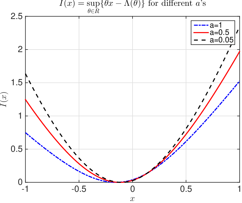
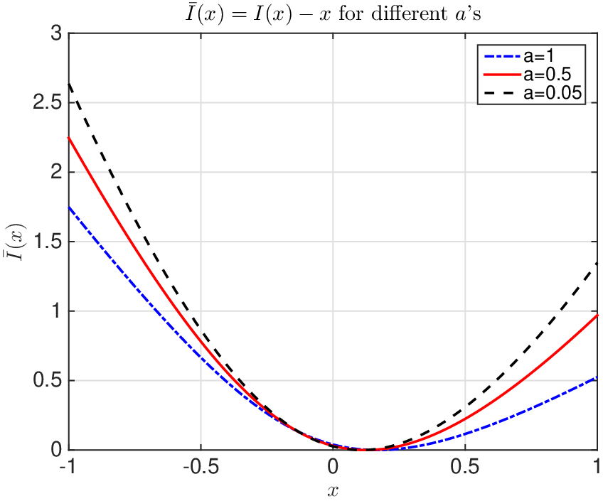
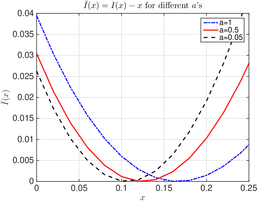
Figure 3 shows the rate function for selected aa values. One should notice as aa increases, the growth rate of I⁡(x)I(x) increases. This is expected as more rare events occur when aa increases, so the rate function I⁡(x)I(x) tends to be smaller. The right figure is the zoom-in of the left figure and it shows the minimums do not coincide. Rate function I¯​(x)\bar{I}(x) is shown in Figure 4 and it has similar behaviors as I⁡(x)I(x) in Figure 3. Figure 5 shows the asymptotic of implied volatility in the large-maturity and large-strike regime for different aa values. The affine point jump-diffusion model can capture the implied volatility smiles in this regime. Forde and Jacquier, 2011 found similar implied volatility smiles for the Heston model in the same regime. Consider the At-The-Money cases when x=0x=0, the ATM volatility increases as aa increases. It is because as more rare events occur, the implied volatility is higher. Besides, the growth rate of the implied volatility into In-The-Money/Out-The-Money increases as aa increases.

Numerical results for different β\beta values are shown in Figures 6, 7 and 8. Because the parameter β\beta controls the strength of the self-exciting process intensity, so varying β\beta has similar effects as varying aa.

Refer to caption
Refer to caption
Figure 3: Left: I⁡(x)I(x) for a=0.05,0.5a=0.05,~0.5 and 11; Right: Zoom-in of left figure near I⁡(x)=0I(x)=0.
Refer to caption
Refer to caption
Figure 4: Left: I¯​(x)\bar{I}(x) for a=0.05,0.5a=0.05,~0.5 and 11; Right: Zoom-in of left figure near I¯​(x)=0\bar{I}(x)=0.
Refer to caption
Figure 5: σ∞2​(x)\sigma_{\infty}^{2}(x) for a=0.05,0.5a=0.05,~0.5 and 11.
Refer to caption
Refer to caption
Figure 6: Left: I⁡(x)I(x) for β=0.1,0.25\beta=0.1,~0.25 and 0.50.5; Right: Zoom-in of left figure near I⁡(x)=0I(x)=0.
Refer to caption
Refer to caption
Figure 7: Left: I¯​(x)\bar{I}(x) for β=0.1,0.25\beta=0.1,~0.25 and 0.50.5; Right: Zoom-in of left figure near I¯​(x)=0\bar{I}(x)=0.
Refer to caption
Figure 8: σ∞2​(x)\sigma_{\infty}^{2}(x) for β=0.1,0.25\beta=0.1,~0.25 and 0.50.5.

Numerical examples in fixed-maturity large, small-strike and large-strike are presented. The left figure in Figure 9 shows the ratio of Black-Scholes implied volatility to log-moneyness in the fixed-maturity and large-strike regime for different aa values; while right figure displays the ratio in the fixed-maturity and small-strike regime. The maturity TT is chosen within a reasonable range. In both figures, we observe that, for a given TT, the ratio of implied volatility to log-moneyness increases as the self-exciting intensity parameter aa increases. It is interesting to point out that, in these regimes, the ratio of Black-Scholes implied volatility to log-moneyness decreases as maturity increases. This is practically observed on an implied volatility surface. Results for various values of β\beta’s are provided in Figure 10. We obtain similar results because β\beta controls the strength of the self-exciting process as well.

Refer to caption
Refer to caption
Figure 9: Left: lim supk→+∞σBS2​(k,T)|k|\mathop{\limsup}\limits_{k\rightarrow+\infty}\frac{\sigma^{2}_{\text{BS}}(k,T)}{|k|} (fixed-maturity large-strike) for a=0.05,0.5a=0.05,~0.5 and 11; Right: lim supk→−∞σBS2​(k,T)|k|\mathop{\limsup}\limits_{k\rightarrow-\infty}\frac{\sigma^{2}_{\text{BS}}(k,T)}{|k|} (fixed-maturity small-strike) for a=0.05,0.5a=0.05,~0.5 and 11.
Refer to caption
Refer to caption
Figure 10: Left: lim supk→+∞σBS2​(k,T)|k|\mathop{\limsup}\limits_{k\rightarrow+\infty}\frac{\sigma^{2}_{\text{BS}}(k,T)}{|k|} (fixed-maturity large-strike) for β=0.1,0.25\beta=0.1,~0.25 and 0.50.5; Right: lim supk→−∞σBS2​(k,T)|k|\mathop{\limsup}\limits_{k\rightarrow-\infty}\frac{\sigma^{2}_{\text{BS}}(k,T)}{|k|} (fixed-maturity small-strike) for β=0.1,0.25\beta=0.1,~0.25 and 0.50.5.

4 Concluding Remarks

  In this paper, we study the asymptotic behaviors of the implied volatility of an affine jump-diffusion model. Let Xt=log⁡(St/S0)X_{t}=\log(S_{t}/S_{0}) and StS_{t} follows an affine jump-diffusion model under risk-neutral measure. By applying the Feynman-Kac formula, we compute the moment generating function for XtX_{t}. An explicit form of the moment generating function can be found by solving a set of ordinary differential equations. A large-maturity large deviation principle for XtX_{t} is obtained by using the Gärtner-Ellis Theorem. We characterize the asymptotic behaviors of implied volatility for XtX_{t} in the joint regime of large-maturity and large-strike regime. We use Lee’s moment formula to derive the asymptotics for Black-Scholes implied volatility in the fixed-maturity, large-strike and fixed-maturity, small-strike regimes. Numerical studies are provided to validate the theoretical work. We observe the volatility smiles in the joint regime of large-maturity and large-strike. As the self-exciting intensity parameter (aa or β\beta) increases, which means more rare events tending to occur, the ATM volatility increases and volatility smile tends to be more convex. Ratios of Black-Scholes implied volatility to log-moneyness in fixed-maturity large, small-strike and large-strike regimes are shown. For a given maturity TT, as the self-exciting parameter (aa or β\beta) increases, the ratio of implied volatility to log-moneyness increases. In these two regimes, we observe the ratio of implied volatility to log-moneyness declines as the maturity increases and this is usually detected on an implied volatility surface in practice.

Acknowledgments

Nian Yao was supported in part by Natural Science Foundation of Guangdong Province under Grant 2019A1515012192. Author Nian Yao and Zhiqiu Li acknowledge Dr. Lingjiong Zhu for many useful discussions and comments.

References

  • Aït-Sahalia et al., (2015) Aït-Sahalia, Y., Cacho-Diaz, J., and Laeven, R. J. (2015). Modeling financial contagion using mutually exciting jump processes. Journal of Financial Economics, 117(3):585–606.
  • Alfonsi et al., (2019) Alfonsi, A., Krief, D., and Tankov, P. (2019). Long-time large deviations for the multiasset wishart stochastic volatility model and option pricing. SIAM Journal on Financial Mathematics, 10(4):942–976.
  • Bacry et al., (2015) Bacry, E., Mastromatteo, I., and Muzy, J.-F. (2015). Hawkes processes in finance. Market Microstructure and Liquidity, 1(01):1550005.
  • Crane and Sornette, (2008) Crane, R. and Sornette, D. (2008). Robust dynamic classes revealed by measuring the response function of a social system. Proceedings of the National Academy of Sciences, 105(41):15649–15653.
  • Dembo and Zeitouni, (1998) Dembo, A. and Zeitouni, O. (1998). Large Deviations Techniques and Applications. Second ed. Springer, New York.
  • Duffie et al., (2000) Duffie, D., Pan, J., and Singleton, K. (2000). Transform analysis and asset pricing for affine jump-diffusions. Econometrica, 68(6):1343–1376.
  • Errais et al., (2010) Errais, E., Giesecke, K., and Goldberg, L. R. (2010). Affine point processes and portfolio credit risk. SIAM Journal on Financial Mathematics, 1(1):642–665.
  • Forde and Jacquier, (2011) Forde, M. and Jacquier, A. (2011). The large-maturity smile for the heston model. Finance Stoch., 15:755–780.
  • Forde and Pogudin, (2013) Forde, M. and Pogudin, A. (2013). The large-maturity smile for the sabr and cev-heston models. International Journal of Theoretical and Applied Finance, 16(08):1350047.
  • Gao and Zhu, (2019) Gao, X. and Zhu, L. (2019). Affine point processes: Refinements to large-time asymptotics. arXiv preprint arXiv:1903.06371.
  • (11) Hawkes, A. G. (1971a). Point spectra of some mutually exciting point processes. Journal of the Royal Statistical Society: Series B (Methodological), 33(3):438–443.
  • (12) Hawkes, A. G. (1971b). Spectra of some self-exciting and mutually exciting point processes. Biometrika, 58(1):83–90.
  • Jacquier et al., (2013) Jacquier, A., Keller-Ressel, M., and Mijatović, A. (2013). Large deviations and stochastic volatility with jumps: asymptotic implied volatility for affine models. Stochastics An International Journal of Probability and Stochastic Processes, 85(2):321–345.
  • Jacquier and Roome, (2016) Jacquier, A. and Roome, P. (2016). Large-maturity regimes of the heston forward smile. Stochastic Processes and their Applications, 126(4):1087–1123.
  • Kou, (2002) Kou, S. G. (2002). A jump-diffusion model for option pricing. Management science, 48(8):1086–1101.
  • Lee, (2004) Lee, R. W. (2004). The moment formula for implied volatility at extreme strikes. Mathematical Finance, 14(3):469–480.
  • Ma et al., (2017) Ma, Y., Shrestha, K., and Xu, W. (2017). Pricing vulnerable options with jump clustering. Journal of Futures Markets, 37(12):1155–1178.
  • Merton, (1976) Merton, R. C. (1976). Option pricing when underlying stock returns are discontinuous. Journal of financial economics, 3(1-2):125–144.
  • Mohler et al., (2011) Mohler, G. O., Short, M. B., Brantingham, P. J., Schoenberg, F. P., and Tita, G. E. (2011). Self-exciting point process modeling of crime. Journal of the American Statistical Association, 106(493):100–108.
  • Ogata, (1988) Ogata, Y. (1988). Statistical models for earthquake occurrences and residual analysis for point processes. Journal of the American Statistical association, 83(401):9–27.
  • Reynaud-Bouret et al., (2010) Reynaud-Bouret, P., Schbath, S., et al. (2010). Adaptive estimation for hawkes processes; application to genome analysis. The Annals of Statistics, 38(5):2781–2822.
  • Zhang et al., (2015) Zhang, X., Blanchet, J., Giesecke, K., and Glynn, P. W. (2015). Affine point processes: Approximation and efficient simulation. Mathematics of Operations Research, 40(4):797–819.
  • Zhang and Glynn, (2018) Zhang, X. and Glynn, P. W. (2018). Affine jump-diffusions: Stochastic stability and limit theorems. arXiv preprint arXiv:1811.00122.
  • Zhu, (2014) Zhu, L. (2014). Limit theorems for a cox-ingersoll-ross process with hawkes jumps. Journal of Applied Probability, 51(3):699–712.