Online Binary Space Partitioning Forests
Xuhui Fan Bin Li Scott A. Sisson
School of Mathematics and Statistics University of New South Wales xuhui.fan@unsw.edu.au School of Computer Science Fudan University libin@fudan.edu.cn School of Mathematics and Statistics University of New South Wales scott.sisson@unsw.edu.au
Abstract
The Binary Space Partitioning-Tree (BSP-Tree) process was recently proposed as an efficient strategy for space partitioning tasks. Because it uses more than one dimension to partition the space, the BSP-Tree Process is more efficient and flexible than conventional axis-aligned cutting strategies. However, due to its batch learning setting, it is not well suited to large-scale classification and regression problems. In this paper, we develop an online BSP-Forest framework to address this limitation. With the arrival of new data, the resulting online algorithm can simultaneously expand the space coverage and refine the partition structure, with guaranteed universal consistency for both classification and regression problems. The effectiveness and competitive performance of the online BSP-Forest is verified via simulations on real-world datasets.
1 Introduction
The BSP-Tree Process [Fan et al., 2016a, Fan et al., 2018a, Fan et al., 2019b] is a stochastic space partitioning process defined in a multi-dimensional space with a binary-partition strategy. Its general goal is to identify meaningful “blocks” in the space, so that data within each block exhibits some form of homogeneity. Similar to other space partitioning processes [Kemp et al., 2006, Roy and Teh, 2009, Nakano et al., 2014, Fan et al., 2018b], the BSP-Tree Process can be applied in many areas, including relational modeling [Kemp et al., 2006, Airoldi et al., 2009, Fan et al., 2016b, Fan et al., 2019a], community detection [Nowicki and Snijders, 2001, Karrer and Newman, 2011], collaborative filtering [Porteous et al., 2008, Li et al., 2009], and random forests [Lakshminarayanan et al., 2014].
Instead of the axis-aligned cuts adopted in most conventional approaches [Kemp et al., 2006, Roy and Teh, 2009, Nakano et al., 2014], the BSP-Tree Process implements oblique cuts (in more than one dimension) to recursively partition the space into new sub-spaces. In this way, it can describe the dimensional dependence more efficiently, in terms of fewer cuts or improved prediction performance. In addition, the BSP-Tree Process has the attractive theoretical property of self-consistency. Based on this property, a projective system [Crane, 2012] can be constructed to ensure distributional invariance, when restricting the process from a larger domain to a smaller one, and safely extend a finite domain to multi-dimensional infinite space.
Despite the existing clear potentials, there are two main challenges in the BSP-Tree Process. (1) Scalability: Its batch learning mode is unappealing given the practical real, large-scale datasets, as multiple scans over the data are required. (2) Theoretical properties: Moving from a batch to an online learning algorithm, rigorous universal consistency properties are required to ensure the theoretical correctness of the underlying BSP-Tree Process prior as the domain varies with the arrival of new data. This can be challenging due to the recursive structure of the partition strategy and the Markov property of partition refinement.
In this paper we propose an online BSP-Forest framework to address these challenges. Instead of batch model training, our framework sequentially incorporates each data point and updates the model without the need for data labels. The tree structure update in the forest is implemented in two stages. (i) Node coverage expansion: Within the nodes (all of nodes are convex polyhedron-shaped) of each tree, we focus on the convex hull that contains all of its allocated datapoints. When a new point arrives in this node but falls outside the convex hull, we enlarge the hull and change the tree structure. (ii) Refinement over existing partitions: We use a monotonically increasing budget sequence for new node creation, meaning that more data tend to result in finer partitions. These stages are each supported by the self-consistency and Markov properties of the BSP-Tree Process. In addition, we demonstrate its universal consistency by proving that the online BSP-Forest will converge to the Bayesian error for all possible label distributions. The effectiveness and competitive performance of the online BSP-Forest in classification and regression is verified through extensive simulation studies.

2 The BSP-Tree Process
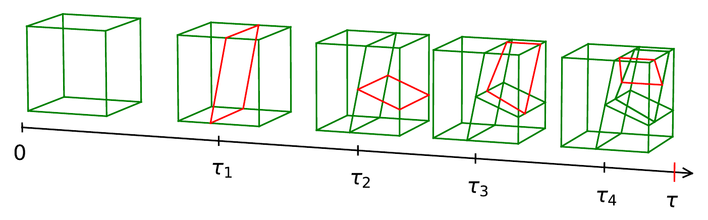
The BSP-Tree Process [Fan et al., 2018a, Fan et al., 2019b] is a time-indexed, right-continuous Markov jump process. At any point of the time line, the BSP-Tree Process takes the state of a hierarchical binary partition over the multi-dimensional space (Figure 1). Starting at time with the initial space (no cuts), new random oblique cuts are created over time. Each selected region for partition is named a block, where each cut recursively divides the block into two smaller ones. Given any two time points , the partition at is a further refinement of the partition at (e.g. there might be additional cuts).
The distinguishing feature of the BSP-Tree Process is the oblique cut it uses to partition the space. Unlike its axis-aligned cut counterparts [Roy and Teh, 2009], the BSP-Tree Process uses more than one dimension to form the cutting hyperplanes, and so is a more efficient cutting strategy (i.e. it uses fewer cuts to achieve similar performance).
We introduce some notation before formally describing the BSP-Tree Process. For a -dimensional space (which is assumed to be a convex polyhedron), we let denote the set of all two dimensional pairs. For each element in , denotes the projection of onto the dimensions of (which becomes a 2-dimensional polygon), denotes the corresponding perimeter, lies in the 2D space of dimensions and represents the line segment of in the direction of the angle (in the dimensions of ; Figure 1 (Right)), is the cutting position in the segment , represents the cost of a cut in the time line and represents one cutting hyperplane with all these variables.
Algorithm 1 describes generation of the recursive hierarchical partition under the BSP-Tree Process. Algorithm 2 generates an oblique cut in a particular block ; the right part of Figure 1 illustrates Lines 3–6 in Algorithm 2. To generate an oblique cut in , we first generate the cost of the proposed cut from an Exponential distribution, parameterised by the sum of perimeters of all of the block’s two-dimensional projections (Line ). If so the cost of the candidate cut exceeds the budget , the cut is not generated and the current block is returned as the final partition structure in that branch (Line ); otherwise we sample a 2-dimensional pair in proportion to (Line ). The cutting hyperplane will be generated in this dimensional pair, and is parallel to the other dimensions. Line generates the angle with density proportional to , and the cutting position uniformly in the segment for the pair . The cutting hyperplane is then formed as and cuts the block into two new sub-blocks (Line ). Line recursively generates independent BSP partitions on the new blocks .
One attractive property of BSP-Tree Process is that it is self-consistent [Fan et al., 2018a, Fan et al., 2019b]. This helps to provide an efficient convex hull representation of nodes in a tree when in a multi-dimensional space.
Theorem 1.
(Self-Consistency) Given a partition sampled from the BSP-Tree Process on the convex domain , let be a convex subdomain of . Then, the restriction of this partition on has the same distribution as the restriction directly sampled from the BSP-Tree Process on .
3 Online BSP-Forests
We have an observed set of labelled datapoints which arrive over time, where is a -dimensional feature vector and is the corresponding label. We have an additional set of feature data for predictive testing. The goal is to predict the unknown labels of the testing data, based on their feature data and the observed training data .
Similar to the standard random forest [Breiman, 2000, Biau et al., 2008], which assumes the partition is generated independently of the data labels, the online BSP-Forest does not use the data labels, but considers the partition structure within the convex hulls spanned by the arrival feature data . Each node in the BSP-Tree records two items: the convex hull that covers its constituent datapoints, and the possible hyperplane cutting this hull. A nested set may be used to represent the tree structure of these nodes. , is defined as , where refers to the given convex hull, is ’s cutting hyperplane, and () represents the left (right) child node of . Since is generated depending on the feature points , it can be generated as , where is an increasing budget sequence.
Further, the BSP-Forest, an ensemble of independent BSP-Trees sampled over the feature space, may be used for regression/classification tasks. In this way, the predictive label distribution on any feature data is , where is the predictive distribution of under the -th BSP-Tree. That is, the predictive distribution is a finite sample approximation to , which becomes more accurate for a larger .

Algorithm 3 (oBSP, along with Algorithms 4 and 6) specifies the strategy of building the online BSP-Forest in detail. Starting from a set of empty nodes, the online BSP-Forest updates each BSP-Tree once new training data arrives. From the BSP-Tree constructed from the previous datapoints, this procedure then defines a conditional BSP-Tree Process (cBSP) such that, following the distributional invariance self-consistency property between the domain and its subdomain, and the Markov property in the time line, the new partition based on up to datapoints is constructed as
It then follows that the new partition has the same distribution as
That is, the distribution of an online BSP-Tree trained (using the cBSP) on sequentially arriving data, is the same as that of a BSP-Tree () directly trained on the full dataset. Different shuffling arrangement on the datapoints would not affect the partition result.
Conditional BSP-Tree Process (cBSP):
Algorithm 4 describes the procedural detail of the cBSP when incorporating a new datapoint . Based on the location of and the (possibly) generated cut cost, each BSP-Tree might update the tree structure, enlarge the hull coverage, or implement a new cut in the tree nodes. Figure 2 illustrates each of these cases:
- (i)
Points form a -level BSP-Tree (Lines 1–6, Algorithm 4), where are in the right level- convex hull and is in the left one.
- (ii)
A new point arrives outside the level- convex hull. A new cost value is generated (Line 7, Algorithm 4). This new cost is compared with the cost associated with the cut-line in the level- convex hull. If (Line 8, Algorithm 4), a cut-line not crossing into the level- convex hull is generated (see Section 1 of the supplementary material), and a new level- convex hull is formed from the previous level- hull and the point . All previously existing level- convex hulls in this branch are demoted to level-() as a consequence of creating the new right level- convex hull.
- (iii)
A new point arrives outside the level- convex hull and the new generated cost value is larger than the current cost value . The cut-line (red solid line) allocates the new point to the rightmost level- convex hull. Since this is a leaf node (no cut-lines inside), it forms a new level- convex hull including the new point (Lines 13 and 15, Algorithm 4).
- (iv)
A new point arrives inside the level- convex hull. Different levels of cutting lines are repeatedly compared to until is compared with a leaf node (Line 15, Algorithm 4). Since a larger budget (i.e. the budget for datapoints) is provided, new cuts may still be generated within the leaf node.
It is noted that Lines in Algorithm 4 restrict a block to be cut only if it contains more than datapoints. If we have set an overly-large budget sequence, which prefers to generate small and trivial blocks, this restriction can help the algorithm avoid the overfitting issue.
Benefits of a convex hull representation:
Cutting the full -dimensional polyhedron generated from a series of cutting hyperplanes on the original domain is a challenging task. This is because completely indexing of this polyhedron requires extensive geometric manipulation, including calculating the intersection of multiple hyperplanes, determining if two hyperplanes intersect in the presence of other hyperplanes, and listing all vertices of the polyhedron.
Instead, implementing the hyperplane cut on the convex hull greatly simplifies these issues. The projection of the convex hull on any two dimensions can be simply obtained by extracting the elements of in these dimensions, and then using a conventional convex hull detection algorithm (such as the Graham Scan algorithm [Graham, 1972] with a computational complexity of ). Algorithm 6 describes the way of generating the hyperplane cut in a convex hull.
The self-consistency property (Theorem 1) of the BSP-Tree Process enables us conveniently and immediately have that:
Corollary 1.
The hyperplane restricted to the convex hull has the same distribution as if it was first generated on the “full” polyhedron, and then restricted to the convex hull.
That is, the partitions of the BSP-Tree Process on the full space and on the data spanned convex hull will produce identical inferential outcomes.
Computational complexity:
In the optimal case and assuming the BSP-Tree formed by the streaming data is a balanced tree (which keeps the height of trees in a complexity of ), the computational complexity of a single BSP-Tree is . When it is of the same magnitude as the of the Mondrian Forest [Lakshminarayanan et al., 2014, Lakshminarayanan et al., 2016] (also in the optimal case) in terms of , the additional scaling factor is the price of more efficient cuts. In this perspective, this online BSP-Forest might be more suitable for low-dimensional regression/classification problems. In practice, we may alleviate this additional computational cost by using less hierarchical structure (through settings of smaller budget , see experiments in Section 5.3). The convex hull calculation is , which does not influence the general computational complexity.
In the worst case, when the height of the BSP-Tree equals to the number of datapoints () and each level has one split only, the computational complexity of the online BSP-Forest turns into (which is the same as the Mondrian Forest in terms of ). This complexity is still smaller than that of the batch version of a Random Forest ( [Lakshminarayanan et al., 2014, Lakshminarayanan et al., 2016]) in terms of . It is also noted that the online BSP-Forest can be easily made to run in parallel as its component trees are updated in an independent manner.
When a new sample arrives, the computational complexity depends on the existing tree structure: if the BSP-tree is a balanced tree, the complexity is ; if the height of the BSP-tree equals to the number of existing samples (i.e., the worst case), the complexity is .
In the memory usage part, the online BSP-Forest requires the same amount of as the Mondrian Forest. That is to say, each leaf node of the BSP-Tree would store all its belonging datapoints for future splitting.
Empirical label distribution:
For the label distribution , we use the empirical distribution of the labels from the training data to represent the label distribution on each of the leaf nodes. For classification tasks, we use a majority vote over the label predictions of each tree in the online BSP-Forest; for regression tasks, we use the mean value of the trees’ label predictions at the given point. According to [Breiman, 2000, Biau et al., 2008, Mourtada et al., 2017], this simple empirical approach usually performs competitively compared to constructing complex Bayesian models on the label distribution.
Universal consistency:
As a larger value of the budget indicates a deeper tree structure and more complex partitions, the increasing budget sequence indicates that the online BSP-Forest will produce more refined partitions with increasing amounts of data. This is consistent with the intuition behind, and a central tenet of, Bayesian nonparametrics. Similar observations (for Mondrian Forest only) has also been obtained in [Mourtada et al., 2017]. Further, it shows that such an increasing budget sequence is the key to guarantee the algorithm’s performance converge to the optimal for all distributions over the labels and features.
More formally, let denote the error probability of these tree-structured online algorithm . Using to denote the Bayesian error rate, which is generated by the optimal classifier. As the increasing budget with results in finer partitions (i.e. more blocks and “smaller” block sizes), these online algorithms ensure there are a sufficiently large number of datapoints in each block, and its performance approaches the Bayesian error.
In order to discuss this “universal consistency” in the online BSP-Forest setting, we first investigate particular properties of an oblique line slice of the BSP-Tree Process.
Lemma 1.
(Oblique line slice) For any oblique line that crosses into the domain of a BSP-Tree Process with budget , its intersection points with the partition forms a homogeneous Poisson Process with intensity .
Lemma 2 can enable us to describe basic characteristics (e.g. size, number) of the blocks of the BSP-Tree. Based on Lemma 2, the theoretical work of [Mourtada et al., 2017] and Theorem 6.1 of [Devroye et al., 2013] and set restrictions on the budget sequence, we can obtain the resulting universal consistency for the online BSP-Forest as:
Theorem 2.
If and , then for classification tasks, we have .
This universal consistency can be applied on any format of dataset as the result does not restrict the distribution of or the prediction function .
Using the same proof techniques of [Mourtada et al., 2017], we can obtain minimax convergence rate for the regression trees task as (the result for the classification trees can be obtained in a similar way):
Theorem 3.
Suppose that the label is generated by a Lipschitz function on the cubic space . Let be an online BSP-Forest algorithm and that the budget sequence satisfies . Then, the following upper bound holds:
| (1) |
for sufficiently large , which corresponds to the minimax rate over the set of Lipschitz functions.
This result can be used for the guide of appropriately choosing the values on the budget sequence.
4 Related Work
Since its introduction in the early 2000s, the random forest [Breiman, 2001, Breiman, 2000] has become a state-of-the-art method for typical classification and regression tasks. The literature is too vast to provide a comprehensive but compact survey, and so we focus on its online versions. For the frequentist-styled online random forest algorithms, they were developed by [Denil et al., 2013, Saffari et al., 2009, Domingos and Hulten, 2000]. The first two algorithms start from empty trees, and then grow the tree with more data based on evaluating a score function for each potential split position. As this score function relates to training performance, the node splitting procedure is label dependent. However, memory usage is inefficient in these two algorithms as the scores must be computed and stored for each potential split position. The third algorithm proposes to build online decision trees using constant memory and constant time per datapoint. These partitions are inefficient as only one feature is involved in the split procedure.
The Purely Random Forest (PRF) algorithm [Genuer, 2012, Arlot and Genuer, 2014] assumes tree generation is independent of data labels. When the split position is random, which is similar to the Mondrian Forest and the online BSP-Forest, the corresponding distribution on the resulting partition is not self-consistent. Further, its batch learning framework is not amenable to large-scale learning. [Genuer, 2012] proves that the PRF can achieve the minimax rate for estimating Lipschitz functions in the -dimensional case for single trees. [Arlot and Genuer, 2014] extends the analysis to forest settings and shows an improved convergence rate for smooth regression functions.
The Mondrian Forest [Lakshminarayanan et al., 2014, Lakshminarayanan et al., 2016] is the closest related method to the online BSP-Forest, as it uses the Mondrian process [Roy et al., 2007, Roy and Teh, 2009, Roy, 2011] to place a probability distribution over all the d-tree-based partitions of the domain. In regularising the Mondrian-Forest to be consistent, [Mourtada et al., 2017] sets the budget parameter to increase with the amount of data, and it then achieves the minimax rate in multi-dimensional space for single decision trees. [Mourtada et al., 2018] displays the advantage of Forest settings by showing improved convergence results.

In its favour, and in contrast to the above methods, the online BSP-Forest uses more than one dimension to implement node splits, and is accordingly more efficient. Further, the arrival of new data is dealt with by considering both the expansion of the feature space (i.e. the convex hull representation of tree nodes) and expansion of the budget line (i.e. an increasing budget sequence). This ensures the online BSP-Forest is represented efficiently and theoretically guaranteeing universal consistency.
5 Experiments
We examine the performance of the online BSP-Forest in regression and classification tasks. Unless specified, in each analysis, we re-scale the data features to the domain space, set the parameter of the Exponential distribution of cut cost to (half of the perimeter of the (-dimensional) block ), and specify the budget sequence as . Through these experiments, we show that (1) the online-BSPF performs better than other online algorithms and at the same time, it keeps competitive to the batch trained algorithms in regression and classification tasks; (2) the online-BSPF produce more efficient partitions than the Mondrian Forest algorithm.

The online BSP-Forest is compared with several state-of-the-art methods: (1) a random forest (RF) [Breiman, 2001]; (2) Extremely Randomized Trees (ERT) [Geurts et al., 2006]; (3) a Mondrian Forest (MF) with fixed budget [Lakshminarayanan et al., 2014, Lakshminarayanan et al., 2016]; and (4) a Mondrian Forest with increasing budget [Mourtada et al., 2017]. The number of trees is fixed to to avoid high computational costs. For the RF and ERT, we use the implementations in the scikit-learn toolbox [Pedregosa et al., 2011]. For the MF with infinite budget, we use the scikit-garden implementation. For the parameter tuning in the RF and ERT, we use the GridSearchCV package in the scikit-learn toolbox and focus on tuning the features of “maxfeatures”, which concerns the number of features considered when selecting the best split. Each test case was replicated times, and we report summary means and standard errors for each measure.
| Dataset | RF | ERT | MF (fixed ) | MF (increasing ) | online BSP-Forest |
|---|---|---|---|---|---|
| Apartment | |||||
| Airline () | |||||
| Airline () | |||||
| Airline () |

5.1 Classification
We examine the classification accuracy of the online BSP-Forest through four real datasets [Chang and Lin, 2011] used in [Lakshminarayanan et al., 2016, Denil et al., 2013]: satimages (), letter (), dna () and usps (). For all these datasets, we use Principle Component Analysis (PCA) to extract principle components before deploying the models. As we have mentioned that the online BSP-Forest is suitable for low dimensional case, this dimensional reduction technique helps us to largely reudce the computational cost (e.g. DNA dataset with features). For each dataset, we use different ratios of the whole data as the training data and use the rest as the testing data. For the label prediction, we would first use the majority vote to determine the class label of the nodes in each tree and then again use the majority vote over the datapoints’ covered nodes to predict the label for the data point.
The detail classification performance (under different ratios of training data) for each dataset is displayed in Figure 3. Except for the dna dataset, the performance of the online-BSPF is quite competitive to RF and ERT and much better than the Mondrian Forest algorithm in other three datasets. As RF, ERT and MF proceed each cut using one feature only, the effectiveness of oblique cuts can be verified even for the online setting.
5.2 Regression
Friedman’s Function (simulated data):
The performance of the online BSP-Forest is first evaluated on the Friedman’s function [Friedman, 1991, Chipman et al., 2010, Linero and Yang, 2017]. In this setting, each datapoint is generated from a -dimensional uniform distribution, and its label takes the form:
| (2) |
, where . Friedman’s function consists of two nonlinear terms, two linear terms and an interaction term.
We compute the RMSE (root mean squared error) under each method as the true function is known, for different numbers of datapoints , and for two different dimensional setups: where all dimensions are informative, and where only the first 5 dimensions are informative. The results are shown in Figure 8. The online BSP-Forest performs better (in RMSE) than the two (online) Mondrian-Forests, with improvement in RMSE.
Since the three online algorithms are implemented independently of the data labels, it is not surprising that they perform worse than the batch trained RF and ERT. The performance differential is greater when noisy dimensions () are added. Because the online-BSPF purely uses the generative process to generate the tree structure, it distinguishes between meaningful and noisy dimensions less well. Similar observations have been reported in [Lakshminarayanan et al., 2016]. We may overcome such a performance deficit by increasing the budget, which will permit additional cuts in meaningful dimensions in spite of some less useful cuts in noisy dimensions.
UK Apartment Price data:
The performance of the online BSP-Forest is examined on the UK Apartment Price Data [Hensman et al., 2013], which records the selling price of apartments in the UK from February to October 2012. We take the apartment price as the target label data, and use GPS coordinates (coarsely estimated based on the apartment’s postcode and GPS database) as the feature data ().
To evaluate the performance of the online BSP-Forest, we randomly sample of the data as the training data and predict the price values on the remaining data. Row in Table 1 displays the RMSE values of each method. While, as before, the RF and ERT methods perform better than the three online learning algorithms, their RMSE values are similar. Also, the online BSP-Forest outperforms the more directly comparable Mondrian Forest variants.
Airline Delay data:
We finally analyse the regression performance of the online BSP-Forest on the airline delay data [Hensman et al., 2013]. We wish to predict flight delay time () based on factors (). Following [Deisenroth and Ng, 2015, Lakshminarayanan et al., 2016], , these factors are set to include the age of the plane, prospective flight distance, prosepctive flight airtime, departure time, arrival time, day of the week, day of the month and month of the year.
Following the settings of [Deisenroth and Ng, 2015, Lakshminarayanan et al., 2016], we set the number of training datapoints as , and million, and specify the test data as the observations immediately following the training data. Rows 2–4 in Table 1 display each methods’ RMSE values. Similar conclusions can be drawn as for the previous analyses: while the RF and ERT perform better than any the online algorithm, the online BSP-Forest is the best performing online algorithm. In the exceptional case of , where the MF with increasing budget performs better than the online BSP-Forest, the former variance () is larger than the later ().
5.3 Efficiency of the cutting strategy
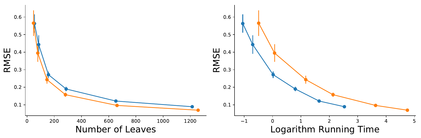
Cutting efficiency is a primary advantage of the online BSP-Forest. We quantitatively explore this efficiency issue through the simple function: . Two different cases are investigated: (1) different budget sequences. We set and the budget sequence as ; (2) different number of datapoints. Based on the results of case (1), we set and let the number of datapoints as for case (2). Performance results are shown in Figure 5.
For case (1), the left two sub-figures confirm that, for different budget sequences, the online BSP-Forest can always obtain better RMSE performance than the Mondrian Forest. The numbers of leaves are also similar between these two algorithms. It is noted that, as each node is restricted to be cut only if it contains more than datapoints, these algorithms’ performance becomes stable even for large value settings of budget sequences. For case (2), the right two sub-figures indicate the consistent better performance of the online-BSPF for different number of datapoints, with the price of requiring a bit longer running time (due to the computational cost of ).
6 Conclusion & Future work
In this paper we have developed an online BSP-Forest framework that addresses the scalability and theoretical challenges of the online BSP-Forest algorithm. Through a non-trivial scheme for efficiently incorporating sequential datapoints, the model construction for the online BSP-Forest follows the same distribution as that for the batch setting. By using more than one dimension to cut the underlying space, the online BSP-Forest is a demonstrably efficient model for classification and regression tasks. Our experimental results (Section 5) verify that the online BSP-Forest consistently outperforms the Mondrian-Forest, and is competitive with other batch random forest models.
For the future work, the Random Tesselation Forest [Ge et al., 2019] has extended the BSP-Tree Process by generating arbitrary sloped cutting hyperplanes in -dimensional spaces. Extending the Random Tesselation Forest to the online learning setting and comparing with the online BSP-Forest would be interesting work. Recently, [O’Reilly and Tran, 2020] uses the technique of iteration stable (STIT) tessellations to efficiently generate arbitrary sloped cuts. It might be possible to use their method to further reduce the factor to the computational cost of the online BSP-Forest and make the online BSP-Forest suitable for high-dimensional data as well.
Acknowledgements
Xuhui Fan and Scott A. Sisson are supported by the Australian Research Council through the Australian Centre of Excellence in Mathematical and Statistical Frontiers (ACEMS, CE140100049), and Scott A. Sisson through the Discovery Project Scheme (DP160102544). Bin Li is supported by Shanghai Municipal Science & Technology Commission (16JC1420401) and the Program for Professor of Special Appointment (Eastern Scholar) at Shanghai Institutions of Higher Learning.
References
- [Airoldi et al., 2009] Airoldi, E., Blei, D., Fienberg, S., and Xing, E. (2009). Mixed membership stochastic blockmodels. In NIPS, pages 33–40.
- [Arlot and Genuer, 2014] Arlot, S. and Genuer, R. (2014). Analysis of purely random forests bias. arXiv preprint arXiv:1407.3939.
- [Balog and Teh, 2015] Balog, M. and Teh, Y. W. (2015). The mondrian process for machine learning. arXiv preprint arXiv:1507.05181.
- [Biau et al., 2008] Biau, G., Devroye, L., and Lugosi, G. (2008). Consistency of random forests and other averaging classifiers. Journal of Machine Learning Research, 9(Sep):2015–2033.
- [Breiman, 2000] Breiman, L. (2000). Some infinity theory for predictor ensembles. Technical report, Technical Report 579, Statistics Dept. UCB.
- [Breiman, 2001] Breiman, L. (2001). Random forests. Machine Learning, 45(1):5–32.
- [Chang and Lin, 2011] Chang, C.-C. and Lin, C.-J. (2011). Libsvm: A library for support vector machines. ACM Trans. Intell. Syst. Technol., 2(3):27:1–27:27.
- [Chipman et al., 2010] Chipman, H. A., George, E. I., and McCulloch, R. E. (2010). Bart: Bayesian additive regression trees. The Annals of Applied Statistics, 4(1):266–298.
- [Crane, 2012] Crane, H. (2012). Infinitely Exchangeable Partition, Tree and Graph-valued Stochastic Processes. PhD thesis.
- [Deisenroth and Ng, 2015] Deisenroth, M. P. and Ng, J. W. (2015). Distributed Gaussian processes. In ICML, pages 1481–1490.
- [Denil et al., 2013] Denil, M., Matheson, D., and Freitas, N. (2013). Consistency of online random forests. In ICML, volume 28, pages 1256–1264.
- [Devroye et al., 2013] Devroye, L., Györfi, L., and Lugosi, G. (2013). A probabilistic theory of pattern recognition, volume 31. Springer Science & Business Media.
- [Domingos and Hulten, 2000] Domingos, P. and Hulten, G. (2000). Mining high-speed data streams. In Kdd, volume 2, page 4.
- [Fan et al., 2019a] Fan, X., Li, B., Sisson, S., Li, C., and Chen, L. (2019a). Scalable deep generative relational model with high-order node dependence. In NeurIPS, pages 12637–12647.
- [Fan et al., 2018a] Fan, X., Li, B., and Sisson, S. A. (2018a). The binary space partitioning-tree process. In AISTATS, volume 84 of Proceedings of Machine Learning Research, pages 1859–1867.
- [Fan et al., 2018b] Fan, X., Li, B., and Sisson, S. A. (2018b). Rectangular bounding process. In NeurIPS, pages 7631–7641.
- [Fan et al., 2019b] Fan, X., Li, B., and Sisson, S. A. (2019b). Binary space partitioning forests. In AISTATS, volume 89, pages 3022–3031.
- [Fan et al., 2016a] Fan, X., Li, B., Wang, Y., Wang, Y., and Chen, F. (2016a). The Ostomachion Process. In AAAI Conference on Artificial Intelligence, pages 1547–1553.
- [Fan et al., 2016b] Fan, X., Xu, R. Y. D., and Cao, L. (2016b). Copula mixed-membership stochastic block model. In IJCAI.
- [Friedman, 1991] Friedman, J. H. (1991). Multivariate adaptive regression splines. The Annals of Statistics, 19:1–67.
- [Ge et al., 2019] Ge, S., Wang, S., Teh, Y. W., Wang, L., and Elliott, L. (2019). Random tessellation forests. In NeurIPS, pages 9571–9581.
- [Genuer, 2012] Genuer, R. (2012). Variance reduction in purely random forests. Journal of Nonparametric Statistics, 24(3):543–562.
- [Geurts et al., 2006] Geurts, P., Ernst, D., and Wehenkel, L. (2006). Extremely randomized trees. Machine learning, 63(1):3–42.
- [Graham, 1972] Graham, R. L. (1972). An efficient algorithm for determining the convex hull of a finite planar set. Information Processing Letters, 1(4):132–133.
- [Hensman et al., 2013] Hensman, J., Fusi, N., and Lawrence, N. D. (2013). Gaussian processes for big data. In UAI, pages 282–290.
- [Karrer and Newman, 2011] Karrer, B. and Newman, M. E. (2011). Stochastic blockmodels and community structure in networks. Physical Review E, 83(1):016107.
- [Kemp et al., 2006] Kemp, C., Tenenbaum, J. B., Griffiths, T. L., Yamada, T., and Ueda, N. (2006). Learning systems of concepts with an infinite relational model. In AAAI, volume 3, pages 381–388.
- [Lakshminarayanan et al., 2014] Lakshminarayanan, B., Roy, D. M., and Teh, Y. W. (2014). Mondrian forests: Efficient online random forests. In NIPS, pages 3140–3148.
- [Lakshminarayanan et al., 2016] Lakshminarayanan, B., Roy, D. M., and Teh, Y. W. (2016). Mondrian forests for large-scale regression when uncertainty matters. In AISTATS, pages 1478–1487.
- [Li et al., 2009] Li, B., Yang, Q., and Xue, X. (2009). Transfer learning for collaborative filtering via a rating-matrix generative model. In ICML, pages 617–624.
- [Linero and Yang, 2017] Linero, A. R. and Yang, Y. (2017). Bayesian regression tree ensembles that adapt to smoothness and sparsity. arXiv preprint arXiv:1707.09461.
- [Mourtada et al., 2017] Mourtada, J., Gaïffas, S., and Scornet, E. (2017). Universal consistency and minimax rates for online mondrian forests. In NIPS, pages 3758–3767.
- [Mourtada et al., 2018] Mourtada, J., Gaïffas, S., and Scornet, E. (2018). Minimax optimal rates for mondrian trees and forests. arXiv preprint arXiv:1803.05784.
- [Nakano et al., 2014] Nakano, M., Ishiguro, K., Kimura, A., Yamada, T., and Ueda, N. (2014). Rectangular tiling process. In ICML, pages 361–369.
- [Nowicki and Snijders, 2001] Nowicki, K. and Snijders, T. A. (2001). Estimation and prediction for stochastic block structures. Journal of the American Statistical Association, 96(455):1077–1087.
- [O’Reilly and Tran, 2020] O’Reilly, E. and Tran, N. (2020). Stochastic geometry to generalize the mondrian process. arXiv preprint arXiv:2002.00797.
- [Pedregosa et al., 2011] Pedregosa, F., Varoquaux, G., Gramfort, A., Michel, V., Thirion, B., Grisel, O., Blondel, M., Prettenhofer, P., Weiss, R., Dubourg, V., et al. (2011). Scikit-learn: Machine learning in Python. Journal of Machine Learning Research, 12(Oct):2825–2830.
- [Porteous et al., 2008] Porteous, I., Bart, E., and Welling, M. (2008). Multi-HDP: A non parametric Bayesian model for tensor factorization. In AAAI, pages 1487–1490.
- [Roy, 2011] Roy, D. M. (2011). Computability, Inference and Modeling in Probabilistic Programming. PhD thesis, MIT.
- [Roy et al., 2007] Roy, D. M., Kemp, C., Mansinghka, V., and Tenenbaum, J. B. (2007). Learning annotated hierarchies from relational data. In NIPS, pages 1185–1192.
- [Roy and Teh, 2009] Roy, D. M. and Teh, Y. W. (2009). The Mondrian process. In NIPS, pages 1377–1384.
- [Saffari et al., 2009] Saffari, A., Leistner, C., Santner, J., Godec, M., and Bischof, H. (2009). On-line random forests. In ICCV Workshops, pages 1393–1400.
- [Yule, 1925] Yule, G. U. (1925). A mathematical theory of evolution based on the conclusions of Dr. Jc Willis, FRS. Philosophical Transactions of the Royal Society B.
Appendix A Algorithm of Generating A Cut in and Not Crossing into
Appendix B Some visualisations
Left panel of Figure 6 visualizes the difference between the convex hull representation of tree node in the BSP-Tree partition and Mondrian tree partition. Convex hulls are formed recursively, and larger hulls contain smaller ones. The BSP-Tree generates smaller convex hulls than the Mondrian-Tree, which means the BSP-Tree is a “tight” representation of the space. Right panel of Figure 6 visualizes oblique line slice of the BSP-Tree Process.
Appendix C Proof of Lemma 1
Lemma 2.
(Oblique line slice) For any oblique line that crosses into the domain of a BSP-Tree process with budget , its intersection points with the partition forms a homogeneous Poisson process with intensity .
Proof.
The self-consistent property of the BSP-Tree process guarantees that this -dimensional slice follows the same way of directly generating a BSP-Tree partition on the line.
To define the BSP-Tree partition on the line segment, we first consider the BSP-Tree partition in an obtuse triangle. Two vertices of the triangle form a line segment with the length . Another vertex lies between these two vertices and has an distance to the line segment. Based on the generative process of the BSP-Tree process, the cost of cut in this triangle follows an Exponential distribution with rate parameter being the perimeter of the triangle, which is . As when , the cost has an exponential distribution with rate parameter accordingly. As a result, the number of cuts follows a Poisson distribution with parameter . The cut position is Uniformly distributed in the line segment. (For each projection in the direction of , the crossing point between the cuts and line segment is Uniformly distributed.) This can verify the independent increments of the partition points in the line.
As the two condition of Poisson process is satisfied, according to Theorem 1.10 in [Balog and Teh, 2015], we can get the conclusion. ∎

Appendix D Proof of Theorem 2
It is noted the main idea of the following proof largely follows the work of [Mourtada et al., 2017]. We make modifications to make the proof suitable to online BSP-Forest case.
Lemma 3.
(Block diameter) Let , and let be the -diameter of the block containing in the BSP-Tree partition with budget . If , then in probability. More precisely, for every , we have
Proof.
Let denotes the block of a Binary Space Partitioning-Tree partition containing . In the space of , we can build up orthogonal basises to describe the block , with one basis is in the direction of largest diameter in . While it is obvious that rotations of the bock will not affect the diameter, w.l.o.g., we rotate the block and treat the direction with largest diameter as dimension . By definition, the -norm diameter of is . While recording these smallest and largest interceptions in these rotated dimensions as , all of the random variables have the same distribution, it suffices to consider .
In this rotated block, consider the segment containing , and denote the restriction of the partition to . Note that () is the lowest (highest) element of that is larger (smaller) than , and is equal to () if () is empty. By Theorem 1 and Lemma 1, is a Poisson process with intensity .
This implies the distribution of is the same as that of , where is a Poisson process on with intensity , and . By the property of the Poisson point process, this implies that , where are independent exponential random variables with parameter . is upper bounded by . Thus, we have and . The bound of can be obtained by . ∎
Lemma 4.
If denotes the number of cuts in the BSP-Tree process, we have .
Proof.
Let be an arbitrary block, and let denotes the number of splits performed in the BSP-Tree process with budget value . As shown in [Fan et al., 2018a][Fan et al., 2019b], the waiting time of a cut occurs in a leaf node of the BSP-Tree process follows an exponential distribution of rate , where denotes the perimeter of the block . The number of leaves at time is dominated by the number of individuals in a Yule process with rate [Yule, 1925]. Thus, we have: .
Considering the covering of by a regular grid of boxes obtained by equally dividing each coordinate of in parts. Each cut in will induce a split in at least one box in and is also a BSP-Tree process in box (due to the self-consistency of the BSP-Tree process), we have: . ∎
Lemma 5.
Assume that the total number of splits performed by the BSP-Tree partition satisfies . For being the number of datapoints in fall in , we have in probability.
Proof.
We fix , and conditionally on the BSP-Tree partition at the budget of , is independent of by construction. Note that the number of leaves is , and is the corresponding blocks, where refers tot he leaf node. For , we define to be the number of points among that fall in the cell . Since are i.i.d., so that the joint distribution of is invariance under the permutation of the datapoints, conditionally on the set the probability that falls in the block . Therefore, for each , we have:
| (3) | ||||
which tends to as . ∎
Before proving Theorem 2, we first invoke a consistency theorem (Theorem 6.1 in [Devroye et al., 2013] and we use to denote the block for notation consistency)
Theorem 4.
Consider a sequence of randomised tree classifiers , grown independently of the labels . For , denote the block containing , its diameter and the number of input vectors among that fall in . Assume that, if is drawn from the distribution with the following conditions:
- 1.
in probability;
- 2.
in probability.
Then the tree classifier is consistent.
The proof of Theorem 2 is:
Proof.
We can show the two conditions in Theorem 4 are satisfied. First, Lemma 1 ensures that, if , in probability for every . In particular, for every , we have as by the dominated convergence theorem.
Since Lemma 5 provides the proof for the second condition, the proof of Theorem 2 is concluded. ∎
Appendix E Proof of Theorem 3
It is noted the main idea of the following proof largely follows the work of [Mourtada et al., 2017]. We make modifications to make the proof suitable to online BSP-Forest case.
Proof.
By the convexity of the quadratic loss function and the fact that all the BSP-Tree has the same distribution, we have that . Thus, we can prove the result for a single treee algorithm to get the conclusion. ∎
We firs write use the bias-variance decomposition of the quadratic loss by:
| (4) |
where denotes the groundtruth label value for the block containing . The first term is bias and it measures the closeness of to the best approximator (of which the label value is constant on the block containing ). The second term is variance and it measures the closeness of he best approximator to the empirical approximator .
For the bias term, we have:
| (5) |
where is the -diameter of . According to the result of Lemma 1, we get:
| (6) |
For the variance term, based on the Proposition 2 of [Arlot and Genuer, 2014]: if is a random tree partition of the unit space with blocks, we have:
| (7) |
. Thus, we can have:
| (8) |
Based on the result of Lemma 2, we get
| (9) |
Appendix F Additional Experimental Results

Figure 8 illustrates the observed and predicted labels (and their difference) for the UK Apartment Price Data. The online BSP-Forest appears to be able to capture the price variation reasonably well, and provide an accurate prediction of the true test data. Spatially, the prediction error looks broadly pattern free (in colour distribution), indicating that the regression model is adequate for these data.