跳到论文正文
W Papers独立论文阅读器 arXiv:2003.00248 论文正文 计算阅读时间 · 0%
引用这篇论文根据当前论文元数据生成,正式投稿前建议核对。


License: arXiv.org perpetual non-exclusive license
arXiv:2003.00248v1 [math.OC] 29 Feb 2020

Tightly Robust Optimization via Empirical Domain Reduction

Akihiro Yabe Affiliation: NEC corporation Email: a_yabe@nec.com    Takanori Maehara Affiliation: RIKEN AIP Email: takanori.maehara@riken.jp
Abstract

Data-driven decision-making is performed by solving a parameterized optimization problem, and the optimal decision is given by an optimal solution for unknown true parameters. We often need a solution that satisfies true constraints even though these are unknown. Robust optimization is employed to obtain such a solution, where the uncertainty of the parameter is represented by an ellipsoid, and the scale of robustness is controlled by a coefficient. In this study, we propose an algorithm to determine the scale such that the solution has a good objective value and satisfies the true constraints with a given confidence probability. Under some regularity conditions, the scale obtained by our algorithm is asymptotically O⁡(1/n)O(1/\sqrt{n}), whereas the scale obtained by a standard approach is O⁡(d/n)O(\sqrt{d/n}). This means that our algorithm is less affected by the dimensionality of the parameters.

1 Introduction

1.1 Problem Setting

Data-driven decision-making must manage stochastic uncertainty due to a limited number of available data samples. Suppose that a decision is made by solving the following parameterized optimization problem [6]:

minx∈𝒳⁡f⁡(x)s. t. gk(x,θ)≥0,k=1,…,K\displaystyle\begin{array}[]{ll}&\displaystyle\min_{x\in\mathcal{X}}f(x)\\ &\text{s. t. }g_{k}(x,\theta)\geq 0,\quad k=1,\dots,K\end{array}

where θ∈𝐑d\theta\in\mathbf{R}^{d} is a parameter, 𝒳⊆𝐑m\mathcal{X}\subseteq\mathbf{R}^{m} is a decision domain, x∈𝒳x\in\mathcal{X} is a decision variable, f:𝐑m→𝐑f:\mathbf{R}^{m}\to\mathbf{R} is an objective function, and g1,…,gK:𝐑m×𝐑d→𝐑g_{1},\dots,g_{K}:\mathbf{R}^{m}\times\mathbf{R}^{d}\to\mathbf{R} are parameterized constraint functions that are linear in θ\theta. The ideal decision is given by an optimal solution x⁡(θ∗)x(\theta^{*}) under true parameter θ∗\theta^{*}; however, θ∗\theta^{*} is unknown to us and must be estimated from i.i.d. samples θi\theta^{i} (i=1,…,ni=1,\dots,n) from a distribution P∗P^{*} whose expectation is θ∗\theta^{*}.

In practice, we often need a solution that satisfies the true constraints (i.e., constraints with true parameters) even though these are unknown. In such a case, a naive approach that solves the problem with estimated parameters would be inadequate because the obtained solution might not satisfy the true constraints. Rather, robust optimization [2, 6] can be used as follows. For a positive semidefinite matrix Σ\Sigma, we define UΣ:={u∈𝐑d∣u⊤​Σ−1​u≤1}U_{\Sigma}:=\{u\in\mathbf{R}^{d}\mid u^{\top}\Sigma^{-1}u\leq 1\}. The robust optimization problem (with ellipsoidal uncertainty) is then given by

minx∈𝒳⁡f⁡(x)s.t. minu∈UΣgk(x,θ+λu)≥0,k=1,…,K\displaystyle\begin{array}[]{ll}&\displaystyle\min_{x\in\mathcal{X}}f(x)\\ &\displaystyle\text{s.t. }\min_{u\in U_{\Sigma}}g_{k}(x,\theta+\lambda u)\geq 0,\quad k=1,\dots,K\end{array}

where λ\lambda is a parameter called the nonnegative scale. Let x⁡(λ,θ,Σ)x(\lambda;\theta,\Sigma) be the solution of the above problem. Then, x⁡(λ,θ,Σ)x(\lambda;\theta,\Sigma) satisfies the true constraints if θ∗−θ∈λ​UΣ\theta^{*}-\theta\in\lambda U_{\Sigma}. This means that if λ\lambda is large, it will most likely satisfy the true constraints but may have a poor best-case performance. Conversely, if λ\lambda is small, it will have a good best-case performance but also a high risk of violating the true constraints. Therefore, the choice of λ\lambda is a significantly important task [8].

In this study, we consider the problem of finding a λ\lambda such that the problem will have a small objective value and satisfy the true constraints with a sufficiently high probability. Formally, the problem is defined as follows. Let f∗f^{*} be the true objective function:

f∗​(x):={f⁡(x) if gk(x,θ∗)≥0,k=1,…,K,∞otherwise.\displaystyle f^{*}(x):=\begin{cases}f(x)&\text{ if }g_{k}(x,\theta^{*})\geq 0,\quad k=1,\dots,K,\\ \infty&\text{otherwise}.\end{cases}

Let θ^n\hat{\theta}_{n} be the empirical average of θ1,…,θn\theta^{1},\dots,\theta^{n}, Σ^n\hat{\Sigma}_{n} be an estimate of the covariance matrix Σ∗\Sigma^{*} defined by Σ^n:=(1/n)​∑i=1n(θi−θ^n)​(θi−θ^n)⊤\hat{\Sigma}_{n}:=(1/n)\sum_{i=1}^{n}(\theta^{i}-\hat{\theta}_{n})(\theta^{i}-\hat{\theta}_{n})^{\top}, and x^n​(λ)\hat{x}_{n}(\lambda) be defined by x^n​(λ):=x⁡(λ,θ^n,Σ^n)\hat{x}_{n}(\lambda):=x(\lambda;\hat{\theta}_{n},\hat{\Sigma}_{n}). Our goal then is to find an algorithm 𝒜\mathcal{A} that determines a scale λ\lambda from the observation θn\theta^{n} such that the (1−δ1-\delta)-quantile of f∗​(x^​(𝒜⁡(θn)))f^{*}(\hat{x}(\mathcal{A}(\theta^{n}))), i.e., the value-at-risk VaRδ​[f∗​(x^​(𝒜⁡(θn)))]\mathrm{VaR}_{\delta}[f^{*}(\hat{x}(\mathcal{A}(\theta^{n})))], is minimized as follows 11 1 Here we define VaRδ​[f∗​(x^​(𝒜⁡(θn)))]:=inf{η∣Prob⁡(f∗​(x^​(𝒜⁡(θn)))≤η)≥1−δ}\mathrm{VaR}_{\delta}[f^{*}(\hat{x}(\mathcal{A}(\theta^{n})))]:=\inf\{\eta\mid\mathrm{Prob}(f^{*}(\hat{x}(\mathcal{A}(\theta^{n})))\leq\eta)\geq 1-\delta\}, where the probability is taken for the i.i.d. sampling of θn\theta^{n}.:

Problem 1.

Given δ>0\delta>0, find an algorithm 𝒜:θn↦λ\mathcal{A}:\theta^{n}\mapsto\lambda that minimizes VaRδ​[fn∗​(x^​(𝒜⁡(θn)))]\mathrm{VaR}_{\delta}[f^{*}_{n}(\hat{x}(\mathcal{A}(\theta^{n})))].

1.2 Standard Approach

A standard approach for Problem 1 determines a λ\lambda such that θ^n−θ∗∈λ​UΣ\hat{\theta}_{n}-\theta^{*}\in\lambda U_{\Sigma} holds with a desired probability [4, 7, 10]. Let Σ∗:=Eθ∼𝒫​[(θ−θ∗)​(θ−θ∗)⊤]\Sigma^{*}:=E_{\theta\sim\mathcal{P}}[(\theta-\theta^{*})(\theta-\theta^{*})^{\top}] be the true covariance matrix and x∗​(λ):=x⁡(λ,θ∗,Σ∗)x^{*}(\lambda):=x(\lambda;\theta^{*},\Sigma^{*}). We then obtain the following:

Proposition 2.

Suppose that θ^n−θ∗∈λ​UΣ∗\hat{\theta}_{n}-\theta^{*}\in\lambda U_{\Sigma^{*}} with probability at least 1−δ1-\delta. It then holds that VaRδ​[f∗​(x⁡(λ,θ^,Σ∗))]≤f∗​(x∗​(2​λ))\mathrm{VaR}_{\delta}[f^{*}(x(\lambda;\hat{\theta},\Sigma^{*}))]\leq f^{*}(x^{*}(2\lambda)).

If θ^n\hat{\theta}_{n} is (asymptotically) distributed by a normal distribution 𝒩⁡(θ∗,Σ∗/n)\mathcal{N}(\theta^{*},\Sigma^{*}/n) with mean θ∗\theta^{*} and covariance Σ∗/n\Sigma^{*}/n, then such λ\lambda will be determined by λ=χd−1​(1−δ)/n\lambda=\chi_{d}^{-1}(1-\delta)/\sqrt{n}, where χd\chi_{d} is a chi-distribution with a degree of freedom dd.

Observe that such a λ\lambda will be of O⁡(d/n)O(\sqrt{d/n}). Thus, the speed of convergence depends on the dimension dd of the parameter θ\theta. The speed of convergence will be especially degraded when a large number of features (d≫1d\gg 1) are available, but only a small number of features is useful, which will cause the so-called “curse of dimensionality” in robust optimization.

1.3 Our Approach and Results

In this study, we prove the following theorem, which improves the convergence rate of Corollary 2:

Theorem 3 (Informal version of Theorem 20).

There is an algorithm 𝒜\mathcal{A}, which is given in Algorithm 2, such that the output λ^=𝒜⁡(θn)\hat{\lambda}=\mathcal{A}(\theta^{n}) satisfies

VaRδ​[f∗​(x^n​(λ^))]≤f∗​(x∗​(λ¯n)),\displaystyle\mathrm{VaR}_{\delta}[f^{*}(\hat{x}_{n}(\hat{\lambda}))]\leq f^{*}(x^{*}(\overline{\lambda}_{n})),

where

limn→∞n​λ¯n≤χ1−1​(1−δ/K).\displaystyle\lim_{n\to\infty}\sqrt{n}\overline{\lambda}_{n}\leq\chi_{1}^{-1}(1-\delta/K).

It is important to note that our λ¯n\overline{\lambda}_{n} is asymptotically independent of the dimensionality of the parameter θ\theta, i.e., the speed of convergence is less affected by the dimensionality of the parameter θ\theta.

The theorem is proved in the following steps. We first derive a new inequality on a subspace. We then establish methods to apply the new inequality effectively.

1.3.1 New Inequality on Subspace

Recall that Corollary 2 is derived from the following fundamental fact in robust optimization.

Fact 4.

Let λ≥0\lambda\geq 0. If θ∈𝐑d\theta\in\mathbf{R}^{d} and Σ⪰O\Sigma\succeq O satisfy θ−θ∗∈λ​UΣ\theta-\theta^{*}\in\lambda U_{\Sigma}, then

f∗​(x⁡(λ,θ,Σ))≤f∗​(x⁡(2​λ,θ∗,Σ)).\displaystyle f^{*}(x(\lambda;\theta,\Sigma))\leq f^{*}(x(2\lambda;\theta^{*},\Sigma)). (5)

This fact holds because the assumption θ−θ∗∈λ​UΣ\theta-\theta^{*}\in\lambda U_{\Sigma} implies minu∈UΣ⁡g⁡(x,θ+λ​u)≤g⁡(x,θ∗)\min_{u\in U_{\Sigma}}g(x,\theta+\lambda u)\leq g(x,\theta^{*}) for arbitrary g:𝐑m×𝐑d→𝐑g:\mathbf{R}^{m}\times\mathbf{R}^{d}\to\mathbf{R} and x∈𝐑mx\in\mathbf{R}^{m}. Here, we observe that this is too conservative. If we consider given gkg_{k} (k=1,…,Kk=1,\dots,K) and a subspace 𝒴⊆𝒳\mathcal{Y}\subseteq\mathcal{X} that includes the resulting solution x⁡(λ,θ,Σ)x(\lambda;\theta,\Sigma), we can prove the same inequality (5) under a weaker assumption. Let rk​(x,Σ):=maxu∈UΣ⁡gk​(x,u)r_{k}(x;\Sigma):=\max_{u\in U_{\Sigma}}g_{k}(x,u). For 𝒴⊆𝐑d\mathcal{Y}\subseteq\mathbf{R}^{d}, let S⁡(λ,𝒴,Σ)S(\lambda,\mathcal{Y};\Sigma) be the set of errors that does not cause a violation of the true constraint over 𝒴\mathcal{Y}, i.e.,

S(λ,𝒴;Σ):={Δ∈𝐑d||gk​(x,Δ)|≤λ​rk​(y,Σ),k=1,…,K,∀y∈𝒴}.\displaystyle S(\lambda,\mathcal{Y};\Sigma):=\left\{\Delta\in\mathbf{R}^{d}\left|\begin{array}[]{l}|g_{k}(x,\Delta)|\leq\lambda r_{k}(y;\Sigma),\\ \quad k=1,\dots,K,\forall y\in\mathcal{Y}\end{array}\right.\right\}.

We then obtain the following lemma:

Lemma 5.

Let λ≥0\lambda\geq 0. If θ∈𝐑d\theta\in\mathbf{R}^{d}, Σ⪰O\Sigma\succeq O, and 𝒴⊆𝐑d\mathcal{Y}\subseteq\mathbf{R}^{d} satisfy

θ−θ∗∈S⁡(λ,𝒴,Σ),\displaystyle\theta-\theta^{*}\in S(\lambda,\mathcal{Y};\Sigma), (6)
x⁡(λ,θ,Σ),x⁡(2​λ,θ∗,Σ)∈𝒴,\displaystyle x(\lambda;\theta,\Sigma),x(2\lambda;\theta^{*},\Sigma)\in\mathcal{Y}, (7)

then (5) holds.

Lemma 5 generalizes Fact 4 because the assumption of Fact 4 is a sufficient condition in Lemma 5 for 𝒴=𝒳\mathcal{Y}=\mathcal{X} since λ​UΣ⊆S⁡(λ,𝒴,Σ)\lambda U_{\Sigma}\subseteq S(\lambda,\mathcal{Y};\Sigma) holds for any 𝒴\mathcal{Y}, and (7) is trivial with 𝒴=𝒳\mathcal{Y}=\mathcal{X}. Our idea is to use Lemma 5 rather than Fact 4 to derive better bounds than Corollary 2.

The following example shows the effect of choosing a different 𝒴\mathcal{Y}.

Example 6.

Let us consider the following d=2d=2-dimensional parameterized problem:

minx1,x2≥0⁡x1+x2s.t. ​θ1​x1+θ2​x2−2≥0.\displaystyle\begin{array}[]{ll}&\displaystyle\min_{x_{1},x_{2}\geq 0}x_{1}+x_{2}\\ &\text{s.t. }\theta_{1}x_{1}+\theta_{2}x_{2}-2\geq 0.\end{array}

The true parameters are θ∗=(2,1)⊤\theta^{*}=(2,1)^{\top}, and the true covariance of samples is Σ∗=I2\Sigma^{*}=I_{2}, where IdI_{d} is an identity matrix of size dd.

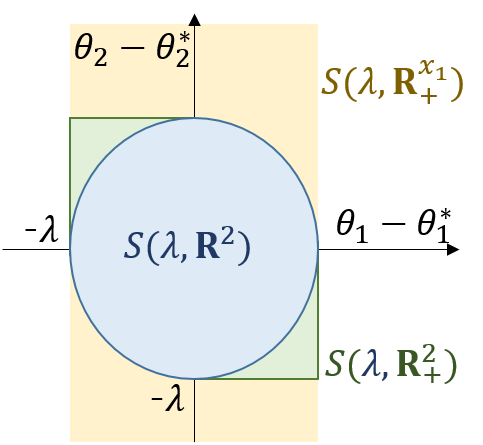
Figure 1 illustrates S⁡(λ,𝒴)=S⁡(λ,𝒴,I2)S(\lambda,\mathcal{Y})=S(\lambda,\mathcal{Y};I_{2}) for 𝒴=𝐑2\mathcal{Y}=\mathbf{R}^{2}, 𝐑+2\mathbf{R}_{+}^{2}, and 𝐑+x1:={(x1,0)⊤∈𝐑2∣x1≥0}\mathbf{R}^{x_{1}}_{+}:=\{(x_{1},0)^{\top}\in\mathbf{R}^{2}\mid x_{1}\geq 0\}, where all these 𝒴\mathcal{Y} include the true optimum solution x∗=(1,0)⊤x^{*}=(1,0)^{\top}. The figure clearly shows that, with a fixed λ\lambda, a smaller 𝒴\mathcal{Y} results in a larger SS:

λ​UΣ∗=S⁡(λ,𝐑2)⊊S⁡(λ,𝐑+2)⊊S⁡(λ,𝐑+x1).\displaystyle\lambda U_{\Sigma^{*}}=S(\lambda,\mathbf{R}^{2})\subsetneq S(\lambda,\mathbf{R}^{2}_{+})\subsetneq S(\lambda,\mathbf{R}^{x_{1}}_{+}).

Recall that Fact 4 and Lemma 5 lead us to define λ\lambda in order to satisfy θ^n−θ∗∈S⁡(λ,𝒴)\hat{\theta}_{n}-\theta^{*}\in S(\lambda,\mathcal{Y}) with desired probability 1−δ1-\delta.

More specifically, let θ^n\hat{\theta}_{n} be distributed by the normal distribution 𝒩⁡(θ∗,I2)\mathcal{N}(\theta^{*},I_{2}) and let δ=0.1\delta=0.1. Fact 4 with UI2(=S⁡(λ,𝐑2))U_{I_{2}}(=S(\lambda,\mathbf{R}^{2})) then requires λ=χ2−1​(1−δ)≈2.1\lambda=\chi_{2}^{-1}(1-\delta)\approx 2.1, while Lemma 5 together with S⁡(λ,𝐑+x1)S(\lambda,\mathbf{R}^{x_{1}}_{+}) requires λ=χ1−1​(1−δ)≈1.6\lambda=\chi_{1}^{-1}(1-\delta)\approx 1.6. Since a smaller λ\lambda yields a closer solution to the optimal one, this indicates the possibility of having a better solution.
Refer to caption
Figure 1: Plot of S⁡(λ,𝒴)=S⁡(λ,𝒴,I2)S(\lambda,\mathcal{Y})=S(\lambda,\mathcal{Y};I_{2}) for 𝒴=𝐑2\mathcal{Y}=\mathbf{R}^{2}, 𝐑+2\mathbf{R}_{+}^{2}, and 𝐑+x1\mathbf{R}^{x_{1}}_{+}, in a two-dimensional toy problem.

∎

For an effective use of Lemma 5, we must be able to evaluate the probability Prob⁡(θ^n−θ∗∈S⁡(λ,𝒴,Σ∗))\mathrm{Prob}(\hat{\theta}_{n}-\theta^{*}\in S(\lambda,\mathcal{Y};\Sigma^{*})) for 𝒴⊆𝒳\mathcal{Y}\subseteq\mathcal{X}, and must find a good subspace 𝒴⊆𝒳\mathcal{Y}\subseteq\mathcal{X} without knowing θ∗\theta^{*} and 𝒫∗\mathcal{P}^{*}.

1.3.2 Probability Evaluation

In order to evaluate probability without θ∗\theta^{*} and 𝒫∗\mathcal{P}^{*}, in Section 3 we characterize S⁡(λ,𝒴,Σ∗)S(\lambda,\mathcal{Y};\Sigma^{*}) as an intersection of Minkovski’s sum of an ellipsoid and a dual cone. Since such an intersection is a convex set, we can apply the high-dimensional Berry-Esseen theorem for convex sets [5] in order to approximate the distribution of θ^n−θ∗\hat{\theta}_{n}-\theta^{*} by a normal distribution while maintaining a theoretical guarantee. We then propose a sampling-based algorithm for measuring the probability with sufficient accuracy.

1.3.3 Subspace Selection

To find good subspace 𝒴⊆𝒳\mathcal{Y}\subseteq\mathcal{X}, in Section 4 we extend the two-step empirical domain reduction algorithm proposed for risk minimization with a single uncertainty objective [16] to our context for robust optimization with multiple uncertain constraints. Such a reduced space must satisfy (6) and (7) in Lemma 5 with high probability. For (6), since the reduction is based on empirical estimate θ^n\hat{\theta}_{n}, the resulting S⁡(λ,𝒴,Σ)S(\lambda,\mathcal{Y};\Sigma) also includes stochastic uncertainty. We must thus avoid over-fitting on a given single sample and keep consistency with other sampling scenarios. In addition, (7) requires that the solution x⁡(λ,θ,Σ)x(\lambda;\theta,\Sigma) must be included in 𝒴\mathcal{Y} without forcing it by adding constraints. These two requirements require precise control of domain reduction, which can be done using our empirical two-step domain reduction algorithm.

1.4 Related studies

Our approach can be summarized in terms of the following concepts: inequality on subspaces, probability evaluation, and subspace selection. While these concepts are novel in the context of robust optimization, they have already been proven to be effective in the context of variance-based regularization for risk minimization in machine learning. Let us note that variance-based regularization regularizes uncertain objectives by means of scaled (square-root of) variance, and thus it is similar to the robust optimization with ellipsoidal uncertainty that introduces redundancy into uncertain constraints, which redundancy is proportional to (square-root of) variance.

In the context of risk minimization, the relationship between the size of an optimization domain and the speed of convergence has been characterized by various complexity measures, such as VC dimension [15], covering number [13], and Rademacher complexity [1]. Studies of variance-based regularization [13, 14] have determined the scale of a regularizer on the basis of these complexity measures in order for a regularized empirical risk function to bound the true objectives with a desired probabilities. A recent study of empirical hypothesis space reduction [16] has achieved, by means of subspace selection, an acceleration of convergence that is asymptotically independent of the dimensionality of uncertain parameters.

To make use of the approaches in [16], which is designed for variance-based regularization, in robust optimization, we have dealt with the issues below. Robust optimization has several uncertain constraints, while risk minimization has a single uncertain objective. In particular, while an uncertainty objective does not influence the feasible domain, uncertain constraints do influence, which increases the difficulty of subspace selection. In addition, in robust optimization, it is often assumed that uncertain functions are linear with respect to uncertain parameters, and this linearity has led us to propose a novel sampling-based evaluation of violation probability.

2 Preliminary

2.1 Technical lemmas

This section introduces a series of lemmas. The following Gershgorin circle theorem characterizes the list of eigenvalues of a matrix A∈𝐑d×dA\in\mathbf{R}^{d\times d} by its elements ai​ja_{ij}.

Lemma 7 (The Gershgorin circle theorem; see [11]).

Let A=(ai​j)∈𝐑d×dA=(a_{ij})\in\mathbf{R}^{d\times d}, and define Ri=∑j≠i|ai​j|R_{i}=\sum_{j\neq i}|a_{ij}|. Under suitable ordering, the set of eigenvalues λ1,…,λd\lambda_{1},\dots,\lambda_{d} of AA satisfy ai​i−Ri≤λi≤ai​i+Ria_{ii}-R_{i}\leq\lambda_{i}\leq a_{ii}+R_{i}.

Hoeffding’s inequality below bounds the gap between sample average and true average.

Lemma 8 (Hoeffding’s inequality; see [9]).

Let Z,Z1,…,ZnZ,Z_{1},\dots,Z_{n} be i.i.d. random variables with values in [0,1][0,1] and let δ>0\delta>0. Then we have

Prob⁡(E⁡[Z]−1n​∑i=1nZi≤log⁡1/δ2​n)≥1−δ,\displaystyle\mathrm{Prob}\left(\mathrm{E}[Z]-\frac{1}{n}\sum_{i=1}^{n}Z_{i}\leq\sqrt{\frac{\log 1/\delta}{2n}}\right)\geq 1-\delta,
Prob⁡(1n​∑i=1nZi−E⁡[Z]≤log⁡1/δ2​n)≥1−δ.\displaystyle\mathrm{Prob}\left(\frac{1}{n}\sum_{i=1}^{n}Z_{i}-\mathrm{E}[Z]\leq\sqrt{\frac{\log 1/\delta}{2n}}\right)\geq 1-\delta.

The following Berry-Esseen theorem enables us to evaluate the speed of convergence of the central limit theorem (for tighter coefficient c1c_{1} in a one-dimensional case, see [12]).

Lemma 9 (The high-dimensional Berry-Esseen inequality [5]).

Let d≥1d\geq 1 be an integer. Let 𝒞d\mathcal{C}_{d} be a set of convex set in 𝐑d\mathbf{R}^{d} and cd:=400​d1/4c_{d}:=400d^{1/4}. Let Z1,…,ZnZ_{1},\dots,Z_{n} be i.i.d. random variables over 𝐑d\mathbf{R}^{d} with E⁡[Zi]=0E[Z_{i}]=0, E⁡[Zi​Zi⊤]=IdE[Z_{i}Z_{i}^{\top}]=I_{d}, and E⁡[‖Zi‖3]≤τE[\|Z_{i}\|^{3}]\leq\tau. Let Z=(1/n)​∑i=1nZiZ=(1/\sqrt{n})\sum_{i=1}^{n}Z_{i}. It then holds that

supC∈𝒞d|ProbW∼𝒩⁡(0,Id)​(W∈C)−Prob𝑍​(Z∈C)|≤cd​τn\displaystyle\sup_{C\in\mathcal{C}_{d}}\left|\underset{W\sim\mathcal{N}(0,I_{d})}{\mathrm{Prob}}(W\in C)-\underset{Z}{\mathrm{Prob}}(Z\in C)\right|\leq\frac{c_{d}\tau}{\sqrt{n}}

2.2 Estimation accuracy

We can show here the accuracy of estimators θ^n\hat{\theta}_{n} and Σ^n\hat{\Sigma}_{n} on the basis of the lemmas introduced in the previous section and the following assumption. Let 𝒫Δ∗\mathcal{P}^{*}_{\Delta} denote the distribution of Δ=Σ∗−1/2(θ−θ∗)\Delta=\Sigma^{*-1/2}(\theta-\theta^{*}) where θ∼𝒫∗\theta\sim\mathcal{P}^{*}.

Assumption 10.

An upper-bound τ\tau of EΔ∼𝒫Δ∗​[‖Δ‖3]E_{\Delta\sim\mathcal{P}^{*}_{\Delta}}[\|\Delta\|^{3}] and τ′\tau^{\prime} of maxj=1,2,…,d⁡EΔ∼𝒫Δ∗​[Δj6]\max_{j=1,2,\dots,d}E_{\Delta\sim\mathcal{P}^{*}_{\Delta}}[\Delta_{j}^{6}] is given.

We here assume that (an upper-bound of) the third moment τ\tau and sixth moment τ′\tau^{\prime} is known, since the speed of convergence is less influenced by the higher-order moments τ\tau and τ′\tau^{\prime} than by the first and second moments (θ∗\theta^{*} and Σ∗\Sigma^{*}). In practice, τ\tau and τ′\tau^{\prime} can be calculated if the domain of the distribution 𝒫∗\mathcal{P}^{*} is bounded, or it can also be estimated using samples θn\theta^{n}.

Under Assumption 10, the distribution of θ^n\hat{\theta}_{n} converges to the normal distribution 𝒩⁡(0,Σ∗/n)\mathcal{N}(0,\Sigma^{*}/n) by the central limit theorem. Recall the definitions of 𝒞d\mathcal{C}_{d} and cd:=400​d1/4c_{d}:=400d^{1/4} in Lemma 9. The speed of convergence can be characterized by τ\tau, τ′\tau^{\prime}, and Lemma 9 as follows:

Lemma 11.

It holds that

supC∈𝒞d|ProbΔ∼𝒩⁡(0,Σ∗/n)​(Δ∈C)−Probθ^n​(θ^n−θ∗∈C)|≤cd​τn.\displaystyle\sup_{C\in\mathcal{C}_{d}}\left|\underset{\Delta\sim\mathcal{N}(0,\Sigma^{*}/n)}{\mathrm{Prob}}(\Delta\in C)-\underset{\hat{\theta}_{n}}{\mathrm{Prob}}(\hat{\theta}_{n}-\theta^{*}\in C)\right|\leq\frac{c_{d}\tau}{\sqrt{n}}.

For δ′>0\delta^{\prime}>0, let us define ηd,n​(δ′)\eta_{d,n}(\delta^{\prime}) by

ηd,n​(δ′):=τ1′/3​dn​χ1−1​(1−δ′d2+c1​τ′n).\displaystyle\eta_{d,n}(\delta^{\prime}):=\frac{\tau^{{}^{\prime}1/3}d}{\sqrt{n}}\chi_{1}^{-1}\left(1-\frac{\delta^{\prime}}{d^{2}}+\frac{c_{1}\tau^{\prime}}{\sqrt{n}}\right).

The relative accuracy of estimator Σ^n\hat{\Sigma}_{n} can be characterized by Lemma 7 and Lemma 9 as follows.

Lemma 12.

For δ′>0\delta^{\prime}>0, the following then holds with probability at least 1−δ′1-\delta^{\prime}:

(1−ηd,n​(δ′))​Σ∗⪯Σ^n⪯(1+ηd,n​(δ′))​Σ∗.\displaystyle\left(1-\eta_{d,n}(\delta^{\prime})\right)\Sigma^{*}\preceq\hat{\Sigma}_{n}\preceq\left(1+\eta_{d,n}(\delta^{\prime})\right)\Sigma^{*}. (10)

Note that the above bound can be improved by using the Berry-Esseen theorem that is specialized for a one-dimensional random variable, rather than by using Lemma 9. Since this improvement does not influence the order of convergence, we here use Lemma 9 for simplicity of presentation.

3 Probability Evaluation Algorithm

This section proposes an algorithm that realizes the concept of probability evaluation discussed in Section 1.3.

3.1 Geometric characterization of S⁡(μ,𝒴,Σ)S(\mu,\mathcal{Y};\Sigma)

Recall that S⁡(λ,𝒴,Σ)⊆𝐑dS(\lambda,\mathcal{Y};\Sigma)\subseteq\mathbf{R}^{d} is the set of estimation error θ−θ∗\theta-\theta^{*} that does not cause a violation of the true constraint over 𝒴\mathcal{Y} with the scale λ\lambda. Here we prove that SS is a convex set for any λ\lambda, 𝒴\mathcal{Y}, and Σ\Sigma.

Since gkg_{k} is linear in θ\theta, there exists a function vk:𝒳→𝐑dv_{k}:\mathcal{X}\to\mathbf{R}^{d} such that

gk​(x,θ)=θ⊤​vk​(x).\displaystyle g_{k}(x,\theta)=\theta^{\top}v_{k}(x).

For 𝒴⊆𝒳\mathcal{Y}\subseteq\mathcal{X}, we define Vk​(𝒴)V_{k}(\mathcal{Y}) by

Vk​(𝒴):={vk​(y)∈𝐑d∣y∈𝒴}.\displaystyle V_{k}(\mathcal{Y}):=\{v_{k}(y)\in\mathbf{R}^{d}\mid y\in\mathcal{Y}\}.

We then define the polar cone Ck+​(𝒴)C_{k}^{+}(\mathcal{Y}) and dual cone Ck−​(𝒴)C_{k}^{-}(\mathcal{Y}) of Vk​(𝒴)V_{k}(\mathcal{Y}) by

Ck+(𝒴):={Δ∈𝐑d∣Δ⊤v≥0,∀v∈Vk(𝒴)},\displaystyle C_{k}^{+}(\mathcal{Y}):=\{\Delta\in\mathbf{R}^{d}\mid\Delta^{\top}v\geq 0,\forall v\in V_{k}(\mathcal{Y})\},
Ck−(𝒴):={Δ∈𝐑d∣Δ⊤v≤0,∀v∈Vk(𝒴)}.\displaystyle C_{k}^{-}(\mathcal{Y}):=\{\Delta\in\mathbf{R}^{d}\mid\Delta^{\top}v\leq 0,\forall v\in V_{k}(\mathcal{Y})\}.

The polar cone Ck+​(𝒴)C_{k}^{+}(\mathcal{Y}) and the dual cone Ck−​(𝒴)C_{k}^{-}(\mathcal{Y}) are convex cones. For a pair of set U,S⊆𝐑dU,S\subseteq\mathbf{R}^{d}, their Minkowski’s sum is defined by U+S:={u+s∣u∈U,s∈S}U+S:=\{u+s\mid u\in U,s\in S\}. Note that Minkowski’s sum of two convex sets is also a convex set. The following theorem characterize S⁡(μ,𝒴,Σ)S(\mu,\mathcal{Y};\Sigma) as an intersection of convex sets:

Lemma 13.

For any λ≥0\lambda\geq 0, 𝒴⊆𝒳\mathcal{Y}\subseteq\mathcal{X}, and Σ⪰0\Sigma\succeq 0, S⁡(λ,𝒴,Σ)S(\lambda,\mathcal{Y};\Sigma) is a convex set. In particular, if gk​(x,θ)g_{k}(x,\theta) is linear in xx for all k=1,2,…,Kk=1,2,\dots,K and 𝒴\mathcal{Y} is convex, then it holds that

S⁡(λ,𝒴,Σ):=(⋂k=1Kλ​UΣ+Ck+​(𝒴))∩(⋂k=1Kλ​UΣ∗+Ck−​(𝒴)).\displaystyle S(\lambda,\mathcal{Y};\Sigma):=\left(\bigcap_{k=1}^{K}\lambda U_{\Sigma}+C_{k}^{+}(\mathcal{Y})\right)\cap\left(\bigcap_{k=1}^{K}\lambda U_{\Sigma^{*}}+C_{k}^{-}(\mathcal{Y})\right).

3.2 Normal approximation via multidimensional Berry-Esseen’ theorem

On the basis of [16, Definition 5], we here introduce the minimum spatial uniform bounds μ⁡(α,𝒴,𝒫,Σ)\mu(\alpha,\mathcal{Y};\mathcal{P},\Sigma) as a minimum scale μ≥0\mu\geq 0 that satisfies (6) with probability α\alpha when θ−θ∗\theta-\theta^{*} is distributed by 𝒫\mathcal{P}:

Definition 14.

Let p∈[0,1]p\in[0,1], 𝒴⊆𝒳\mathcal{Y}\subseteq\mathcal{X}, Σ⪰O\Sigma\succeq O, and 𝒫\mathcal{P} be a distribution over 𝐑d\mathbf{R}^{d}. The minimum spatial uniform bound μ⁡(α,𝒴,𝒫,Σ)∈𝐑+\mu(\alpha,\mathcal{Y};\mathcal{P},\Sigma)\in\mathbf{R}_{+} is defined by:

μ⁡(α,𝒴,𝒫,Σ):=inf{μ≥0∣Probθ∼𝒫​(θ∈S⁡(μ,𝒴,Σ))≥p}.\displaystyle\mu(\alpha,\mathcal{Y};\mathcal{P},\Sigma):=\inf\left\{\mu\geq 0\mid\mathrm{Prob}_{\theta\sim\mathcal{P}}\left(\theta\in S(\mu,\mathcal{Y};\Sigma)\right)\geq p\right\}. (11)

Let us define 𝒫n∗\mathcal{P}^{*}_{n} as the distribution of θ^n−θ∗\hat{\theta}_{n}-\theta^{*}. The ideal goal of this section, then, is to obtain μ⁡(α,𝒴,𝒫n∗,Σ∗)\mu(\alpha,\mathcal{Y};\mathcal{P}^{*}_{n},\Sigma^{*}). μ\mu satisfies the following component-wise monotonicity. Let us denote 𝒩Σ:=𝒩⁡(0,Σ)\mathcal{N}_{\Sigma}:=\mathcal{N}(0,\Sigma).

Lemma 15.

Let p∈[0,1]p\in[0,1], 𝒴⊆𝒳\mathcal{Y}\subseteq\mathcal{X}, Σ⪰O\Sigma\succeq O, and 𝒫\mathcal{P}. Then the following holds.

(i) μ⁡(p,𝒴,𝒫,Σ)≤μ⁡(p′,𝒴,𝒫,Σ)\mu(p,\mathcal{Y};\mathcal{P},\Sigma)\leq\mu(p^{\prime},\mathcal{Y};\mathcal{P},\Sigma) for all p≤p′p\leq p^{\prime}. [Monotonicity in pp]

(ii) μ⁡(p,𝒴,𝒫,Σ)≥μ⁡(p,𝒵,𝒫,Σ)\mu(p,\mathcal{Y};\mathcal{P},\Sigma)\geq\mu(p,\mathcal{Z};\mathcal{P},\Sigma) for all 𝒴⊆𝒵\mathcal{Y}\subseteq\mathcal{Z}. [Reverse Monotonicity in 𝒴\mathcal{Y}]

(iii) μ⁡(p,𝒴,𝒩Σ1,Σ)≥μ⁡(p,𝒴,𝒩Σ2,Σ)\mu(p,\mathcal{Y};\mathcal{N}_{\Sigma_{1}},\Sigma)\geq\mu(p,\mathcal{Y};\mathcal{N}_{\Sigma_{2}},\Sigma) and μ⁡(p,𝒴,𝒫,Σ1)≥μ⁡(p,𝒴,𝒩Σ2,Σ2)\mu(p,\mathcal{Y};\mathcal{P},\Sigma_{1})\geq\mu(p,\mathcal{Y};\mathcal{N}_{\Sigma_{2}},\Sigma_{2}) for all Σ1⪯Σ2\Sigma_{1}\preceq\Sigma_{2}. [Reverse Monotonicity in Σ\Sigma]

(iv) μ⁡(p,𝒴,𝒩ν1​Σ,ν2​Σ)=ν1/ν2​μ​(p,𝒴,𝒩Σ,Σ)\mu(p,\mathcal{Y};\mathcal{N}_{\nu_{1}\Sigma},\nu_{2}\Sigma)=\sqrt{\nu_{1}/\nu_{2}}\mu(p,\mathcal{Y};\mathcal{N}_{\Sigma},\Sigma) for all ν1,ν2>0\nu_{1},\nu_{2}>0. [Scaling]

Recall that Lemma 13 shows the convexity of S⁡(μ,𝒴,Σ)S(\mu,\mathcal{Y};\Sigma) for arbitrary μ\mu, 𝒴\mathcal{Y}, and Σ\Sigma. We can then apply Lemma 11 to bound the gap of probability in (11) for 𝒫n∗\mathcal{P}^{*}_{n} and the corresponding normal 𝒩Σ∗/n\mathcal{N}_{\Sigma^{*}/n}. Combined with the monotonicity shown in Lemma 15 (i), we can upper-bound μ⁡(α,𝒴,𝒫n∗,Σ∗)\mu(\alpha,\mathcal{Y};\mathcal{P}^{*}_{n},\Sigma^{*}) of unknown distribution 𝒫n∗\mathcal{P}^{*}_{n} by its asymptotically normal counterpart:

Proposition 16.

It holds that

1n​μ​(α−cd​τn,𝒴,𝒩Σ∗,Σ∗)≤μ⁡(α,𝒴,𝒫n∗,Σ∗)≤1n​μ​(α+cd​τn,𝒴,𝒩Σ∗,Σ∗).\displaystyle\frac{1}{\sqrt{n}}\mu\left(\alpha-\frac{c_{d}\tau}{\sqrt{n}},\mathcal{Y};\mathcal{N}_{\Sigma^{*}},\Sigma^{*}\right)\leq\mu(\alpha,\mathcal{Y};\mathcal{P}^{*}_{n},\Sigma^{*})\leq\frac{1}{\sqrt{n}}\mu\left(\alpha+\frac{c_{d}\tau}{\sqrt{n}},\mathcal{Y};\mathcal{N}_{\Sigma^{*}},\Sigma^{*}\right).

3.3 Sampling algorithm for calculating spatial uniform bounds for normal distribution

This section fixes p∈[0,1]p\in[0,1], 𝒴⊆𝒳\mathcal{Y}\subseteq\mathcal{X}, and Σ⪰O\Sigma\succeq O, and we then denote μ′​(p)=μ⁡(p,𝒴,𝒩Σ,Σ)\mu^{\prime}(p)=\mu(p,\mathcal{Y};\mathcal{N}_{\Sigma},\Sigma) for notational simplicity. Proposition 16 reduces our goal to that of calculating a minimum spatial uniform bound μ′​(p)\mu^{\prime}(p). Lemma 15 (i) shows that such a μ′\mu^{\prime} is monotone in pp, and μ′\mu^{\prime} satisfies the following property:

Lemma 17.

(i) It holds that χ1−1​(p)≤μ′​(p)≤χd−1​(p)\chi_{1}^{-1}(p)\leq\mu^{\prime}(p)\leq\chi_{d}^{-1}(p).

(ii) It holds that

μ′−1(λ):=ProbΔ∼𝒩Σ(miny∈𝒴⁡λ​rk​(y,Σ)+gk​(y,Δ)≥0,miny∈𝒴⁡λ​rk​(y,Σ)−gk​(y,Δ)≥0,∀k=1,2,…,K).\displaystyle\mu^{{}^{\prime}-1}(\lambda):=\underset{\Delta\sim\mathcal{N}_{\Sigma}}{\mathrm{Prob}}\left(\begin{array}[]{r}\min_{y\in\mathcal{Y}}\lambda r_{k}(y;\Sigma)+g_{k}(y,\Delta)\geq 0,\\ \min_{y\in\mathcal{Y}}\lambda r_{k}(y;\Sigma)-g_{k}(y,\Delta)\geq 0,\\ \forall k=1,2,\dots,K\end{array}\right).

Thus μ′\mu^{\prime} is monotone, upper and lower bounded, and its inverse μ′−1\mu^{{}^{\prime}-1} can be calculated by a series of sampling and optimization. This characterization leads the following algorithm for calculating μ′\mu^{\prime} by sampling from 𝒩Σ\mathcal{N}_{\Sigma} and a binary search, as shown in Algorithm 1.

Given p∈[0,1]p\in[0,1], 𝒴⊆𝒳\mathcal{Y}\subseteq\mathcal{X}, and Σ⪰O\Sigma\succeq O, together with parameters α,β,γ≥0\alpha,\beta,\gamma\geq 0 deciding accuracy, Algorithm 1 calculates a λ\lambda that approximates μ′​(p)\mu^{\prime}(p). Line 1 of the algorithm first defines the number QQ of samples by

Q:=⌈log⁡(2/α)8​β2⌉.\displaystyle Q:=\left\lceil\frac{\log(2/\alpha)}{8\beta^{2}}\right\rceil. (12)

Line 2, then, generates samples εi\varepsilon_{i} for i=1,2,…,Qi=1,2,\dots,Q from the normal distribution 𝒩Σ\mathcal{N}_{\Sigma}. Lines 3–18 estimate μ′​(p)\mu^{\prime}(p) by the binary search. Line 4 defines the upper-bound λ¯\overline{\lambda} and the lower-bound λ¯\underline{\lambda} on the basis of Lemma 17. Line 6 updates λ\lambda as a mean of the upper-bound λ¯\overline{\lambda} and the lower-bound λ¯\underline{\lambda}, and then Lines 7–12 approximately calculate μ′−1(λ)\mu^{{}^{\prime}-1}(\lambda) on the basis of the samples εi\varepsilon_{i} for i=1,2,…,Qi=1,2,\dots,Q and the following lemma:

Lemma 18.

For ε∈𝐑d\varepsilon\in\mathbf{R}^{d}, ε∈S⁡(λ,𝒴,Σ)\varepsilon\in S(\lambda,\mathcal{Y};\Sigma) if and only if ψ⁡(μ,ε)≥0\psi(\mu,\varepsilon)\geq 0, where

ψ⁡(μ,ε):=min⁡{ψ1,+​(ε),ψ1,−​(ε),…,ψK,+​(ε),ψK,−​(ε)}\displaystyle\psi(\mu,\varepsilon):=\min\{\psi_{1,+}(\varepsilon),\psi_{1,-}(\varepsilon),\dots,\psi_{K,+}(\varepsilon),\psi_{K,-}(\varepsilon)\}
where ​ψk,+​(ε):=miny∈𝒴⁡gk​(y,ε)+μ​rk​(y,Σ),\displaystyle\text{ where }\psi_{k,+}(\varepsilon):=\min_{y\in\mathcal{Y}}g_{k}(y,\varepsilon)+\mu r_{k}(y;\Sigma),
ψk,−​(ε):=miny∈𝒴⁡gk​(y,−ε)+μ​rk​(y,Σ).\displaystyle\psi_{k,-}(\varepsilon):=\min_{y\in\mathcal{Y}}g_{k}(y,-\varepsilon)+\mu r_{k}(y;\Sigma). (13)

For each εi\varepsilon_{i}, Line 8 calculates the optimization problem (13) for ε=εi\varepsilon=\varepsilon_{i}, and then Lines 9–11 approximately calculate μ′−1(λ)\mu^{{}^{\prime}-1}(\lambda) by counting the number of such εi∈S⁡(λ,𝒴,Σ)\varepsilon_{i}\in S(\lambda,\mathcal{Y};\Sigma) for i=1,2,…,Qi=1,2,\dots,Q. Note that some of the calculation of ψ⁡(λ,εi)\psi(\lambda,\varepsilon_{i}) can be omitted in practice since ψ⁡(λ,εi)\psi(\lambda,\varepsilon_{i}) is monotonically increasing in λ\lambda. Lines 13–17 update the upper-bound λ¯\overline{\lambda} or the lower-bound λ¯\underline{\lambda} on the basis of the approximate probability qq of μ′−1(λ)\mu^{{}^{\prime}-1}(\lambda). Finally, Line 19 outputs the approximate upper-bound μ˙=λ¯\dot{\mu}=\overline{\lambda} of μ′​(p)\mu^{\prime}(p).

Algorithm 1 Estimation of μ⁡(p,𝒴,𝒩Σ,Σ)\mu(p,\mathcal{Y};\mathcal{N}_{\Sigma},\Sigma)
0:  pp, 𝒴\mathcal{Y}, Σ\Sigma, and accuracy parameter (α,β,γ)(\alpha,\beta,\gamma).
0:  An estimate μ˙\dot{\mu} of μ′​(p,𝒴,𝒩Σ,Σ)\mu^{\prime}(p,\mathcal{Y};\mathcal{N}_{\Sigma},\Sigma)
1:  Define the number of sample QQ by (12).
2:  Sample εi∼𝒩⁡(0,Σ)\varepsilon_{i}\sim\mathcal{N}(0,\Sigma) for i=1,2,…,Qi=1,2,\dots,Q.
3:  # Binary search
4:  Initialize λ¯=χ1−1​(p)\underline{\lambda}=\chi_{1}^{-1}(p), λ¯=χd−1​(p)\overline{\lambda}=\chi_{d}^{-1}(p)
5:  while λ¯−λ¯≥γ\overline{\lambda}-\underline{\lambda}\geq\gamma do
6:   Put λ=(λ¯+λ¯)/2\lambda=(\underline{\lambda}+\overline{\lambda})/2 and initialize q=0q=0
7:   for i=1,2,…,Q do
8:    Solve (13) and obtain ψ⁡(μ,εi)\psi(\mu,\varepsilon_{i}).
9:    if ψ⁡(μ,εi)≥0\psi(\mu,\varepsilon_{i})\geq 0 then
10:     q=q+1/Qq=q+1/Q
11:    end if
12:   end for
13:   if q≥p+(β/2)q\geq p+(\beta/2) then
14:    Put λ¯=λ\underline{\lambda}=\lambda.
15:   else
16:    Put λ¯=λ\overline{\lambda}=\lambda.
17:   end if
18:  end while
19:  Output μ˙=λ¯\dot{\mu}=\overline{\lambda}

This output μ˙\dot{\mu} satisfies the following probabilistic guarantee.

Proposition 19.

With probability at least 1−α1-\alpha, the output μ˙\dot{\mu} of Algorithm 1 satisfy

μ′​(p)≤μ˙≤μ′​(p+β)+γ.\displaystyle\mu^{\prime}(p)\leq\dot{\mu}\leq\mu^{\prime}(p+\beta)+\gamma.

The computational tractability of Algorithm 1 relies heavily on the choice of 𝒴\mathcal{Y}, and this is discussed in the next section, which utilizes Algorithm 1.

4 Empirical Domain Reduction

This section presents an algorithm that achieves our main theoretical result via the concept of subspace selection discussed in Section 1.3.

4.1 Two-step domain reduction algorithm

Let us define constants αn,βn,γn,ηn,δn>0\alpha_{n},\beta_{n},\gamma_{n},\eta_{n},\delta_{n}>0 and empirically reduced domain 𝒴^​(w,μ)\hat{\mathcal{Y}}(w,\mu) for w,μ≥0w,\mu\geq 0 by

αn=δn,βn=cd​τn,γn=1n,\displaystyle\alpha_{n}=\frac{\delta}{\sqrt{n}},\quad\beta_{n}=\frac{c_{d}\tau}{\sqrt{n}},\quad\gamma_{n}=\frac{1}{\sqrt{n}},
ηn:=ηn,d​(d2​c1​τ′n),\displaystyle\eta_{n}:=\eta_{n,d}\left(\frac{d^{2}c_{1}\tau^{\prime}}{\sqrt{n}}\right),
δn:=1n​(2​d2​c1​τ′+4​cd​τ+δ),\displaystyle\delta_{n}:=\frac{1}{\sqrt{n}}\left(2d^{2}c_{1}\tau^{\prime}+4c_{d}\tau+\delta\right),
𝒴^(w,μ):={y∈𝒳|f⁡(y)≤w,gk​(y,θ^)≥−μ​rk​(y,Σ^),k=1,2,…,K}.\displaystyle\hat{\mathcal{Y}}(w,\mu):=\left\{y\in\mathcal{X}\left|\begin{array}[]{l}f(y)\leq w,\\ g_{k}(y,\hat{\theta})\geq-\mu r_{k}(y;\hat{\Sigma}),\\ k=1,2,\dots,K\end{array}\right\}\right..

We can then propose Algorithm 2 for the calculation of the scale λ^\hat{\lambda} of robustness. Lines 1–4 represent the first stage of this algorithm, which conducts subspace selection. Line 1 first calculates coefficient μ˙\dot{\mu} using Algorithm 1 with 𝒴=𝒳\mathcal{Y}=\mathcal{X}. Line 2 defines μ^\hat{\mu} by scaling μ˙\dot{\mu}, and then Line 3 calculates optimum value w^=f​(x^​(3​μ^))\hat{w}=f(\hat{x}(3\hat{\mu})) by solving (1.1) on the basis of scale μ^\hat{\mu}. Line 4 conduct subspace selection by defining 𝒴^=𝒴^​(w^,μ^/(1−ηn))\hat{\mathcal{Y}}=\hat{\mathcal{Y}}(\hat{w},\hat{\mu}/(1-\eta_{n})). Lines 5–6 represent the second stage of the algorithm, which calculates scale λ^\hat{\lambda} on the basis of the subspace 𝒴^\hat{\mathcal{Y}}. Line 5 calculates λ˙\dot{\lambda} using Algorithm 1 with 𝒴=𝒴^\mathcal{Y}=\hat{\mathcal{Y}}, and Line 6 then outputs λ^\hat{\lambda} which defined by scaling λ˙\dot{\lambda}.

Algorithm 2 Computation of empirical scale λ^\hat{\lambda} for minimizing VaRα\mathrm{VaR}_{\alpha}
0:  δ\delta, θ^n\hat{\theta}_{n}, Σ^n\hat{\Sigma}_{n}
0:  x∈𝒳x\in\mathcal{X}
1:  Calculate μ˙\dot{\mu} with Algorithm 1 with inputs p=1−2​cd​τ/np=1-2c_{d}\tau/\sqrt{n}, 𝒴=𝒳\mathcal{Y}=\mathcal{X}, Σ=Σ^n\Sigma=\hat{\Sigma}_{n}, and (α,β,γ)=(αn,βn,γn)(\alpha,\beta,\gamma)=(\alpha_{n},\beta_{n},\gamma_{n})
2:  Define μ^=(1+ηn)​μ˙/(1−ηn)2​n\hat{\mu}=(1+\eta_{n})\dot{\mu}/(1-\eta_{n})^{2}\sqrt{n}
3:  Calculate w^=f​(x^​(3​μ^))\hat{w}=f(\hat{x}(3\hat{\mu}))
4:  Define 𝒴^:=𝒴^​(w^,μ^/(1−ηn))\hat{\mathcal{Y}}:=\hat{\mathcal{Y}}(\hat{w},\hat{\mu}/(1-\eta_{n}))
5:  Calculate λ˙\dot{\lambda} with Algorithm 1 with inputs p=1−δ+δnp=1-\delta+\delta_{n}, 𝒴=𝒴^\mathcal{Y}=\hat{\mathcal{Y}}, Σ=Σ^n\Sigma=\hat{\Sigma}_{n}, and (α,β,γ)=(αn,βn,γn)(\alpha,\beta,\gamma)=(\alpha_{n},\beta_{n},\gamma_{n})
6:  Output λ^:=λ˙/(1−γn)​n\hat{\lambda}:=\dot{\lambda}/(1-\gamma_{n})\sqrt{n}.

4.2 Theoretical analysis

Let n0n_{0} be the minimum integer nn that satisfies

(1+ηn)2(1−ηn)2​μ​(1−δ+δn,𝒳,𝒩Σ∗,Σ∗)+1+ηn(1−ηn)​n≤μ⁡(1−2​cd​τ/n,𝒳,𝒩Σ∗,Σ∗)\displaystyle\frac{(1+\eta_{n})^{2}}{(1-\eta_{n})^{2}}\mu(1-\delta+\delta_{n},\mathcal{X},\mathcal{N}_{\Sigma^{*}},\Sigma^{*})+\frac{1+\eta_{n}}{(1-\eta_{n})\sqrt{n}}\leq\mu(1-2c_{d}\tau/\sqrt{n},\mathcal{X},\mathcal{N}_{\Sigma^{*}},\Sigma^{*})

Note that such n0n_{0} must exist since δn,ηn=O⁡(1/n)\delta_{n},\eta_{n}=O(1/\sqrt{n}). Our main theoretical result can then be given as follows:

Theorem 20.

Suppose that n≥n0n\geq n_{0}, and limε→+0𝒴∗​(f⁡(x∗​(0))+ε,ε)={x∗​(0)}\lim_{\varepsilon\to+0}\mathcal{Y}^{*}(f(x^{*}(0))+\varepsilon,\varepsilon)=\{x^{*}(0)\}. Then the output λ^\hat{\lambda} of Algorithm 2 satisfies

VaRδ​[f∗​(x^n​(λ^))]≤f⁡(x∗​(λ¯n))\displaystyle\mathrm{VaR}_{\delta}[f^{*}(\hat{x}_{n}(\hat{\lambda}))]\leq f(x^{*}(\overline{\lambda}_{n})) (14)

where

limn→∞n​λ¯n≤χ1−1​(1−δ/K).\displaystyle\lim_{n\to\infty}\sqrt{n}\overline{\lambda}_{n}\leq\chi_{1}^{-1}(1-\delta/K). (15)

Thus, under the uniqueness of the true optimum solution x∗​(0)x^{*}(0), the estimated scale λ^\hat{\lambda} is asymptotically independent of the dimension dd.

The essence of the proof of this statement lies in finding subspaces 𝒴¯n,𝒴¯n⊆𝒳\underline{\mathcal{Y}}_{n},\overline{\mathcal{Y}}_{n}\subseteq\mathcal{X} that satisfy the following two conditions: (i) with high probability, it holds that

x^​(λn),x∗​(2​λn)∈𝒴¯n⊆𝒴^⊆𝒴¯n,\displaystyle\hat{x}(\lambda_{n}),x^{*}(2\lambda_{n})\in\underline{\mathcal{Y}}_{n}\subseteq\hat{\mathcal{Y}}\subseteq\overline{\mathcal{Y}}_{n},

and (ii) limn→∞𝒴¯n={x∗​(0)}\lim_{n\to\infty}\overline{\mathcal{Y}}_{n}=\{x^{*}(0)\}. Property (i), together with Lemma 5, implies contribution to proof of (14), and the property (ii) implies asymptotic convergence (15). Since 𝒴^\hat{\mathcal{Y}} is controlled by the estimated optimum value w^\hat{w}, for the existence of both 𝒴¯n\underline{\mathcal{Y}}_{n} and 𝒴¯n\overline{\mathcal{Y}}_{n}, we need to control the range of estimated optimum value w^\hat{w}. We utilize the following lemma for this control:

Lemma 21.

Let μ≥0\mu\geq 0 and κ≥1\kappa\geq 1. Suppose that θ∈𝐑d\theta\in\mathbf{R}^{d}, Σ⪰O\Sigma\succeq O, and 𝒴⊆𝐑d\mathcal{Y}\subseteq\mathbf{R}^{d} satisfy

θ−θ∗∈S⁡(μ,𝒴,Σ),\displaystyle\theta-\theta^{*}\in S(\mu,\mathcal{Y};\Sigma),
x⁡((κ−1)​μ,θ∗,Σ),x⁡(κ​μ,θ,Σ),x⁡((κ+1)​μ,θ∗,Σ)∈𝒴.\displaystyle x((\kappa-1)\mu;\theta^{*},\Sigma),x(\kappa\mu;\theta,\Sigma),x((\kappa+1)\mu;\theta^{*},\Sigma)\in\mathcal{Y}.

It then holds that f∗​(x⁡((κ−1)​μ,θ∗,Σ))≤f∗​(x⁡(κ​μ,θ,Σ))≤f∗​(x⁡((κ+1)​μ,θ∗,Σ))f^{*}(x((\kappa-1)\mu;\theta^{*},\Sigma))\leq f^{*}(x(\kappa\mu;\theta,\Sigma))\leq f^{*}(x((\kappa+1)\mu;\theta^{*},\Sigma)).

Roughly speaking, we bound the range of w^\hat{w} in probability by applying Lemma 21 with κ=3\kappa=3 and μ=μ^\mu=\hat{\mu}.

Let us conclude this section with a brief discussion of the computational tractability of our algorithms.

Remark 22.

Algorithm 2 mainly consists of an optimization (3) in Line 3 and two applications of Algorithm 2 in Lines 1 and 5, where each application consists of O⁡(n​log2​n)O(n\log^{2}n) optimization of (13). If the original robust optimization (3) is a convex programming problem, then (13) with 𝒴=𝒳\mathcal{Y}=\mathcal{X} is a series of KK convex programmings. It is thus natural to assume that Lines 1 and 3 are computationally tractable.

For the second application of Algorithm 1, in Line 5, note that the subspace 𝒴=𝒴^\mathcal{Y}=\hat{\mathcal{Y}} will not generally be convex because of the concavity of −rk-r_{k}. In practical implementation, we can replace rkr_{k} in the definition of 𝒴^​(w,μ)\hat{\mathcal{Y}}(w,\mu) by an upper-bound uku_{k} that makes 𝒴^\hat{\mathcal{Y}} convex. If such a uku_{k} can be bounded above as uk​(x,Σ)≤κ​rk​(x,Σ)u_{k}(x;\Sigma)\leq\kappa r_{k}(x;\Sigma) with some constant κ≥1\kappa\geq 1, then the resulting output λ^\hat{\lambda} of Algorithm 2 will also satisfy the guarantee in Theorem 20.

Let us introduce a simple example of such an upper-bound uku_{k}. Suppose that 𝒳\mathcal{X} is the positive orthant (𝒳=𝐑+d\mathcal{X}=\mathbf{R}^{d}_{+}) and that gk​(x,θ)=θ⊤​xg_{k}(x,\theta)=\theta^{\top}x. Then rk​(x,Id)=‖x‖2r_{k}(x,I_{d})=\|x\|_{2}, where ∥⋅∥q\|\cdot\|_{q} is the ℓq\ell_{q}-norm for q≥0q\geq 0. It then holds that rk​(x,Id)≤d​‖x‖1r_{k}(x,I_{d})\leq\sqrt{d}\|x\|_{1}. Observe that ∥⋅∥1\|\cdot\|_{1} is linear on the positive orthant 𝒳\mathcal{X}, and thus this uku_{k} is computationally tractable.

5 Experiments

Refer to caption
Figure 2: Value-at-risk VaR⁡[f∗​(x^n​(λ))]\mathrm{VaR}[f^{*}(\hat{x}_{n}(\lambda))] for scale λ\lambda. The vertical line shows the value-at-risk, and the horizontal line shows the number of samples. Respective yellow, green, blue lines show the result with λ=χ1−1​(1−δ)\lambda=\chi_{1}^{-1}(1-\delta), χd−1​(1−δ)\chi_{d}^{-1}(1-\delta), and λ^n\hat{\lambda}_{n}.
Refer to caption
Figure 3: Scale of robustness λ\lambda. Vertical line shows the value of scale of robustness λ\lambda, and the horizontal line shows the number of samples. Respective yellow, green, blue lines indicate the value of λ=χ1−1​(1−δ)\lambda=\chi_{1}^{-1}(1-\delta), χd−1​(1−δ)\chi_{d}^{-1}(1-\delta), and n​λ^n\sqrt{n}\hat{\lambda}_{n}.

5.1 Experimental setting

Let us consider the following simple portfolio optimization problem, which has been examined by several existing studies in robust optimization [8, 3]. Suppose that there are dd items whose costs are θ1,…,θd\theta_{1},\dots,\theta_{d}, which are uncertain parameters. The task is to find a convex combination (portfolio) that minimizes the cost:

min∑i=1dθixis.t. ∑i=1dxi≤1,xi≥0,i=1,…,d.\displaystyle\begin{array}[]{ll}&\displaystyle\min\sum_{i=1}^{d}\theta_{i}x_{i}\\ &\text{s.t. }\displaystyle\sum_{i=1}^{d}x_{i}\leq 1,\quad x_{i}\geq 0,\ \ i=1,\dots,d.\end{array}

This problem has an uncertain objective function. Thus, we first translate this problem into the our setting (1.1). Let us introduce an additional variable x0x_{0}. We denote by xx the set of variables x=(x0,x1,…,xd)x=(x_{0},x_{1},\dots,x_{d}) over 𝐑d+1\mathbf{R}^{d+1}. We also introduce a dummy parameter θ0=1\theta_{0}=1. We define 𝒳\mathcal{X}, ff, and gg by

𝒳\displaystyle\mathcal{X} :={x∈𝐑d+1|∑i=1dxi≤1xi≥0,i=1,2,…,d.},\displaystyle:=\left\{x\in\mathbf{R}^{d+1}\left|\begin{array}[]{l}\sum_{i=1}^{d}x_{i}\leq 1\\ x_{i}\geq 0,\quad i=1,2,\dots,d.\end{array}\right\},\right.
f⁡(x)\displaystyle f(x) :=x0,\displaystyle:=x_{0},
g⁡(x,θ)\displaystyle g(x,\theta) :=θ0​x0−∑i=1dθi​xi.\displaystyle:=\theta_{0}x_{0}-\sum_{i=1}^{d}\theta_{i}x_{i}.

Then the portfolio optimization problem (5.1) is captured by our setting (1.1).

For this problem, we generate synthetic data as follows. We fix δ=0.3\delta=0.3, d=20d=20, and θ∗=(−1,−0.9,−0.8,…,0.8,0.9)⊤\theta^{*}=(-1,-0.9,-0.8,\dots,0.8,0.9)^{\top}. We set the covariance matrix Σ∗\Sigma^{*} as a diagonal matrix Σ∗=diag⁡(σ12,σ22,…,σd2)\Sigma^{*}=\mathrm{diag}(\sigma_{1}^{2},\sigma_{2}^{2},\dots,\sigma_{d}^{2}) where σi\sigma_{i} follows a uniform distribution over [0,10][0,10]. For each sample size nn and true covariance matrix, we generate 2020 sets of nn i.i.d. samples from 𝒩⁡(θ∗,Σ∗)\mathcal{N}(\theta^{*},\Sigma^{*}), over which samples value-at-risk will be approximately calculated. All our experimental results are average over 3030 generation of such covariance matrix Σ∗\Sigma^{*}. For a solution x^\hat{x} that does not satisfy the true constraint, we put f∗​(x^)=1f^{*}(\hat{x})=1 instead of f∗​(x^)=∞f^{*}(\hat{x})=\infty for the purpose of clear visualization.

To make Algorithm 2 practical, we applied the following approximations: While we bound the gap of the probability mass of the true distribution of θ^n−θ∗\hat{\theta}_{n}-\theta^{*} and 𝒩Σ∗/n\mathcal{N}_{\Sigma^{*}/n} by cd​τ/nc_{d}\tau/\sqrt{n} in our theoretical analysis, we simply replace the true distribution by its normal estimate 𝒩Σ^n/n\mathcal{N}_{\hat{\Sigma}_{n}/n} in implementation by putting cd=τ=0c_{d}=\tau=0. Also, our theoretical analysis carefully replace the true covariance matrix Σ∗\Sigma^{*} by its probabilistic upper-bound Σ^n/(1−ηn)\hat{\Sigma}_{n}/(1-\eta_{n}) or lower-bound Σ^n/(1+ηn)\hat{\Sigma}_{n}/(1+\eta_{n}), but we simply replace Σ∗\Sigma^{*} by Σ^n\hat{\Sigma}_{n} in implementation by putting τ′=0\tau^{\prime}=0.

5.2 Experimental results

We solved the robust optimization problem (1.1) for three different λ\lambda:

  • •

    [proposed] λ=λ^n\lambda=\hat{\lambda}_{n} calculated by Algorithm 2,

  • •

    [lower-bound] λ=λ¯:=χ1−1​(1−δ)/n\lambda=\underline{\lambda}:=\chi_{1}^{-1}(1-\delta)/\sqrt{n}. This is a lower-bound in terms of Lemma 17.

  • •

    [upper bound] λ=λ¯:=χd−1​(1−δ)/n\lambda=\overline{\lambda}:=\chi_{d}^{-1}(1-\delta)/\sqrt{n}. This is the the scale adopted by the standard approach on the basis of Fact 4.

Figure 3 shows the value-at-risk VaRδ​[f∗​(x^​(λ))]\mathrm{VaR}_{\delta}[f^{*}(\hat{x}(\lambda))] for each λ\lambda. We observed that

  • •

    The lower-bound λ¯\underline{\lambda} (yellow) showed worst performance with small sample size n≤60n\leq 60. This performance is due to the violation of true constraints with probability more than δ\delta. Although this λ¯\underline{\lambda} showed the best performance with large sample size n≥120n\geq 120, this scale is inadequate for guaranteed optimization.

  • •

    The upper-bound λ¯\overline{\lambda} (green) could always satisfy the true constraint with designed probability 1−δ1-\delta, but showed the worst speed of convergence. This shows that λ¯\overline{\lambda} is too conservative.

  • •

    The proposed method λ^n\hat{\lambda}_{n} (blue) showed the best performance with wide range of sample size 20≤n≤12020\leq n\leq 120. This can always satisfy the true constraint, and, at the same time, showed rather speedy convergence than λ¯\overline{\lambda}.

We next observe the convergence of the scale n​λ^n\sqrt{n}\hat{\lambda}_{n} to χ1−1​(1−δ)\chi_{1}^{-1}(1-\delta), which is proven by Theorem 20. Figure 3 show the value n​λ^n\sqrt{n}\hat{\lambda}_{n} (blue) in comparison with its lower-bound χ1−1​(1−δ)\chi_{1}^{-1}(1-\delta) (yellow) and upper-bound χd−1​(1−δ)\chi_{d}^{-1}(1-\delta) (green). The scale n​λ^n\sqrt{n}\hat{\lambda}_{n} is about χ4−1​(1−δ)≈2.2\chi_{4}^{-1}(1-\delta)\approx 2.2 with small samples n≤200n\leq 200, and this implies that our algorithm succeeded in selecting four dimensional subspace. The scale n​λ^n\sqrt{n}\hat{\lambda}_{n} decreased to χ2−1​(1−δ)≈1.55\chi_{2}^{-1}(1-\delta)\approx 1.55 with n=1000n=1000, and then slowly converged to χ1−1​(1−δ)\chi_{1}^{-1}(1-\delta).

6 Concluding remarks

This paper has shown that the scale of robustness required for achieving a given confidence probability is dependent on the size of optimization domain, and then has proposed an algorithm for deciding the scale tightly on the basis of empirical domain reduction. The analysis has proven that the scale is asymptotically independent of the parameter dimension, and our experiments has demonstrated that the proposed method can achieve better performance while maintaining probabilistic guarantee.

References

  • [1] Peter L Bartlett and Shahar Mendelson. Rademacher and gaussian complexities: Risk bounds and structural results. Journal of Machine Learning Research, 3(Nov):463–482, 2002.
  • [2] A. Ben-Tal, L. El Ghaoui, and A. Nemirovski. Robust optimization. Princeton University Press, 2009.
  • [3] A. Ben-Tal and A. Nemirovski. Robust solutions of uncertain linear programs. Operations research letters, 25(1):1–13, 1999.
  • [4] Aharon Ben-Tal, Dick Den Hertog, Anja De Waegenaere, Bertrand Melenberg, and Gijs Rennen. Robust solutions of optimization problems affected by uncertain probabilities. Management Science, 59(2):341–357, 2013.
  • [5] Vidmantas Bentkus. On the dependence of the berry–esseen bound on dimension. Journal of Statistical Planning and Inference, 113(2):385–402, 2003.
  • [6] Dimitris Bertsimas, David B Brown, and Constantine Caramanis. Theory and applications of robust optimization. SIAM review, 53(3):464–501, 2011.
  • [7] Dimitris Bertsimas, Vishal Gupta, and Nathan Kallus. Data-driven robust optimization. Mathematical Programming, 167(2):235–292, 2018.
  • [8] Dimitris Bertsimas and Melvyn Sim. The price of robustness. Operations research, 52(1):35–53, 2004.
  • [9] Stéphane Boucheron, Gábor Lugosi, and Pascal Massart. Concentration inequalities: A nonasymptotic theory of independence. Oxford university press, 2013.
  • [10] Erick Delage and Yinyu Ye. Distributionally robust optimization under moment uncertainty with application to data-driven problems. Operations research, 58(3):595–612, 2010.
  • [11] Gene H Golub and Charles F Van Loan. Matriz computations. The Johns Hopkins University Press, Baltimore, USA, 1989.
  • [12] V Yu Korolev and Irina G Shevtsova. On the upper bound for the absolute constant in the berry–esseen inequality. Theory of Probability & Its Applications, 54(4):638–658, 2010.
  • [13] A Maurer and M Pontil. Empirical bernstein bounds and sample variance penalization. In COLT 2009-The 22nd Conference on Learning Theory, 2009.
  • [14] Hongseok Namkoong and John C Duchi. Variance-based regularization with convex objectives. In Advances in Neural Information Processing Systems, pages 2975–2984, 2017.
  • [15] VN Vapnik and A Ya Chervonenkis. On the uniform convergence of relative frequencies of events to their probabilities. Theory of Probability and its Applications, 16(2):264, 1971.
  • [16] Akihiro Yabe and Takanori Maehara. Empirical hypothesis space reduction. arXiv preprint, https://arxiv.org/abs/1909.01576, 2019.

Appendix A Proofs

A.1 Proofs for the statements in Section 1

Proof of Fact 4.

By θ−θ∗∈λ​UΣ\theta-\theta^{*}\in\lambda U_{\Sigma}, for any x∈𝒳x\in\mathcal{X} and k=1,2,…,Kk=1,2,\dots,K, it holds that

minu∈UΣ⁡gk​(x,θ∗+2​λ​u)≤minu∈UΣ⁡gk​(x,θ+λ​u)≤gk​(x,θ∗).\displaystyle\min_{u\in U_{\Sigma}}g_{k}(x,\theta^{*}+2\lambda u)\leq\min_{u\in U_{\Sigma}}g_{k}(x,\theta+\lambda u)\leq g_{k}(x,\theta^{*}).

The left inequality implies that f⁡(x⁡(λ,θ,Σ))≤f⁡(x⁡(2​λ,θ∗,Σ))f(x(\lambda;\theta,\Sigma))\leq f(x(2\lambda;\theta^{*},\Sigma)), and the right inequality implies that f∗​(x⁡(λ,θ,Σ))<∞f^{*}(x(\lambda;\theta,\Sigma))<\infty. It thus holds that f∗​(x⁡(λ,θ,Σ))≤f∗​(x⁡(2​λ,θ∗,Σ))f^{*}(x(\lambda;\theta,\Sigma))\leq f^{*}(x(2\lambda;\theta^{*},\Sigma)). ∎

Proof of Proposition 2.

Since θ^n−θ∗∈λ​UΣ∗\hat{\theta}_{n}-\theta^{*}\in\lambda U_{\Sigma^{*}} with probability at least 1−δ1-\delta, it holds that

VaRδ​[f∗​(x⁡(λ,θ^n,Σ∗))]\displaystyle\mathrm{VaR}_{\delta}[f^{*}(x(\lambda;\hat{\theta}_{n},\Sigma^{*}))] ≤maxθ:θ−θ∗∈λ​UΣ∗f∗(x(λ;θ,Σ∗))\displaystyle\leq\max_{\theta:\theta-\theta^{*}\in\lambda U_{\Sigma^{*}}}f^{*}(x(\lambda;\theta,\Sigma^{*}))
≤f∗​(x∗​(2​λ)).\displaystyle\leq f^{*}(x^{*}(2\lambda)).

The last inequality follows from Fact 4. ∎

Proof of Lemma 5.

By the definition of rkr_{k} and S⁡(λ,𝒴,Σ)S(\lambda,\mathcal{Y};\Sigma) and linearlity of gkg_{k} with respect to θ\theta, for all y∈𝒴y\in\mathcal{Y}, it holds that

minu∈UΣ⁡gk​(y,θ∗+2​λ​u)\displaystyle\min_{u\in U_{\Sigma}}g_{k}(y,\theta^{*}+2\lambda u) =gk​(y,θ)−gk​(y,θ∗−θ)−2​λ​rk​(y,Σ)\displaystyle=g_{k}(y,\theta)-g_{k}(y,\theta^{*}-\theta)-2\lambda r_{k}(y;\Sigma)
≤minu∈UΣ⁡gk​(y,θ+λ​u)\displaystyle\leq\min_{u\in U_{\Sigma}}g_{k}(y,\theta+\lambda u)
=gk​(y,θ∗)+gk​(y,θ−θ∗)−λ​rk​(y,Σ)\displaystyle=g_{k}(y,\theta^{*})+g_{k}(y,\theta-\theta^{*})-\lambda r_{k}(y;\Sigma)
≤gk​(y,θ∗).\displaystyle\leq g_{k}(y,\theta^{*}).

Since x⁡(λ,θ,Σ),x⁡(2​λ,θ∗,Σ)∈𝒴x(\lambda;\theta,\Sigma),x(2\lambda;\theta^{*},\Sigma)\in\mathcal{Y}, it holds that f∗​(x⁡(λ,θ,Σ)),f∗​(x⁡(2​λ,θ∗,Σ))<∞f^{*}(x(\lambda;\theta,\Sigma)),f^{*}(x(2\lambda;\theta^{*},\Sigma))<\infty. By the first inequality and the optimality of x⁡(λ,θ,Σ)x(\lambda;\theta,\Sigma) over 𝒳\mathcal{X}, then, we have f⁡(x⁡(λ,θ,Σ))≤f⁡(y)f(x(\lambda;\theta,\Sigma))\leq f(y) that satisfies y∈𝒴y\in\mathcal{Y} and minu∈UΣ⁡gk​(y,θ∗+2​λ​u)≥0\min_{u\in U_{\Sigma}}g_{k}(y,\theta^{*}+2\lambda u)\geq 0. Thus the statement holds. ∎

A.2 Proofs for the statements in Section 2

For each θi∼𝒫∗\theta^{i}\sim\mathcal{P}^{*} for i=1,2,…,ni=1,2,\dots,n, let us denote Δi=Σ∗−1/2(θi−θ∗)\Delta^{i}=\Sigma^{*-1/2}(\theta^{i}-\theta^{*}) and Δn=∑i=1nΔi/n\Delta_{n}=\sum_{i=1}^{n}\Delta^{i}/\sqrt{n}. Then each Δi\Delta^{i} is distributed by 𝒫Δ∗\mathcal{P}_{\Delta}^{*}.

Proof of Lemma 11.

Observe that each Δi\Delta^{i} satisfies E⁡[Δi]=0E[\Delta^{i}]=0, E⁡[Δi​Δi⊤]=IdE[\Delta^{i}\Delta^{i\top}]=I_{d}, and E⁡[‖Δi‖3]≤τE[\|\Delta^{i}\|^{3}]\leq\tau by Assumption 10. Lemma 9 implies that

supC∈𝒞d|ProbW∼𝒩⁡(0,Id)​(W∈C)−ProbΔn​(Δn∈C)|≤cd​τn.\displaystyle\sup_{C\in\mathcal{C}_{d}}\left|\underset{W\sim\mathcal{N}(0,I_{d})}{\mathrm{Prob}}(W\in C)-\underset{\Delta_{n}}{\mathrm{Prob}}(\Delta_{n}\in C)\right|\leq\frac{c_{d}\tau}{\sqrt{n}}.

Mapping both random variables as W↦(Σ∗/n)1/2​WW\mapsto(\Sigma^{*}/n)^{1/2}W and Δn↦(Σ∗/n)1/2​Δn=θ^n\Delta_{n}\mapsto(\Sigma^{*}/n)^{1/2}\Delta_{n}=\hat{\theta}_{n}, we have the statement. ∎

Proof of Lemma 12.

Let us define I^n:=(1/n)​∑i=1nΔi​Δi⊤\hat{I}_{n}:=(1/n)\sum_{i=1}^{n}\Delta^{i}\Delta^{i\top}. Since Σ1/2​I^n​Σ1/2=Σ^n\Sigma^{1/2}\hat{I}_{n}\Sigma^{1/2}=\hat{\Sigma}_{n} and the relationship O⪯Σ1⪯Σ2O\preceq\Sigma_{1}\preceq\Sigma_{2} of positive semidefinit matrices is invariant under the mapping Σ1↦Σ1/2​Σ1​Σ1/2\Sigma_{1}\mapsto\Sigma^{1/2}\Sigma_{1}\Sigma^{1/2} by another positive semidefinite matrix Σ\Sigma, it is enough to prove that

(1−cd​τn)​Id⪯I^n⪯(1+cd​τn)​Id.\displaystyle\left(1-\frac{c_{d}\tau}{\sqrt{n}}\right)I_{d}\preceq\hat{I}_{n}\preceq\left(1+\frac{c_{d}\tau}{\sqrt{n}}\right)I_{d}. (18)

For each i=1,2,…,ni=1,2,\dots,n and j,k=1,2,…,dj,k=1,2,\dots,d, let us define σj​ki=Δji​Δki\sigma^{i}_{jk}=\Delta^{i}_{j}\Delta^{i}_{k}. Then E⁡[σj​ji]=1E[\sigma^{i}_{jj}]=1, σj​j∗2=E⁡[σj​ji​2]≤τ2′/3\sigma^{*2}_{jj}=E[\sigma^{i2}_{jj}]\leq\tau^{{}^{\prime}2/3} by Hölder’s inequality, and E⁡[σj​ji​3]≤τ′E[\sigma^{i3}_{jj}]\leq\tau^{\prime}. Observe that I^n,j​j=(1/n)​(∑i=1nσj​ji)−1\hat{I}_{n,jj}=(1/n)(\sum_{i=1}^{n}\sigma^{i}_{jj})-1 Thus, by Lemma 9, it holds that

supλ≥0|ProbW∼𝒩⁡(0,σj​j∗2/n)​(W∈[−λ,λ])−ProbI^n​(I^n,j​j∈[−λ+1,λ+1])|≤c1​τ′n.\displaystyle\sup_{\lambda\geq 0}\left|\underset{W\sim\mathcal{N}(0,\sigma^{*2}_{jj}/n)}{\mathrm{Prob}}(W\in[-\lambda,\lambda])-\underset{\hat{I}_{n}}{\mathrm{Prob}}(\hat{I}_{n,jj}\in[-\lambda+1,\lambda+1])\right|\leq\frac{c_{1}\tau^{\prime}}{\sqrt{n}}.

Since ProbW∼𝒩⁡(0,σj​j∗2)​(W∈[−λ,λ])=χ1​(λ/σj​j∗)\mathrm{Prob}_{W\sim\mathcal{N}(0,\sigma^{*2}_{jj})}(W\in[-\lambda,\lambda])=\chi_{1}(\lambda/\sigma^{*}_{jj}), the following holds with probability 1−δ′/d21-\delta^{\prime}/d^{2}, it holds that

|I^n,j​j−1|≤τ1′/3n​χ1−1​(1−δ′d2+c1​τ′n)=ηd,nd.\displaystyle|\hat{I}_{n,jj}-1|\leq\frac{\tau^{{}^{\prime}1/3}}{\sqrt{n}}\chi_{1}^{-1}\left(1-\frac{\delta^{\prime}}{d^{2}}+\frac{c_{1}\tau^{\prime}}{\sqrt{n}}\right)=\frac{\eta_{d,n}}{d}.

Also, for j≠kj\neq k, it holds that E⁡[σj​ki]=0E[\sigma^{i}_{jk}]=0, σj​k∗2:=E⁡[σj​ki​2]≤τ2′/3\sigma^{*2}_{jk}:=E[\sigma^{i2}_{jk}]\leq\tau^{{}^{\prime}2/3} by Hölder’s inequality, and E⁡[σj​ki​3]≤τ′E[\sigma^{i3}_{jk}]\leq\tau^{\prime} also by Hölder’s inequality. Thus, by Lemma 9, it holds that

supλ≥0|ProbW∼𝒩⁡(0,σj​k∗2/n)​(W∈[−λ,λ])−ProbI^n​(In,j​k∈[−λ,λ])|≤c1​τ′n.\displaystyle\sup_{\lambda\geq 0}\left|\underset{W\sim\mathcal{N}(0,\sigma^{*2}_{jk}/n)}{\mathrm{Prob}}(W\in[-\lambda,\lambda])-\underset{\hat{I}_{n}}{\mathrm{Prob}}\left(I_{n,jk}\in[-\lambda,\lambda]\right)\right|\leq\frac{c_{1}\tau^{\prime}}{\sqrt{n}}.

The following holds with probability 1−δ′/d21-\delta^{\prime}/d^{2}, it holds that

|I^n,j​k|≤ηd,n/d.\displaystyle|\hat{I}_{n,jk}|\leq\eta_{d,n}/d.

Let us define By the union bound, then, |I^n​j​k−Id,j​k|≤ηd,n/d|\hat{I}_{n}{jk}-I_{d,jk}|\leq\eta_{d,n}/d for all j,k=1,2,…,dj,k=1,2,\dots,d with probability at least 1−δ′1-\delta^{\prime}.

Suppose that |I^n,j​k−Id,j​k|≤η|\hat{I}_{n,jk}-I_{d,jk}|\leq\eta for all j,k=1,2,…,dj,k=1,2,\dots,d. By Lemma 7, then, it holds that

(1−ηd,n)​Id⪯I^n⪯(1+ηd,n)​Id.\displaystyle\left(1-\eta_{d,n}\right)I_{d}\preceq\hat{I}_{n}\preceq\left(1+\eta_{d,n}\right)I_{d}.

Thus the statement holds. ∎

A.3 Proofs for the statements in Section 3

Proof of Lemma 13.

Let us define Sk+S^{+}_{k} and Sk−S^{-}_{k} for k=1,2,…,Kk=1,2,\dots,K by

Sk+(λ,𝒴;Σ):={Δ∈𝐑d∣∀y∈𝒴,gk(y,−Δ)≤λrk(y;Σ)},\displaystyle S^{+}_{k}(\lambda,\mathcal{Y};\Sigma):=\{\Delta\in\mathbf{R}^{d}\mid\forall y\in\mathcal{Y},g_{k}(y,-\Delta)\leq\lambda r_{k}(y;\Sigma)\}, (19)
Sk−(λ,𝒴;Σ):={Δ∈𝐑d∣∀y∈𝒴,gk(y,Δ)≤λrk(y;Σ)}.\displaystyle S^{-}_{k}(\lambda,\mathcal{Y};\Sigma):=\{\Delta\in\mathbf{R}^{d}\mid\forall y\in\mathcal{Y},g_{k}(y,\Delta)\leq\lambda r_{k}(y;\Sigma)\}. (20)

Let us denote Sk+=Sk+​(λ,𝒴,Σ)S^{+}_{k}=S^{+}_{k}(\lambda,\mathcal{Y};\Sigma) and Sk−=Sk−​(λ,𝒴,Σ)S^{-}_{k}=S^{-}_{k}(\lambda,\mathcal{Y};\Sigma). It then holds that S⁡(λ,𝒴,Σ)=⋂k=1K(Sk+∩Sk−)S(\lambda,\mathcal{Y};\Sigma)=\bigcap_{k=1}^{K}(S^{+}_{k}\cap S^{-}_{k}). We then show that Sk+S^{+}_{k} and Sk−S^{-}_{k} are convex sets for all k=1,2,…,Kk=1,2,\dots,K.

Observe that,

Δ∈Sk+\displaystyle\Delta\in S^{+}_{k} ⇔∀y∈𝒴,gk​(y,−Δ)≤λ​rk​(y,Σ)\displaystyle\Leftrightarrow\forall y\in\mathcal{Y},g_{k}(y,-\Delta)\leq\lambda r_{k}(y;\Sigma)
⇔∀y​minu∈UΣ​gk​(y,−Δ+λ​u)≤0,\displaystyle\Leftrightarrow\forall y\min_{u\in U_{\Sigma}}g_{k}(y,-\Delta+\lambda u)\leq 0,
⇔∀y,∃u′∈λ​UΣ,gk​(y,−Δ+u′)≤0\displaystyle\Leftrightarrow\forall y,\exists u^{\prime}\in\lambda U_{\Sigma},g_{k}(y,-\Delta+u^{\prime})\leq 0

For each Δ∈Sk+\Delta\in S^{+}_{k} and y∈𝒴y\in\mathcal{Y}, then, let uk+​(Δ,y)u^{+}_{k}(\Delta,y) denote an element of λ​UΣ\lambda U_{\Sigma} that satisfy gk​(y,−Δ+uk+​(Δ,y))≤0g_{k}(y,-\Delta+u^{+}_{k}(\Delta,y))\leq 0. Suppose that Δ1,Δ2∈Sk+\Delta_{1},\Delta_{2}\in S^{+}_{k}, and we will prove that α​Δ1+(1−α)​Δ2∈Sk+\alpha\Delta_{1}+(1-\alpha)\Delta_{2}\in S^{+}_{k} for any α∈[0,1]\alpha\in[0,1]. For any y∈𝒴y\in\mathcal{Y}, let u′:=α​uk+​(Δ1,y)+(1−α)​uk+​(Δ2,y)u^{\prime}:=\alpha u^{+}_{k}(\Delta_{1},y)+(1-\alpha)u^{+}_{k}(\Delta_{2},y), which u′u^{\prime} is included by λ​UΣ\lambda U_{\Sigma} by the convexity of UΣU_{\Sigma}. Then, by the linearlity of gkg_{k} with respect to θ\theta, we have gk​(y,−(α​Δ1+(1−α)​Δ2)+u′)=α​gk​(y,−Δ1+uk+​(Δ1,y))+(1−α)​gk​(y,−Δ2+uk+​(Δ2,y))≤0g_{k}(y,-(\alpha\Delta_{1}+(1-\alpha)\Delta_{2})+u^{\prime})=\alpha g_{k}(y,-\Delta_{1}+u^{+}_{k}(\Delta_{1},y))+(1-\alpha)g_{k}(y,-\Delta_{2}+u^{+}_{k}(\Delta_{2},y))\leq 0, and thus α​Δ1+(1−α)​Δ2∈Sk+\alpha\Delta_{1}+(1-\alpha)\Delta_{2}\in S^{+}_{k} and Sk+S^{+}_{k} is convex set. The same line of discussion shows that Sk−S^{-}_{k} is also a convex set, and thus the first half of the statement holds.

Assume in addition that gk​(x,θ)g_{k}(x,\theta) is linear with respect to xx for all k=1,2,…,Kk=1,2,\dots,K and 𝒴\mathcal{Y} is a convex set. By Sion’s minimax theorem, then, it holds that

Δ∈Sk+\displaystyle\Delta\in S^{+}_{k} ⇔∀y∈𝒴,gk​(y,−Δ)≤λ​rk​(y,Σ)\displaystyle\Leftrightarrow\forall y\in\mathcal{Y},g_{k}(y,-\Delta)\leq\lambda r_{k}(y;\Sigma)
⇔maxy∈𝒴⁡minu′∈λ​UΣ​gk​(y,−Δ+u′)≤0\displaystyle\Leftrightarrow\max_{y\in\mathcal{Y}}\min_{u^{\prime}\in\lambda U_{\Sigma}}g_{k}(y,-\Delta+u^{\prime})\leq 0
⇔minu′∈λ​UΣ⁡maxy∈𝒴​gk​(y,−Δ+u′)≤0\displaystyle\Leftrightarrow\min_{u^{\prime}\in\lambda U_{\Sigma}}\max_{y\in\mathcal{Y}}g_{k}(y,-\Delta+u^{\prime})\leq 0
⇔∃u′∈λ​UΣ,Δ+u′∈Ck+\displaystyle\Leftrightarrow\exists u^{\prime}\in\lambda U_{\Sigma},\Delta+u^{\prime}\in C^{+}_{k}
⇔Δ∈(λ​UΣ+Ck+).\displaystyle\Leftrightarrow\Delta\in\left(\lambda U_{\Sigma}+C^{+}_{k}\right).

It then also holds that Δ∈Sk−\Delta\in S^{-}_{k} if and only if Δ∈(λ​UΣ+Ck−)\Delta\in\left(\lambda U_{\Sigma}+C^{-}_{k}\right). The second half of the statement thus holds, and the proof is complete. ∎

Proof of Lemma 15.

(i) This holds since OPENS⁡(λ1,𝒴,Σ)⊆S⁡(λ2,𝒴,Σ))S(\lambda_{1},\mathcal{Y};\Sigma)\subseteq S(\lambda_{2},\mathcal{Y};\Sigma)) for any 0≤λ1≤λ20\leq\lambda_{1}\leq\lambda_{2}.

(ii) This holds since OPENS⁡(λ,𝒴,Σ)⊇S⁡(λ,𝒵,Σ))S(\lambda,\mathcal{Y};\Sigma)\supseteq S(\lambda,\mathcal{Z};\Sigma)) for any 𝒴⊆𝒵⊆𝒳\mathcal{Y}\subseteq\mathcal{Z}\subseteq\mathcal{X}.

(iii) This holds since S⁡(λ,𝒴,Σ1)⊆S⁡(λ,𝒴,Σ2)S(\lambda,\mathcal{Y};\Sigma_{1})\subseteq S(\lambda,\mathcal{Y};\Sigma_{2}) for O⪯Σ1⪯Σ2O\preceq\Sigma_{1}\preceq\Sigma_{2}.

(iv) Recall the definitions (19) and (20) of Sk+​(λ,𝒴,Σ)S^{+}_{k}(\lambda,\mathcal{Y};\Sigma) and Sk−​(λ,𝒴,Σ)S^{-}_{k}(\lambda,\mathcal{Y};\Sigma). We first prove that Sk+​(κ1​λ,𝒴,κ2​Σ)=κ1​κ2​Sk+​(λ,𝒴,Σ)S^{+}_{k}(\kappa_{1}\lambda,\mathcal{Y};\kappa_{2}\Sigma)=\kappa_{1}\sqrt{\kappa_{2}}S^{+}_{k}(\lambda,\mathcal{Y};\Sigma) for κ1,κ2>0\kappa_{1},\kappa_{2}>0. By the definition, we have

Sk+​(κ1​λ,𝒴,κ2​Σ)\displaystyle S^{+}_{k}(\kappa_{1}\lambda,\mathcal{Y};\kappa_{2}\Sigma)
={Δ∈𝐑d∣∀y∈𝒴,gk(y,−Δ)≤κ1λrk(y;κ2Σ)},\displaystyle=\{\Delta\in\mathbf{R}^{d}\mid\forall y\in\mathcal{Y},g_{k}(y,-\Delta)\leq\kappa_{1}\lambda r_{k}(y;\kappa_{2}\Sigma)\},
={Δ∈𝐑d∣∀y∈𝒴,gk(y,−Δ)≤κ1κ2λrk(y;Σ)\displaystyle=\{\Delta\in\mathbf{R}^{d}\mid\forall y\in\mathcal{Y},g_{k}(y,-\Delta)\leq\kappa_{1}\sqrt{\kappa_{2}}\lambda r_{k}(y;\Sigma)
={Δ∈𝐑d∣∀y∈𝒴,gk(y,−Δ/κ1κ2)≤λrk(y;Σ)\displaystyle=\{\Delta\in\mathbf{R}^{d}\mid\forall y\in\mathcal{Y},g_{k}(y,-\Delta/\kappa_{1}\sqrt{\kappa_{2}})\leq\lambda r_{k}(y;\Sigma)
=κ1​κ2​Sk+​(λ,𝒴,ν​Σ).\displaystyle=\kappa_{1}\sqrt{\kappa_{2}}S^{+}_{k}(\lambda,\mathcal{Y};\nu\Sigma).

Similarly, it holds that Sk−​(κ1​λ,𝒴,κ2​Σ)=κ1​κ2​Sk−​(λ,𝒴,Σ)S^{-}_{k}(\kappa_{1}\lambda,\mathcal{Y};\kappa_{2}\Sigma)=\kappa_{1}\sqrt{\kappa_{2}}S^{-}_{k}(\lambda,\mathcal{Y};\Sigma). Since S⁡(λ,𝒴,Σ)=⋂k=1K(Sk+∩Sk−)S(\lambda,\mathcal{Y};\Sigma)=\bigcap_{k=1}^{K}(S^{+}_{k}\cap S^{-}_{k}), these then imply that Sk​(κ1​λ,𝒴,κ2​Σ)=κ1​κ2​Sk​(λ,𝒴,Σ)S_{k}(\kappa_{1}\lambda,\mathcal{Y};\kappa_{2}\Sigma)=\kappa_{1}\sqrt{\kappa_{2}}S_{k}(\lambda,\mathcal{Y};\Sigma). It then holds that

μ⁡(p,𝒴,𝒩ν1​Σ,ν2​Σ)\displaystyle\mu(p,\mathcal{Y};\mathcal{N}_{\nu_{1}\Sigma},\nu_{2}\Sigma)
=inf{μ≥0∣Probθ∼𝒩ν1​Σ​(θ∈S⁡(μ,𝒴,ν2​Σ))≥p}\displaystyle=\inf\left\{\mu\geq 0\mid\mathrm{Prob}_{\theta\sim\mathcal{N}_{\nu_{1}\Sigma}}\left(\theta\in S(\mu,\mathcal{Y};\nu_{2}\Sigma)\right)\geq p\right\}
=inf{μ≥0∣Probθ∼𝒩Σ​(ν1​θ∈ν2​S​(μ,𝒴,Σ))≥p}\displaystyle=\inf\left\{\mu\geq 0\mid\mathrm{Prob}_{\theta\sim\mathcal{N}_{\Sigma}}\left(\sqrt{\nu_{1}}\theta\in\sqrt{\nu_{2}}S(\mu,\mathcal{Y};\Sigma)\right)\geq p\right\}
=inf{μ≥0∣Probθ∼𝒩Σ​(θ∈ν2/ν1​S​(μ,𝒴,Σ))≥p}\displaystyle=\inf\left\{\mu\geq 0\mid\mathrm{Prob}_{\theta\sim\mathcal{N}_{\Sigma}}\left(\theta\in\sqrt{\nu_{2}/\nu_{1}}S(\mu,\mathcal{Y};\Sigma)\right)\geq p\right\}
=inf{μ≥0∣Probθ∼𝒩Σ​(θ∈S⁡(ν2/ν1​μ,𝒴,Σ))≥p}\displaystyle=\inf\left\{\mu\geq 0\mid\mathrm{Prob}_{\theta\sim\mathcal{N}_{\Sigma}}\left(\theta\in S(\sqrt{\nu_{2}/\nu_{1}}\mu,\mathcal{Y};\Sigma)\right)\geq p\right\}
=ν1/ν2​μ​(p,𝒴,𝒩Σ,Σ).\displaystyle=\sqrt{\nu_{1}/\nu_{2}}\mu(p,\mathcal{Y};\mathcal{N}_{\Sigma},\Sigma).

The statement thus holds. ∎

Proof of Proposition 16.

By Lemma 11, it holds that

μ⁡(p,𝒴,𝒫n∗,Σ∗)\displaystyle\mu(p,\mathcal{Y};\mathcal{P}^{*}_{n},\Sigma^{*})
=inf{μ≥0|Probθ∼𝒫n∗(θ∈S(μ,𝒴;Σ))≥p}\displaystyle=\inf\left\{\mu\geq 0\left|\underset{\theta\sim\mathcal{P}^{*}_{n}}{\mathrm{Prob}}\left(\theta\in S(\mu,\mathcal{Y};\Sigma)\right)\geq p\right\}\right.
≤inf{μ≥0|Probθ∼𝒩Σ∗/n(θ∈S(μ,𝒴;Σ))≥p+cd​τn}\displaystyle\leq\inf\left\{\mu\geq 0\left|\underset{\theta\sim\mathcal{N}_{\Sigma^{*}/n}}{\mathrm{Prob}}\left(\theta\in S(\mu,\mathcal{Y};\Sigma)\right)\geq p+\frac{c_{d}\tau}{\sqrt{n}}\right\}\right.
=μ⁡(p+cd​τn,𝒴,𝒩Σ∗/n,Σ∗).\displaystyle=\mu\left(p+\frac{c_{d}\tau}{\sqrt{n}},\mathcal{Y};\mathcal{N}_{\Sigma^{*}/n},\Sigma^{*}\right).

Thus the second inequality holds. The first inequality follows from the same line of discussion. ∎

Proof of Lemma 17.

(i) For the left inequality, let up pick arbitrary y∈𝒴y\in\mathcal{Y}, and then it holds that

μ′​(p)\displaystyle\mu^{\prime}(p) =inf{μ≥0|Probθ∼𝒩Σ(θ∈S(μ,𝒴;Σ))≥p}\displaystyle=\inf\left\{\mu\geq 0\left|\underset{\theta\sim\mathcal{N}_{\Sigma}}{\mathrm{Prob}}\left(\theta\in S(\mu,\mathcal{Y};\Sigma)\right)\geq p\right\}\right.
≥inf{μ≥0|Probθ∼𝒩Σ(|g1(y,θ)|≤μr1(y;Σ))≥p}\displaystyle\geq\inf\left\{\mu\geq 0\left|\underset{\theta\sim\mathcal{N}_{\Sigma}}{\mathrm{Prob}}\left(|g_{1}(y,\theta)|\leq\mu r_{1}(y;\Sigma)\right)\geq p\right\}\right.
=χ1−1​(p).\displaystyle=\chi_{1}^{-1}(p).

For the right inequality, since μ​UΣ⊆S⁡(μ,𝒴,Σ)\mu U_{\Sigma}\subseteq S(\mu,\mathcal{Y};\Sigma) for any 𝒴⊆𝒳\mathcal{Y}\subseteq\mathcal{X} and Σ\Sigma. It then holds that

μ′​(p)\displaystyle\mu^{\prime}(p) ≤{μ≥0|Probθ∼𝒩Σ(θ∈μUΣ)≥p}=χd−1(p)\displaystyle\leq\left\{\mu\geq 0\left|\underset{\theta\sim\mathcal{N}_{\Sigma}}{\mathrm{Prob}}\left(\theta\in\mu U_{\Sigma}\right)\geq p\right\}\right.=\chi_{d}^{-1}(p)

(ii) This statement directly follows from the definition of μ⁡(p,𝒴,𝒩Σ,Σ)\mu(p,\mathcal{Y};\mathcal{N}_{\Sigma},\Sigma) and S⁡(λ,𝒴,Σ)S(\lambda,\mathcal{Y};\Sigma). ∎

Proof of Lemma 18.

This statement directly follows from the definition of S⁡(λ,𝒴,Σ)S(\lambda,\mathcal{Y};\Sigma). ∎

Proof of Proposition 19.

Let us define μ˙​(p)\dot{\mu}(p) by

μ˙(p):=inf{μ≥0||{i∣ψ(μ,εi)≥0}|≥pQ}.\displaystyle\dot{\mu}(p):=\inf\left\{\mu\geq 0\left|\ |\{i\mid\psi(\mu,\varepsilon_{i})\geq 0\}|\geq pQ\right\}\right..

Then the output λ¯\overline{\lambda} satisfies

μ˙​(p+β/2)≤λ¯≤μ˙​(p+β/2)+γ.\displaystyle\dot{\mu}(p+\beta/2)\leq\overline{\lambda}\leq\dot{\mu}(p+\beta/2)+\gamma. (21)

By Lemma 8, then, the following inequalities holds with probaiblity at least 1−α/21-\alpha/2:

Probθ∼𝒩Σ​(θ∈S⁡(μ˙​(p+β/2),𝒴,Σ))≥(p+β/2)−β/2=p,\displaystyle\underset{\theta\sim\mathcal{N}_{\Sigma}}{\mathrm{Prob}}\left(\theta\in S(\dot{\mu}(p+\beta/2),\mathcal{Y};\Sigma)\right)\geq(p+\beta/2)-\beta/2=p,

which shows that μ′​(p)≤μ˙​(p+β/2)\mu^{\prime}(p)\leq\dot{\mu}(p+\beta/2). Similarly, with probability at least 1−α/21-\alpha/2, it holds that μ˙​(p+β/2)≤μ′​(p+β)\dot{\mu}(p+\beta/2)\leq\mu^{\prime}(p+\beta). By (21) and the union bound, then, the following holds with probability at least 1−α1-\alpha:

μ′​(p)≤μ˙≤μ′​(p+β)+γ.\displaystyle\mu^{\prime}(p)\leq\dot{\mu}\leq\mu^{\prime}(p+\beta)+\gamma.

The statement thus holds. ∎

A.4 Proofs for the statements in Section 4

Proof of Theorem 20.

Let ε1=d2​c1​τ′/n\varepsilon_{1}=d^{2}c_{1}\tau^{\prime}/\sqrt{n}. By Lemma 12, with probability at least 1−2​ε11-2\varepsilon_{1}, it holds that

(1−ηn)​Σ∗⪯Σ^n⪯(1+ηn)​Σ∗.\displaystyle\left(1-\eta_{n}\right)\Sigma^{*}\preceq\hat{\Sigma}_{n}\preceq\left(1+\eta_{n}\right)\Sigma^{*}. (22)

Suppose that (22) holds. Let us define ε2:=cd​τ/n\varepsilon_{2}:=c_{d}\tau/\sqrt{n}. By Proposition 19, μ^\hat{\mu} satisfy the following with probability at least 1−δ/n1-\delta/\sqrt{n}:

μ⁡(1−2​ε2,𝒳,𝒩Σ^n,Σ^n)≤μ˙1≤μ⁡(1−ε2,𝒳,𝒩Σ^n,Σ^n)+1n\displaystyle\mu(1-2\varepsilon_{2},\mathcal{X},\mathcal{N}_{\hat{\Sigma}_{n}},\hat{\Sigma}_{n})\leq\dot{\mu}_{1}\leq\mu(1-\varepsilon_{2},\mathcal{X},\mathcal{N}_{\hat{\Sigma}_{n}},\hat{\Sigma}_{n})+\frac{1}{\sqrt{n}} (23)

Then it holds that

μ¯n:=μ⁡(1−3​ε2,𝒳,𝒫n∗,Σ∗)\displaystyle\underline{\mu}_{n}:=\mu(1-3\varepsilon_{2},\mathcal{X},\mathcal{P}^{*}_{n},\Sigma^{*})
≤μ¯n′:=1n​μ​(1−2​ε2,𝒳,𝒩Σ∗,Σ∗)\displaystyle\leq\underline{\mu}_{n}^{\prime}:=\frac{1}{\sqrt{n}}\mu(1-2\varepsilon_{2},\mathcal{X},\mathcal{N}_{\Sigma^{*}},\Sigma^{*})
≤1n​μ​(1−2​ε2,𝒳,𝒩Σ^n/(1−ηn),Σ^n/(1+ηn))\displaystyle\leq\frac{1}{\sqrt{n}}\mu\left(1-2\varepsilon_{2},\mathcal{X},\mathcal{N}_{\hat{\Sigma}_{n}/(1-\eta_{n})},\hat{\Sigma}_{n}/(1+\eta_{n})\right)
=1+ηn(1−ηn)​n​μ​(1−2​ε2,𝒳,𝒩Σ^n,Σ^n)\displaystyle=\frac{1+\eta_{n}}{(1-\eta_{n})\sqrt{n}}\mu(1-2\varepsilon_{2},\mathcal{X},\mathcal{N}_{\hat{\Sigma}_{n}},\hat{\Sigma}_{n})
≤1+ηn(1−ηn)​n​μ˙1\displaystyle\leq\frac{1+\eta_{n}}{(1-\eta_{n})\sqrt{n}}\dot{\mu}_{1}
=μ^\displaystyle=\hat{\mu}
≤μ¯n:=(1+ηn)2(1−ηn)2​n​μ​(1−ε2,𝒳,𝒩Σ∗,Σ∗)+1+ηn(1−ηn)​n\displaystyle\leq\overline{\mu}_{n}:=\frac{(1+\eta_{n})^{2}}{(1-\eta_{n})^{2}\sqrt{n}}\mu(1-\varepsilon_{2},\mathcal{X},\mathcal{N}_{\Sigma^{*}},\Sigma^{*})+\frac{1+\eta_{n}}{(1-\eta_{n})n}
≤(1+ηn)2(1−ηn)2​n​χd−1​(1−ε2)+1+ηn(1−ηn)​n.\displaystyle\leq\frac{(1+\eta_{n})^{2}}{(1-\eta_{n})^{2}\sqrt{n}}\chi_{d}^{-1}\left(1-\varepsilon_{2}\right)+\frac{1+\eta_{n}}{(1-\eta_{n})n}. (24)

The first inequality follows from Proposition 16. The second inequality follows from (22) and Lemma 15 (iii). The first equality follows from Lemma 15 (iv). The third inequality follows from (23). The forth inequality follows from (22), Lemma 15 (iii) and (iv), and (23). The fifth inequality follows from Lemma 17 (i).

Suppose that (22) and (24) hold. By the definition of the minimum spatial uniform bound, the following holds with probability at least 1−3​ε21-3\varepsilon_{2}:

θ^n−θ∗∈S⁡(μ¯n,𝒳,Σ∗)\displaystyle\hat{\theta}_{n}-\theta^{*}\in S(\underline{\mu}_{n},\mathcal{X};\Sigma^{*}) ⊆S⁡(μ¯n′,𝒳,Σ∗)\displaystyle\subseteq S(\underline{\mu}_{n}^{\prime},\mathcal{X};\Sigma^{*}) (25)
⊆S⁡(μ^,𝒳,Σ^n/(1−ηn)).\displaystyle\subseteq S(\hat{\mu},\mathcal{X};\hat{\Sigma}_{n}/(1-\eta_{n})). (26)

Observe that x^​(3​μ^/(1−ηn))=x⁡(3​μ^,θ^n,Σ^n/(1−ηn))\hat{x}(3\hat{\mu}/(1-\eta_{n}))=x(3\hat{\mu},\hat{\theta}_{n},\hat{\Sigma}_{n}/(1-\eta_{n})). By Lemma 21 with 𝒴=𝒳\mathcal{Y}=\mathcal{X}, (22), and (24), it holds that

w¯n\displaystyle\underline{w}_{n} :=f⁡(x∗​(2​μ¯n′))\displaystyle:=f\left(x^{*}(2\underline{\mu}_{n}^{\prime})\right)
≤f⁡(x⁡(3​μ¯n′,θ^n,Σ∗))\displaystyle\leq f\left(x(3\underline{\mu}_{n}^{\prime};\hat{\theta}_{n},\Sigma^{*})\right)
≤w^=f⁡(x⁡(3​μ^,θ^n,Σ^n/(1−ηn)))\displaystyle\leq\hat{w}=f\left(x(3\hat{\mu},\hat{\theta}_{n},\hat{\Sigma}_{n}/(1-\eta_{n}))\right)
≤f⁡(x⁡(4​μ^,θ∗,Σ^n/(1−ηn)))\displaystyle\leq f\left(x(4\hat{\mu},\theta^{*},\hat{\Sigma}_{n}/(1-\eta_{n}))\right)
≤f⁡(x⁡(4​μ^,θ∗,(1+ηn)​Σ∗/(1−ηn)))\displaystyle\leq f\left(x(4\hat{\mu},\theta^{*},(1+\eta_{n})\Sigma^{*}/(1-\eta_{n}))\right)
≤w¯n:=f⁡(x∗​(4​(1+ηn)​μ¯(1−ηn))).\displaystyle\leq\overline{w}_{n}:=f\left(x^{*}\left(\frac{4(1+\eta_{n})\overline{\mu}}{(1-\eta_{n})}\right)\right).

Observe that, by (22) and (26), for any w′w^{\prime} and μ′≥0\mu^{\prime}\geq 0, it holds that

𝒴∗​(w′,μ′)\displaystyle\mathcal{Y}^{*}(w^{\prime},\mu^{\prime}) ⊆𝒴^​(w′,11−ηn​(μ′+μ¯n))\displaystyle\subseteq\hat{\mathcal{Y}}\left(w^{\prime},\frac{1}{1-\eta_{n}}(\mu^{\prime}+\underline{\mu}_{n})\right)
⊆𝒴∗​(w′,1+ηn1−ηn​(μ′+2​μ¯n)).\displaystyle\subseteq\mathcal{Y}^{*}\left(w^{\prime},\frac{1+\eta_{n}}{1-\eta_{n}}(\mu^{\prime}+2\underline{\mu}_{n})\right).

It then holds that

𝒴¯n:=𝒴∗​(w¯n,0)\displaystyle\underline{\mathcal{Y}}_{n}:=\mathcal{Y}^{*}(\underline{w}_{n},0)
⊆𝒴^=𝒴^​(w^,11−ηn​μ^)\displaystyle\subseteq\hat{\mathcal{Y}}=\hat{\mathcal{Y}}\left(\hat{w},\frac{1}{1-\eta_{n}}\hat{\mu}\right)
⊆𝒴¯n:=𝒴∗​(w¯n,2​(1+ηn)1−ηn​μ¯n).\displaystyle\subseteq\overline{\mathcal{Y}}_{n}:=\mathcal{Y}^{*}\left(\overline{w}_{n},\frac{2(1+\eta_{n})}{1-\eta_{n}}\overline{\mu}_{n}\right).

Suppose that (22), (24) and (26) holds. Recall that δ′=2​ε1+δ/n+4​ε2\delta^{\prime}=2\varepsilon_{1}+\delta/\sqrt{n}+4\varepsilon_{2}. By (22), Proposition 16, and Lemma 17 (i), it holds that

λ¯n:=μ⁡(1−δ+δ′−ε2,𝒴¯n,𝒫n∗,Σ∗)\displaystyle\underline{\lambda}_{n}:=\mu(1-\delta+\delta^{\prime}-\varepsilon_{2},\underline{\mathcal{Y}}_{n},\mathcal{P}^{*}_{n},\Sigma^{*}) (27)
≤1n​μ​(1−δ+δ′,𝒴^,𝒩Σ∗,Σ∗)\displaystyle\leq\frac{1}{\sqrt{n}}\mu(1-\delta+\delta^{\prime},\hat{\mathcal{Y}},\mathcal{N}_{\Sigma^{*}},\Sigma^{*})
≤1+ηn(1−ηn)​n​μ​(1−δ+δ′,𝒴^,𝒩Σ^n,Σ^)\displaystyle\leq\frac{1+\eta_{n}}{(1-\eta_{n})\sqrt{n}}\mu(1-\delta+\delta^{\prime},\hat{\mathcal{Y}},\mathcal{N}_{\hat{\Sigma}_{n}},\hat{\Sigma})
≤1+ηn(1−ηn)​n​λ˙\displaystyle\leq\frac{1+\eta_{n}}{(1-\eta_{n})\sqrt{n}}\dot{\lambda}
=λ^\displaystyle=\hat{\lambda}
≤λ¯n:=(1+ηn)2(1−ηn)2​n​μ​(1−δ+δ′+ε2,𝒴¯n,𝒩Σ∗,Σ∗)\displaystyle\leq\overline{\lambda}_{n}:=\frac{(1+\eta_{n})^{2}}{(1-\eta_{n})^{2}\sqrt{n}}\mu(1-\delta+\delta^{\prime}+\varepsilon_{2},\overline{\mathcal{Y}}_{n},\mathcal{N}_{\Sigma^{*}},\Sigma^{*})
+1+ηn(1−ηn)​n.\displaystyle\qquad\qquad+\frac{1+\eta_{n}}{(1-\eta_{n})n}. (28)

By the definition of the minimum spatial uniform bound, with probability at least 1−δ+δ′1-\delta+\delta^{\prime}, it holds that

θ^n−θ∗∈S⁡(λ¯n,𝒴¯n,Σ∗).\displaystyle\hat{\theta}_{n}-\theta^{*}\in S(\underline{\lambda}_{n},\underline{\mathcal{Y}}_{n};\Sigma^{*}). (29)

By the union bound, (22), (24), (26), and (29) hold with probability at least 1−δ1-\delta. Since λ^≥0\hat{\lambda}\geq 0, it is immediate that x^​(λ^)∈𝒴^​(∞,μ^)\hat{x}(\hat{\lambda})\in\hat{\mathcal{Y}}(\infty,\hat{\mu}). Since n≥n0n\geq n_{0}, the following inequalities hold.

λ^\displaystyle\hat{\lambda} ≤(1+ηn)2(1−ηn)2​n​μ​(1−δ+δ′+ε2,𝒴¯n,𝒩Σ∗,Σ∗)+1+ηn(1−ηn)​n\displaystyle\leq\frac{(1+\eta_{n})^{2}}{(1-\eta_{n})^{2}\sqrt{n}}\mu(1-\delta+\delta^{\prime}+\varepsilon_{2},\overline{\mathcal{Y}}_{n},\mathcal{N}_{\Sigma^{*}},\Sigma^{*})+\frac{1+\eta_{n}}{(1-\eta_{n})n}
≤(1+ηn)2(1−ηn)2​n​μ​(1−δ+δ′+ε2,𝒳,𝒩Σ∗,Σ∗)+1+ηn(1−ηn)​n\displaystyle\leq\frac{(1+\eta_{n})^{2}}{(1-\eta_{n})^{2}\sqrt{n}}\mu(1-\delta+\delta^{\prime}+\varepsilon_{2},\mathcal{X},\mathcal{N}_{\Sigma^{*}},\Sigma^{*})+\frac{1+\eta_{n}}{(1-\eta_{n})n}
≤1n​μ​(1−2​ε2,𝒳,𝒩Σ∗,Σ∗)\displaystyle\leq\frac{1}{\sqrt{n}}\mu(1-2\varepsilon_{2},\mathcal{X},\mathcal{N}_{\Sigma^{*}},\Sigma^{*})
≤μ¯n′\displaystyle\leq\underline{\mu}_{n}^{\prime}

It then holds that

f⁡(x^​(λ^))≤w¯n.\displaystyle f(\hat{x}(\hat{\lambda}))\leq\underline{w}_{n}.

Therefore it holds that x^​(λ^)∈𝒴¯n\hat{x}(\hat{\lambda})\in\underline{\mathcal{Y}}_{n}. Also, since 2​λ^≤2​μ¯n′2\hat{\lambda}\leq 2\underline{\mu}_{n}^{\prime} imply f⁡(x∗​(2​λ^))≤f⁡(x∗​(2​μ¯n′))f(x^{*}(2\hat{\lambda}))\leq f(x^{*}(2\underline{\mu}_{n}^{\prime}))

f∗​(x^​(λ^))≤f⁡(x⁡(2​λ^,θ∗,Σ^n))≤f∗​(x∗​(2​λ^/(1−ηn)))≤w¯n,\displaystyle f^{*}(\hat{x}(\hat{\lambda}))\leq f(x(2\hat{\lambda};\theta^{*},\hat{\Sigma}_{n}))\leq f^{*}(x^{*}(2\hat{\lambda}/(1-\eta_{n})))\leq\underline{w}_{n}, (30)

and thus x^​(λ^)∈𝒴¯n\hat{x}(\hat{\lambda})\in\underline{\mathcal{Y}}_{n}. Therefore, by Lemma 5, it holds that

f∗​(x^​(λ^))≤f∗​(x⁡(2​λ^,θ∗,Σ^n))≤f∗​(x∗​(2​λ^/(1−ηn)))≤f∗​(x∗​(2​λ¯n/(1−ηn)))\displaystyle f^{*}(\hat{x}(\hat{\lambda}))\leq f^{*}(x(2\hat{\lambda};\theta^{*},\hat{\Sigma}_{n}))\leq f^{*}(x^{*}(2\hat{\lambda}/(1-\eta_{n})))\leq f^{*}(x^{*}(2\overline{\lambda}_{n}/(1-\eta_{n})))

In summary, with probability 1−δ1-\delta, (30) holds.

Observe that limn→∞𝒴¯n={x∗​(0)}\lim_{n\to\infty}\overline{\mathcal{Y}}_{n}=\{x^{*}(0)\} by the definition of 𝒴¯n\overline{\mathcal{Y}}_{n} and the assumption limε→+0𝒴∗​(ε,ε)={x∗​(0)}\lim_{\varepsilon\to+0}\mathcal{Y}^{*}(\varepsilon,\varepsilon)=\{x^{*}(0)\}. By Lemma 15 (i) and (ii), it holds that

limn→∞n​λ¯n\displaystyle\lim_{n\to\infty}\sqrt{n}\overline{\lambda}_{n} =limn→∞μ⁡(1−δ+δn′,𝒴¯n,𝒩Σ∗,Σ∗)\displaystyle=\lim_{n\to\infty}\mu(1-\delta+\delta^{\prime}_{n},\overline{\mathcal{Y}}_{n};\mathcal{N}_{\Sigma^{*}},\Sigma^{*})
=μ⁡(1−δ,{x∗​(0)},𝒩Σ∗,Σ∗)≤χ1−1​(1−δ/K).\displaystyle=\mu(1-\delta,\{x^{*}(0)\};\mathcal{N}_{\Sigma^{*}},\Sigma^{*})\leq\chi_{1}^{-1}(1-\delta/K).

The last inequality follows from the union bound, and thus the proof is complete. ∎

Proof of Lemma 21.

By the definition of rkr_{k}, S⁡(λ,𝒴,Σ)S(\lambda,\mathcal{Y};\Sigma), and linearlity of gkg_{k} with respect to θ\theta, for all y∈𝒴y\in\mathcal{Y} and k=1,2,…,Kk=1,2,\dots,K, it holds that

minu∈UΣ⁡gk​(y,θ∗+(κ+1)​λ​u)=gk​(y,θ∗)−(κ+1)​λ​rk​(y,Σ)\displaystyle\min_{u\in U_{\Sigma}}g_{k}(y,\theta^{*}+(\kappa+1)\lambda u)=g_{k}(y,\theta^{*})-(\kappa+1)\lambda r_{k}(y;\Sigma)
=gk​(y,θ)+gk​(y,θ∗−θ)−(κ+1)​λ​rk​(y,Σ)\displaystyle=g_{k}(y,\theta)+g_{k}(y,\theta^{*}-\theta)-(\kappa+1)\lambda r_{k}(y;\Sigma)
≤gk​(y,θ)−κ​λ​rk​(y,Σ)=minu∈UΣ⁡gk​(y,θ∗+κ​λ​u)\displaystyle\leq g_{k}(y,\theta)-\kappa\lambda r_{k}(y;\Sigma)=\min_{u\in U_{\Sigma}}g_{k}(y,\theta^{*}+\kappa\lambda u)
=gk​(y,θ∗)+gk​(y,θ−θ∗)−κ​λ​rk​(y,Σ)\displaystyle=g_{k}(y,\theta^{*})+g_{k}(y,\theta-\theta^{*})-\kappa\lambda r_{k}(y;\Sigma)
≤minu∈UΣ⁡gk​(y,θ∗+(κ−1)​λ​u)≤gk​(y,θ∗).\displaystyle\leq\min_{u\in U_{\Sigma}}g_{k}(y,\theta^{*}+(\kappa-1)\lambda u)\leq g_{k}(y,\theta^{*}).

Since x⁡((κ−1)​λ,θ∗,Σ),x⁡(κ​λ,θ,Σ),x⁡((κ+1)​λ,θ∗,Σ)∈𝒴x((\kappa-1)\lambda;\theta^{*},\Sigma),x(\kappa\lambda;\theta,\Sigma),x((\kappa+1)\lambda;\theta^{*},\Sigma)\in\mathcal{Y}, the inequalities above indicates that f∗​(x⁡((κ−1)​λ,θ∗,Σ))≤f∗​(x⁡(κ​λ,θ,Σ))≤f∗​(x⁡((κ+1)​λ,θ∗,Σ))f^{*}(x((\kappa-1)\lambda;\theta^{*},\Sigma))\leq f^{*}(x(\kappa\lambda;\theta,\Sigma))\leq f^{*}(x((\kappa+1)\lambda;\theta^{*},\Sigma)). ∎