Learning to Compare Relation: Semantic Alignment for Few-Shot Learning
Abstract
Few-shot learning is a fundamental and challenging problem since it requires recognizing novel categories from only a few examples. The objects for recognition have multiple variants and can locate anywhere in images. Directly comparing query images with example images can not handle content misalignment. The representation and metric for comparison are critical but challenging to learn due to the scarcity and wide variation of the samples in few-shot learning. In this paper, we present a novel semantic alignment model to compare relations, which is robust to content misalignment. We propose to add two key ingredients to existing few-shot learning frameworks for better feature and metric learning ability. First, we introduce a semantic alignment loss to align the relation statistics of the features from samples that belong to the same category. And second, local and global mutual information maximization is introduced, allowing for representations that contain locally-consistent and intra-class shared information across structural locations in an image. Furthermore, we introduce a principled approach to weigh multiple loss functions by considering the homoscedastic uncertainty of each stream. We conduct extensive experiments on several few-shot learning datasets. Experimental results show that the proposed method is capable of comparing relations with semantic alignment strategies, and achieves state-of-the-art performance.
Index Terms:
few-shot learning, relation modeling, semantic alignment.I Introduction
In practical application scenarios, annotation is not easy to obtain. The demand for a large number of annotated samples restricts the application scope of deep learning algorithms. Few-shot learning has attracted increasing attention recently due to its potential wide applications in practice [1, 2, 3, 4, 5, 6, 7, 8, 9, 10].
However, it is challenging for machine learning systems to learn novel concepts from a few samples like human beings. Researchers try to solve it from different perspectives. The existing approaches can be generally categorized into three classes: the approaches based on matching networks, the approaches based on meta-learner optimization, and the approaches based on data augmentation. Matching network based approaches [1, 2, 3, 4, 5, 11, 12, 6] rely on the idea that samples from the same category are more similar than samples from different categories. It is important to choose an appropriate feature space and metric criterion to measure the similarity. Meta-learner optimization based approaches [13, 14, 15, 16, 17, 7, 8] treat few-shot learning as a fast learning and optimization problem. These models can be seen as composed of two parts, i.e., meta-learner and learner. They focus on optimizing the meta-learner which can determine the initialization parameters, structure or learning strategy of the learner. Besides these approaches, data augmentation [18, 9, 10, 19, 20, 21] is another way to solve few-shot learning problems. Increasing the number of training samples or transfer the knowledge learned from large-scale datasets can improve the few-shot recognition performance. We follow the first direction, which has been widely used when the samples with labels are extremely limited.
For matching based approaches, metric measures based on image-level features are usually used. Vinyals et al. [1] used a convolutional network followed by a Long-Short Term Memory (LSTM) as the context embedding function for images. A weighted nearest-neighbor classifier based on cosine distance was utilized for label prediction. Snell et al. [2] represented each class by the mean of its support examples’ convolutional embeddings and performed classification by computing Euclidean distances to the prototypes of each class. Sung et al. [3] proposed to learn a deep distance metric over the concatenated feature maps of query and support examples with a network for classification. These methods achieved promising results on few-shot learning task. However, the objects for recognition have multiple variants and can locate anywhere in images. Directly comparing two images using image-level features cannot handle content misalignment of the samples well. To solve this issue, Li et al. [11] used a local descriptor based measure via k-nearest neighbor search over the local descriptors of convolutional feature maps. Hao et al. [22] calculated the distance of each local region pairs and used attention mechanism to put more weights on the semantically relevant pairs for comparison. These local descriptor based methods are robust to translation. However, they are still constrained by static appearance feature comparison which is sensitive to absolute value, transformation, object variations and noises.
Besides appearance information, relation information is another crucial factor in semantic description which is robust to content misalignment. It describes the relationship among the local elements inside an image. The specific form can be a kind of transformation, correlation, consistency, etc. It has been successfully applied in fine-grained visual recognition, multi-modal learning, and action recognition tasks [23, 24, 25]. However, it has not been explored well in few-shot learning area, which faces the difficulty of data scarcity and semantic misalignment in appearance. Since directly coupling the information of appearance and relation together in one linear combination network adds the difficulty for modeling and increases the over-fitting risk [24], which has not been solved well even in the tasks with a large amount of training data, we propose to learn and compare appearance and relation features separately and complementarily for few-shot learning.
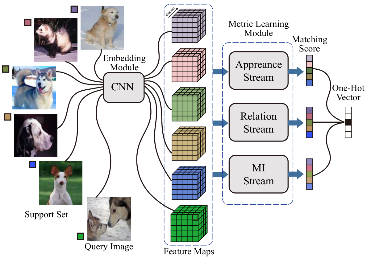
In this paper, we present a novel semantic alignment model for few-shot learning. The framework of our proposed method is illustrated in Figure 1. It mainly consists of three modules: an embedding module, a metric learning module, and a fusion module. The metric learning module is composed of an appearance stream, a relation stream and a mutual information (MI) stream. Among them, the relation stream and the MI stream are introduced for semantic alignment and relation comparing. Given a set of labelled example images and a query image without label, firstly, the images are fed forward into the embedding module, which is a convolutional neural network (CNN) in our paper, for feature extraction. Then the metric learning module compares the deep learned representations of the images to generate a set of matching scores. Finally, through the fusion module, the predicted class label of the query image is obtained by aggregating the matching scores using homoscedastic uncertainty, which can be interpreted as stream-dependent weighting. The propose method can acquire new examples rapidly while providing excellent generalisation from common examples.
Specifically, besides the appearance stream which directly compares the local appearance information between feature pairs, inspired from the spatiotemporal semantic alignment loss [25] introduced to align the feature content from different modalities, we compare query image and example image pairs first by aligning the semantics of the deep representations. We do this by enforcing them to share a common correlation matrix across the deep features of all the samples belonging to the same category. This is done by minimizing the distance between their correlation matrices in the training stage. Since this mechanism can compare the relations of the elements inside an image, we call this a relation stream in our network. In order to take both the positional information and the style information into account, we apply the semantic alignment loss to the correlation matrix across spatial positions as well as the correlation matrix across channels.
Furthermore, we propose to improve the network’s representational capacity by using local-global mutual information, which can solve misalignment and compare relation from another perspective. Maximizing mutual information between input and the learned representations has been widely used in unsupervised representation learning [26, 27]. For few-shot learning, we argue that the mutual information between the images from the same class should be large, while the mutual information between the images from different classes should be small. Given a query image, even if its content is misaligned with that of the example image, a good learning algorithm should be able to conjure up the whole thing through seeing a part of it. Hence, we introduce a MI stream in our network to maximize the mutual information between local patches and the global representation of examples with the same class label. This encourages the embedding module to prefer information that is shared across the same class regardless of locality.
In order to combine the streams optimally and avoid tuning the weights of different streams by hand, which is a difficult and expensive process, we use homoscedastic uncertainty as a basis to weigh losses of different streams automatically.
The main contributions of this paper are summarized as follows:
- •
We introduce a semantic alignment loss to align the content of the features from the same category examples and compare relations among the elements inside an image for few-shot learning.
- •
We propose to maximize local and global mutual information, which allows for representations that contain locally-consistent and class-shared information across structural locations in an image.
- •
Homoscedastic uncertainty is introduced to learn the weights of different streams automatically, which can balance the streams optically and take full advantage of stream combination.
- •
Extensive experiments and analysis demonstrates that the proposed method is capable of comparing relations with semantic alignment strategies, and achieves state-of-the-art performance.
II Related Work
II-A Few-shot learning
Recent years have witnessed a surge of work on the few-shot learning task. We briefly review the three main branches as follows.
Matching network based methods are based on the idea of matching, i.e., the samples belonging to the same category are more similar than the samples belonging to different categories in a feature space. Embedding (mapping the samples to a feature space) and metric learning (measure the similarity) are two key steps. Koch et al. [28] learned image representations with siamese neural network to minimize the distance for similar samples and maximize for distinct ones. Inspired from the ideas of deep neural features based metric learning and external memory augmented neural networks [13], where the metric learning was used to provide good representation for the memory, Vinyals et al. [1] proposed to learn a matching network to map labelled and unlabelled examples to their labels, where the output for a new class was described as a linear combination of the labels in the support set with an attention mechanism. As an extension of matching networks, Prototypical networks [2] learned a metric space in which classification can be performed by computing distances to prototype representations of each class.
For better metric learning ability, Sung et al. [3] added a relation module to compute the relation score between query images and the examples in the support set. Oreshkin et al. [5] employed a task dependent adaptive metric for improved few-shot learning. Instead of pairwise concatenation, Huang et al. [29] utilized pairwise bilinear pooling to extract the second-order features for the pair of query images and support set images. Hao et al. [22] calculated the similarity of each local region pairs of the query image and the support images, and used the similarity to reweight the pairs for comparison. Besides convolutional neural networks and recurrent neural networks, Guo et al. [4] proposed Neural Graph Matching Networks, which jointly learned a graph generator and a graph matching metric function end-to-end.
For better feature learning ability, Li et al. [11] replaced the image-level feature based measure with a local descriptor based measure, which was conducted online via a k-nearest neighbor search over the deep local descriptors. Meanwhile, Lifchitz et al. [12] proposed dense classification over feature maps to take full advantage of the local activations and spatial information. Li et al. [6] introduced a Category Traversal Module to traverse across the entire support set at once, identifying task-relevant features based on both intra-class commonality and inter-class uniqueness in the feature space.
Meta-learner optimization based methods are mainly derived from the idea of learning to learn or meta-learning. The models are learned at two levels, i.e., learning within each task, while accumulating knowledge between tasks. There are two optimizations, the learner, which adapts to new tasks, and the meta-learner, which trains the learner. Santoro et al. [13] proposed a memory-augmented neural network, which was trained to learn how to store and retrieve memories to use for each classification task. There is a series of extensions based on memory-augmented neural network. Shankar et al. [30] organized the memory with the discrete class label as the primary key unlike the previous key being a real vector derived from the input. Mureja et al. [31] explicitly split the external memory into feature and label memories. Ramalho et al. [7] introduced adaptive posterior learning to approximate probability distributions by remembering the most challenging observations it had encountered.
Bertinetto et al. [14] constructed meta-learner and learner as two networks. The meta-learner network is trained to predict the parameters of the learner network. Ravi et al. [15] proposed an LSTM-based meta-learner model to learn both a good initialization and a parameter updating mechanism for the learner network. Finn et al. [16] trained the meta-learner to find an initialization that can be quickly adapted to a new task, via a few gradient steps. Since the initial model of a meta-learner could be too biased towards existing tasks to adapt to new tasks, Jamal et al. [17] proposed an entropy-based approach that meta-learned an unbiased initial model with the largest uncertainty over the output labels. Instead of forcibly sharing an initialization between tasks, Baik et al. [32] employed task-dependent layer-wise attenuation, which could dynamically control how much of prior knowledge each layer would exploit for a given task. Li et al. [8] learned to generate matching networks by learning transferable prior knowledge across tasks and directly producing network parameters for similar unseen tasks.
Data augmentation based methods try to increase the number of training set for better few-shot learning performance. Xian et al. [9] developed a conditional generative model that combined the strength of VAE and GANs, in addition, via an unconditional discriminator, to learn the marginal feature distribution of unlabeled images. Zhang et al. [10] presented two light-weight data hallucination strategies for few-shot learning. Instead of GANs, they leveraged saliency network to obtain foreground-background pairs. Chu et al. [19] proposed a sampling method that decorrrelated an image based on maximum entropy reinforcement learning, and extracted varying sequences of patches on every forward-pass. Self-supervised rotation was used as an auxiliary task in [33] to learn richer visual representations. There are also some methods based on transfer learning [18, 20, 21] where knowledge learned from large enough sample sets are transferred to few samples.
The three branches can be combined in one method. Zhang et al. [34] utilized second-order statistics with power normalization and permutation-based data augmentation to learn the similarity for few-shot learning. Wertheimer et al. [35] proposed batch folding, few-shot localization and covariance pooling for long-tailed class distributions with bounding box annotations. Different from [34, 35], which used second-order statistics rather than first-order statistics to expand feature space, we use the first-order static appearance information, the second-order correlation information, and the local-global mutual information to constrain the model to learn consistent and intrinsic features to address content misalignment for few-shot learning. In our relation stream, we enforce the images belonging to the same class to share a common correlation matrix across spatial positions as well as across channels. Both the relation among spatial local features and the relation among channel style features are taken into account, while other works only considered the first one. We do not use any version of power normalization, bounding box annotations or permutation augmentations in our method. Furthermore, the consistency relationship among features and the multi-stream fusion in our model are optimized with a mutual information stream and uncertainty-based weighting mechanism.
II-B Uncertainty-based learning
Given a model and an input, the uncertainty corresponds to the confidence level of the outcome predicted by the model. In data analysis, it is essential to not only provide a good model but also an uncertainty estimate of the conclusions. It can also be used to improve the robustness and generalization ability of the model. Wang et al. [36] explicitly formulated a propagation uncertainty term to guide the selection of the ambiguous frames for user annotation in video cutout, which reduced manual effort and improved segmentation performance. Khan et al. [37] incorporated both class and sample-level uncertainty estimates to re-adjust the learned boundaries of the classifier for learning unbiased models on imbalanced datasets. Mustafa et al. [38] decreased the uncertainty of the model against attacks by forcing the features of each class to be maximally separated from the polytopes of other classes.
In Bayesian modeling, uncertainty can be categorized into two types one can model: epistemic uncertainty, which accounts for uncertainty in the model parameters, and aleatoric uncertainty, which captures noise inherent in the observations [39]. Aleatoric uncertainty can be further categorized into homoscedastic uncertainty, which stays constant for different inputs, and heteroscedastic uncertainty. Kendall et al. [40] presented a Bayesian deep learning framework combining input-dependent heteroscedastic uncertainty with epistemic uncertainty to improve model’s robustness. For multi-task learning, Kendall et al. [41] utilized homoscedastic uncertainty to weigh losses from different tasks, in order to improve the performance of the model on each task. In our paper, we use homoscedastic uncertainty to automatically aggregate the outputs from multiple streams, avoiding tuning the weights by hand. The tasks of the streams could be different or the same. The final goal is to improve the performance of the output after aggregation. We extend the uncertainty-based weighting strategy from multi-task learning scenario to multi-stream fusion problem, which stimulates its use for automatic weight learning and generalizes its application area.
III Proposed Method
In this section, we give a detailed introduction to the proposed model as shown in Figure 1. Besides an appearance stream, we additionally introduce a relation stream and a mutual information (MI) stream to align content and compare relations. These three streams are complementarily combined, resulting in a model robust to content misalignment.
III-A Network Architecture
There are three major components in the proposed network, the embedding module , the metric learning module and the fusion module. We take a commonly used four-layer convolutional network as the embedding module by default. With the same setting of [3], it contains four convolutional blocks. The first two blocks have an architecture of , where the first digit in parenthesis indicates the kernel size. The last two blocks have an architecture of . This embedding network is named -, since there are 64 filters in each convolutional block. More analysis with a deeper embedding network based on ResNet is shown in the experiment. The metric learning module includes an appearance stream , a relation stream and a mutual information stream , which we will introduce in the following subsections.
For few-shot learning, there is a support set of example images () which contains labeled samples for each class out of classes. It can also be called -way -shot learning. The task is to predict the classes of the images in a query set according to . Episodic training mechanism [13, 1] simulates the few-shot setting to train the network. At each training iteration, sets of , are randomly generated from the entire training set, where denotes the batch size. The images from the support set and the query set are fed forward into the embedding module for feature extraction. Then the metric learning module compares the feature of the query image with the representations corresponding to classes based on the -shot examples to generate a set of matching scores. Finally, the fusion module aggregated these scores to form a global matching score. Each element of the matching score represents the similarity between the query image and the example image among classes, which can predict a probability score for classification. The label is predicted by choosing the category with the maximum probability value.
III-B Appearance Stream


The appearance stream as shown in Figure 2 is retained from the existing few-shot learning work [3]. It replaced non-parametric similarity measure, such as Euclidean distance and cosine similarity, with a network-learned similarity measure. Although it was called RelationNet in the original paper, it focused on comparing local appearance similarity between two images, while discarding the relation among the elements inside an image, which is different from our relation stream. We keep using this stream for appearance information comparison and using the same criteria to measure the pairwise similarities in other streams for convenience and fairness.
Let and denote the feature maps generated by the embedding module with the input of example image and query image respectively. To determine whether and are from matching class or not, the appearance stream predicts a matching score based on the concatenated representation of and . The architecture of is: two convolutional blocks with the same architecture of the first two blocks in , followed by , where the digit in parenthesis indicates the filter numbers.
III-C Relation Stream
In an ideal case, for the samples from the same class, the representations are expected to be consistent and share common semantics. However, in practice, it is hard to learn the high-level complex concept since there is a wide variation and inevitable noise in the samples, especially with only a few examples. In order to learn semantic concepts robust to variation and noises, we propose to use correlation for feature representation and relation comparison. The proposed relation stream is shown in Figure 3. The stream uses multiplicative interactions among local features inside an image to represent the relation information, and measures the image-pairs similarity based on it.
Given , , where , , denote the number of channels, height and width of the feature maps respectively, the feature map can be seen as two feature sets from different aspects. One is the spatial feature set, the other is the channel feature set. Let , () denote the reshaped feature maps. The columns of , are spatial local features. The rows are channel style features. In order to take both the relationship between spatial local features and the relationship between channel style features into account, two correlation matrices are calculated:
| (1) | |||||
| (2) | |||||
| (3) |
where represents the normalization of by subtracting the mean and dividing the standard-deviation of the elements. is the operation to calculate magnitude. Superscript stands for transposition.
Note that the correlation matrix is a Gram matrix that usually used in style transfer tasks [42, 43]. Covariance matrix has also been used to align the source and target feature maps in domain adaptation [44, 45]. We align both the statistics of positional information and the statistics of style information for few-shot learning by predicting matching score based on the distance of the correlation matrices as following:
| (4) | |||||
| (5) |
where represents a fully-connected layer followed by a sigmoid function. The subscripts of and are omitted for clarity.
III-D Mutual Information Stream

Mutual information (MI) describes the association between two variables. Instead of only comparing feature statistics between the support images and the query image, we propose to maximize the mutual information between the images belonging to the same class while minimizing the mutual information between the images from different classes. To learn locally-consistent and class-shared representations across structural locations in the image, we propose to optimize the mutual information between query’s local features and examples’ global description. The proposed local-global MI stream helps the network to learn and compare essential representations regardless of content misalignment and noise. It is complementary to the relation stream. Figure 4 illustrates the structure of MI stream.
For a support set image , its feature map encoded by the embedding module is summarized into a global feature by a global pooling layer. We also have tried other architectures such as using a convolutional sub-network to summarize the feature map. However, experiments show that global max pooling performs superior to average pooling and other architectures. For the query image , its feature map encoded by the embedding module can be seen as a set of spatial local features , index by . We concatenate each with to obtain a new feature map to represent local-global pairs, as shown in Figure 4. The local-global mutual information is estimated with a convolutional sub-network and two fully-connected layers denoted as . We use the estimated local-global mutual information to measure the similarity between two images, i.e., the matching score :
| (6) | |||||
We can also use a dense classifier to estimate the mutual information, i.e., the matching scores on each local-global representation pair separately. Then the dense matching scores are fused to obtain an image-level aggregated matching score.
| (7) | |||||
| (8) |
III-E Full Objective of the Network
Both Mean square error (MSE) and cross-entropy loss (CEL) can be used to train the model. Combining the aforementioned streams, the full objective for training the matching network is as follows:
| (9) |
where , , and are the weights for the loss , , and of different streams, which can be computed as:
where the supervision is 1 for the image pairs belonging to the same class and 0 for mismatched pairs.
III-F Weight Learning with Homoscedastic Uncertainty
Manual tuning the weights of different streams, i.e., , , and , is time-consuming. It is preferable to learn the optimal weights automatically with the training process of the whole network. It was first analyzed in multi-task learning [41] that homoscedastic uncertainty could be used to combine multiple loss functions. We apply the idea of probabilistic modeling to fusing the three streams in our proposed model automatically. Homoscedastic uncertainty is a kind of aleatoric uncertainty which captures noise inherent in the model’s outcome and is independent of the input data. In our multi-stream setting, it varies among different streams, which reflects the relative confidence among streams. It also depends on the measurement scale of each stream. Hence it can be used as a basis for weighting the outcomes in a multi-stream fusion problem. According to the theoretical analysis and formula deduction in [41], the likelihood as a Gaussian of a regression task with MSE loss is:
| (16) | |||||
| (17) | |||||
where represents the ground-truth supervision of a stream, represents the output of the stream with input ( contains feature embedding module and stream-specific part ). is the observation noise scalar.
The likelihood of a classification task with CEL loss can be written as a scaled version:
| (18) | |||
| (19) | |||
where , which often referred to as , is used to scale the input.
We can derive a joint loss of the three streams with homoscedastic uncertainty based on maximizing the log likelihood of the streams:
| (20) | |||||
It should be noted that, regardless of whether the streams correspond to the same task or different tasks, the joint loss can be formulated as above. It applies to our multi-stream fusion objective as shown in Equation 9 and can be seen as learning the relative weights of the losses for each stream. Large decreases the influence of the corresponding stream’s , while small increases its influence. The last three terms are the regularization item, which penalise too large and guarantee that the weights will not converge to zero. Therefore the weights for streams can be optimized automatically with the whole network. For more stable computation, log variance is used to avoid any division by zero. The objective is written as:
| (21) | |||||
i.e., , , and are the learnable weights for the loss , , and of different streams.
IV Experiments
IV-A Datasets
We conduct our experiments on six publicly available few-shot learning datasets with two tasks, i.e., 5-way 1-shot learning and 5-way 5-shot learning.
miniImageNet [1] is a subset of ImageNet [46], which contains 100 classes with 600 images in each class. The spatial resolution of the images is as default setting. Following the same data splits setting of [15], 64, 16 and 20 classes are taken for training, validation and testing respectively. For -way -shot learning, besides the examples for each class, there are 15 and 10 query images for 5-way 1-shot and 5-way 5-shot learning respectively in each training episode. For testing, accuracy averaged over 600 randomly generated episodes is used to measure the performance.
Omniglot [47] consists of 1623 character classes from 50 alphabets. Each class contains 20 samples drawn by 20 people. The spatial resolution of the input images is . 1200 classes are used for training, and the remaining 423 classes are used for testing. We follow the common data augmentation setting and training setting of [3]. For -way -shot learning, besides the examples for each class, there are 19, 15, 10, and 5 query images for 5-way 1-shot, 5-way 5-shot, 20-way 1-shot, and 20-way 5-shot learning respectively in each training episode. When testing, accuracy averaged over 1000 randomly generated episodes is used to measure the performance.
CUB [48] is initially designed for fine-grained classification, which is challenging for few-shot learning since the species are not substantially different from each other. There are 11,788 images of birds over 200 species. Following the commonly used data splitting setting, we randomly sampled 100 species for training, 50 species for validation, and 50 species for testing. We crop the images with the provided bounding box as a pre-processing [49]. The other settings are the same as those on miniImageNet dataset.
tieredImageNet [50] is a larger subset of ImageNet composed of 608 classes rather than 100 for miniImageNet. These classes belong to 34 higher-level categories. To ensure that the training classes are distinct from the testing classes, data splitting is performed at category-level: 20 categories for training, 6 for validation and 8 for testing. The numbers of classes for training, validation and testing are 351, 97 and 160 respectively. The spatial resolution of the input images is 84 84. Following [51], accuracy is averaged over 10,000 sampled tasks for more trustworthy evaluation.
Flower-102 and Food-101 [52, 53] are two other fine-grained datasets like CUB. There are 102 classes of flowers in Flower-102, each containing 40-258 images. And Food-101 is composed of 101 food classes with 1000 images in each class. For both datasets, following [54], we randomly select 80 classes for training and use the remaining classes for testing. The other settings are the same as those on tieredImageNet.
| Setting | |||||||
| only | 1 | 0 | 0 | 0 | 0 | 49.80+-0.82 | |
| only | 0 | 1 | 0 | 0 | 0 | 49.67+-0.83 | |
| only | 0 | 0 | 1 | 0 | 0 | 49.63+-0.81 | |
| only | 0 | 0 | 0 | 1 | 0 | 49.02+-0.86 | |
| only | 0 | 0 | 0 | 0 | 1 | 48.03+-0.86 | |
| manual tuning | 0 | 2 | 1 | 0 | 0 | 51.81+-0.86 | |
| 2 | 1 | 0 | 0 | 0 | 52.00+-0.86 | ||
| 2 | 0 | 1 | 0 | 0 | 51.03+-0.86 | ||
| 4 | 2 | 1 | 0 | 0 | 53.06+-0.88 | ||
| 1 | 0 | 0 | 1 | 0 | 52.22+-0.87 | ||
| 1 | 0 | 0 | 0 | 1 | 52.23+-0.86 | ||
| 1 | 0 | 0 | 1 | 1 | 52.23+-0.87 | ||
| 0 | 2 | 1 | 4 | 0 | 52.67+-0.88 | ||
| 3 streams | 4 | 2 | 1 | 2 | 0 | 53.30+-0.88 | |
| weight learning | ✓ | ✓ | ✓ | 53.03+-0.86 | |||
| ✓ | ✓ | 52.25+-0.87 | |||||
| ✓ | ✓ | ✓ | 52.85+-0.88 | ||||
| ✓ | ✓ | ✓ | ✓ | 53.33+-0.88 | |||
IV-B Implementation Details
By default, the 4-layer convolutional network - is used as the embedding module and the network-learned similarity measure like RelationNet is used. In this case, except for the MI stream, the networks used for miniImageNet, Omniglot, and CUB datasets are the same. To estimate the local-global mutual information, two convolutional blocks with the same architecture of the first two blocks in followed by two fully-connected layers with the same architecture of are used for 8484 input. Since the spatial resolution of Omniglot is small, which is , we remove the last pooling layer for this dataset. All the models are trained end-to-end from scratch with random initialization. Adam is used for optimization. The initial learning rate is and reduced with a fixed decay factor 2 every 100,000 epochs. In our experiments, MSE and CEL have similar performances. We report the results based on MSE as default.
Besides RelationNet with the 4-layer convolutional embedding module, we further demonstrate the usefulness and generalization ability of our method by applying it with different baseline models, e.g., SoSN [34] with the 4-layer embedding module, as well as ProtoNet [2] and RelationNet [3] with a ResNet-12 embedding module. They are based on different similarity measures, e.g., negative Euclidean distance for ProtoNet, and network-learned similarity for RelationNet and SoSN. For the proposed multi-stream model, we keep using the same similarity measure with the baseline model for convenience and fairness. The ResNet-12 embedding module has a same structure with the 12-layer residual network used in [55] and [51]. With a deep embedding module, pre-training on the meta-training set with classification task is suggested and widely used [56, 6, 51]. We use the pre-trained ResNet-12 embedding module of [51] without the last global average pooling layer for parameter initialization. The training and evaluation settings are consistent with the baseline model.
IV-C Ablation Study
IV-C1 Correlation Matrices Comparison
Firstly, we evaluate the performance of the proposed relation stream and add it to the existing appearance matching network [3]. The performance of the appearance stream reported in Table I is reproduced by us with the same setting of [3]. represents the relation stream based on optimizing the similarity of the correlation matrix between spatial local features. And represents the relation stream based on optimizing the similarity of the correlation matrix between channel style features. As we can see, both relation stream and relation stream have a similar performance with the commonly used appearance stream. Note that the relation stream focuses on the relation among the local features inside an image regardless of absolute value and position, which is robust to misalignment and noise. Furthermore, it can be a necessary complement to existing methods. The performance is significantly improved by combing the relation stream and the appearance stream together as shown in Table I. The experimental results demonstrate the effectiveness of the proposed relation stream, indicating that relation is an important factor in few-shot learning and it is complementary to the existing appearance comparison methods.
IV-C2 Mutual Information Optimization


Then we evaluate the performance of the proposed local-global mutual information (MI) stream. The experimental results are also listed in Table I. Simply optimizing the mutual information between the local patches of the query image and the global information of the examples in support set can achieve a performance only slightly lower than that of the appearance comparison method. However it can fundamentally improve the representation learning ability of the network. The MI stream encourages the network to prefer information that is shared across the samples belonging to the same class. It also allows for representations that contain locally-consistent information across structural locations which can deal with misalignment and noise effectively. Experimental results support the above hypothesis since regardless of combining the local-global MI stream with the existing appearance comparison method or with the proposed relation stream, the recognition accuracy can be improved significantly for few-shot learning. Since the two versions of the MI stream play the same role and share a similar performance, we no longer use the dense classifier in the following experiments.
To show that the learned representations are more locally-consistent, we visualize the feature maps of the embedding module trained with and without the MI stream. The input are 3 image samples randomly chosen from the same class and the first 16 channels are shown in Figure 5. We use a sub-network to estimate the local-global MI and set the ground-truth MI for the images belonging to the same class and different classes to be 1 and 0 respectively. The MSE is decreased from 0.4367 to 0.0971 with the MI stream, which supports that applying these local-global pairs can maximize the MI of samples from the same class.
IV-C3 Multi-Stream Fusion
When manual tuning the weights, we evaluate the weights of {1,2,4} for each stream. Taking two streams fusion for example, there are five groups of weights, i.e., {(4:1),(2:1),(1:1),(1:2),(1:4)}. As the number of streams increases, the number of weight combinations grows. We only report the combination with the highest performance in Table I. Since the relation stream and the MI stream are designed to solve misalignment and noise from different perspectives, they are complementary to each other and the appearance stream. As shown in Table I, when the weights of the appearance stream, relation stream , relation stream , and MI stream are , the recognition accuracy for 5-way 1-shot learning on miniImageNet is . The performance is improved by with the proposed relation comparison method. We visualize the matching scores of 15 samples in a batch for the appearance stream and the proposed model in Figure 6.
In order to avoid tuning the weights of different streams by hand, which is a difficult and expensive process, we use homoscedastic uncertainty to weigh losses of different streams automatically. The result is listed in the last block of Table I. With the automatical weight learning method, we only need to train the multi-stream model once, while the performance is comparable or even better than that of manual tuning with multiple times training.
IV-C4 Combination with Different Baseline Models
| Model | Baseline | |||
| RelationNet [3] | 49.80 | 53.03 | 52.25 | 53.33 |
| SoSN [34] () | 52.96 | 54.47 | 54.12 | 54.82 |
| RelationNet (ResNet-12) [3] | 61.51 | 61.97 | 62.39 | 62.68 |
| ProtoNet (ResNet-12) [2] | 62.39 | 62.74 | 63.19 | 63.47 |
Besides the original RelationNet with the 4-layer CNN embedding module, we further apply our method with different baseline models to demonstrate its usefulness and generation ability. The baseline models are SoSN [34] with the 4-layer embedding module, as well as ProtoNet [2] and RelationNet [3] with the ResNet-12 embedding module as introduced in Section IV-B. The experimental results are listed in Table II. Since SoSN already used the second-order correlation across spatial positions which is called in our paper, we add the relation stream with the correlation across channels, i.e., , and the MI stream to it. With the proposed method, the performance is improved by 3.53% and 1.86% for RelationNet and SoSN respectively based on 4-layer embedding module. When using the deep pre-trained ResNet-12 embedding module, we notice that the performance of ProtoNet is superior to that of RelationNet, which is consistent with the conclusion in [57]. Note that there are no extra parameters in the metric learning module when negative Euclidean distance is used like ProtoNet. For the ResNet-12 embedding module, its structure and parameter are designed and pre-trained well for static appearance feature extraction. The extracted feature map has a large number of channels and a low resolution, which increases the difficulty of relation modeling. However, the proposed method still helps a lot for better learning ability. The consistent improvement by combining with our method demonstrates the effectiveness of the proposed method.
| Model | 5-way 1-shot | 5-way 5-shot |
| MatchNet [1] | 46.6% | 60.0% |
| Meta-Learner LSTM [58] | 43.44+-0.77% | 60.60+-0.71% |
| MetaNet [59] | 49.21+-0.96% | - |
| MAML [16] | 48.70+-1.84% | 63.11+-0.92% |
| ProtoNet [2] | 46.14+-0.77% | 65.77+-0.70% |
| ProtoNet# [2] | 49.42+-0.78% | 68.20+-0.66% |
| RelationNet [3] | 50.44+-0.82% | 65.32+-0.70% |
| RelationNet [3] | 49.80+-0.82% | 64.71+-0.69% |
| GNN [60] | 50.33+-0.36% | 66.41+-0.63% |
| CovaMNet [61] | 51.19+-0.76% | 67.65+-0.63% |
| R2D2 [62] | 51.8+-0.2% | 68.4+-0.2% |
| Sampler-FC [19] | 47.18+-0.83% | 66.41+-0.67% |
| Sampler-CS [19] | 51.03+-0.78% | 67.96+-0.71% |
| Localization [35] | 49.64+-0.31% | 69.45+-0.28% |
| SoSN [34] | 52.96+-0.83% | 68.63+-0.68% |
| SoSN+Permutations [34] | 54.72+-0.89% | 68.67+-0.67% |
| DN4 [11] | 51.24+-0.74% | 71.02+-0.64% |
| SAML [22] | 52.22% | 66.49% |
| SAML [22] (224224 input) | 56.68+-0.40% | 71.34+-0.41% |
| FEAT [51] (e=10000) | 55.15+-0.20% | 71.61+-0.16% |
| Ours | 53.33+-0.88% | 68.92+-0.69% |
| Ours (224224 input) | 56.71+-0.90% | 71.50+-0.71% |
| TADAM [5] (ResNet-12) | 58.5% | 76.7% |
| MTL [20] (ResNet-12) | 61.2+-1.8% | 75.5+-0.8% |
| LEO [56] (WRN-28-10, e=50000) | 61.76+-0.08% | 77.59+-0.12% |
| CTM [6] (ResNet-18) | 62.05+-3.84% | 78.63+-4.34% |
| MetaOptNet [55] (ResNet-12) | 62.64+-0.61% | 78.63+-0.46% |
| FEAT [51] (ResNet-12, e=10000) | 66.78+-0.20% | 82.05+-0.14% |
| Ours (ResNet-12, e=10000) | 63.47+-0.20% | 81.27+-0.15% |
| Model | 5-way 1-shot | 5-way 5-shot |
| Masked Soft k-Means [6] | 52.39+-0.44% | 69.88+-0.20% |
| SoSN [34] | 58.62+-0.92% | 75.19+-0.79% |
| CTM [6] (ResNet-18) | 64.78+-3.67% | 81.05+-3.66% |
| MetaOptNet [55] (ResNet-12) | 65.99+-0.72% | 81.56+-0.53% |
| LEO [56] (WRN-28-10, e=50000) | 66.33+-0.05% | 81.44+-0.09% |
| FEAT [51] (ResNet-12, e=10000) | 70.80+-0.23% | 84.79+-0.16% |
| Ours (ResNet-12, e=10000) | 68.58+-0.23% | 84.92+-0.16% |
| Model | 5-way 1-shot | 5-way 5-shot | 20-way 1-shot | 20-way 5-shot |
| MANN [13] | 82.8% | 94.9% | - | |
| Conv-Siamese Net [28] | 97.3% | 98.4% | 88.1% | 97.0% |
| MatchNet [1] | 98.1% | 98.9% | 93.8% | 98.5% |
| Siamese with Memory [63] | 98.4% | 99.6% | 95.0% | 98.6% |
| Neural Statistician [64] | 98.1% | 99.5% | 93.2% | 98.1% |
| MetaNet [59] | 99.0% | - | 97.0% | - |
| ProtoNet [2] | 97.4% | 99.3% | 95.4% | 98.7% |
| ProtoNet# [2] | 98.8% | 99.7% | 96.0% | 98.9% |
| MAML [16] | 98.7+-0.4% | 99.9+-0.1% | 95.8+-0.3% | 98.9+-0.2% |
| RelationNet [3] | 99.6+-0.2% | 99.8+-0.1% | 97.6+-0.2% | 99.1+-0.1% |
| RelationNet [3] | 99.51+-0.20% | 99.75+-0.07% | 97.17+-0.23% | 99.01+-0.08% |
| Sampler-FC [19] | 97.43+-0.28% | 99.51+-0.07% | - | - |
| Sampler-CS [19] | 97.56+-0.31% | 99.65+-0.06% | - | - |
| Two-Stage [65] | 99.2+-0.3% | 99.5+-0.2% | 97.2+-0.3 | 98.9+-0.3 |
| Ours | 99.70+-0.20% | 99.82+-0.09% | 97.49+-0.22% | 99.15+-0.08% |
| Model | 5-way 1-shot | 5-way 5-shot |
| MatchNet* [1] | 60.52+-0.88% | 75.29+-0.75% |
| MAML* [16] | 54.73+-0.97% | 75.75+-0.76% |
| ProtoNet* [2] | 50.46+-0.88% | 76.39+-0.64% |
| mAP-SSVM [49] | 59.0% | - |
| mAP-DLM [49] | 59.1% | - |
| RelationNet* [3] | 62.34+-0.94% | 77.84+-0.68% |
| RelationNet [3] | 61.84+-1.05% | 77.31+-0.72% |
| Baseline [57] | 47.12+-0.74% | 64.16+-0.71% |
| Baseline++ [57] | 60.53+-0.83% | 79.34+-0.61% |
| SAML [22] | 69.33+-0.22% | 81.56+-0.15% |
| FEAT [51] (e=10000) | 68.87+-0.22% | 82.90+-0.15% |
| Ours (e=10000) | 69.57+-0.25% | 81.73+-0.16% |
| Model | Flower-102 | Food-101 | ||
| 1-shot | 5-shot | 1-shot | 5-shot | |
| ProtoNet [2] | 62.81% | 82.11% | 36.71% | 53.43% |
| RelationNet [3] | 68.52% | 81.11% | 36.89% | 49.07% |
| SoSN [34] | 76.27% | 88.55% | 43.12% | 58.13% |
| MsSoSN (3 scales) [54] | 81.65% | 92.10% | 50.87% | 66.32% |
| MsSoSN+SS+SD+DD [54] | 84.69% | 94.21% | 53.86% | 68.67% |
| Ours (ResNet-12) | 84.92% | 94.52% | 56.21% | 73.94% |
IV-D Comparison with State-of-the-Art
We compare our method with the state-of-the-art approaches on miniImageNet, tieredImageNet, Omniglot, CUB, Flower-102 and Food-101 datasets with several learning settings. Although our method can be combined with multiple state-of-the-art models, without loss of generality, we use RelationNet based on shallow embedding module and ProtoNet based on deep embedding module for comparison.
IV-D1 Results on miniImageNet and tieredImageNet datasets
The results on the miniImageNet dataset are shown in Table III. Among the methods based on 4-layer convolutional embedding modules, our proposed method outperforms most of the other methods significantly. The comparison with some representative methods are analyzed in detail as follows.
Localization [35] and SoSN [34] also used second-order statistics for few-shot learning. However, the Localization model [35] localized objects using bounding box annotations before classification and computed the cross-covariance between the predicted foreground and background maps, which helped a lot in performance improvement. SoSN made a thorough analysis in second-order statistics and power normalization functions. The derived sigmoid-like power normalizing function can improve the performance of 5-way 1-shot and 5-shot learning on miniImageNet from 50.88% and 66.71% to 52.96% and 68.63%, which demonstrates its effectiveness and provides insight for the society. They also proposed to permute the second-order matrices to capture various correlations with multiple similarity networks, which can be seen as data augmentation. We propose to learn and compare appearance and relation features separately and complementarily to solve content misalignment for few-shot learning. We use the first-order static appearance information, the second-order correlation information, and the local-global mutual information to constrain the model to learn consistent and intrinsic features. The learning procedure can be regarded as optimization with multiple constraints. In our relation stream, we enforce the features of the same category to share a common correlation matrix. Both the relation among spatial local features and the relation among channel style features are taken into account, while other works only considered the first one. It should be noted that there is only 1 fully-connected layer to estimate the matching score based on the difference of the correlation matrices. And we do not use any version of extra annotations, power normalizations or permutation based augmentations in our method.
DN4 [11] and SAML [22] are based on local descriptors for similarity computation. DN4 conducted online k-nearest neighbor search over the deep local descriptors. Under the 1-shot setting, our proposed method achieves 53.33% accuracy, which is more than 2% higher than that of DN4. Under the 5-shot setting, DN4 performs better. The performance of DN4 depends heavily on the number of samples and the value of k. As the number of shots increases, the number of local descriptors to be compared increases, hence its performance gets better and better. However, the computational complexity also increases. Different from DN4 searching from the entire support set, we assemble the shots to serve as prototypes for each class like ProtoNet, which reduces complexity while lost some information. SAML calculated the similarity of each local region pairs and used attention to aggregate the pairs’ similarities for image comparison. Besides the input, they also reported the recognition accuracy with input. Our method outperforms SAML in all the settings. Simply using input instead of input, the performance of our method can yields up to 3% improvement, yielding the highest accuracies for both 1-shot and 5-shot learning except FEAT [51].
Instead of using the same embedding function for all tasks, FEAT [51] proposed to adapt the embedding to each target few-shot learning task with a Transformer based set-to-set function, which improves the performance significantly. They also used a more trustworthy evaluation setting with 10,000 sampled tasks instead of 600 sampled tasks. We follow to use this evaluation in the experiments based on the deep embedding module. As shown in the lower part of Table III, among the methods based on deep embedding modules, our proposed method outperforms all the other methods except FEAT. The result on the tieredImageNet dataset is consistent with that on the miniImageNet dataset as shown in Table IV. Our method even surpasses FEAT under 5-way 5-shot setting on the tieredImageNet. CTM [6] and MetOptNet [55] also shared the same spirit of learning task-specific features, whose performances are inferior to mine. As analyzed above, the deep embedding module is designed and pre-trained well for appearance feature extraction, hence the accuracy is boosted drastically compared to shallow models. However, the extracted feature map with the deep embedding module has a large number of channels and a low resolution, which increases the difficulty of relation modeling. In the future we will explore more about the structure of relation modeling and combination with embedding adaptation methods to further promote the performance.
IV-D2 Results on Omniglot and CUB datasets
We compare our method with other representative methods on the Omniglot dataset and CUB dataset, whose results are listed in Table V and Table VI respectively. It should be noted that, on the CUB dataset, the performance of our method is on par with FEAT under 5-way 5-shot setting, and even better than FEAT by 0.7% under 1-shot setting. The experimental results demonstrate the effectiveness of our method, especially for fine-grained dataset. The proposed method not only pays more attention to the relation information inside images, which is insensitive to the absolute value, but it can also encourage the network to learn locally-consistent essential features shared among images from the same class. As a result, it allows for high representation quality and a generic system robust to content misalignment and noise.
IV-D3 Results on Flower-102 and Food-101 datasets
To further support the conclusion, we evaluate our method on another two fine-grained datasets, i.e., Flower-102 and Food-101. The results are listed in Table VII. MsSoSN [54] is a multi-scale version of SoSN, which not only used input, but also used and inputs. MsSoSN+SS+SD+DD represent adding a scale selector, a scale discriminator, and a discrepancy discriminator to MsSoSN in addition. Instead of using multi-scale inputs, we report the performance of our method based on the ResNet-12 embedding module and input. Our method achieves a new state-of-the-art performance on these datasets.
V Conclusion
In order to address content misalignment for few-shot learning, we propose a novel semantic alignment model with multiple streams to compare relations as well as for better representation and metric learning ability. We introduce a relation stream to align and compare correlation relations among the elements inside an image. To take both the relationship of positional features and the relationship of style features into account, we apply constraint to the correlation matrix across spatial positions as well as the correlation matrix across channels. Besides that, the local-to-global consistency relation is optimized with a mutual information stream. This stream plays an important role in the quality of the representation learning. Locally-consistent and intra-class shared features are encouraged. The two proposed streams not only perform well by themselves but also can be fused with the existing appearance comparison methods mutual reinforcingly with learnable weights, demonstrating the effectiveness of our proposed method and indicating that semantic relation robust to misalignment is an important factor in few-shot learning.
References
- [1] O. Vinyals, C. Blundell, T. Lillicrap, D. Wierstra et al., “Matching networks for one shot learning,” in Advances in neural information processing systems, 2016, pp. 3630–3638.
- [2] J. Snell, K. Swersky, and R. Zemel, “Prototypical networks for few-shot learning,” in Advances in Neural Information Processing Systems, 2017, pp. 4077–4087.
- [3] F. Sung, Y. Yang, L. Zhang, T. Xiang, P. H. Torr, and T. M. Hospedales, “Learning to compare: Relation network for few-shot learning,” in Proceedings of the IEEE Conference on Computer Vision and Pattern Recognition, 2018, pp. 1199–1208.
- [4] M. Guo, E. Chou, D.-A. Huang, S. Song, S. Yeung, and L. Fei-Fei, “Neural graph matching networks for fewshot 3d action recognition,” in Proceedings of the European Conference on Computer Vision, 2018, pp. 653–669.
- [5] B. Oreshkin, P. R. López, and A. Lacoste, “Tadam: Task dependent adaptive metric for improved few-shot learning,” in Advances in Neural Information Processing Systems, 2018, pp. 721–731.
- [6] H. Li, D. Eigen, S. Dodge, M. Zeiler, and X. Wang, “Finding task-relevant features for few-shot learning by category traversal,” in Proceedings of the IEEE Conference on Computer Vision and Pattern Recognition, 2019, pp. 1–10.
- [7] T. Ramalho and M. Garnelo, “Adaptive posterior learning: few-shot learning with a surprise-based memory module,” arXiv preprint arXiv:1902.02527, 2019.
- [8] H. Li, W. Dong, X. Mei, C. Ma, F. Huang, and B.-G. Hu, “Lgm-net: Learning to generate matching networks for few-shot learning,” in International conference on machine learning, 2019, pp. 3825–3834.
- [9] Y. Xian, S. Sharma, B. Schiele, and Z. Akata, “f-vaegan-d2: A feature generating framework for any-shot learning,” in Proceedings of the IEEE Conference on Computer Vision and Pattern Recognition, 2019, pp. 10 275–10 284.
- [10] H. Zhang, J. Zhang, and P. Koniusz, “Few-shot learning via saliency-guided hallucination of samples,” in Proceedings of the IEEE Conference on Computer Vision and Pattern Recognition, 2019, pp. 2770–2779.
- [11] W. Li, L. Wang, J. Xu, J. Huo, Y. Gao, and J. Luo, “Revisiting local descriptor based image-to-class measure for few-shot learning,” in Proceedings of the IEEE Conference on Computer Vision and Pattern Recognition, 2019, pp. 7260–7268.
- [12] Y. Lifchitz, Y. Avrithis, S. Picard, and A. Bursuc, “Dense classification and implanting for few-shot learning,” in Proceedings of the IEEE Conference on Computer Vision and Pattern Recognition, 2019, pp. 9258–9267.
- [13] A. Santoro, S. Bartunov, M. Botvinick, D. Wierstra, and T. Lillicrap, “Meta-learning with memory-augmented neural networks,” in International conference on machine learning, 2016, pp. 1842–1850.
- [14] L. Bertinetto, J. F. Henriques, J. Valmadre, P. Torr, and A. Vedaldi, “Learning feed-forward one-shot learners,” in Advances in Neural Information Processing Systems, 2016, pp. 523–531.
- [15] S. Ravi and H. Larochelle, “Optimization as a model for few-shot learning,” in International Conference on Learning Representations, 2017.
- [16] C. Finn, P. Abbeel, and S. Levine, “Model-agnostic meta-learning for fast adaptation of deep networks,” in Proceedings of the 34th International Conference on Machine Learning-Volume 70. JMLR. org, 2017, pp. 1126–1135.
- [17] M. A. Jamal and G.-J. Qi, “Task agnostic meta-learning for few-shot learning,” in Proceedings of the IEEE Conference on Computer Vision and Pattern Recognition, 2019, pp. 11 719–11 727.
- [18] Y.-X. Wang and M. Hebert, “Learning to learn: Model regression networks for easy small sample learning,” in Proceedings of the European Conference on Computer Vision. Springer, 2016, pp. 616–634.
- [19] W.-H. Chu, Y.-J. Li, J.-C. Chang, and Y.-C. F. Wang, “Spot and learn: A maximum-entropy patch sampler for few-shot image classification,” in Proceedings of the IEEE Conference on Computer Vision and Pattern Recognition, 2019, pp. 6251–6260.
- [20] Q. Sun, Y. Liu, T.-S. Chua, and B. Schiele, “Meta-transfer learning for few-shot learning,” in Proceedings of the IEEE Conference on Computer Vision and Pattern Recognition, 2019, pp. 403–412.
- [21] A. Li, T. Luo, Z. Lu, T. Xiang, and L. Wang, “Large-scale few-shot learning: Knowledge transfer with class hierarchy,” in Proceedings of the IEEE Conference on Computer Vision and Pattern Recognition, 2019, pp. 7212–7220.
- [22] F. Hao, F. He, J. Cheng, L. Wang, J. Cao, and D. Tao, “Collect and select: Semantic alignment metric learning for few-shot learning,” in Proceedings of the IEEE International Conference on Computer Vision, 2019, pp. 8460–8469.
- [23] T.-Y. Lin, A. RoyChowdhury, and S. Maji, “Bilinear cnn models for fine-grained visual recognition,” in Proceedings of the IEEE international conference on computer vision, 2015, pp. 1449–1457.
- [24] L. Wang, W. Li, W. Li, and L. V. Gool, “Appearance-and-relation networks for video classification,” in Proceedings of the IEEE Conference on Computer Vision and Pattern Recognition, 2018, pp. 1430–1439.
- [25] M. Abavisani, H. R. V. Joze, and V. M. Patel, “Improving the performance of unimodal dynamic hand-gesture recognition with multimodal training,” in Proceedings of the IEEE Conference on Computer Vision and Pattern Recognition, 2019, pp. 1165–1174.
- [26] R. D. Hjelm, A. Fedorov, S. Lavoie-Marchildon, K. Grewal, P. Bachman, A. Trischler, and Y. Bengio, “Learning deep representations by mutual information estimation and maximization,” in International Conference on Learning Representations, 2019.
- [27] C. Sun, F. Baradel, K. Murphy, and C. Schmid, “Contrastive bidirectional transformer for temporal representation learning,” arXiv preprint arXiv:1906.05743, 2019.
- [28] G. Koch, R. Zemel, and R. Salakhutdinov, “Siamese neural networks for one-shot image recognition,” in ICML deep learning workshop, vol. 2, 2015.
- [29] H. Huang, J. Zhang, J. Zhang, Q. Wu, and J. Xu, “Compare more nuanced: Pairwise alignment bilinear network for few-shot fine-grained learning,” arXiv preprint arXiv:1904.03580, 2019.
- [30] S. Shankar and S. Sarawagi, “Label organized memory augmented neural network.” arXiv preprint arXiv:1707.01461, 2017.
- [31] D. Mureja, H. Park, and C. D. Yoo, “Meta-learning via feature-label memory network,” arXiv preprint arXiv:1710.07110, 2017.
- [32] S. Baik, S. Hong, and K. M. Lee, “Learning to forget for meta-learning,” arXiv preprint arXiv:1906.05895, 2019.
- [33] S. Gidaris, A. Bursuc, N. Komodakis, P. Pérez, and M. Cord, “Boosting few-shot visual learning with self-supervision,” in Proceedings of the IEEE International Conference on Computer Vision, 2019, pp. 8059–8068.
- [34] H. Zhang and P. Koniusz, “Power normalizing second-order similarity network for few-shot learning,” in 2019 IEEE Winter Conference on Applications of Computer Vision (WACV). IEEE, 2019, pp. 1185–1193.
- [35] D. Wertheimer and B. Hariharan, “Few-shot learning with localization in realistic settings,” in Proceedings of the IEEE Conference on Computer Vision and Pattern Recognition, 2019, pp. 6558–6567.
- [36] W. Wang, J. Shen, and F. Porikli, “Selective video object cutout,” IEEE Transactions on Image Processing, vol. 26, no. 12, pp. 5645–5655, 2017.
- [37] S. Khan, M. Hayat, S. W. Zamir, J. Shen, and L. Shao, “Striking the right balance with uncertainty,” in Proceedings of the IEEE/CVF Conference on Computer Vision and Pattern Recognition, 2019, pp. 103–112.
- [38] A. Mustafa, S. H. Khan, M. Hayat, R. Goecke, J. Shen, and L. Shao, “Deeply supervised discriminative learning for adversarial defense,” IEEE transactions on pattern analysis and machine intelligence, 2020.
- [39] A. Der Kiureghian and O. Ditlevsen, “Aleatory or epistemic? does it matter?” Structural safety, vol. 31, no. 2, pp. 105–112, 2009.
- [40] A. Kendall and Y. Gal, “What uncertainties do we need in bayesian deep learning for computer vision?” in Conference on Neural Information Processing Systems, 2017, pp. 5574–5584.
- [41] A. Kendall, Y. Gal, and R. Cipolla, “Multi-task learning using uncertainty to weigh losses for scene geometry and semantics,” in Proceedings of the IEEE conference on computer vision and pattern recognition, 2018, pp. 7482–7491.
- [42] L. A. Gatys, A. S. Ecker, and M. Bethge, “Texture synthesis using convolutional neural networks,” in Advances in Neural Information Processing Systems, 2015, pp. 262–270.
- [43] L. A. Gatys, A. S. Ecker, and M. Bethge, “Image style transfer using convolutional neural networks,” in Proceedings of the IEEE Conference on Computer Vision and Pattern Recognition, 2016, pp. 2414–2423.
- [44] B. Sun and K. Saenko, “Deep CORAL: correlation alignment for deep domain adaptation,” in Proceedings of the European Conference on Computer Vision Workshops, 2016, pp. 443–450.
- [45] P. Morerio, J. Cavazza, and V. Murino, “Minimal-entropy correlation alignment for unsupervised deep domain adaptation,” in International Conference on Learning Representations, 2018.
- [46] O. Russakovsky, J. Deng, H. Su, J. Krause, S. Satheesh, S. Ma, Z. Huang, A. Karpathy, A. Khosla, M. Bernstein et al., “Imagenet large scale visual recognition challenge,” International journal of computer vision, vol. 115, no. 3, pp. 211–252, 2015.
- [47] B. Lake, R. Salakhutdinov, J. Gross, and J. Tenenbaum, “One shot learning of simple visual concepts,” in Proceedings of the annual meeting of the cognitive science society, vol. 33, no. 33, 2011.
- [48] C. Wah, S. Branson, P. Welinder, P. Perona, and S. Belongie, “The caltech-ucsd birds-200-2011 dataset,” 2011.
- [49] E. Triantafillou, R. Zemel, and R. Urtasun, “Few-shot learning through an information retrieval lens,” in Advances in Neural Information Processing Systems, 2017, pp. 2255–2265.
- [50] M. Ren, E. Triantafillou, S. Ravi, J. Snell, K. Swersky, J. B. Tenenbaum, H. Larochelle, and R. S. Zemel, “Meta-learning for semi-supervised few-shot classification,” in International Conference on Learning Representations. OpenReview.net, 2018.
- [51] H.-J. Ye, H. Hu, D.-C. Zhan, and F. Sha, “Few-shot learning via embedding adaptation with set-to-set functions,” in Proceedings of the IEEE/CVF Conference on Computer Vision and Pattern Recognition, 2020, pp. 8808–8817.
- [52] M.-E. Nilsback and A. Zisserman, “Automated flower classification over a large number of classes,” in 2008 Sixth Indian Conference on Computer Vision, Graphics & Image Processing. IEEE, 2008, pp. 722–729.
- [53] L. Bossard, M. Guillaumin, and L. Van Gool, “Food-101–mining discriminative components with random forests,” in European conference on computer vision. Springer, 2014, pp. 446–461.
- [54] H. Zhang, P. H. Torr, and P. Koniusz, “Few-shot learning with multi-scale self-supervision,” arXiv preprint arXiv:2001.01600, 2020.
- [55] K. Lee, S. Maji, A. Ravichandran, and S. Soatto, “Meta-learning with differentiable convex optimization,” in Proceedings of the IEEE/CVF Conference on Computer Vision and Pattern Recognition, 2019, pp. 10 657–10 665.
- [56] A. A. Rusu, D. Rao, J. Sygnowski, O. Vinyals, R. Pascanu, S. Osindero, and R. Hadsell, “Meta-learning with latent embedding optimization,” in International Conference on Learning Representations. OpenReview.net, 2019.
- [57] W. Chen, Y. Liu, Z. Kira, Y. F. Wang, and J. Huang, “A closer look at few-shot classification,” in International Conference on Learning Representations, 2019.
- [58] S. Ravi and H. Larochelle, “Optimization as a model for few-shot learning,” in International Conference on Learning Representations, 2017.
- [59] T. Munkhdalai and H. Yu, “Meta networks,” in Proceedings of the 34th International Conference on Machine Learning-Volume 70. JMLR. org, 2017, pp. 2554–2563.
- [60] V. G. Satorras and J. B. Estrach, “Few-shot learning with graph neural networks,” in International Conference on Learning Representations, 2018.
- [61] W. Li, J. Xu, J. Huo, L. Wang, Y. Gao, and J. Luo, “Distribution consistency based covariance metric networks for few-shot learning,” in Proceedings of the AAAI Conference on Artificial Intelligence, vol. 33, 2019, pp. 8642–8649.
- [62] L. Bertinetto, J. F. Henriques, P. H. S. Torr, and A. Vedaldi, “Meta-learning with differentiable closed-form solvers,” in International Conference on Learning Representations, 2019.
- [63] L. Kaiser, O. Nachum, A. Roy, and S. Bengio, “Learning to remember rare events,” in International Conference on Learning Representations, 2017.
- [64] H. Edwards and A. J. Storkey, “Towards a neural statistician,” in International Conference on Learning Representations, 2017.
- [65] D. Das and C. G. Lee, “A two-stage approach to few-shot learning for image recognition,” IEEE Transactions on Image Processing, 2019.