Decentralized Multi-player Multi-armed Bandits
with No Collision Information
Chengshuai Shi Wei Xiong Cong Shen Jing Yang
University of Virginia University of Virginia University of Virginia Pennsylvania State University
Abstract
The decentralized stochastic multi-player multi-armed bandit (MP-MAB) problem, where the collision information is not available to the players, is studied in this paper. Building on the seminal work of Boursier and Perchet, 2019, we propose error correction synchronization involving communication (EC-SIC), whose regret is shown to approach that of the centralized stochastic MP-MAB with collision information. By recognizing that the communication phase without collision information corresponds to the Z-channel model in information theory, the proposed EC-SIC algorithm applies optimal error correction coding for the communication of reward statistics. A fixed message length, as opposed to the logarithmically growing one in Boursier and Perchet, 2019, also plays a crucial role in controlling the communication loss. Experiments with practical Z-channel codes, such as repetition code, flip code and modified Hamming code, demonstrate the superiority of EC-SIC in both synthetic and real-world datasets.
1 Introduction
| Model | Reference | Asymptotic Upper Bound (up to constant factor) |
|---|---|---|
| Centralized Multiplayer | Komiyama et al., 2015 | |
| Decentralized, Col. Sensing | SIC-MMAB (Boursier and Perchet, 2019) | |
| Decentralized, No Sensing | Lugosi and Mehrabian, 2018 | |
| Decentralized, No Sensing | Lugosi and Mehrabian, 2018 | |
| Decentralized, No Sensing | ADAPTED SIC-MMAB (Boursier and Perchet, 2019) | |
| Decentralized, No Sensing | SIC-MMAB2 (Boursier and Perchet, 2019) | |
| Decentralized, No Sensing | EC-SIC (this paper) |
: number of arms; : number of players; is -th order statistics of ; ; ; is the random coding error exponent.
Recent years have witnessed an increased interest in the multi-player multi-armed bandits (MP-MAB) problem, in which multiple players simultaneously play the bandit game and interact with each other through arm collisions. In particular, motivated by the practical application of cognitive radio (Anandkumar et al., 2011), decentralized stochastic MP-MAB problems have been widely studied. See Section 7 for a review of the related work.
Since the stochastic MAB problem for a single player is well understood, a predominant approach in decentralized MP-MAB is to let each player play the single-player MAB game while avoiding collisions for as much as possible (Liu and Zhao, 2010; Avner and Mannor, 2014; Rosenski et al., 2016; Besson and Kaufmann, 2018). Intuitively, this would allow the algorithm to behave as the single-player MAB. Comparing to the centralized MP-MAB, there is a multiplicative factor (number of players) increase in the regret coefficient of . This has long been considered fundamental due to the lack of communication among players.
Recently, a surprising and inspiring approach, called SIC-MMAB, is proposed in Boursier and Perchet, 2019 for the collision-sensing MP-MAB problem. Instead of viewing collision as detrimental, Boursier and Perchet, 2019 purposely instigates collisions as a way to communicate between players. With a careful design, an internal rank can be assigned to each player and arm statistics can be completely shared among players at a communication cost that does not dominate the arm exploration regret, which leads to an overall regret approaching the centralized setting. The proposed communication phase transmits the total reward by using collision/no-collision to represent bit 1/0. The theoretical analysis shows, for the first time, that the regret of a decentralized MP-MAB algorithm can approach that of the centralized counterpart, which represents a significant progress in decentralized MP-MAB.
The no-sensing problem, on the other hand, represents arguably the most difficult setting in MP-MAB and there has been little progress in the literature. Boursier and Perchet, 2019 makes two attempts to generalize the forced collision idea to this setting. Directly applying SIC-MMAB to this setting leads to a O() regret, which has an additional multiplicative coefficient due to no sensing. In other words, a straightforward application of SIC-MMAB results in the communication loss dominating the total regret. Then, the authors propose a different approach: use communication only to exchange the accepted and rejected arms, thus reducing the regret caused by communication. However, this approach, philosophically speaking, deviates from the core idea of SIC-MMAB and does not fully utilize the communication benefit of collision (arm statistics are not shared among players). This is also the reason why the multiplicative factor reappears in the regret formula, which was eliminated in the collision-sensing case by SIC-MMAB. It remains an open problem whether a decentralized MP-MAB algorithm without collision information can approach the performance of its centralized counterpart.
In this work, we return to the original idea of utilizing collisions to communicate sampled arm rewards. By modelling no collision information as the Z-channel communication problem in information theory, we propose to incorporate optimal error correction coding in the communication phase to control the error rate of decoding the message. With this approach, we are able to transmit a quantized sample reward mean with a fixed length for each player without having the communication loss dominate the total regret. The resulting asymptotic regret improves the coefficients over SIC-MMAB2, and represents the best known regret in the no-sensing MP-MAB model to the best of the authors’ knowledge. Table 1 compares the asymptotic regret upper bounds for different algorithms. We also propose two practical enhancements that significantly improve the algorithm’s empirical performance. Numerical experiments on both synthetic and real-world datasets corroborate the analysis and offer interesting insights into EC-SIC.
2 The No-Sensing MP-MAB Problem
In the standard (single player) stochastic MAB setting, there are arms, with rewards of arm sampled independently from a distribution on , where . At time , a player chooses an arm and the goal is to receive the highest mean cumulative reward in rounds.
In this section, we introduce the no-sensing multiplayer MAB model with a known number of arms but an unknown number of players . The horizon is known to the players. At each time step , all the players simultaneously pull the arms and receive the reward such that
where is the collision indicator defined by with .
If players can observe both and , it is the collision-sensing problem. On the other hand, in the no-sensing case as in our paper, players can only access , i.e., a reward of can indistinguishably come from a collision with another player or . Note that if , the no-sensing and collision-sensing models are equivalent11 1 We further note that the no-sensing model can be generalized to an arbitrary but bounded reward support where collision results in the lowest value in the support..
The performance in the standard single-player MAB setting is usually measured by the regret:
where is the expected reward of the arm with the highest expected reward. As shown in the lower bound by Lai and Robbins, 1985, the optimal order of the regret cannot be better than .
In the multiplayer setting, the notion of regret can be generalized and defined with respect to the best allocation of players to arms, as follows:
where is -th order statistics of , i.e. .
Two technical assumptions are made in this paper, which are also widely used in the literature. The first is a strictly positive lower bound of , which has been used by Lugosi and Mehrabian, 2018 and Boursier and Perchet, 2019 for the no-sensing model. The second assumption is a finite gap between the optimal and suboptimal (group of) arms; see Avner and Mannor, 2014; Kalathil et al., 2014; Rosenski et al., 2016; Nayyar et al., 2016.
Assumption 1.
- 1)
A positive lower bound of is known to all players: .
- 2)
There exists a positive gap , and it is known to all players.
Assumption 1.1 is equivalent to , . This also bounds . Note that although provides a lower bound for , Assumption 1.1 does not require the exact value of . The gap in Assumption 1.2 measures the difficulty of the bandit game and ensures the existence of only one optimal choice.
3 The EC-SIC Algorithm
The proposed error correction synchronization involving communication (EC-SIC) is compactly described in Algorithm 1. Similar to SIC-MMAB, the overall algorithm can be structurally divided into four phases: initialization phase, exploration phase, communication phase, and exploitation phase. It is important to note that all players are synchronized in running EC-SIC, i.e., they enter each phase at the same time (or at least with high probability in some cases) except the exploitation phase. Until a player fixates on a specific arm and enters the exploitation phase, the algorithm keeps iterating between the exploration and communication phases. Players that have (not) entered the exploitation phase are called inactive (active). We denote the set of active players during the -th phase by and its cardinality by . Similarly, arms that have not been decided to be optimal or sub-optimal are called active. The set of active arms during the -th phase is denoted by with cardinality .
3.1 Initialization phase
The same structure of the initialization phase as Boursier and Perchet, 2019 is used in EC-SIC, which outputs an internal rank for each player as well as the estimated value of . It starts with a “Musical Chair” phase and is followed by a so-called Sequential Hopping protocol. The full procedure is described in Appendix B.1 for completeness.
3.2 Exploration phase
During the -th exploration phase, active players sequentially hop among the active arms for steps, and any active arm is pulled times by each active player. Since the hopping is based on each player’s internal rank, the exploration phase is collision-free.
We note that the length of an exploration phase is different from Boursier and Perchet, 2019, which is a key component of the performance improvement. The difference of a factor, in fact, results in an overall rounds of exploration and communication phases in the ADAPTED SIC-MMAB algorithm of Boursier and Perchet, 2019. This directly leads to a dominating communication loss that breaks the order-optimality. With an expansion of length by in EC-SIC, the overall rounds become a constant, and the communication regret can be better controlled as shown in Section 4.
3.3 Communication phase
In the communication phase, all players attempt to exchange their sampled reward information in a synchronized and distributed manner. The communication takes place via a careful collision design. All players enter this phase synchronously and, by default, keep pulling different arms based on their internal ranks. Then, when it is player ’s turn to communicate with player , she would purposely pull (not pull) player ’s arm as a way to communicate bit 1 (0). If player can fully access the collision information, i.e., knowing whether collision happens or not at each time step, she will be able to receive the bit sequence successfully, which conveys player ’s sample reward statistics. However, for the no-sensing model, such error-free communication becomes impossible.
Three new ideas are used in the communication phase of EC-SIC. The first is the introduction of Z-channel coding. In the no-sensing scenario, players cannot directly identify collision. If the same communication protocol in Boursier and Perchet, 2019 (representing or by collision or no collision) is used, the confusion may mislead the player to believe that collision has occurred (bit ) while it is actually a null statistic of reward sampling (bit ). This error has a catastrophic consequence in that it breaks the essential synchronization between players. We are thus facing the challenge of communicating the reward statistics to other users while controlling the error rate for the overall communication loss to not dominate the regret.

Luckily, this is the well-known reliable communication over a noisy channel problem, one of the foundations in information theory. In particular, our communication channel is asymmetric: (collision) is always received correctly and (no collision) may be received incorrectly with a certain probability . This corresponds to the Z-channel model (see Fig.1) in information theory (Tallini et al., 2002), which represents a broad class of asymmetric channels. The Z-channel has a crossover probability of that corresponds to 22 2 Since the crossover probability is unknown and varies for different arm , is used to capture the worst case..
The Z-channel capacity is derived in Tallini et al., 2002 as follows.
Theorem 1.
The capacity of a Z-channel with crossover probability is:
| (1) |
Shannon theory guarantees that as long as the coding rate is below in Eqn. (1), there exists at least one code that allows for an arbitrarily low error rate asymptotically. This means that theoretically, for this Z-channel, it is possible to transmit information nearly error-free when the rate is close to bits per channel use. In reality, however, different finite block-length channel codes may have different performances; we thus evaluate several practical codes both theoretically (in Section 4) and experimentally (in Section 6). For simplicity, Functions Send(), Receive(), Encoder() and Decoder() are used in the algorithm as the sending and receiving protocol and the encoder and corresponding decoder, respectively.
The second enhancement is to transmit each arm’s quantized sample reward mean with a fixed length. The reason not to use the total reward as Boursier and Perchet, 2019 is that the gradually increasing total reward leads to a message length , which cannot be transmitted efficiently in the no-sensing case with bits. However, with a finite gap, a less precise statistics sharing is tolerable as long as it does not affect the choice of optimal arms. For a quantized sample mean of length , the error is at most . We thus control the length such that , where is a pre-defined constant. By constructing as the confidence bound, analysis in Section 4 shows that acceptation and rejection maintain a high probability of success.
Lastly, compared to the mesh-structured communication in Boursier and Perchet, 2019, it is more efficient to form a tree structure that one player (“leader”) gathers all statistics and makes decisions for others (“followers”). The player with internal rank becomes the leader and the rest become the followers (Kaufmann and Mehrabian, 2019). Statistics of arms are transmitted from followers to the leader. The leader decides the set of arms to be accepted or rejected by comparing their upper confidence bounds and lower confidence bounds with each other, and sends back to the followers. Upon reception, active players either enter another iteration of exploration and communication, or begin exploitation. This process utilizes reward statistics from all players and has better communication efficiency. Procedures for the leader and followers are given in Algorithm 2 and 3, respectively.
4 Theoretical Analysis
The overall regret of EC-SIC can be decomposed as . The first, second and third term refers to the regret caused by the initialization, exploration, and communication phase, respectively. The main result is presented in Theorem 2, and each component regret is subsequently analyzed. Detailed proofs can be found in Appendix B.
Theorem 2.
With an optimal coding technique that achieves Gallager’s error exponent for the corresponding Z-channel with crossover probability , for any , we have
| (2) | ||||
where , and are constants and .
Theorem 2 involves an information-theoretic concept called error exponent, which is explained in Theorem 3 in Section 4.2 but more details can be found in (Gallager, 1968).
An asymptotic upper bound can be obtained from (2) with :
|
|
(3) |
Compared to SIC-MMAB2, we have successfully removed the multiplicative factor of in the first term. This is due to the efficient communication phase that transmits the reward statistics. In addition, we have a factor in the second term, as opposed to in SIC-MMAB2. This is also an improvement since . We also note that Eqn. (2) and Eqn. (3) hold when is replaced by .
To prove Theorem 2, we first define the “typical event” as the success of initialization, communication and exploration throughout the entire horizon . More specifically, we define three events: each player has a correct estimation of and an orthogonal internal rank after initialization; messages are decoded correctly in all communication phases; . We use to denote the probability that the typical event happens, which is . The regret caused by the “atypical event” can be simply bounded by a linear regret . Then the result of (2) can be proved by controlling to balance both events.
4.1 Initialization phase
Similar to Lemma 11 in Boursier and Perchet, 2019, we can bound the regret of initialization as follows.
Lemma 1.
With probability , event happens. Furthermore, the regret of the initialization phase satisfies:
4.2 Exploration phase
The regret due to exploration is bounded in Lemma 2.
Lemma 2.
With probability , the typical event happens and the exploration regret conditioned on the typical event satisfies:
|
|
We first present a fundamental result of channel coding for communication in a noisy channel, known as the error exponent (Gallager, 1968).
Theorem 3.
For a discrete memoryless channel, if , there exists a code of block length without feedback such that the error probability is bounded by
where is the random coding error exponent with rate .
We note that the error exponent used in Theorem 2 corresponds to .
Theorem 3 suggests that, to transmit a -bit message over a Z-channel, there exists an optimal coding scheme with length to achieve an error rate less than , where . Several of the existing coding techniques, although not optimal, can achieve this error rate with , which only leads to a multiplicative factor larger than but does not change the regret order. For example, with repetition code, flip code and modified Hamming code, we have , , respectively (see Appendix A for detailed analysis of practical codes). The remaining analysis will be based on the optimal channel coding with the caveat that a “good” Z-channel code should be applied in practice.
With at most exploration and communication phases and arms to be accepted or rejected, there are at most communication instances on arm statistics, communication instances on the number of acc/rej arms, and communication instances on the index of acc/rej arms. A simple union bound analysis leads to the following result.
Lemma 3.
Denoting the probability that event holds by , with an optimal Z-channel code of , we have
Lemma 3 guarantees all communications are correct. To bound the probability that all arms are correctly estimated, we have the following result.
Lemma 4.
In phase , for any active arm ,
With at most exploration-communication phases, event happens with probability:
| (4) |
A union bound argument leveraging , and leads to probability for the typical event to happen, as defined in Lemma 2. Finally, for the exploration phases, the number of times that an arm is pulled before being accepted or rejected are well controlled.
Lemma 5.
In the typical event, every optimal arm is accepted after at most pulls, and every sub-optimal arm is rejected after at most pulls.
Denote as the overall time of exploration and exploitation phase and as the number of time steps where the -th best arm is pulled during these two phases. With no collision in exploration and exploitation, the exploration regret can be decomposed as (Anantharam et al., 1987)
| (5) | ||||
Both components in (5) can be upper bounded by Lemma 7 in Appendix B.2.4, which proves Lemma 2.
4.3 Communication phase
Thanks to the expanded length of each exploration phase and the fixed-length quantization of arm statistics, the regret does not dominate the overall regret, as stated in Lemma 6.
Lemma 6.
In the typical event,
|
|
We note that becomes a constant when is sufficiently large. Noting that , the communication loss has the same order as other phases.
4.4 Overall regret
When the typical event happens, the overall regret is bounded by the sum of and ; otherwise, for the atypical event, the regret can be upper bounded as . Thus, the overall regret satisfies




5 Algorithm Enhancement
EC-SIC has nice theoretical performance guarantees, but we have noticed that in practice some minor enhancements improve its performance significantly, which are shown in the next section. First, after each exploration and communication phase, player can use the active arm with the -th best empirical mean (sent by the leader) as her communication arm for the next around, instead of the -th active arm. Since players keep receiving rewards from their communication arms while waiting for communication or receiving bit , using an arm with higher empirical mean can lead to a lower loss in these time steps.
Second, we have observed in practice that the first one or two explorations do not lead to effective acceptation or rejection even when the game is easy, which means all the communication losses during these phases are incurred with no benefit (this is much larger than the exploration loss). Thus, can be initialized to a larger integer (e.g. ), which leads to a longer exploration to start with and less ineffective communication.
6 Experiments
Numerical experiments have been carried out to verify the analysis of EC-SIC and compare its empirical performance to other methods. All rewards follow the Bernoulli distributions with , and we set . Results are obtained by averaging over 500 experiments. More detailed discussions and additional results can be found in Appendix C.
We compare state of the art algorithms under both easy and difficult bandit game settings. EC-SIC (with repetition code), ADAPTED SIC-MMAB, SIC-MMAB2, and the algorithm proposed by Lugosi and Mehrabian, 2018 (labeled as “no-sensing-MC”) are first compared in a relatively easy game (). Fig. 7 shows that even in an easy game, no-sensing-MC could not finish exploration within time steps, and ADAPTED SIC-MMAB has poor performance compared to the other two. Both EC-SIC and SIC-MMAB2 converge to the optimal arm set quickly, but the overall regret of EC-SIC is smaller. For a hard game with , Fig. 7 shows that EC-SIC is superior to SIC-MMAB2.
A detailed comparison of EC-SIC with SIC-MMAB2 is done by comparing their regrets as a function of the gap in Fig.7. We see that when the game is not extremely difficult (), EC-SIC has better performance since players benefit from sharing statistics. When becomes extremely small, the required communication length increases significantly, leading to a dominating communication regret in EC-SIC that cannot be offset by the benefits of sharing statistics.
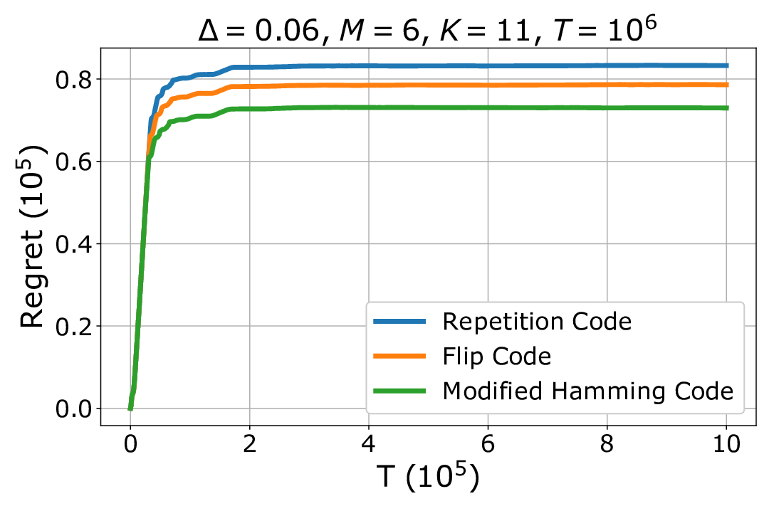
Fig. 7 reports the performance while using different Z-channel codes in communication. We observe that modified Hamming Code has the best performance, which is due to its superior error correction capability. This observation also implies that with a near-optimal code that is specifically designed for Z-channel, performance of EC-SIC can be further improved.
We also evaluate the impact of codeword length on the regret. For our simulation setting, the theoretical analysis requires a repetition code length to transmit one bit, in order to achieve an error rate of . We are interested in evaluating whether the theoretically required code length can be shortened in practice. Under the easy game setting of Fig. 7 with rounds averaging, Fig. 7 shows that with decreasing from to , the regret decreases . More importantly, it shows that the convergence of EC-SIC does not change. When further reducing to , we see the regret curve trends upward at large , which represents a non-negligible loss due to unsuccessful communications. With , the regret increases rapidly, indicating that players suffer from an increased error rate. It is thus essential to strike a balance between error rate and communication loss.
Lastly, we evaluate EC-SIC on a real world dataset: the movie watching dataset (ml-20m) from MovieLens (Harper and Konstan, 2015). It consists of watching data of more than movies from over users between January 09, 1995 and March 31, 2015. In the pre-processing, we group these movies into categories by their total number of views from high to low. The binary reward at time (hour) is defined as whether there are users watching films in this group, and we replicate it to a final reward sequence of length . players are assumed to engage in the game. This final sequence has and . Compared to synthetic datasets, this setting poses a larger and more difficult game. For each experiment, the reward sequence is randomly shuffled. We report the cumulative regret of EC-SIC and SIC-MMAB2, averaged over experiments, in Figure 7. One can see that the advantage of EC-SIC over SIC-MMAB2 is significant for this real-world dataset. Intuitively, this is because the game is hard ()33 3 However, the game is also not too hard for communication to be ineffective as the case of Fig. 7., and and are also large.
7 Related Work
Depending on how information is shared and actions are determined, existing literature can be categorized into centralized or decentralized (distributed) MP-MAB problems. The centralized scenario can be viewed as an application of the multiple-play bandit (Anantharam et al., 1987; Komiyama et al., 2015). A more interesting and challenging problem, introduced by Liu and Zhao, 2010 and Anandkumar et al., 2011, lies in the decentralized scenario where explicit communications between players are not allowed and thus collision may happen. For the collision-sensing MP-MAB problem, earlier works attempt to let each player play the single-player MAB game while avoiding collisions for as much as possible; see (Liu and Zhao, 2010; Avner and Mannor, 2014; Rosenski et al., 2016) for some representative approaches.
The SIC-MMAB algorithm in Boursier and Perchet, 2019 is closely relevant to our work, which proposes to exploit collisions as opposed to avoiding them. Proutiere and Wang, 2019 further refines this idea and decreases the communication regret so that the lower bound of the centralized setting can be approached asymptotically for Bernoulli distributed rewards. The SIC-MMAB principle has subsequently been applied to other multi-player settings. For example, Kalathil et al., 2014 considers an extended multiplayer model where reward distribution varies for each player. Bistritz and Leshem, 2018 proposes a Game of Thrones algorithm that achieves a regret of . This is further improved by Kaufmann and Mehrabian, 2019, leading to an improved regret of .
The no-sensing model, on the other hand, is very challenging and limited progress has been made so far. In Lugosi and Mehrabian, 2018, sample means are rectified by the probability of collision and then the same Musical Chair approach is adopted. As discussed in Section 1, Boursier and Perchet, 2019 touches upon the no-sensing model with ADAPTED SIC-MMAB and SIC-MMAB2. However, the former has a communication loss of that dominates the total regret, while the latter drifts away from communication of full statistics, thus is fundamentally incapable of approaching the centralized performance.
8 Conclusion
In this work, we have proposed the EC-SIC algorithm for the no-sensing MP-MAB problem with forced collision. We proved that it is possible for a decentralized MP-MAB algorithm without collision information to approach the performance of its centralized counterpart. Recognizing that communication under the no-sensing setting corresponds to the Z-channel model in information theory, optimal error correction codes are applied for reliable communication via collision. With this tool, we return to the original idea of utilizing forced collisions to share complete arm statistics among players. By expanding exploration phases and fixing the message length, an order-optimal communication loss is achieved. Practical simulation results with several Z-channel codes have proved the superiority of EC-SIC algorithm under different bandit game settings, using both synthetic and real-world datasets.
Acknowledgements
JY acknowledges the support from U.S. National Science Foundation under Grant ECCS-1650299.
References
- Anandkumar et al., (2011) Anandkumar, A., Michael, N., Tang, A. K., and Swami, A. (2011). Distributed algorithms for learning and cognitive medium access with logarithmic regret. IEEE Journal on Selected Areas in Communications, 29(4):731–745.
- Anantharam et al., (1987) Anantharam, V., Varaiya, P., and Walrand, J. (1987). Asymptotically efficient allocation rules for the multiarmed bandit problem with multiple plays - part I: IID rewards. IEEE Trans. Autom. Control, 32(11):968–976.
- Avner and Mannor, (2014) Avner, O. and Mannor, S. (2014). Concurrent bandits and cognitive radio networks. In Joint European Conference on Machine Learning and Knowledge Discovery in Databases, pages 66–81. Springer.
- Barbero et al., (2006) Barbero, A., Ellingsen, P., Spinsante, S., and Ytrehus, O. (2006). Maximum likelihood decoding of codes on the Z-channel. In IEEE International Conference on Communications, volume 3, pages 1200–1205. IEEE.
- Besson and Kaufmann, (2018) Besson, L. and Kaufmann, E. (2018). Multi-player bandits revisited. In Proceedings of Algorithmic Learning Theory, pages 56–92.
- Bistritz and Leshem, (2018) Bistritz, I. and Leshem, A. (2018). Distributed multi-player bandits - a game of thrones approach. In Advances in Neural Information Processing Systems, pages 7222–7232.
- Boursier and Perchet, (2019) Boursier, E. and Perchet, V. (2019). SIC-MMAB: Synchronisation involves communication in multiplayer multi-armed bandits. In Advances in Neural Information Processing Systems, pages 12071–12080.
- Chen et al., (2013) Chen, P.-N., Lin, H.-Y., and Moser, S. M. (2013). Optimal ultrasmall block-codes for binary discrete memoryless channels. IEEE Transactions on Information Theory, 59(11):7346–7378.
- Gallager, (1968) Gallager, R. G. (1968). Information theory and reliable communication. John Wiley & Sons, USA.
- Harper and Konstan, (2015) Harper, F. M. and Konstan, J. A. (2015). The MovieLens datasets: History and context. ACM Transactions on Interactive Intelligent Systems, 5(4).
- Kalathil et al., (2014) Kalathil, D., Nayyar, N., and Jain, R. (2014). Decentralized learning for multiplayer multiarmed bandits. IEEE Transactions on Information Theory, 60(4):2331–2345.
- Kaufmann and Mehrabian, (2019) Kaufmann, E. and Mehrabian, A. (2019). New algorithms for multiplayer bandits when arm means vary among players. arXiv preprint arXiv:1902.01239.
- Komiyama et al., (2015) Komiyama, J., Honda, J., and Nakagawa, H. (2015). Optimal regret analysis of Thompson sampling in stochastic multi-armed bandit problem with multiple plays. In Proceedings of the 32nd International Conference on Machine Learning, pages 1152–1161, Lille, France.
- Lai and Robbins, (1985) Lai, T. L. and Robbins, H. (1985). Asymptotically efficient adaptive allocation rules. Advances in applied mathematics, 6(1):4–22.
- Liu and Zhao, (2010) Liu, K. and Zhao, Q. (2010). Distributed learning in multi-armed bandit with multiple players. IEEE Transactions on Signal Processing, 58(11):5667–5681.
- Lugosi and Mehrabian, (2018) Lugosi, G. and Mehrabian, A. (2018). Multiplayer bandits without observing collision information. arXiv preprint arXiv:1808.08416.
- Nayyar et al., (2016) Nayyar, N., Kalathil, D., and Jain, R. (2016). On regret-optimal learning in decentralized multiplayer multiarmed bandits. IEEE Transactions on Control of Network Systems, 5(1):597–606.
- Proutiere and Wang, (2019) Proutiere, A. and Wang, P.-A. (2019). An optimal algorithm in multiplayer multi-armed bandits. arXiv preprint arXiv:1909.13079.
- Rosenski et al., (2016) Rosenski, J., Shamir, O., and Szlak, L. (2016). Multi-player bandits – a musical chairs approach. In Proceedings of The 33rd International Conference on Machine Learning, pages 155–163.
- Tallini et al., (2002) Tallini, L. G., Al-Bassam, S., and Bose, B. (2002). On the capacity and codes for the Z-channel. In Proceedings of the IEEE International Symposium on Information Theory, page 422.
Supplementary Material: Decentralized Multi-player Multi-armed Bandits with No Collision Information
Chengshuai Shi Wei Xiong Cong Shen Jing Yang
University of Virginia University of Virginia University of Virginia Pennsylvania State University
Appendix A Error Correction Codes for Communication over the Z-channel
More details about the representative coding techniques for the Z-channel are provided in this section.
A.1 Repetition code
Repetition code seems simple but is surprisingly powerful in the Z-channel. Chen et al., 2013 has proved that it is the optimal code for . The encoding and decoding processes are described as follows.
- •
Encoding. Repeat bit or bit in message for times to generate codeword .
- •
Decoding. For channel output , if there exists such that , then the decoder outputs 0. Otherwise, we have for all , and the decoder outputs 1.
With a crossover probability no larger than , the bit error probability is:
For a message length of bits, the error probability is:
With the choice of , we have . Thus, the total code length for a -bit message is:
With , the regret remains order-optimal.
A.2 Flip code
The flip code is designed by Chen et al., 2013 to better utilize the Z-channel property. The encoding and decoding processes are illustrated with the case of 4 codewords as follows.
- •
Encoding. Assuming we encode every two bits into a -bit codeword, the encoding function is:
- •
Decoding. It is similar to the repetition code. A codeword of length will be divided into of length and of length
- –
if all bits in and are s, decoder outputs ;
- –
if all bits in are s and contains , decoder outputs ;
- –
if contains and all bits in are s, decoder outputs ;
- –
for all other cases, decoder outputs .
- –
With a crossover probability no larger than , the bit error probability is (Chen et al., 2013):
The inequality holds because the function monotonically increases for . For a message length of bits (we assume is even here, otherwise an additional bit can always be padded to make it even), the error probability is:
With the choice of , we have . Thus, the total codeword length for a message of length is:
With , the regret remains order-optimal.
A.3 Modified Hamming code
As the number of codewords increases to (4 bits), a modified (,) Hamming Code can be designed. It is a concatenated code, with the standard (,) Hamming code as the inner code and a repetition code as the outer code.
- •
Encoding. The standard (7,4) Hamming encoding matrix is first used to encode a 4-bit message to a 7-bit codeword. Then we repeat each bit of the 7-bit codeword times, leading to a -bit codeword;
- •
Decoding. First by using the repetition code’s decoding rule, -bit coded message is decoded into bits. This bits is then decoded with the standard (7,4) Hamming decoding matrix . The final output is a decoded -bit message.
The repetition code reduces the crossover probability from to . With this relatively small crossover probability and the error correction capability of the Hamming Code, a reliable performance can be achieved. As stated by Barbero et al., 2006, with as the crossover probability, we have the following error rate for the Hamming Code over a Z-channel.
We neglect in the following analysis. The error probability of transmitting -bit messages (assuming can be divided by ) using the (,) modified Hamming code is:
| (6) | ||||
By choosing , we have . Thus, the total codeword length for a message of length is:
which is still , but the bound in (6) indicates an improvement over the repetition code and flip code.
Appendix B Proofs for the Regret Analysis
B.1 Initialization phase
The initialization phase starts with a “Muscial Chair” phase, which assigns a unique external rank in for each of the player. Then the following sequential hopping protocol converts the external rank into a unique internal rank in for each player and estimates the number of players . The proof for Lemma 1 is the same as Lemma 11 in Boursier and Perchet, 2019. We re-state the algorithm and the proof for the sake of completeness.
Proof.
As there is at least one arm that is not played by all the other players, the probability to encounter a positive reward for player during the Musical Chair process at time is lower bounded by . Thus with the choice of , the probability for a single player to encounter only zero rewards until time is:
Applying a union bound over all players, the Musical Chair process is successful with a probability at least .
Now we analyze the Estimate_M_NoSensing protocol. Similar to using repetition code for communication, the probability that a player detects a “collision” while there is none is:
The union bound over the players and the blocks yields that it will be successful with a probability at least . Furthermore, the initialization phase lasts time steps. Hence the regret satisfies:
∎
B.2 Exploration phase
This section aims at proving Lemma 2, which bounds the exploration regret. We start with the required lemmas and then go back to proving Lemma 2.
B.2.1 Proof for Lemma 3
This lemma ensures that event happens with a high probability. As mentioned before, there are at most communication phases, which leads to at most instances of transmissions to send arm statistics to the leader and send the acc/rej arm sets to the followers. Since there are at most arms to be accepted or rejected, no more than instances of transmissions are required for sending the acc/rej arm sets.
Proof.
Denote as the probability that the decoding of a -bit message produces a wrong result at round . With the choice of , and , denoting the message before encoding and after decoding at round , we have
A simple union bound leads to
∎
B.2.2 Proof for Lemma 4
Lemma 4 ensures the acceptance and rejection of arms are successful with a high probability, which requires a good estimation of the statistics of arms. The estimation error consists of two parts: the quantization error and the sampling error. We analyze them separately.
Proof.
With the choice of , the quantization error in phase can be bounded as:
For any active arm , the gap between the sample mean (using all players’ samples) and the true mean can be bounded with Hoeffding’s inequality:
Then, the overall gap between the quantized mean and the true mean for any active arm can be bounded as:
There are at most iterations of exploration and communication. By using a union bound of all these iterations and arms, Eqn. (4) is obtained. ∎
B.2.3 Proof for Lemma 5
Lemma 5 bounds the number of time steps an arm is pulled before being accepted or rejected, and is essential to control the rounds of exploration and communication. The proof is similar to the proof to Proposition 1 in Boursier and Perchet, 2019.
Proof.
The proof is conditioned on the typical event. We first consider an optimal arm . Let be the gap between the arm and the first sub-optimal arm. Let be the first integer such that . It satisfies:
Recall that the number of time steps an active arm is pulled before the -th exploration is . With a non-increasing , it holds that
| (7) |
For some such that , the following inequalities are in order: ; ; and for all sub-optimal arm . We then have
This suggests arm will be accepted at time . Eqn. (7) also leads to . Thus, arm will be accepted after at most pulls. The part of rejecting sub-optimal arms can be similarly proved with . ∎
B.2.4 Lemma 7 and its proof
Lemma 7.
In the typical event, the following results hold.
The proof of the first part in Lemma 7 is as follows.
Proof.
For a sub-optimal arm , Lemma 5 leads to , and thus
in which inequality (i) comes from
and . Inequality (ii) can be obtained with the observation that the term is maximized by . ∎
Lemma 8.
Define as the number of exploratory pulls before accepting/rejecting the arm and is the total number of exploration phases. Conditioned on the typical event, we have:
Proof.
For an optimal arm , during phase , if has already been accepted, it will be pulled times. If it is still active (i.e., ), it will be pulled times, meaning that this arm is not pulled for times. Thus, it holds that . Notice that . We have , which proves the lemma. ∎
Lemma 9.
Conditioned on the typical event, we have:
Proof.
Define . Notice that
and denote . The inequity implies . We also denote as the smallest integer satisfying . Then we have the following:
Since , . Thus,
With the definition of , we have . With inequality we have . then holds. With , we have
∎
B.3 Communication phase
This section presents the proof related to the bound of the communication regret.
B.3.1 Proof for Lemma 6
Proof.
Conditioned on the typical event, we denote as the number of exploration phases. The communication length for sending arm statistics and acc/rej arm sets for is at most . Lemma 5 states that satisfies . Thus,
which leads to a regret of . Next, transmitting acc/rej arm sets at most incurs a regret of . Putting them together, the total communication regret is:
∎
Appendix C Supplementary Materials for Experiments
C.1 Minor changes to SIC-MMAB2
Some minor changes can be made to SIC-MMAB2 (Boursier and Perchet, 2019) to improve its convergence and make it more practical. First, the original length of exploration in phase is , where . The factor is too large and makes it almost impossible to converge (or even finish one round of exploration) in the time horizon of our experiments. We thus change it to , and we have verified that it converges successfully for the instances in the experiments. Another minor change is to add a random selection in the declaration phases. In SIC-MMAB2 (Boursier and Perchet, 2019), players sequentially declare the arms in their own rejected sets. However, with similar exploration time steps across players, the declaration sets are almost identical for all players. With a sequential selection (rather than a random selection in our implementation), all players will declare the same arm with high probability, which is in fact noticed to happen very frequently in the experiment.
C.2 Supplementary experiment results


The impact of the leader-follower protocol and the enhancement in Section 5 are evaluated in a larger game (, ). With , EC-SIC without the leader-follower protocol (labeled as “EC-SIC-Mesh”), EC-SIC using none of the enhancement in Section 5 (labeled as “EC-SIC-NE”) are compared with EC-SIC and SIC-MMAB2. Compared to the stable performance of EC-SIC and SIC-MMAB2, Fig. 9 shows that in practice, due to the unnecessary communication between every pair of players, EC-SIC-Mesh cannot even finish the first communication phase. Although it converges eventually, EC-SIC-NE has a larger regret. These results highlight the benefit of the tree-structured communication and the selection of better communication arms.
In the case of utilizing repetition code in EC-SIC, we carry on experiments to evaluate the dependency on the knowledge of . For , we evaluate EC-SIC and SIC-MMAB2 with from to , hence creating a mismatched “estimation” of . The results shown in Figure 9 state that decreasing leads to an increasing regret of both SIC-MMAB2 and EC-SIC, which corroborates the theoretical analysis. Furthermore, EC-SIC has better performance than SIC-MMAB2 across different “estimates” of .
The knowledge of is assumed in the algorithms and their theoretical analysis. In practice, a precise value of may not always be available. In the last experiment, we demonstrate the robustness of the algorithms by feeding it with inaccurate information instead of the true . As shown in Figure 11, with a pessimistic estimation of , the inaccurate information only leads to some additional but acceptable communication loss. The overall regret is still better than SIC-MMAB2. For the optimistic estimations, Figure 11 shows that the algorithm is effective even with . When the estimation error further grows ( or ), communication errors start to occur, which lead to a few arms that are identified incorrectly. It nevertheless still outperforms SIC-MMAB2 in terms of regret. Thus, practically speaking, EC-SIC has good robustness, and we further comment that it is preferable to have a pessimistic estimation.

