Noncommutative generalized Gibbs ensemble in isolated integrable quantum systems

The foundation of quantum statistical mechanics has seen a resurgence of interest in recent years D’Alessio et al. 2016; Eisert et al. 2015; Ilievski et al. 2016; Mori et al. 2018 partly because well-isolated and -controlled artificial quantum systems have emerged as the ideal platform to reconsider the long-standing problem Kinoshita et al. 2006; Trotzky et al. 2011; Langen et al. 2013; Langen et al. 2015; Schreiber et al. 2015; Kaufman et al. 2016. A remarkable finding is that an isolated quantum many-body system can relax to an effective stationary state even without energy dissipation or quantum decoherence. Although the stationary state in the strict sense appears only in infinite systems, an effective (or approximate) stationary state arises at large but finite system sizes, where the fluctuations and recurrences are negligible Tasaki 1998; Reimann 2008; Linden et al. 2009.

In generic nonintegrable systems, the effective stationary state coincides in fact with the thermal state due to the eigenstate thermalization hypothesis (ETH) Deutsch 1991; Srednicki 1994, which dates back to von Neumann von Neumann 2010 and has recently been numerically verified Rigol et al. 2008; Santos and Rigol 2010; Kim et al. 2014; Beugeling et al. 2014; Steinigeweg et al. 2014; Khodja et al. 2015; Yoshizawa et al. 2018. Meanwhile, there exist known systems in which the stationary state does not coincide with the thermal state such as integrable systems Rigol et al. 2007; Santos and Rigol 2010; Biroli et al. 2010; Ikeda et al. 2013; Alba 2015, many-body localized systems Pal and Huse 2010; Iyer et al. 2013, and so on van den Worm et al. 2013; Shiraishi and Mori 2017; Mondaini et al. 2018. It remains an open question how to classify all the nonthermal systems and to identify the statistical-mechanical ensemble describing those states.

The generalized Gibbs ensemble (GGE) is a paradigmatic framework to describe various nonthermal stationary states Rigol et al. 2007. Whereas the usual Gibbs (canonical) ensemble involves the Hamiltonian, the GGE does other conserved quantities as well (see Eq. (5) below) Jaynes 1957. The GGE describes the stationary states in noninteracting integrable models (hard-core bosons Rigol et al. 2007, the transverse-field Ising model Vidmar and Rigol 2016), interacting (Bethe-ansatz) integrable ones Caux and Konik 2012; Pozsgay 2013; Fagotti et al. 2014; Wouters et al. 2014; Pozsgay et al. 2014; Wouters et al. 2014; Ilievski et al. 2015, models with different-type conserved quantities Hamazaki et al. 2016, quantum field theories Cardy 2016, and so on Kollar and Eckstein 2008; Kollar et al. 2011.

Despite its success, the GGE sometimes fails to describe the stationary state. For example, Spinless fermions or hard-core bosons under incommensurate potential cannot be described by the GGE due to the localization of single particle eigenstate Caneva et al. 2011; He et al. 2013; Ziraldo et al. 2012; Ziraldo and Santoro 2013; Wang and Tong 2017. Another example is the entanglement prethermalization in an interacting integrable system Kaminishi et al. 2015, where nonlocal conserved quantities play significant roles. One crucial problem is that the GGE is a general framework and never tells us which conserved quantities should be incorporated. When a GGE fails, it is hard to tell whether the ad hoc set of conserved quantities is not enough or the framework breaks down. In particular, the GGEs mentioned above implicitly assume that the conserved quantities commute with each other (commutative GGE, CGGE), and this assumption may unnecessarily constrain the GGE. the GGE conserved quantities can be noncommutative in view of the maximum entropy principle. The GGE with a noncommutative set of conserved quantities was first introduced in Ref. Fagotti 2014 in discussing the prerelaxation for the XY spin chain. The ensemble with a noncommutative set of conserved quantities was also mentioned in Ref. Yukalov 2011. However, it has not been systematically studied why and how those GGEs describe local or few-body observables well.

In this paper, we systematically study how the additional noncommutative conserved quantities affect the GGE and show that the GGE thus generalized (noncommutative GGE, NCGGE) describes the stationary states in isolated integrable systems better than the conventional CGGE. By introducing the observable projection idea, we provide a clear understanding of why the (NC)GGE well describes the stationary states. In this spirit, for a noninteracting model, we systematically construct the NCGGE that describes the stationary states without an error at finite system size for few-body observables. We also propose some extensions of the NCGGE and demonstrate how they work.

The rest of this paper is organized as follows. In Sec. II, we formulate the problem and define the NCGGE. In Sec. III, we explain why the GGE is valid with enough conserved quantities and the necessity of the NCGGE. The observable projection idea and the uniqueness of the NCGGE presented in Secs. II and III are so general that they can be applied to both interacting and noninteracting integrable systems. In Secs. IV and V, focusing on free fermions, we show more detailed analyses of the NCGGE. In Sec. IV, we give the example of NCGGE in free fermion and show the exactness of NCGGE even at finite system size. In Sec. V, we give numerical results for two-body observables in the CGGE and NCGGE. In Sec. VI, we give further extensions of the NCGGE. Finally, in Sec. VII, we summarize our study with concluding remarks.

We consider an isolated quantum system described by a time-independent Hamiltonian $\hat{H}$. We let $\{E_{n}\}$ denote the distinct eigenenergies, having $\hat{H}=\sum_{m}E_{m}\hat{P}_{m}$ with $\hat{P}_{m}$ being the projection operator onto the corresponding eigenspace. Under the Hamiltonian, an initial state $\ket{\psi_{\text{ini}}}$ evolves as $\ket{\psi(t)}=e^{-iHt}\ket{\psi_{\text{ini}}}=\sum_{m}e^{-iE_{m}t}\hat{P}_{m}\ket{\psi_{\text{ini}}}$ at time $t$ ($\hbar=1$ throughout this paper). Assuming that $\ket{\psi_{\text{ini}}}$ is a superposition of exponentially-large number (in terms of the system size) of energy eigenstates Reimann 2008; Short 2011; Reimann and Kastner 2012, we have an effective stationary state, in which an observable $\hat{A}$ has its expectation value equal to the long-time average

where $\overline{f(t)}\equiv\lim_{T\rightarrow\infty}\int_{0}^{T}(dt/T)f(t)$. It is convenient to define the diagonal and off-diagonal decomposition of $\hat{A}$ by $\hat{A}=\hat{\overline{A}}+\delta\hat{A}$ with $\hat{\overline{A}}\equiv\sum_{m}\hat{P}_{m}\hat{A}\hat{P}_{m}$ and $\delta\hat{A}\equiv\sum_{m,n\,(m\neq{n})}\hat{P}_{m}\hat{A}\hat{P}_{n}$. This notation simplifies Eq. (1) as

If $\hat{A}$ is a conserved quantity $\hat{Q}$, i.e. $[\hat{Q},\hat{H}]=0$, Eq. (1) leads to

Equation (1) gives $\braket{\hat{A}}_{\mathrm{LT}}$ exactly but involves an exponentially-large number of inputs corresponding to every detail of $\ket{\psi_{\text{ini}}}$. The question that we address in this paper is to find a statistical-mechanical ensemble $\rho$ which, with fewer (up to a polynomially-large number of) inputs, satisfies $\braket{\hat{A}}_{\mathrm{LT}}\simeq\text{Tr}(\hat{\rho}\hat{A})$ for local or few-body observables $\hat{A}$’s of interest. Here, $\simeq$ allows an error due to the finite-size effect that vanishes in the thermodynamic limit.

The GGE is a successful candidate for such an ensemble formulated as follows. The central idea is that the ensemble $\hat{\rho}$ would maximize the von Neumann entropy $S(\rho)=-\text{Tr}(\hat{\rho}\log\hat{\rho})$ (the Boltzmann constant is set to unity). When there exist multiple conserved quantities $\{\hat{Q}_{\alpha}\}$ including the Hamiltonian, the dynamics is constrained by Eq. (3) for each $\hat{Q}=\hat{Q}_{\alpha}$. Then the ensemble that maximizes the entropy under the constraints is given by the stationary condition for

with the generalized temperatures $\{\lambda_{\alpha}\}$. This condition leads to Jaynes 1957

where $Z\equiv\text{Tr}\,e^{-\sum_{\alpha}\lambda_{\alpha}\hat{Q}_{\alpha}}$ is the partition function and the Lagrange multipliers $\{\lambda_{m}\}$ called the generalized temperatures are determined uniquely by

for each $\alpha$. When $\{\hat{Q}_{\alpha}\}$ consists only of the Hamiltonian, the GGE reduces to the usual Gibbs (canonical) ensemble and the generalized temperature is the inverse temperature $\beta$. Once determined, the GGE gives expectation values for generic observables by $\braket{\hat{A}}_{\text{GGE}}\equiv\text{Tr}(\hat{\rho}_{\mathrm{GGE}}\hat{A})$.

We emphasize that, in deriving Eq. (5), we never use the commutativity $[\hat{Q}_{\alpha},\hat{Q}_{\beta}]=0$, which is implicitly assumed in the literature. In the Heisenberg model, for example, the SU(2) symmetry implies that each of the total $S^{x}$, $S^{y}$, and $S^{z}$ is a conserved quantity, and one can construct the GGE by using all of them. Thus, allowing noncommutative ones increases the number of conserved quantities and improves the GGE in general.

We note that, when $[\hat{Q}_{\alpha},\hat{Q}_{\beta}]\neq 0$, we cannot decompose Eq. (5) into the exponentials for each conserved quantity: $e^{-\sum_{\alpha}\lambda_{\alpha}\hat{Q}_{\alpha}}\neq\prod_{\alpha}e^{-\lambda_{\alpha}\hat{Q}_{\alpha}}$. Nevertheless, the exponential $e^{-\sum_{\alpha}\lambda_{\alpha}\hat{Q}_{\alpha}}$ is well-defined and the generalized temperatures are uniquely determined. We prove these facts in the Appendix A.

Before discussing concrete models, we show why the GGE well describes the long-time behaviors (1) for generic observables in the thermodynamic limit. Although the GGE is usually justified by the generalized ETH Cassidy et al. 2011, we here provide another perspective, in which the merit of the NCGGE becomes evident.

To justify the GGE, we invoke the observable projection with conserved quantities Mierzejewski and Vidmar 2020. Note that the Hilbert-Schmidt inner product can be defined between two traceless observables $\hat{A}$ and $\hat{B}$ as $\braket{\hat{A},\hat{B}}\equiv\text{Tr}(\hat{A}\hat{B})/D$ with $D$ being the Hilbert-space dimension. For a given orthogonal set of conserved quantities $\{\hat{Q}_{\alpha}\}$, we can decompose the observable $\hat{A}$ into the parallel and perpendicular components: $\hat{A}=\hat{A}_{\parallel}+\hat{A}_{\perp}$, where $\hat{A}_{\parallel}=\sum_{\alpha}p_{A\alpha}\hat{Q}_{\alpha}$ and $p_{A\alpha}\equiv\braket{\hat{A},\hat{Q}_{\alpha}}/\braket{\hat{Q}_{\alpha},\hat{Q}_{\alpha}}$. We call our $\{\hat{Q}_{\alpha}\}$ a “complete” set of conserved quantities when the diagonal component $\hat{\overline{A}}_{\perp}$, which is relevant in the long-time average, vanish in the thermodynamic limit.

The observable projection idea readily justifies the GGE in the thermodynamic limit as follows. Note that the long-time average for the actual dynamics is $\braket{\hat{A}}_{\text{LT}}=\braket{\hat{A}_{\parallel}}_{\text{LT}}+\braket{\hat{A}_{\perp}}_{\text{LT}}=\braket{\hat{A}_{\parallel}}_{\text{ini}}+\braket{\hat{\overline{A}}_{\perp}}_{\text{ini}}$, where we have used $\hat{A}_{\parallel}=\sum_{\alpha}p_{A\alpha}\hat{Q}_{\alpha}$ and Eqs. (2) and (3). On the other hand, the GGE gives $\braket{\hat{A}}_{\text{GGE}}=\braket{\hat{A}_{\parallel}}_{\text{GGE}}+\braket{\hat{A}_{\perp}}_{\text{GGE}}=\braket{\hat{A}_{\parallel}}_{\text{ini}}+\braket{\hat{\overline{A}}_{\perp}}_{\text{GGE}}$ since the GGE satisfies $\braket{\hat{Q}_{\alpha}}_{\text{ini}}=\braket{\hat{Q}_{\alpha}}_{\text{GGE}}$ by definition and then $\braket{\hat{A}_{\parallel}}_{\text{ini}}=\braket{\hat{A}_{\parallel}}_{\text{GGE}}$ and $\braket{\delta\hat{A}_{\perp}}_{\text{GGE}}=0$. Thus the error of the GGE description depends only on the perpendicular component as

which vanishes in the thermodynamic limit if our $\{\hat{Q}_{\alpha}\}$ is complete. When the set of conserved quantities $\{\hat{Q}_{\alpha}\}$ is incomplete, $\hat{\overline{A}}_{\perp}$ does not vanish and the GGE prediction deviates from the long-time average in the thermodynamic limit unless $\hat{\overline{A}}_{\perp}$ is accidentally fit by the GGE, i.e., $\braket{\hat{\overline{A}}_{\perp}}_{\text{ini}}=\braket{\hat{\overline{A}}_{\perp}}_{\text{GGE}}$. In Appendix B, we show that the nonvanishing norm of $\hat{\overline{A}}_{\perp}$ implies the existence of the additional local conserved quantities which should be incorporated into $\{\hat{Q}_{\alpha}\}$.

The above justification of the GGE highlights the importance of taking enough amount of conserved quantities. In performing the operator projections, we can also single out relevant conserved quantities for the local observables of interest. We note that the role of noncommutative conserved quantities has not been clear in the above discussion, and it often happens that we only have commutative conserved quantities. In Appendix C, we show how to judge whether noncommutative ones need to be incorporated into the GGE or not.

Finite-size systems are also of interest, in which the long-time average can be influenced by nonlocal conserved quantities, which are excluded from the minimal complete set of the conserved quantities in the thermodynamic limit. Incorporating those conserved quantities, we have smaller errors with GGEs at finite system size or more accurate GGEs.

We can apply all the arguments in this section to any system including interacting integrable systems and even nonintegrable systems. Upon calculating $\hat{\overline{A}}$ and its parallel and perpendicular components, we need to perform numerically the exact diagonalization of $\hat{H}$ and inner products between observables and conserved quantities with their explicit matrix representations. Thus, the accessible system size is rather limited (see also Sec. VII for further discussion). On the other hand, in noninteracting integrable systems, we can do more analytically to get deeper insights, and larger system sizes are accessible. In the following, we focus on free fermions in one dimension and discuss various versions of the NCGGE.

Interestingly, for free fermions in one dimension, we can analytically construct NCGGE which exactly describes the long-time average at finite system size. The construction is step-by-step: The NCGGE involving all the up-to-$N$-body conserved quantities exactly describes all the up-to-$N$-body observables.

We begin by defining the model Hamiltonian

where we have set the transfer integral to unity, $L$ is the number of sites, the periodic boundary condition is imposed, and $\hat{c}_{i}$ ($\hat{c}_{i}^{\dagger}$) is the annihilation (creation) operator for the spinless fermion at site $i$: $\{\hat{c}_{i},\hat{c}_{j}^{\dagger}\}=\delta_{ij}$ and $\{\hat{c}_{i},\hat{c}_{j}\}=\{\hat{c}_{i}^{\dagger},\hat{c}_{j}^{\dagger}\}=0$ for all $i$ and $j$. We have introduce the Fourier transform $\hat{c}_{k}=L^{-1/2}\sum_{{\color[rgb]{0,0,0}j}}e^{-ikj}\hat{c}_{j}$ and $\epsilon_{k}=-2\cos k$, where $k=2\pi m/L$ $(m\in\mathbb{Z})$ with $-\pi<k\leq\pi$. Thus, $\sum_{k}$ means the sum over the range $\{2\pi m/L\ |m=-L/2<m\leq L/2,m\in\mathbb{Z}\}$.

At one-body level, this Hamiltonian has two kinds of conserved quantities:

While only $\hat{I}_{k}$ is usually considered in the literature Rigol et al. 2007, $\hat{J}_{k}$ arising from the double degeneracy of the dispersion relation in the single-particle spectrum $\epsilon_{k}=\epsilon_{-k}$ except $k=0$ and $\pi$ (similarly to the XY chain case in Ref. Fagotti 2014) is also allowed in the NCGGE. The set of these conserved quantities are nonconmmutative due to the algebra $[\hat{I}_{k},\hat{J}_{\pm k}]=\mp\hat{J}_{\pm k}$ and $[\hat{J}_{k},\hat{J}_{-k}]=\hat{I}_{-k}-\hat{I}_{k}$ (all other commutators vanish) .

Note that $\hat{I}_{k}$ can be written as the sum of local conserved quantities (see the supplemental material of Ref. Mierzejewski and Vidmar 2020), but $\hat{J}_{k}$ cannot. Taking the Fourier transformation of $\hat{J}_{k}$, we have the Wannier-basis form of the additional conserved quantity $\hat{W}_{n}$,

where the site indices $j+n$ and $-j$ should be interpreted in modulo $L$. Note that $\hat{W}_{n}$ includes the long-range hopping of $O(L)$ and local hopping with the same weight, which implies that $\hat{J}_{k}$ is a nonlocal conserved quantity.

We define the GGE with all the one-body conserved quantities in Eq. (9) as the one-body NCGGE:

where $Z_{\text{1NC}}=\text{Tr}e^{-\sum_{k}(\lambda_{k}\hat{I}_{k}+\omega_{k}\hat{J}_{k})}$ and $\lambda_{k}$ $(=\lambda_{k}^{*})$ and $\omega_{k}$ $(=\omega_{-k}^{*})$ are the generalized temperatures determined by

for every $k$.

Remarkably, the one-body NCGGE thus constructed describe, without an error, long-time averages of all the one-body observables. To show this, we take an arbitrary one-body observable $\hat{A}^{(1)}=\sum_{k,q}A_{kq}\hat{c}^{{\dagger}}_{k}\hat{c}_{q}$ and consider its long-time average. Utilizing the Heisenberg picture, $\hat{c}_{k}(t)\equiv e^{i\hat{H}t}\hat{c}_{k}e^{-i\hat{H}t}=e^{-i\epsilon_{k}t}\hat{c}_{k}$ and $\hat{c}_{k}^{\dagger}(t)=e^{i\epsilon_{k}t}\hat{c}_{k}^{\dagger}$, we obtain $\braket{\hat{A}^{(1)}}_{\text{LT}}=\sum_{k,q}A_{kq}\braket{\hat{c}^{{\dagger}}_{k}\hat{c}_{q}}_{\text{ini}}\overline{e^{i(\epsilon_{k}-\epsilon_{q})t}}=\sum_{k}(A_{kk}\braket{\hat{I}_{k}}_{\text{ini}}+A_{k,-k}\braket{\hat{J}_{k}}_{\text{ini}})$. We emphasize that the long-time average has been nonvanishing only for $\epsilon_{k}=\epsilon_{q}$ and this condition is equivalent to that $\hat{c}^{{\dagger}}_{k}\hat{c}_{q}$ is a conserved quantity since $[\hat{H},\hat{c}^{{\dagger}}_{k}\hat{c}_{q}]=(\epsilon_{k}-\epsilon_{q})\hat{c}^{{\dagger}}_{k}\hat{c}_{q}$. On the other hand, we have, for the one-body NCGGE, $\braket{\hat{A}^{(1)}}_{\text{1NC}}=\sum_{k}(A_{kk}\braket{\hat{I}_{k}}_{\text{ini}}+A_{k,-k}\braket{\hat{J}_{k}}_{\text{ini}})$ since $\braket{\hat{c}^{{\dagger}}_{k}\hat{c}_{q}}_{\text{1NC}}=0$ for $\epsilon_{k}\neq\epsilon_{q}$. Using Eq. (12), we obtain

even when the system size $L$ is finite. This is a remarkable property that the conventional CGGE does not have. The CGGE density matrix $\hat{\rho}_{\text{C}}$ is defined only with $\hat{I}_{k}$ and cannot be exact at finite $L$, $\braket{\hat{A}^{(1)}}_{\text{C}}=\sum_{k}A_{kk}\braket{\hat{I}_{k}}_{\text{ini}}\neq\braket{\hat{A}^{(1)}}_{\text{LT}}$.

The above exactness of the one-body NCGGE naturally let us find the exact $N$-body NCGGE. Let us first consider the $N=2$ case and take a two-body observable $\hat{A}^{(2)}=\sum_{k_{1},k_{2},q_{1},q_{2}}A_{k_{1}k_{2};q_{1}q_{2}}\hat{c}^{{\dagger}}_{k_{1}}\hat{c}^{{\dagger}}_{k_{2}}\hat{c}_{q_{2}}\hat{c}_{q_{1}}$. Its long-time average is given by $\braket{\hat{A}^{(2)}}_{\text{LT}}=\sum_{k_{1},k_{2},q_{1},q_{2}}^{\prime}A_{k_{1}k_{2};q_{1}q_{2}}\braket{\hat{c}^{{\dagger}}_{k_{1}}\hat{c}^{{\dagger}}_{k_{2}}\hat{c}_{q_{2}}\hat{c}_{q_{1}}}_{\text{ini}}$, where $\sum^{\prime}$ means the restriction of the sum to $\epsilon_{k_{1}}+\epsilon_{k_{2}}=\epsilon_{q_{1}}+\epsilon_{q_{2}}$. Here we note that every $\hat{C}_{k_{1}k_{2}q_{1}q_{2}}\equiv\hat{c}^{{\dagger}}_{k_{1}}\hat{c}^{{\dagger}}_{k_{2}}\hat{c}_{q_{2}}\hat{c}_{q_{1}}$ in the restricted sum is a conserved quantity. These two-body conserved quantities include the products of two one-body conserved quantities (9) as well as others due to accidental degeneracy such as $c^{{\dagger}}_{\frac{\pi}{2}-k}c^{{\dagger}}_{\frac{\pi}{2}-q}c_{\frac{\pi}{2}+q}c_{\frac{\pi}{2}+k}$. If we define the exact two-body NCGGE $\hat{\rho}_{\text{e2NC}}$ by $\braket{\hat{C}_{k_{1}k_{2}q_{1}q_{2}}}_{\text{e2NC}}=\braket{\hat{C}_{k_{1}k_{2}q_{1}q_{2}}}_{\text{ini}}$ and Eq. (12) for e2NC, one can easily show $\braket{\hat{A}^{(n)}}_{\text{e2NC}}=\braket{\hat{A}^{(n)}}_{\text{LT}}\ (\forall\hat{A}^{(n)})$ for ($n=1$ and 2). Thus, we have obtained the NCGGE that describes the long-time average of each one- or two-body observable exactly at finite $L$. In a similar manner, we can systematically construct the exact $N$-body GGE that is exact for all up-to-$N$-body observables at finite system size. Note that the conserved quantities used in the $N$-body NCGGE are non-local except for $\hat{I}_{k}$.

In practice, it is a hard task both analytically and numerically to determine all the generalized temperatures for the exact $N$-body NCGGE for $N\geq 2$ since it is essentially a many-body problem. However, it is conceptually important: There exists a systematic construction of the GGE that is exact for all the less-than-$N$-body observables at finite system size. Below, we discuss some special NCGGEs of practical relevance: the exact one-body and approximate two-body NCGGEs.

As shown above, the one-body NCGGE (11) exactly describes all the one-body observables unlike the conventional CGGE. We further study how this NCGGE works for two-body observables. Fortunately, we can analytically obtain the generalized temperatures $\lambda_{k}$ and $\omega_{k}$. Although we leave the detail in Appendix D, an important idea is to perform a unitary transformation in each $(k,-k)$ subspace: $(\hat{d}_{k}^{{\dagger}},\hat{d}_{-k}^{{\dagger}})=(\hat{c}_{k}^{{\dagger}},\hat{c}_{-k}^{{\dagger}})U_{k}$, which diagonalizes the exponent in Eq. (11). Then we have a diagonal form

where $\hat{I}^{d}_{k}=\hat{d}^{{\dagger}}_{k}\hat{d}_{k}$ is the conserved quantity in the new basis and $\eta_{k}$ is some linear combination of $\lambda_{k}$ and $\omega_{k}$. Equation (14) is useful for obtaining the generalized temperatures (see Appendix D).

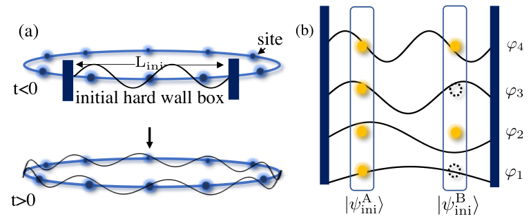
To test the accuracy of $\hat{\rho}_{\text{1NC}}$, we consider a concrete initial state and its dynamics under the Hamiltonian (8). As shown in Fig. 1(a), we suppose an initial hard wall box, which confines $N$ particles to the sites $1\leq i\leq L_{\mathrm{ini}}$ ($N\leq L_{\mathrm{ini}}$). The one-particle energy eigenstates within the box are $\varphi_{n}(j)=(L_{\mathrm{ini}}+1)^{-1/2}\sin[\pi nj/(L_{\mathrm{ini}}+1)]$ as illustrated in Fig. 1(b). Introducing the creation operators for these eigenstates as $\Phi_{n}^{\dagger}=\sum_{j=1}^{{\color[rgb]{0,0,0}L_{\text{ini}}}}\varphi_{n}(j)\hat{c}^{{\dagger}}_{j}$, we consider the following two initial states: the ground state $\ket{\psi_{\text{ini}}^{\text{A}}}=\prod_{n=1}^{N}\Phi_{n}^{\dagger}\ket{0}$ and an excited state $\ket{\psi_{\text{ini}}^{\text{B}}}=\prod_{n=1}^{N}\Phi_{2n}^{\dagger}\ket{0}$ (for $N\leq L_{\mathrm{ini}}/2$). We remove the hard wall instantaneously at time $t=0$, let these initial states evolve under $\hat{H}$, or freely expand into the entire $L$ sites, and analyze the long-time average of various observables.

Figure 2 displays the values of the additional conserved quantities $|\braket{\hat{J}_{k}}_{\text{ini}}|\equiv|\bra{\psi_{\text{ini}}}\hat{J}_{k}\ket{\psi_{\text{ini}}}|$ for $\ket{\psi_{\text{ini}}}=\ket{\psi^{\text{A}}_{\text{ini}}}$ and $\ket{\psi^{\text{B}}_{\text{ini}}}$. While $|\braket{\hat{J}_{k}}_{\text{ini}}|$ are almost zero for most $k$ in $\ket{\psi^{\text{A}}_{\text{ini}}}$, it has large values for $0<k<2\pi/3$ in $\ket{\psi^{\text{B}}_{\text{ini}}}$. Thus, $\hat{J}_{k}$ is less important for the GGE in case of $\ket{\psi^{\text{A}}_{\text{ini}}}$ and the generalized temperatures for $\hat{J}_{k}$ are almost zero for most $k$. On the other hand, in case of $\ket{\psi^{\text{B}}_{\text{ini}}}$, we should use $\hat{J}_{k}$ in the GGE and the generalized temperatures have large absolute values.

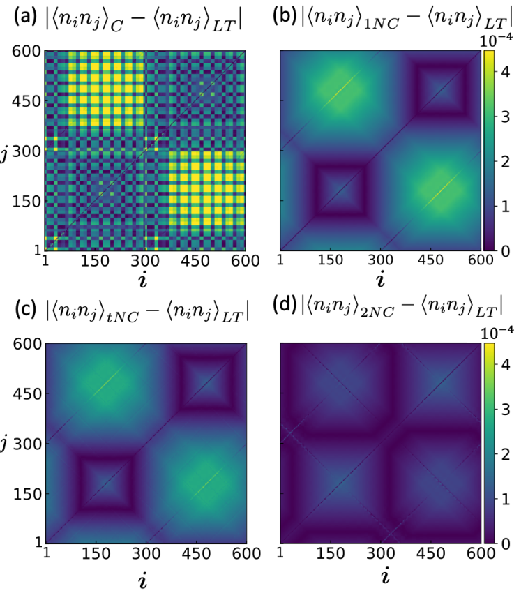
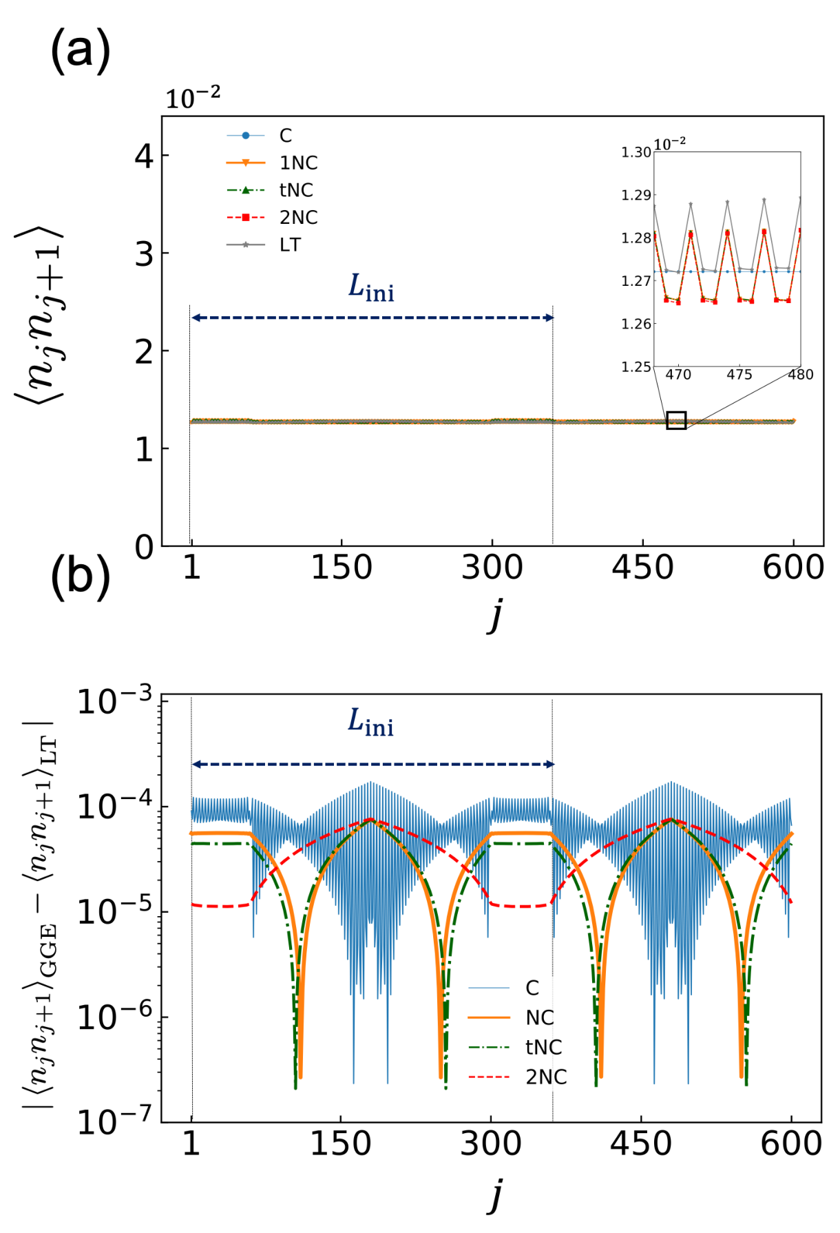
To compare the one-body NCGGE and the conventional CGGE, we consider some two-body observables since we have already shown that one-body observables are exactly described by the one-body NCGGE. To highlight the role of $\hat{J}_{k}$, we take $\ket{\psi_{\text{ini}}^{\text{B}}}$ as an initial state and focus on the density-density correlation $\hat{n}_{i}\hat{n}_{j}$ ($n_{i}\equiv\hat{c}^{{\dagger}}_{i}\hat{c}_{i}$) ¹¹ 1 We actually calculate the normal-ordered operator $:\!\hat{n}_{i}\hat{n}_{j}\!:\,=\hat{c}_{i}^{\dagger}\hat{c}_{j}^{\dagger}\hat{c}_{j}\hat{c}_{i}$ to remove the unwanted one-body contributions. and calculate the error of the GGEs $|\braket{\hat{n}_{i}\hat{n}_{j}}_{\mathrm{GGE}}-\braket{\hat{n}_{i}\hat{n}_{j}}_{\mathrm{LT}}|$, where $\mathrm{GGE}$ means the one-body NCGGE (1NC) or CGGE (C). We plot these errors in Figs. 3(a) and (b), finding $\hat{\rho}_{\text{1NC}}$ more accurate than the CGGE as a whole. We turn our attention further to local physical quantities $n_{j}n_{j+1}$, which are 1-local operators and the sub-diagonal components of Fig. 3. For a quantitative comparison of the local observables, we plot the expectation values of $\hat{n}_{j}\hat{n}_{j+1}$ in Fig. 4(a) and the errors of the GGEs $|\braket{\hat{n}_{j}\hat{n}_{j+1}}_{\mathrm{GGE}}-\braket{\hat{n}_{j}\hat{n}_{j+1}}_{\mathrm{LT}}|$ in Fig. 4(b). We find that $\hat{\rho}_{\text{1NC}}$ describes the long-time average $\braket{\hat{n}_{j}\hat{n}_{j+1}}_{\text{LT}}$ better than the CGGE for most $j$ in Fig. 4. It is noteworthy that the $\hat{\rho}_{\text{1NC}}$ captures the characteristic peaks of $\braket{\hat{n}_{j}\hat{n}_{j+1}}_{\text{LT}}$ while the CGGE cannot. These characteristic peaks are related to the inversion symmetry and not present for $\ket{\psi_{\text{ini}}^{\text{A}}}$ (see Appendix H), for which the improvement by $\hat{\rho}_{\text{1NC}}$.

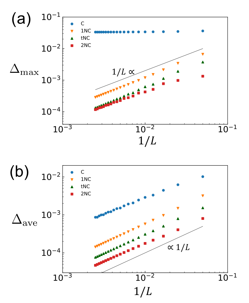
We also examine how the errors scale in the system size $L$ with ratios $N/L_{\mathrm{ini}}$ and $L_{\mathrm{ini}}/L$ held fixed. We define the averaged error of the density-density correlation by $\Delta_{\text{ave}}\equiv\sum_{j}|\braket{\hat{n}_{j}\hat{n}_{j+1}}_{\mathrm{GGE}}-\braket{\hat{n}_{j}\hat{n}_{j+1}}_{\mathrm{LT}}|/L$, which is plotted for GGEs at several system sizes in Fig. 5(b). The error is much smaller for $\hat{\rho}_{\text{1NC}}$, and decreases as $\propto 1/L$ to vanish in the thermodynamic limit for both GGEs ²² 2 This power-law decay is a feature of integrable models Biroli et al. 2010, and the error decays exponentially in nonintegrable models Beugeling et al. 2014; Ikeda and Ueda 2015. Thus, the CGGE also becomes accurate in this limit on average. However, when we use a more strict definition for the error defined by $\Delta_{\text{max}}\equiv\max_{j}|\braket{\hat{n}_{i}\hat{n}_{j+1}}_{\mathrm{GGE}}-\braket{\hat{n}_{j}\hat{n}_{j+1}}_{\mathrm{LT}}|$, we come to a different conclusion: the one-body NCGGE becomes accurate as $L\to\infty$ while the CGGE does not, as shown in Fig. 5(a). This is due to the characteristic peaks shown in Fig. 4 and the maximum error of the CGGE occurs at the high-symmetry points $j=L_{\text{ini}}/2$ and $(L_{\text{ini}}+L)/2$. For the other initial state $\ket{\psi_{\text{ini}}^{\text{A}}}$, as $L$ increases, $\Delta_{\text{max}}$ of the CGGE also decreases as $\propto 1/L$ because there are no characteristic peaks, which cannot be captured by the CGGE. These results show that the one-body NCGGE improves the GGE prediction quantitatively as a whole, but some of the local correlations such as $n_{L_{\text{ini}}/2}n_{L_{\text{ini}}/2+1}$ can be improved by one-body NCGGE qualitatively from the CGGE. The NCGGE can be necessary for accurately describing the actual stationary state even in the thermodynamic limit, depending on the initial state.

Introducing noncommutative sets of conserved quantities and the observable projection idea, we have systematically shown that the NCGGE describe the long-time behavior of isolated quantum systems better than the conventional CGGE. For noninteracting integrable systems, we have explicitly constructed the exact $N$-body NCGGE that describes the long-time average of up-to-$N$-body observables without an error even at finite system size. Besides, we have shown that the one-body NCGGE, the trigonal NCGGE, and the two-body NCGGE can be numerically implemented and describe two-body observables well. We note that the additional noncommutative conserved quantities are nonlocal. However, there exist local observables which need these nonlocal additional conserved quantities for qualitative description depending on the initial state.

The implementation of the NCGGE in interacting integrable systems is an important open problem. This problem is challenging because noncommutative sets of conserved quantities are not explored well in these systems and our approach presented for noninteracting systems does not apply. However, as we have remarked in Sec. III, one can numerically conduct the observable projection scheme for moderate system sizes and test whether the NCGGE is necessary or not. The numerical operator projection can be performed by the Gram–Schmidt orthogonalization and by the exact simultaneous diagonalization of the commutative local conserved quantities once we know the explicit form of the commutative local conserved quantities derived from the transfer matrix (see Appendix C for more details). With this analysis, we can see whether NCGGE is needed or not in interacting integrable systems. Moreover, we may even find new conserved quantities that do not commute with the well-known commutative ones.

Finally, we remark that the quantum-information-theoretic thermodynamics using noncommutative conserved quantities has attracted attention Yunger Halpern et al. 2016. An experimental protocol for its realization has been proposed in small nonintegrable systems Yunger Halpern et al. 2020. Our NCGGE arising in large integrable systems provides another route to the quantum-information-theoretic thermodynamics.

We thank H. Tsunetsugu for fruitful discussion and L. Piroli for his helpful comment on our manuscript. This work was supported by JSPS KAKENHI Grant No. JP18K13495. K.F. acknowledges support by the Forefront Physics and Mathematics Program to Drive Transformation (FoPM), WINGS Program, the University of Tokyo.

References

- D’Alessio et al. (2016) L. D’Alessio, Y. Kafri, A. Polkovnikov, and M. Rigol, Advances in Physics 65, 239 (2016).
- Eisert et al. (2015) J. Eisert, M. Friesdorf, and C. Gogolin, Nature Physics 11, 124 (2015).
- Ilievski et al. (2016) E. Ilievski, M. Medenjak, T. Prosen, and L. Zadnik, J. Stat. Mech. 2016, 64008 (2016).
- Mori et al. (2018) T. Mori, T. N. Ikeda, E. Kaminishi, and M. Ueda, Journal of Physics B: Atomic, Molecular and Optical Physics 51, 112001 (2018).
- Kinoshita et al. (2006) T. Kinoshita, T. Wenger, and D. S. Weiss, Nature 440, 900 (2006).
- Trotzky et al. (2011) S. Trotzky, Y.-A. Chen, A. Flesch, I. P. McCulloch, U. Schollwöck, J. Eisert, and I. Bloch, Nature Physics 8, 8 (2011) .
- Langen et al. (2013) T. Langen, R. Geiger, M. Kuhnert, B. Rauer, and J. Schmiedmayer, Nature Physics 9, 640 (2013).
- Langen et al. (2015) T. Langen, S. Erne, R. Geiger, B. Rauer, T. Schweigler, M. Kuhnert, W. Rohringer, I. E. Mazets, T. Gasenzer, and J. Schmiedmayer, Science 348, 207 (2015).
- Schreiber et al. (2015) M. Schreiber, S. S. Hodgman, P. Bordia, H. P. Lüschen, M. H. Fischer, R. Vosk, E. Altman, U. Schneider, and I. Bloch, Science 349, 842 (2015).
- Kaufman et al. (2016) A. M. Kaufman, M. E. Tai, A. Lukin, M. Rispoli, R. Schittko, P. M. Preiss, and M. Greiner, Science 353, 794 (2016).
- Tasaki (1998) H. Tasaki, Phys. Rev. Lett. 80, 1373 (1998).
- Reimann (2008) P. Reimann, Phys. Rev. Lett. 101, 190403 (2008).
- Linden et al. (2009) N. Linden, S. Popescu, A. J. Short, and A. Winter, Phys. Rev. E 79, 61103 (2009).
- Deutsch (1991) J.M. Deutsch, Phys. Rev. A 43, 2046 (1991).
- Srednicki (1994) M. Srednicki, Phys. Rev. E 50, 888 (1994).
- von Neumann (2010) J. von Neumann, The European Physical Journal H 237, 41 (2010) .
- Rigol et al. (2008) M. Rigol, V. Dunjko, and M. Olshanii, Nature 452, 854 (2008).
- Santos and Rigol (2010) L. F. Santos and M. Rigol, Phys. Rev. E 81, 036206 (2010).
- Kim et al. (2014) H. Kim, T. N. Ikeda, and D. A. Huse, Phys. Rev. E 90, 052105 (2014).
- Beugeling et al. (2014) W. Beugeling, R. Moessner, and M. Haque, Phys. Rev. E 89, 042112 (2014).
- Steinigeweg et al. (2014) R. Steinigeweg, a. Khodja, H. Niemeyer, C. Gogolin, and J. Gemmer, Phys. Rev. Lett. 112, 1 (2014), arXiv:1311.0169 .
- Khodja et al. (2015) A. Khodja, R. Steinigeweg, and J. Gemmer, Phys. Rev. E 91, 012120 (2015).
- Yoshizawa et al. (2018) T. Yoshizawa, E. Iyoda, and T. Sagawa, Phys. Rev. Lett. 120, 200604 (2018).
- Rigol et al. (2007) M. Rigol, V. Dunjko, V. Yurovsky, and M. Olshanii, Phys. Rev. Lett. 98, 50405 (2007).
- Biroli et al. (2010) G. Biroli, C. Kollath, and A. M. Läuchli, Phys. Rev. Lett. 105, 250401 (2010).
- Ikeda et al. (2013) T. N. Ikeda, Y. Watanabe, and M. Ueda, Phys. Rev. E 87, 012125 (2013).
- Alba (2015) V. Alba, Phys. Rev. B 91, 155123 (2015).
- Pal and Huse (2010) A. Pal and D. A. Huse, Phys. Rev. B 82, 174411 (2010).
- Iyer et al. (2013) S. Iyer, V. Oganesyan, G. Refael, and D. A. Huse, Phys. Rev. B 87, 134202 (2013).
- van den Worm et al. (2013) M. van den Worm, B. C. Sawyer, J. J. Bollinger, and M. Kastner, New J. Phys. 15, 083007 (2013).
- Shiraishi and Mori (2017) N. Shiraishi and T. Mori, Phys. Rev. Lett. 119, 30601 (2017).
- Mondaini et al. (2018) R. Mondaini, K. Mallayya, L. F. Santos, and M. Rigol, Phys. Rev. Lett. 121, 38901 (2018).
- Jaynes (1957) E. T. Jaynes, Phys. Rev. 106, 620 (1957).
- Vidmar and Rigol (2016) L. Vidmar and M. Rigol, J. Stat. Mech. 2016, 64007 (2016).
- Caux and Konik (2012) J.-S. Caux and R. M. Konik, Phys. Rev. Lett. 109, 175301 (2012).
- Pozsgay (2013) B. Pozsgay, Journal of Statistical Mechanics: Theory and Experiment 2013, P07003 (2013).
- Fagotti et al. (2014) M. Fagotti, M. Collura, F. H. L. Essler, and P. Calabrese, Phys. Rev. B 89, 125101 (2014).
- Wouters et al. (2014) B. Wouters, J. De Nardis, M. Brockmann, D. Fioretto, M. Rigol, and J.-S. Caux, Phys. Rev. Lett. 113, 117202 (2014).
- Pozsgay et al. (2014) B. Pozsgay, M. Mestyán, M. A. Werner, M. Kormos, G. Zaránd, and G. Takacs, Phys. Rev. Lett. 113, 117203 (2014).
- Ilievski et al. (2015) E. Ilievski, J. De Nardis, B. Wouters, J.-S. Caux, F. H. L. Essler, and T. Prosen, Phys. Rev. Lett. 115, 157201 (2015).
- Hamazaki et al. (2016) R. Hamazaki, T. N. Ikeda, and M. Ueda, Phys. Rev. E 93, 032116 (2016).
- Cardy (2016) J. Cardy, Journal of Statistical Mechanics: Theory and Experiment 2016, 23103 (2016).
- Kollar and Eckstein (2008) M. Kollar and M. Eckstein, Phys. Rev. A 78, 13626 (2008).
- Kollar et al. (2011) M. Kollar, F. A. Wolf, and M. Eckstein, Phys. Rev. B 84, 054304 (2011).
- Caneva et al. (2011) T. Caneva, E. Canovi, D. Rossini, G. E. Santoro, and A. Silva, J. Stat. Mech. 2011, P07015 (2011).
- He et al. (2013) K. He, L. F. Santos, T. M. Wright, and M. Rigol, Phys. Rev. A 87, 63637 (2013).
- Ziraldo et al. (2012) S. Ziraldo, A. Silva, and G. E. Santoro, Phys. Rev. Lett. 109, 247205 (2012).
- Ziraldo and Santoro (2013) S. Ziraldo and G. E. Santoro, Phys. Rev. B 87, 64201 (2013).
- Wang and Tong (2017) X. Wang and P. Tong, J. Stat. Mech. 11, 113107 (2017).
- Kaminishi et al. (2015) E. Kaminishi, T. Mori, T. N. Ikeda, and M. Ueda, Nature Physics 11, 1050 (2015).
- Fagotti (2014) M. Fagotti, J. Stat. Mech. 2014, P03016 (2014).
- Yukalov (2011) V. I. Yukalov, Physics Letters A 375, 2797 (2011).
- Short (2011) A. J. Short, New J. Phys. 13, 53009 (2011).
- Reimann and Kastner (2012) P. Reimann and M. Kastner, New J. Phys. 14, 043020 (2012) .
- Cassidy et al. (2011) A. C. Cassidy, C. W. Clark, and M. Rigol, Phys. Rev. Lett. 106, 140405 (2011).
- Mierzejewski and Vidmar (2020) M. Mierzejewski and L. Vidmar, Phys. Rev. Lett. 124, 40603 (2020).
- (57) We actually calculate the normal-ordered operator to remove the unwanted one-body contributions.
- (58) This power-law decay is a feature of integrable models Biroli et al. 2010, and the error decays exponentially in nonintegrable models Beugeling et al. 2014; Ikeda and Ueda 2015.
- Yunger Halpern et al. (2016) N. Yunger Halpern, P. Faist, J. Oppenheim, and A. Winter, Nature Communications 7, 12051 (2016).
- Yunger Halpern et al. (2020) N. Yunger Halpern, M. E. Beverland, and A. Kalev, Phys. Rev. E 101, 42117 (2020).
- Golden (1965) S. Golden, Phys. Rev. 137, B1127 (1965).
- Ikeda and Ueda (2015) T. N. Ikeda and M. Ueda, Phys. Rev. E 92, 020102(R) (2015).