Quantum to classical crossover of Floquet engineering in correlated quantum systems
Abstract
Light-matter coupling involving classical and quantum light offers a wide range of possibilities to tune the electronic properties of correlated quantum materials. Two paradigmatic results are the dynamical localization of electrons and the ultrafast control of spin dynamics, which have been discussed within classical Floquet engineering and in the deep quantum regime where vacuum fluctuations modify the properties of materials. Here we discuss how these two extreme limits are interpolated by a cavity which is driven to the excited states. In particular, this is achieved by formulating a Schrieffer-Wolff transformation for the cavity-coupled system, which is mathematically analogous to its Floquet counterpart. Some of the extraordinary results of Floquet-engineering, such as the sign reversal of the exchange interaction or electronic tunneling, which are not obtained by coupling to a dark cavity, can already be realized with a single-photon state (no coherent states are needed). The analytic results are verified and extended with numerical simulations on a two-site Hubbard model coupled to a driven cavity mode. Our results generalize the well-established Floquet-engineering of correlated electrons to the regime of quantum light. It opens up a new pathway of controlling properties of quantum materials with high tunability and low energy dissipation.
I Introduction
Under a time-periodic perturbation, such as the electric field of a laser or a coherently excited phonon, the time-evolution and steady states of a quantum system are described by an effective time-independent Floquet Hamiltonian , which can be entirely different from the undriven one. Mathematically, is defined through the stroboscopic time-evolution over a period of the drive. The design of a given Floquet Hamiltonian with suitable driving protocols, termed Floquet engineering Bukov et al. 2015a; Eckardt 2017; Oka and Kitamura 2019, has become an important tool for quantum simulation with ultracold gases, and it has been widely discussed in relation to the control of interactions and phase transitions in solids. A certainly incomplete list of theoretical proposals includes the manipulation of topologically nontrivial bands Oka and Aoki 2009; Lindner et al. 2011, spin Hamiltonians Mentink et al. 2015; Claassen et al. 2017; Kitamura et al. 2017, superconductors Raines et al. 2015; Höppner et al. 2015; Kitamura and Aoki 2016; Sentef et al. 2016; Knap et al. 2016; Sentef et al. 2017; Kennes et al. 2017; Murakami et al. 2017; Wang et al. 2018; Sheikhan and Kollath 2019; Tindall et al. 2019, strongly correlated materials Tsuji et al. 2011; Tancogne-Dejean et al. 2018; Walldorf et al. 2019; Kennes et al. 2018; Peronaci et al. 2020; Takasan et al. 2017 and magnetic topological phase transitions Topp et al. 2018.
A major limitation to Floquet engineering is heating. The generic steady state of an isolated periodically driven many-body system is an infinite-temperature state D’Alessio and Rigol 2014; Lazarides et al. 2014, and although interesting Floquet phases may emerge as prethermal states Weidinger and Knap 2017; Canovi et al. 2016; Abanin et al. 2015; Dasari and Eckstein 2018; Herrmann et al. 2017; Bukov et al. 2015b, many of the above-mentioned theoretical predictions have not been implemented in solids. Even in cold atom systems, heating can be substantial Sandholzer et al. 2019; Reitter et al. 2017; Weinberg et al. 2015. In particular, the qualitatively most interesting effect on many-body interactions is typically achieved by driving a system close to a resonance, like phonon frequency for superconducting pairing Knap et al. 2016, or the Mott gap for the magnetic super-exchange Mentink et al. 2015, but this near-resonant regime is also where heating is most substantial Murakami et al. 2017.
On the other hand, quantum fluctuations of photon fields in cavities open the possibility to change the properties of matter through light-matter coupling without the need of strong lasers. In particular cavities have the advantage that strong light-matter coupling is in principle achievable, much stronger than the bare coupling in free space. Cavity quantum-electrodynamical environments therefore provide a new paradigm for using light-matter interactions for the creation of effective Hamiltonians with tunable interactions, with intriguing proposals ranging from light-induced superconducting pairing to magnetic super-exchange or ferroelectricity Hagenmüller et al. 2017; Sentef et al. 2018; Schlawin et al. 2019; Curtis et al. 2019; Mazza and Georges 2019; Andolina et al. 2019; Kiffner et al. 2019a; Rokaj et al. 2019; Wang et al. 2019.
While such a control of many-body interactions has been discussed mostly in the deep quantum limit, where vacuum fluctuations alone affect the solid, one can anticipate that driving the cavity state out of equilibrium implies a continuous crossover to the classical limit of Floquet engineering. Simply speaking, this crossover is expected to exist because both in the quantum limit and in the Floquet limit the many-body system can exchange photons with the light field, giving rise to induced interactions between the low energy degrees of freedom. In the quantum limit, an example for effective electronic interactions mediated by a vacuum of bosons can be found in the well-known Bardeen-Cooper-Schrieffer mechanism for phonon-mediated electron-electron attraction, which comes about through the exchange of virtual phonons between electrons. Similarly, induced interaction still emerge when the bosonic field is excited, and populated with states of few photons or phonons or superpositions thereof. In this case both virtual photon emission and absorption contribute to the induced interaction. Classical laser fields finally correspond to coherent states of high photon numbers, so one can anticipate that the induced interactions in the Floquet Hamiltonian arise when virtual photon absorption and emission become entirely symmetric. This will be explicitly shown below.
The basic question to be asked here is whether one can, at strong coupling, achieve with only few photons a similar renormalization of the Hamiltonian as in the classically driven case. Because heating is intrinsically related to the presence of an infinite energy density in the photon system, it should be less relevant if only few photons partake. Naively one might assume that the classically driven Floquet limit is recovered only when the cavity is put in a coherent state, but, as we will explain in this work, this is not generally true: At strong light-matter coupling, a Hamiltonian similar to the Floquet Hamiltonian can be engineered by putting the cavity in a given photon-number state (with zero expectation value of the driving field), while a coherent state will lead to a more complicated dynamics which is not described by a single effective matter Hamiltonian.
In this paper, we address this fundamental question by demonstrating the crossover from cavity-coupling to coherent Floquet engineering for two important classes of Floquet problems: (i) The renormalization of tunnelling (dynamical localizaton) Shirley 1965; Dunlap and Kenkre 1986, which underlies the Floquet band-structure control, and (ii), effective induced interactions such as kinetic spin exchange emerging from mobile electrons with Coulomb repulsion, which can be obtained from the Schrieffer-Wolff transformation. The Schrieffer-Wolff transformation is a perturbative framework to derive effective interactions in a sub-Hilbert space, when the rest of the states is projected out; its application includes the derivation of spin models, the -model, phonon-mediated electron-electron interactions, and more Bravyi et al. 2011. The Floquet-Schrieffer-Wolff transformation Bukov et al. 2016 is therefore an equally powerful approach to understand the design of induced interactions under periodic driving. Here we present a formulation of the Schrieffer-Wolff transformation of the light-matter Hamiltonian which is in close analogy to the Floquet-Schrieffer-Wolff transformation, and thus shows how the Floquet induced interactions are approached by the induced interactions in the cavity when the photon number is increased .
The Schrieffer-Wolff transformation is mathematically similar for different systems, and we investigate it for the paradigmatic example of the spin exchange interaction. The classically driven system has been examined in photo-excited solid-state materials as well as shaken cold-atom systems Mikhaylovskiy et al. 2015; Desbuquois et al. 2017; Görg et al. 2018, and provides an interesting route both for designing exotic spin models Claassen et al. 2017 and for the ultrafast control of magnetism Mentink 2017; Kirilyuk et al. 2010. While in the Floquet limit it is possible to reverse the sign of the interaction Mentink et al. 2015 (as experimentally observed in Görg et al. 2018), vacuum fluctuations alone only reduce the exchange Kiffner et al. 2019a. Here we will see that already a single photon can be enough to allow for the sign-reversal of the interaction and almost quantitatively restore the classical Floquet limit.
This paper is organized as follows. In Sec. II, we discuss the cavity-coupled Hubbard model and the crossover of the dynamical localization phenomenon into the quantum regime. In Sec. III, the Schrieffer-Wolff transformation is discussed for a two-site Hubbard model and a corresponding spin-photon Heisenberg model is derived at large . In Sec. IV, we discuss the high-frequency limit of the cavity-Heisenberg dimer, and consider its crossover from the Floquet driving limit, where the photon number approaches infinity, to the extreme quantum light regime where only a few photons are present in the cavity. Section V supplements the previous discussion with a numerical solution of a minimal model for a driven cavity, where cavity photons are created through an external classical driving, and Sec. VI includes the conclusion and outlook.
II Cavity-induced dynamical localization
In a certain sense, the link between classically driven Floquet systems and quantum systems is rather straightforward. Consider a Hamiltonian depending on a classical driving field . Floquet states are given by a Bloch wavefunction in time, , where the is periodic in time (). If expanded in a Fourier series, , the coefficients can be viewed as a wavefunction in a product space of matter states and a Floquet index , and the Floquet states are obtained from a solution of the time-independent Schrödinger equation with a Hamiltonian , known as the Floquet matrix. On the other hand, if the drive is replaced by the displacement of a quantum oscillator, , one can project the Hamiltonian on photon numbers. In the following, we will demonstrate that the Floquet Hamiltonian emerges as a classical limit, , when the photon number is large and the coupling is small,
| (1) |
Indeed, this statement already indicates that at strong light-matter coupling, states with few photons may be sufficient to realize effective Hamiltonians similar to the Floquet Hamiltonian. The structural similarity between the Floquet matrix and cavity quantum electrodynamics has been considered in ab initio calculations Schäfer et al. 2018; Hübener et al. 2020.
To concretely demonstrate the crossover from classical Floquet driving to the quantum light regime, we consider a 1D tight-binding model coupled to a single cavity mode. We assume the long-wavelength limit, i.e., the photon wavelength is much larger than the system size, so that one can make the dipole approximation. The cavity photon is described by a vector potential , where is a dimensionless light-matter coupling strength determined by the cavity setup and the operator annihilate/create a photon in the mode. With the electronic annihilation (creation) operators acting on site and spin and the number operator , the minimal gauge-invariant Hamiltonian is given by
| (2) |
Here is the electronic hopping matrix element between neighboring atoms, and denotes the bare cavity photon frequency. This minimal gauge-invariant model can also be derived from the microscopic description under certain circumstance Li et al. 2020 and is in line with the Peierls substitution in the semi-classical limit. It is worth noting that an expansion in powers of has been used to yield a bilinear term coupling the photonic displacement to the electronic bond current (“paramagnetic term”) in related works Kiffner et al. 2019a; Schlawin et al. 2019, which should be fine in the weak or intermediate coupling limit. For larger coupling, a next-leading term that is second order in and couples the squared vector potential to the kinetic energy of the electrons (“diamagnetic term”) can play a crucial role Kiffner et al. 2019b. Even in the weak light-matter coupling limit, a many-photon state may still feature a large amplitude , and the perturbation theory breaks down. In fact, this is nothing but the semiclassical limit discussed in the introduction. As we intend to make a bridge between these extreme regimes, we keep the exponential to all orders in the following.
From the Hamiltonian (2), taking a proper semi-classical limit at should recover the phenomenology of a Floquet driven system. In the latter case, the cavity mode should be replaced by a coherent electric field , leading to the Hamiltonian
| (3) |
where are the amplitude and frequency of the periodic external field. The effective Floquet Hamiltonian in the high-frequency limit is known to have a renormalized hopping Dunlap and Kenkre 1986; Bukov et al. 2015a
| (4) |
where is the zeroth Bessel function of the first kind.
We now concentrate on the corresponding renormalization of hopping due to the cavity photons in the high frequency limit. Specifically, we perform a unitary transformation on the cavity-lattice Hamiltonian (2) to enter the rotating frame (equivalent to going to the interaction picture with respect to ). This removes the term , and leads to the replacement . The transformed Hamiltonian is then periodic in time , and one can perform a high-frequency expansion Bukov et al. 2015a. The effective Hamiltonian at the lowest order, , is
| (5) |
where . (For details, see appendix A.1). When photons are present in the cavity, one can see that the electronic hopping is renormalized by a factor , i.e., . Finally, under the classical limit defined in Eq. (1), one can show that this renormalized hopping approaches the Floquet limit,
| (6) |
The Floquet-cavity crossover for dynamical localization is explicitly illustrated in Fig. 1. Panel a) shows the effective energy band with dispersion for different ( fixed). In the large limit the energy band becomes almost flat, which is consistent with the Floquet limit where for the given parameters. Figure 1b shows the renormalized hoppings as a function of the coupling. In the dark cavity (), the factor always leads to a reduced bandwidth , while the Floquet drive allows for a flipping of the band, with interesting consequences in interacting systems Tsuji et al. 2011. With more photons in the cavity (), both emission and absorption of virtual photons contribute to . It is interesting to see that a single photon is already sufficient to flip the band and thus correct for the qualitative difference between the dark cavity and the classically driven system.
As emphasized in the introduction, the Floquet Hamiltonian is recovered when the cavity is in a number state, and no coherent state is assumed. At small coupling and large photon number , however, the photon number state and a coherent state would nevertheless give the same result, because the coherent state has a small variance in the photon number . In the classical limit, therefore, the Floquet Hamiltonian can be realized by coherent driving. At large coupling and small photon number, in contrast, the coherent state would give an dynamics which cannot be described by a single tunnelling matrix element at all. This will be illustrated in more detail for the following example.
III Schrieffer-Wolff transformation in the cavity
In this section we extend the Hamiltonian (2) by a local Hubbard interaction ,
| (7) |
We will take this as an example to discuss the cavity to Floquet crossover regarding induced interactions in a low-energy space. For this purpose, we focus on the limit at half filling (one electron per site). In this limit, it is well known that the effective low-energy Hamiltonian without coupling to the electromagnetic field is obtained by projecting out configurations which contain doubly occupied and empty sites (Schrieffer-Wolff transformation). The resulting low energy space has one spin-1/2 at each lattice site, and the effective Hamiltonian is a Heisenberg model with exchange interaction ( are canonical spin- operators). In the following we include the coupling to the electromagnetic field, but still focus on the limit and ask how the low-energy spin model and the induced spin interactions are modified by either classical driving (replacing as in the previous section) or by coupling to the quantum field, and how the two limits are related. For this purpose it is sufficient to consider a minimal Hubbard lattice of two sites (Hubbard dimer).
With the coupling to the cavity mode, the relevant Hilbert space at , after projecting out electronically excited doubly occupied states, will contain both spins and photons, and the effective Hamiltonian is therefore a spin-photon model. Below we will derive a suitable Schrieffer-Wolff transformation for the electron-photon Hamiltonian (7) to show that the Hubbard dimer reduces to the spin-photon Heisenberg model
| (8) |
where the exchange interaction becomes an operator acting on the photon states. In deriving this expression, we only assume the absence of (multi-photon) resonances, i.e., for any integer . It is convenient to separate into photon number transitions,
| (9) | ||||
| (10) |
where are (normal ordered) hermitian operators which are diagonal in the photon number, , and the overall scale is the bare kinetic exchange interaction . Note that only even photon number transitions have non-vanishing matrix elements. The function contains the dependence of the exchange interaction on frequency. Its precise form is given in the appendix in Eq. (A59). It is a smooth function of and , apart from divergencies at the resonances , with integer .
The above equations constitute a central result of this paper. The spin-photon Hamiltonian has a similar form to the Floquet-engineered spin Hamiltonian described below, but describes the full dynamics of the spin and photon-coupled system. In Eq. (10) the non-resonance condition is assumed , but no assumption is made for the relation between and the low energy scale , leaving the full photon dynamics intact. Thus, the Hamiltonian describes both the photon-engineered spin dynamics, and the modification of photon states due to the presence of magnetic degrees of freedom. In the following we briefly discuss the renormalization of the photon states, and then turn to the cavity-engineering of the spin-exchange coupling.
Below we contrast these results to the Floquet-driven system. The Floquet spin Hamiltonian at has been obtained in the same spirit as the Heisenberg model above, by assuming that the non-resonant driving does not generate charge excitations, and one can thus project out doubly occupied states from the Floquet Hamiltonian Mentink et al. 2015. Alternative derivations have been formulated in various ways, including operator-based Floquet Schrieffer-Wolff transformations Bukov et al. 2016, time-dependent Schrieffer Wolff transformations Eckstein et al. 2017, or a resummation of the high-frequency expansion Itin and Katsnelson 2015. For , the low-energy physics of the Floquet-driven system is described by the Floquet Heisenberg model , with exchange interaction given by Mentink et al. 2015
| (11) |
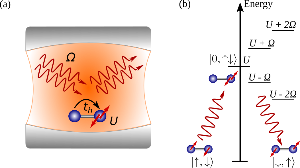
with being the exchange interaction of the undriven system and being the th Bessel function. This expression can be schematically explained with the multiple Floquet sectors with energy , for , contributing to the virtual spin exchange process, as shown in Fig. 2(b). Note that is needed to exclude real photon emission/absorption in the effective model (11). In the undriven case , the usual Heisenberg model is restored as .
Analogously, we consider the limit of the cavity-Hubbard dimer (7). In this limit, the induced magnetic interaction () emerges due to electron hopping between neighboring lattice sites with an intermediate excited state. For example, one electron (say spin up) at site 1 can hop to its neighbor 2 and form a spin singlet (the doublon) at 2. If photons are absorbed (emitted) in this process, the intermediate state then has excess energy , respectively. The other electron (spin down) can eventually hop back to site 1, with the net result of exchanging the two spins. If the high-frequency limit is taken, the absorbed (emitted) photon have to be emitted (absorbed) back, and the system must go back to the original photon-number state. This is in parallel with the Floquet scenario as discussed above. However, in that case the energy is borrowed from (or lent to for negative ) the classical driving field, instead of the quantized cavity levels.
We briefly describe here how to systematically derive the effective model Eq. 8 and refer to Appendix A for details. One again applies the unitary transformation and separate the Hilbert space into sectors and without and with charge excitations (doublons, holes), respectively. No assumption is made on , and both sectors may contain an arbitrary number of photons. It is then possible to perform a subsequent time-periodic unitary transformation, analogous to the Floquet Schrieffer-Wolff transformation, such that the coupling matrix elements between the two sectors are small in , and after that project to the sector . This procedure is essentially a generalized Schrieffer-Wolff transformation in the electron-photon Hilbert space. Details of this cavity Schrieffer-Wolff transformation can be found in Appendix A.
Squeezed photon states
In general, the photon states are coupled to magnetic excitations in the spin-photon Heisenberg model. For the dimer, the eigenfunctions are obtained in the form , where is the spin wave function, which is a singlet () or triplet (), and is the eigenfunction of the operator . The operator contains various photon nonlinearities. For example, it can be readily evaluated at weak coupling
| (12) | ||||
| (13) |
so that the cavity wave functions for are squeezed, and the cavity frequency is shifted. Figure 3 shows the energy shift relative to the free photon . The results are obtained by diagonalizing . At small the shift of the cavity frequency is proportional to . For larger nonlinearities (photon self-interaction) set in. The results obtained in the high-frequency limit, omitting the photon-non-diagonal terms in the Hamiltonian, are shown in the figure with dashed lines. The high-frequency expansion is reasonable when (lower panel). In contrast, when , the photon ground wave function becomes a squeezed state, with admixtures from .
It is worth noting that the Schrieffer-Wolff transformation can be performed for the Hubbard model on an arbitrary lattice,
| (14) |
where is determined by the exchange operator of the two-site model with the hopping and coupling for the given bond. On an arbitrary lattice, spin excitations can be created through photon absorption, or vice versa. For example, if the polarization is such that only bonds along one direction of the lattice are affected, the Hamiltonian gives rise to two-magnon two-photon scattering terms. The discussion of this rich physics is left for future works.
IV The Cavity-Floquet crossover
IV.1 Floquet crossover of the photon-number states
We now turn to the cavity-engineering of the spin dynamics in the high-frequency limit where one can project out the creation and annihilation of real photon excitations. We emphasize that, distinct from the case of dynamical localization, the frequency does not have to be high compared to the energy scales or which have already been removed from the Hamiltonian. In the high-frequency limit one could perform another unitary transformation, which rotates away the transition matrix elements between different photon number sectors. This would result in corrections of order to the photon-diagonal exchange Hamiltonian, which are omitted 11 1 For example, if and are of the same order, is of order , and should thus be omitted consistent with the lowest order expansion in .. The resulting exchange operator thus becomes photon diagonal, and the full Hamiltonian becomes
| (15) |
with , and an exchange interaction . Analogous to the dynamical localization [Eq. (6)], one can now show explicitly that in the classical limit (1), the exchange interaction approaches the Floquet result (11) (see appendix A.1 for details),
| (16) |
The behavior of , which quickly converges to the Floquet limiting curves (dashed lines) as rises, is systematically demonstrated in Fig. 4. For small , the red-detuned () cavity results in an enhanced while the blue-detuned () cavity leads to a reduced , and eventually a sign change. In the case of a completely dark cavity (), is suppressed for both red and blue-detuned frequencies, and is thus qualitatively different from the Floquet limit . Similar to the case of dynamical localization, however, a single photon is already sufficient to resolve these qualitative differences, and in particular restore the possibility to flip the sign of the exchange interaction. Also quantitatively, we observe a rather fast convergence of with the photon number.
Note that the qualitative enhancement and suppression of in the red- and blue-detuned cases are consistent with the result of Ref. Kiffner et al. 2019b based on an expansion of the light-matter coupling truncated at the quadratic “diamagnetic” term. The suppression in the blue-detuned case is, in particular, missing in the linear coupling approximation (“paramagnetic” term) Kiffner et al. 2019a.
IV.2 The spin dynamics in the high-frequency limit
While at strong coupling the Floquet exchange is recovered with only few photons, it should be emphasized that putting the cavity in a coherent state does not necessarily recover the Floquet result. Instead, the resulting dynamics of the spin subsystem cannot be described by a single spin Hamiltonian at all. In this section we illustrate this fact with a simple precessional spin dynamics: We prepare the system in a state
| (17) |
where the spins form a Neel state , which is a singlet-triplet superposition, and the cavity is in an arbitrary state. Then we find for the precessional motion of the spin on site ,
| (18) |
The behavior (18) of the cavity-driven Heisenberg dimer is therefore apparently different from the classical Floquet engineering. In the latter case, upon projecting out high-frequency processes, the Neel state would precess with a single renormalized frequency ,
| (19) |
This discrepancy is somehow expected as the coupling to a classical field is fundamentally distinct from the coupling to a few discrete quantum states, where multiple precessional frequencies can emerge out of the coupling to a plethora of discrete levels.
To make a clear connection with the Floquet-driven case, we suppose the cavity is prepared in a coherent state with a mean number of photons, i.e.
| (20) |
Note that, by identifying with in the free field limit, one obtains the semiclassical correspondence . In Fig. 5, we examine the Fourier spectrum of the spin dynamics (18) for a coherent state with : , where is a broadened peak with frequency resolution . At different cavity coupling , we plot the Fourier spectrum and compare it to the Floquet exchange . The large limit is obtained by taking a small with a fixed amplitude . It is evident that, with a relatively large (such as in the figure), the Fourier spectrum fits very well with the Floquet limit. This is expected as in the semiclassical limit, the cavity-induced modification of should be consistent with the Floquet theory. For larger , at given , the photon number is small and we observe quantized frequency plateaus in the Fourier spectrum. The plateaus are generally in the vicinity of the Floquet curve . It is especially intriguing to see that, in the strong light-matter coupling limit, even with few photons, ( at for ) the discrete frequency levels still follow closely the Floquet curve . This extends the Floquet-like engineering into the few-photon, or extreme quantum light regime. As increases, the photon number increases for fixed , and the plateaus become denser and eventually merge into a continuum in the large limit. For a coherent state , the standard deviation of is and thus the sum (18) is dominated by the term . Therefore, the conventional Floquet engineering is restored in the coherent driving limit. We conclude that the two seemingly distinct situations, coupling to coherent driving and to a photon-number state, both converge to the Floquet-driven scenario in the semi-classical limit. The above discussion also shows that the modification of exchange interaction can be generalized to an arbitrary photon occupation provided is sharply centered around , without the assumption of a coherent or even a pure cavity state.

V Driving the cavity
Using the generalized Schrieffer-Wolff transformation, we have shown that both coherent states and photon-number states result in Floquet-like modifications of the magnetic dynamics. In more realistic experiments, the cavity would be driven to an excited state by some external field. In addition, the cavity is generically open and dissipative. In the following we consider a minimal setup of a driven cavity, where the cavity is originally prepared in the ground state (a dark cavity) and then is acted on by a time-dependent external laser field linearly coupled to the photon mode
| (21) |
so that the time evolution is determined by the total Hamiltonian
| (22) |
A closed and isolated cavity is still assumed, so that no dissipation or photon leakage is present in the time-evolution. Below we use a driving field
| (23) |
with driving frequency and amplitude .
We perform an exact time evolution with a truncated bosonic Hilbert space Sentef 2017 for the the case of a Hubbard dimer. In order to specifically address the photodressing effects on the effective magnetic exchange interaction we compute the local double-time spin-spin correlation function on the first site equal to the one on the second site,
| (24) |
where
| (25) |
denotes the wave function at time , and is the unitary time evolution operator with time ordering that propagates the wave function from the initial ground state of the undriven Hamiltonian to the time-evolved state,
| (26) |
From the double-time response function we compute a time- and frequency-resolved spin susceptibility
| (27) |
with probe envelope function
| (28) |
with probe duration and probe time . Note that for a pure Heisenberg dimer, , and therefore has a single peak at which directly measures .
Below we show results for runs up to , probe time and probe duration . The units are chosen such that the hopping sets the unit of energy, and correspondingly times are measured in units of . We note that , implying that for the time unit is . Throughout we fix to be in a relatively strong-coupling limit, for which the spin exchange interaction is perturbatively given by . We employ driving frequencies on resonance with the bare cavity mode frequency and choose these frequencies to be well above the scale, but on the order of .


We first investigate the spin susceptibility as a function of the dimensionless light-matter coupling . In practice, depends on the effective cavity volume and can be tuned by the specific cavity setup Maissen et al. 2014; Schlawin et al. 2019. Here we take it as a theory parameter to show the general effect of moderate light-matter coupling, which is realistically achievable. In Fig. 6 the top blue-colored curves show the spin susceptibility as a function of energy for the undriven cavity and coupling strengths and a blue-detuned cavity frequency, equal to the driving frequency, . Initially the peak position is 0.472, which corresponds to the bare exchange coupling and is slightly below the perturbative value . When is increased, the peak moves to smaller values, e.g., for .
Starting from we then turn on the external driving field . The evolution of the spin susceptibility under increasing shows that the peak position is further decreased. At the same time the curves broaden considerably. We note that a decrease of for blue-detuned driving is similarly obtained in the fully classical Floquet limit (11) Mentink et al. 2015.
To complement this behavior, we show in Fig. 7 the spin susceptibility evolving for sub-resonant, red-detuned frequency . First, for the dark cavity we observe again a reduction of , which is slightly less strong with compared to the blue-detuned case here. For instance, at we obtain compared to for the blue-detuned case. However, when the classical driving field is turned on, this reduction is quickly reversed and an enhancement of is obtained, consistent with the analytical results discussed above in the paper. At larger driving fields, not only a broadening is found, but also the emergence of sidepeaks in the spin susceptibility.

We summarize our findings for modifications of the effective exchange couplings in the driven cavity in Fig. 8, in which we show the extracted main peak positions as a function of the time-averaged photon field amplitude . First of all, the maximally achieved amplitudes are larger for the same set of external field values in the red-detuned case, which is attributed to the different modifications of photon frequencies for and cases, see Eq. 13 and the appendix B for details. Note that a similar dependence of on photon number instead of has also been found, which is expected because, as discussed in the analytical theory, a coherent displacement is not needed to modify the exhange interaction. The reduction (enhancement) of for blue (red) detuning is clearly visible here, and we find a quadratic dependence of this reduction (enhancement) on the driving-induced photon field amplitude, again consistent with the analytical results as well as the classical Floquet limit.
However, a quantitative comparison is more difficult. First of all, the initial ground state features a mixture of different photon-number states instead of a a single one, so that the spin dynamics is not described by a single spin Hamiltonian, but is a result of contributions from all photon number sectors. More importantly, the classical driving itself further mixes different photon-number states during the time-evolution, averaging over the frequency peaks in the Fourier spectrum. This renders a quantitative analysis, though possible with the analytic theory (calculating the time-evolution using the spin-photon hamiltonian (8)), complicated and less relevant in this minimal model. Thus we reserve it for future studies with a more realistic cavity setup.
Finally, we comment on the experimentally relevant effects of decoherence and dissipation in the case of a driven cavity, which are not included in the our simulations of a closed electron-photon system. First of all, one should state that these effects will result mainly from coupling to other degrees of freedom in the material under consideration, such as phonons or a substrate , and the resulting thermalization of the electronic system may stimulate photon absorption from the driven cavity. Cavity losses can also play a role but usually occur on longer time scales. It is clear that such decoherence and dissipation effects might limit the time scales on which cavity-modified exchange interactions will be achievable in practice. On the other hand, one of our central results is that coherence in the photon states is not a necessary prerequisite to achieve such cavity-modified interactions, provided that relatively strong light-matter coupling can be achieved. Therefore we expect the limitations of decoherence to be more severe at weak light-matter coupling than at strong light-matter coupling.
VI Conclusion and Outlook
In this work, we have investigated the light-induced changes in material properties from the quantum to the classical limit. In general, the classical limit is achieved by increasing the photon number , while decreasing the coupling, so that is fixed. We have introduced a cavity Schrieffer-Wolff transformation to derive the spin-exchange interaction in the presence of quantum light coupling. In particular, we observed that the cavity-modified spin-exchange interaction deviates from the bare value and matches both the Floquet result Mentink et al. 2015 in the classical limit, and the vacuum renormalization of Kiffner et al. 2019a for the dark cavity. By systematical examination of the quantum-light regime, we show that the Floquet engineering can be extended to the few-photon regime. In particular, already putting the cavity in the one-photon state is enough to revert the sign of , which is possible in the Floquet limit but not for the dark cavity.
A coherent amplitude of the photon field is not needed to recover the Floquet physics. Instead, if the cavity is in a coherent state with few photons, the dynamics of the matter is not described by a single effective Hamiltonian but instead shows individual contributions from each photon number sector. In the classical limit of weak coupling and macroscopically large photon number, on the other hand, both the photon number state and the coherent state, and in fact any photon occupation sharply centered around some large average photon number , recovers the Floquet limit. As a result, the assumption of a coherent driving is apparently too strong for the purpose of Floquet engineering. The slightly counterintuitive observation may be clarified by the fact that the effective exchange interaction in a classical coherent state is also obtained by virtual emission and absorption of photons. The phase information between the different Fock state components of the cavity state is thereby lost because a phase on emission is cancelled by a corresponding phase on absorption.
Moreover, we studied a minimal numerical model, where the cavity is driven by a classical field. In this minimal setup, the cavity acts as a transducer from the external driving laser to the electrons in a material. A photon amplitude is created by the external driving, and then drives the electronic system to modify its the spin susceptibility. The cavity-induced modification observed in the simulation is fully consistent with the analytic solution on the coherent state and photon-number state. It is shown that the Floquet-like engineering is indeed restored with a relatively weak photon amplitude, in the strong light-matter coupling regime. In contrast to the Floquet limit where excess heating is often unavoidable, a state with finitely many photons can minimize the heating effect, due to the limited electromagnetic energy inside the cavity volume. Our findings therefore open up new design opportunities for electronic devices with high tunability, low energy consumption, and minimal heating effects.
On the fundamental side, it will be also intriguing to further investigate how the control of induced interactions in solids by coupling to driven cavities can tune properties of quantum materials. In the future, it would be promising to extend the current results to a lattice model to examine the nature of mixed photon-magnon excitations. For example, the study of cavity-modified spin fluctuations and their influence on high-temperature superconductivity promises intriguing insights Dahm et al. 2009; Keimer et al. 2015. Using the cavity-Schrieffer Wolff transformation, it will also be interesting to investigate the Kondo physics and generally quantum criticality in the cavity-coupled system, as well as to look for cavity realizations of light-induced scalar spin chirality proposals Claassen et al. 2017; Kitamura et al. 2017; Owerre 2017; Elyasi et al. 2019 with time-reversal symmetry-breaking photon fields Wang et al. 2019. Another direction would be to study more realistic models, especially to include the effect of an open cavity, where a non-equilibrium steady-state of the light-matter system can be maintained through weak external driving.
Moreover, it will be interesting to consider long-range interactions induced via the cavity. In Ref. Kiffner et al. 2019a, such terms appear in form of hopping processes on two distant bonds which become correlated via virtual photon exchange. While such terms are not present in the spin model, where all charge excitations have been projected out, in the spin model one can expect corresponding correlated spin flips on distant bonds. To systematically derive such terms, one would have to go to fourth order perturbation theory in the hopping, which is possible, but left for future work. A subset of these terms, proportional to , can be obtained by perturbatively eliminating the two-photon creation and annihiliation processes from the spin-photon Hamiltonian. Though such terms are smaller in , their long-range character might make them highly relevant for the resulting spin models, in particular as long range spin interactions can give rise to frustration.
The discussion of cavity-Floquet crossover can also be extended to more general contexts, such as in the intermediate or weak interaction regime. Indeed, without performing the Schrieffer-Wolff transformation, the light-matter Hamiltonian (2) represented on the photon-number basis constitutes a natural analogy of the Floquet Hamiltonian, and a general light-matter system is expected to show a similar cavity-Floquet crossover, which can make a bridge between general Floquet-engineered states and cavity states.
ACKNOWLEDGEMENT
M.A.S. acknowledges financial support by the DFG through the Emmy Noether program (SE 2558/2-1). J.L. and M.E. were supported by the ERC starting grant No. 716648.
References
- Bukov et al. (2015a) Marin Bukov, Luca D’Alessio, and Anatoli Polkovnikov, “Universal high-frequency behavior of periodically driven systems: from dynamical stabilization to floquet engineering,” Advances in Physics 64, 139–226 (2015a), https://doi.org/10.1080/00018732.2015.1055918 .
- Eckardt (2017) André Eckardt, “Colloquium: Atomic quantum gases in periodically driven optical lattices,” Rev. Mod. Phys. 89, 011004 (2017).
- Oka and Kitamura (2019) Takashi Oka and Sota Kitamura, “Floquet Engineering of Quantum Materials,” Annu. Rev. Condens. Matter Phys. 10, 387–408 (2019).
- Oka and Aoki (2009) Takashi Oka and Hideo Aoki, “Photovoltaic hall effect in graphene,” Phys. Rev. B 79, 081406 (2009).
- Lindner et al. (2011) Netanel H. Lindner, Gil Refael, and Victor Galitski, “Floquet topological insulator in semiconductor quantum wells,” Nature Physics 7, 490–495 (2011).
- Mentink et al. (2015) J. H. Mentink, K. Balzer, and M. Eckstein, “Ultrafast and reversible control of the exchange interaction in Mott insulators,” Nature Communications 6, 6708 (2015), arXiv: 1407.4761.
- Claassen et al. (2017) Martin Claassen, Hong-Chen Jiang, Brian Moritz, and Thomas P. Devereaux, “Dynamical time-reversal symmetry breaking and photo-induced chiral spin liquids in frustrated Mott insulators,” Nature Communications 8, 1192 (2017).
- Kitamura et al. (2017) Sota Kitamura, Takashi Oka, and Hideo Aoki, “Probing and controlling spin chirality in Mott insulators by circularly polarized laser,” Phys. Rev. B 96, 014406 (2017).
- Raines et al. (2015) Zachary M. Raines, Valentin Stanev, and Victor M. Galitski, “Enhancement of superconductivity via periodic modulation in a three-dimensional model of cuprates,” Phys. Rev. B 91, 184506 (2015).
- Höppner et al. (2015) R. Höppner, B. Zhu, T. Rexin, A. Cavalleri, and L. Mathey, “Redistribution of phase fluctuations in a periodically driven cuprate superconductor,” Phys. Rev. B 91, 104507 (2015).
- Kitamura and Aoki (2016) Sota Kitamura and Hideo Aoki, “-pairing superfluid in periodically-driven fermionic hubbard model with strong attraction,” Phys. Rev. B 94, 174503 (2016).
- Sentef et al. (2016) M. A. Sentef, A. F. Kemper, A. Georges, and C. Kollath, “Theory of light-enhanced phonon-mediated superconductivity,” Phys. Rev. B 93, 144506 (2016).
- Knap et al. (2016) Michael Knap, Mehrtash Babadi, Gil Refael, Ivar Martin, and Eugene Demler, “Dynamical Cooper pairing in nonequilibrium electron-phonon systems,” Phys. Rev. B 94, 214504 (2016).
- Sentef et al. (2017) M. A. Sentef, A. Tokuno, A. Georges, and C. Kollath, “Theory of Laser-Controlled Competing Superconducting and Charge Orders,” Phys. Rev. Lett. 118, 087002 (2017).
- Kennes et al. (2017) Dante M. Kennes, Eli Y. Wilner, David R. Reichman, and Andrew J. Millis, “Transient superconductivity from electronic squeezing of optically pumped phonons,” Nat Phys 13, 479–483 (2017).
- Murakami et al. (2017) Yuta Murakami, Naoto Tsuji, Martin Eckstein, and Philipp Werner, “Nonequilibrium steady states and transient dynamics of conventional superconductors under phonon driving,” Phys. Rev. B 96, 045125 (2017).
- Wang et al. (2018) Yao Wang, Cheng-Chien Chen, B. Moritz, and T. P. Devereaux, “Light-Enhanced Spin Fluctuations and $d$-Wave Superconductivity at a Phase Boundary,” Phys. Rev. Lett. 120, 246402 (2018).
- Sheikhan and Kollath (2019) Ameneh Sheikhan and Corinna Kollath, “Dynamically enhanced unconventional superconducting correlations in a Hubbard ladder,” arXiv:1902.07947 [cond-mat] (2019), arXiv: 1902.07947.
- Tindall et al. (2019) J. Tindall, B. Buča, J. R. Coulthard, and D. Jaksch, “Heating-Induced Long-Range $\ensuremath{\eta}$ Pairing in the Hubbard Model,” Phys. Rev. Lett. 123, 030603 (2019).
- Tsuji et al. (2011) Naoto Tsuji, Takashi Oka, Philipp Werner, and Hideo Aoki, “Dynamical band flipping in fermionic lattice systems: An ac-field-driven change of the interaction from repulsive to attractive,” Phys. Rev. Lett. 106, 236401 (2011).
- Tancogne-Dejean et al. (2018) Nicolas Tancogne-Dejean, Michael A. Sentef, and Angel Rubio, “Ultrafast Modification of Hubbard $U$ in a Strongly Correlated Material: Ab initio High-Harmonic Generation in NiO,” Phys. Rev. Lett. 121, 097402 (2018).
- Walldorf et al. (2019) Nicklas Walldorf, Dante M. Kennes, Jens Paaske, and Andrew J. Millis, “The antiferromagnetic phase of the Floquet-driven Hubbard model,” Phys. Rev. B 100, 121110 (2019).
- Kennes et al. (2018) D. M. Kennes, A. de la Torre, A. Ron, D. Hsieh, and A. J. Millis, “Floquet Engineering in Quantum Chains,” Physical Review Letters 120 (2018), 10.1103/PhysRevLett.120.127601.
- Peronaci et al. (2020) Francesco Peronaci, Olivier Parcollet, and Marco Schiró, “Enhancement of Local Pairing Correlations in Periodically Driven Mott Insulators,” arXiv:1904.00857 [cond-mat] (2020), arXiv: 1904.00857.
- Takasan et al. (2017) Kazuaki Takasan, Masaya Nakagawa, and Norio Kawakami, “Laser-irradiated kondo insulators: Controlling the kondo effect and topological phases,” Phys. Rev. B 96 (2017), 10.1103/PhysRevB.96.115120.
- Topp et al. (2018) Gabriel E. Topp, Nicolas Tancogne-Dejean, Alexander F. Kemper, Angel Rubio, and Michael A. Sentef, “All-optical nonequilibrium pathway to stabilising magnetic Weyl semimetals in pyrochlore iridates,” Nature Communications 9, 4452 (2018).
- D’Alessio and Rigol (2014) Luca D’Alessio and Marcos Rigol, “Long-time behavior of isolated periodically driven interacting lattice systems,” Phys. Rev. X 4, 041048 (2014).
- Lazarides et al. (2014) Achilleas Lazarides, Arnab Das, and Roderich Moessner, “Equilibrium states of generic quantum systems subject to periodic driving,” Phys. Rev. E 90, 012110 (2014).
- Weidinger and Knap (2017) Simon A. Weidinger and Michael Knap, “Floquet prethermalization and regimes of heating in a periodically driven, interacting quantum system,” Scientific Reports 7, 45382 (2017).
- Canovi et al. (2016) Elena Canovi, Marcus Kollar, and Martin Eckstein, “Stroboscopic prethermalization in weakly interacting periodically driven systems,” Phys. Rev. E 93, 012130 (2016).
- Abanin et al. (2015) Dmitry A. Abanin, Wojciech De Roeck, and Fran çois Huveneers, “Exponentially slow heating in periodically driven many-body systems,” Phys. Rev. Lett. 115, 256803 (2015).
- Dasari and Eckstein (2018) Nagamalleswararao Dasari and Martin Eckstein, “Transient Floquet engineering of superconductivity,” Phys. Rev. B 98, 235149 (2018).
- Herrmann et al. (2017) Andreas Herrmann, Yuta Murakami, Martin Eckstein, and Philipp Werner, “Floquet prethermalization in the resonantly driven hubbard model,” EPL (Europhysics Letters) 120, 57001 (2017).
- Bukov et al. (2015b) Marin Bukov, Sarang Gopalakrishnan, Michael Knap, and Eugene Demler, “Prethermal floquet steady states and instabilities in the periodically driven, weakly interacting bose-hubbard model,” Phys. Rev. Lett. 115, 205301 (2015b).
- Sandholzer et al. (2019) Kilian Sandholzer, Yuta Murakami, Frederik Görg, Joaquín Minguzzi, Michael Messer, Rémi Desbuquois, Martin Eckstein, Philipp Werner, and Tilman Esslinger, “Quantum simulation meets nonequilibrium dynamical mean-field theory: Exploring the periodically driven, strongly correlated fermi-hubbard model,” Phys. Rev. Lett. 123, 193602 (2019).
- Reitter et al. (2017) Martin Reitter, Jakob Näger, Karen Wintersperger, Christoph Sträter, Immanuel Bloch, André Eckardt, and Ulrich Schneider, “Interaction dependent heating and atom loss in a periodically driven optical lattice,” Phys. Rev. Lett. 119, 200402 (2017).
- Weinberg et al. (2015) M. Weinberg, C. Ölschläger, C. Sträter, S. Prelle, A. Eckardt, K. Sengstock, and J. Simonet, “Multiphoton interband excitations of quantum gases in driven optical lattices,” Phys. Rev. A 92, 043621 (2015).
- Hagenmüller et al. (2017) David Hagenmüller, Johannes Schachenmayer, Stefan Schütz, Claudiu Genes, and Guido Pupillo, “Cavity-Enhanced Transport of Charge,” Phys. Rev. Lett. 119, 223601 (2017).
- Sentef et al. (2018) M. A. Sentef, M. Ruggenthaler, and A. Rubio, “Cavity quantum-electrodynamical polaritonically enhanced electron-phonon coupling and its influence on superconductivity,” Science Advances 4, eaau6969 (2018).
- Schlawin et al. (2019) Frank Schlawin, Andrea Cavalleri, and Dieter Jaksch, “Cavity-Mediated Electron-Photon Superconductivity,” Phys. Rev. Lett. 122, 133602 (2019).
- Curtis et al. (2019) Jonathan B. Curtis, Zachary M. Raines, Andrew A. Allocca, Mohammad Hafezi, and Victor M. Galitski, “Cavity Quantum Eliashberg Enhancement of Superconductivity,” Phys. Rev. Lett. 122, 167002 (2019).
- Mazza and Georges (2019) Giacomo Mazza and Antoine Georges, “Superradiant Quantum Materials,” Phys. Rev. Lett. 122, 017401 (2019).
- Andolina et al. (2019) G. M. Andolina, F. M. D. Pellegrino, V. Giovannetti, A. H. MacDonald, and M. Polini, “Cavity quantum electrodynamics of strongly correlated electron systems: A no-go theorem for photon condensation,” Phys. Rev. B 100, 121109 (2019).
- Kiffner et al. (2019a) Martin Kiffner, Jonathan R. Coulthard, Frank Schlawin, Arzhang Ardavan, and Dieter Jaksch, “Manipulating quantum materials with quantum light,” Phys. Rev. B 99, 085116 (2019a).
- Rokaj et al. (2019) Vasil Rokaj, Markus Penz, Michael A. Sentef, Michael Ruggenthaler, and Angel Rubio, “Quantum Electrodynamical Bloch Theory with Homogeneous Magnetic Fields,” Phys. Rev. Lett. 123, 047202 (2019).
- Wang et al. (2019) Xiao Wang, Enrico Ronca, and Michael A. Sentef, “Cavity quantum electrodynamical Chern insulator: Towards light-induced quantized anomalous Hall effect in graphene,” Phys. Rev. B 99, 235156 (2019).
- Shirley (1965) Jon H. Shirley, “Solution of the schrödinger equation with a hamiltonian periodic in time,” Phys. Rev. 138, B979–B987 (1965).
- Dunlap and Kenkre (1986) D. H. Dunlap and V. M. Kenkre, “Dynamic localization of a charged particle moving under the influence of an electric field,” Phys. Rev. B 34, 3625–3633 (1986).
- Bravyi et al. (2011) Sergey Bravyi, David P. DiVincenzo, and Daniel Loss, “Schrieffer–Wolff transformation for quantum many-body systems,” Annals of Physics 326, 2793–2826 (2011).
- Bukov et al. (2016) Marin Bukov, Michael Kolodrubetz, and Anatoli Polkovnikov, “Schrieffer-wolff transformation for periodically driven systems: Strongly correlated systems with artificial gauge fields,” Phys. Rev. Lett. 116, 125301 (2016).
- Mikhaylovskiy et al. (2015) R. V. Mikhaylovskiy, E. Hendry, A. Secchi, J. H. Mentink, M. Eckstein, A. Wu, R. V. Pisarev, V. V. Kruglyak, M. I. Katsnelson, Th Rasing, and A. V. Kimel, “Ultrafast optical modification of exchange interactions in iron oxides,” Nature Communications 6, 8190 (2015).
- Desbuquois et al. (2017) Rémi Desbuquois, Michael Messer, Frederik Görg, Kilian Sandholzer, Gregor Jotzu, and Tilman Esslinger, “Controlling the Floquet state population and observing micromotion in a periodically driven two-body quantum system,” Phys. Rev. A 96, 053602 (2017).
- Görg et al. (2018) Frederik Görg, Michael Messer, Kilian Sandholzer, Gregor Jotzu, Rémi Desbuquois, and Tilman Esslinger, “Enhancement and sign change of magnetic correlations in a driven quantum many-body system,” Nature 553, 481–485 (2018).
- Mentink (2017) J H Mentink, “Manipulating magnetism by ultrafast control of the exchange interaction,” Journal of Physics: Condensed Matter 29, 453001 (2017).
- Kirilyuk et al. (2010) Andrei Kirilyuk, Alexey V. Kimel, and Theo Rasing, “Ultrafast optical manipulation of magnetic order,” Rev. Mod. Phys. 82, 2731–2784 (2010).
- Schäfer et al. (2018) Christian Schäfer, Michael Ruggenthaler, and Angel Rubio, “Ab initio nonrelativistic quantum electrodynamics: Bridging quantum chemistry and quantum optics from weak to strong coupling,” Phys. Rev. A 98, 043801 (2018).
- Hübener et al. (2020) Hannes Hübener, Umberto De Giovannini, Christian Schäfer, Johan Andberger, Michael Ruggenthaler, Jerome Faist, and Angel Rubio, “Quantum cavities and floquet materials engineering: the power of chirality,” forthcoming (2020).
- Li et al. (2020) Jiajun Li, Denis Golez, Giacomo Mazza, Andrew Millis, Antoine Georges, and Martin Eckstein, “Electromagnetic coupling in tight-binding models for strongly correlated light and matter,” arXiv e-prints , arXiv:2001.09726 (2020), arXiv:2001.09726 [cond-mat.str-el] .
- Kiffner et al. (2019b) Martin Kiffner, Jonathan R. Coulthard, Frank Schlawin, Arzhang Ardavan, and Dieter Jaksch, “Erratum: Manipulating quantum materials with quantum light [Phys. Rev. B 99, 085116 (2019)],” Phys. Rev. B 99, 099907 (2019b).
- Eckstein et al. (2017) Martin Eckstein, Johan H. Mentink, and Philipp Werner, “Designing spin and orbital exchange Hamiltonians with ultrashort electric field transients,” arXiv:1703.03269 [cond-mat] (2017), arXiv: 1703.03269.
- Itin and Katsnelson (2015) A. P. Itin and M. I. Katsnelson, “Effective hamiltonians for rapidly driven many-body lattice systems: Induced exchange interactions and density-dependent hoppings,” Phys. Rev. Lett. 115, 075301 (2015).
- (62) For example, if and are of the same order, is of order , and should thus be omitted consistent with the lowest order expansion in .
- Sentef (2017) M. A. Sentef, “Light-enhanced electron-phonon coupling from nonlinear electron-phonon coupling,” Phys. Rev. B 95, 205111 (2017).
- Maissen et al. (2014) Curdin Maissen, Giacomo Scalari, Federico Valmorra, Mattias Beck, Jérôme Faist, Sara Cibella, Roberto Leoni, Christian Reichl, Christophe Charpentier, and Werner Wegscheider, “Ultrastrong coupling in the near field of complementary split-ring resonators,” Phys. Rev. B 90, 205309 (2014).
- Dahm et al. (2009) T. Dahm, V. Hinkov, S. V. Borisenko, A. A. Kordyuk, V. B. Zabolotnyy, J. Fink, B. Büchner, D. J. Scalapino, W. Hanke, and B. Keimer, “Strength of the spin-fluctuation-mediated pairing interaction in a high-temperature superconductor,” Nature Physics 5, 217–221 (2009), number: 3 Publisher: Nature Publishing Group.
- Keimer et al. (2015) B. Keimer, S. A. Kivelson, M. R. Norman, S. Uchida, and J. Zaanen, “From quantum matter to high-temperature superconductivity in copper oxides,” Nature 518, 179–186 (2015), number: 7538 Publisher: Nature Publishing Group.
- Owerre (2017) S. A. Owerre, “Floquet topological magnons,” J. Phys. Commun. 1, 021002 (2017).
- Elyasi et al. (2019) Mehrdad Elyasi, Koji Sato, and Gerrit E. W. Bauer, “Topologically nontrivial magnonic solitons,” Phys. Rev. B 99, 134402 (2019).
Appendix A Derivation
To bring the Hamiltonian into some suitable form, we use time-dependent unitary transformations. For a general unitary transformation , we define the transformation to the rotating frame as . The new wave-function satisfies Schrödinger equation with
| (29) |
We first use a basis rotation to remove the free photon Hamiltonian from (2). With we have
| (30) |
where
| (31) |
and the dimensionless parameter has been inserted as an expansion parameter (.)
A.1 Dynamical localization
Note that the Hamiltonian (30) is now periodic in time. To understand its high-frequency limit, we perform the (Van-Vleck) high-frequency expansion and only retain the zeroth order term, which is the time-average of the Hamiltonian over a period ,
| (32) |
which can be evaluated by a Taylor expansion of the exponential . In fact, we have
| (33) |
which is nothing but the defined in the main text.
To take the large photon number limit, we note that
| (34) |
which is a finite sum that can be readily evaluated. In the limit with , we have , and
| (35) |
This is the Floquet result.
A.2 Schrieffer-Wolff transformation
In the next step, we attempt a time-dependent unitary transformation , which is designed to make the Hamiltonian diagonal in the double occupancy, in order to facilitate a projection to the spin sector: We define projectors and to sectors and , and decompose each operator into transitions between and within the sectors. We attempt to find a time-dependent unitary transformation (parametrized by the antihermitian matrix ), such that in the rotating basis matrix elements between sectors and vanish at any time Eckstein et al. 2017. A Taylor ansatz yields the series
| (36) |
One can now truncate the expansion of after a given order , and choose such that has no mixing terms up to order . Here we proceed even simpler, looking for a time-periodic solution for the generator . We request that the first order has no transition matrix elements
| (37) |
Since all operators are periodic with period , we can use a Fourier decomposition
| (38) | ||||
| (39) |
With the ansatz , Eq. (37) becomes
| (40) |
Since ,
| (41) |
and thus
| (42) |
Using Eq. (37) in Eq.(36), we obtain, for the second order terms
| (43) |
Proceeding as before, all second order terms which mix sector and of the Hilbert space, such as, e.g., the gerenated terms , are removed by a choice of . The terms which remain in sector are from the last commutator,
| (44) |
Inserting Fourier components, the Hamiltonian in the sector is
| (45) | ||||
| (46) | ||||
| (47) |
We now evaluate the time-dependent operators. For this, it is convenient to intrododuce
| (48) |
Then, for a bond ,
| (49) |
and
| (50) | ||||
| (51) |
The projected hoppings reduce to spin operators in the sector as usual,
| (52) | ||||
| (53) | ||||
| (54) |
so that, after projection to the sector,
| (55) |
( is actually the projector to the singlet on bond ). Using this expression in (51) we have
| (56) |
The full exchange Hamiltonian is, using (47),
| (57) |
and thus
| (58) | ||||
| (59) |
We now evaluate the exchange operator . First, consider
| (60) |
Using the Baker-Hausdorff relation (where is a c-number),
| (61) | ||||
| (62) |
we can normal order the integrand with respect to and ,
| (63) | ||||
| (64) | ||||
| (65) | ||||
| (66) | ||||
| (67) | ||||
| (68) |
Using , and ,
| (69) |
Inserted into (60)
| (70) |
We can now add back the term to the Hamiltonian (inverse of the first unitary rotation ), which corresponds to a shift of the time-arguments in the operators and . With a shift of the integration variable , (70) gives
| (71) |
Taylor expansion of the exponentials,
| (72) |
Now one can see that the -integral projects to ,
| (73) |
In Eq. (59) one must add the term (73) and a corresponding term with , which corresponds to a multiplication of (73) with ,
| (74) | ||||
| (75) | ||||
| (76) | ||||
| (77) |
where we have changed for convenience and substituted . The number counts the change in the photon number. It is therefore useful to represent
| (78) |
where are operators which are diagonal in the photon number. For the terms with we get ()
| (79) | ||||
| (80) |
One can see that is hermitian, and with some math, that (so that is hermitian).
To explicitly evaluate the expressions, we expand the product,
The integral evaluates to
| (81) |
Using this result, we get
| (82) | ||||
| (83) | ||||
| (84) | ||||
| (85) |
By defining
| (86) |
and
| (87) |
we finally get Eq. (10).
A.3 Details on the classical limit
The exchange coupling can be evaluated to be
| (88) |
where we used that if . The expression (88) is a finite double sum which is readily evaluated.
Recall the explicit form of the Bessel function,
| (89) |
Under the limit and , one again notes that , and thus,
| (90) | ||||
| (91) |
Using the Bessel function
| (92) |
one can verify that
| (93) |
which implies (11). Note that for the third equality we have used the following identity (for ):
| (94) |
It can be checked by comparing the constant term () from the LHS and RHS of the identity .
Appendix B Photon displacements and power spectra


In order to understand the behavior of the cavity-dimer system under classical driving, we show in Figs. 9 and 10 the time evolution of the photon displacement field
| (95) |
defined for simplicity without a usually included factor of , and the electronic energy (including the light-matter coupling phase terms)
| (96) |
which become time-dependent through the time-dependent wave function in the driven system.
First, for the blue-detuned case (Fig. 9) the amplitude of the photon displacement (left panels) increases roughly linearly with the external field strength. A beating pattern is found on top of the fast oscillation with the external field, corresponding to a slight splitting (10.00 versus 10.13, see Appendix B, Fig. 11) of the frequencies in the photon response due to light-matter coupling. This splitting indicates the emergence of a small energy scale 0.13 in the driven system, which in fact is observed as a small shoulder developing to the left of the main peak (not shown on the scale of Fig. 6). At the same time, energy is absorbed by the electrons periodically with the beating frequency but overall the heating remains under control here (Fig. 9, right panels).
Next, for the red-detuned case (Fig. 10) the amplitude of the photon displacement (left panels) is overall much larger than for the blue-detuned case. Again, a beating pattern emerges, but this time the splitting of energies depends itself on the driving field strength (see Appendix B), increasing for stronger driving resulting in shorter periods of beating. A splitting of up to 0.06 for the largest is found. Since the overall amplitude is larger here, one can clearly see multiple sidepeaks (lowest curve in Fig. 7) split from the main peaks by 0.06. Thus the sidepeak emergence in the dynamical spin susceptibility of the driven system can be explained by the dynamical behavior of the driven photon-matter system. Essentially, additional spin exchange channels open up in the driven system, in which the electrons can tunnel while inelastically emitting energy into the driven cavity.