Test of Kerr-Sen metric with black hole observations

Black holes arise as solutions of various theories of gravity, notably general relativity and string theory. Their existence as physical objects has now been proven by observations of gravitational waves generated due to the merging of black holes by the LIGO experiment [1, 2] and also through the extraordinary observation of the M87* black hole (BH) shadow by the Event Horizon Telescope (EHT) [3, 4, 5, 6, 7, 8]. The first image of the M87* BH captured by the EHT qualitatively shows two distinct regions: a central dark region and a surrounding annular bright region. The bright region is formed by the photons reaching us from outside the horizon of the BH. The photon geodesics from the central region can’t escape to the spatial infinity, rendering that region dark to us. The angular diameter of the dark region of the BH has been measured to be $42\pm 3$ $\mu$as [3, 4, 5] with an axis ratio of $4/3$. The shadow is not entirely circular and the upper bound on the deviation of circularity is 10$\%$. The shadow of a rotating, uncharged black hole such as Kerr BH is highly circular irrespective of the inclination angle [9] assuming that the black hole can entirely be characterized by its mass and angular momentum. A deviation from circularity observed in the shadow of the M87* BH could be a sign of it being a non-Kerr BH. Several studies using various non-Kerr black holes with origin either in general relativity or in string theory have tried to explain the observed deviation [10, 11, 12, 13].

Although the EHT collaboration has not released any polarimetric data, there have been several polarimetric observations of M87* in the past in multiple frequency bands[14, 15, 16, 17, 18]. The analysis in [14] concludes that due to the large uncertainties in the measurements it is difficult to distinguish between the Faraday rotation and the internal rotation of the polarization angle. Axions as a source of the rotation of the polarization plane of light has been studied in [19]

In this work, we explore the possibility of the M87* being a Kerr-Sen black hole (KSBH) [20]. The KSBH emerges as a rotating charged black hole solution to the low energy 4-dimensional effective action of the heterotic string theory involving the dilaton, a $U(1)$ gauge field and an axion appearing through the Kalb-Ramond 3-form tensor. The Kalb-Ramond field is made up of an axion field and the Chern-Simons term for the gauge field assuming weak gravity in the region far away from the space-time singularity of the KSBH. Due to this, axions become a natural hair of the black hole instead of being a part of the cloud in the accretion disk. Circularly polarized photons coming from behind the black hole or those in the circular orbits around the black hole outside the horizon can interact with axions leading to axion-photon oscillation and birefringence such that their polarization angle gets rotated [21, 22, 23, 24]. This rotation of the polarization (frequency independent “Faraday rotation”) is an intrinsic feature of the black hole, distinguishing it from the usual Faraday rotation which is dependent on the wavelength of the photon. There have been several studies on the features of a KSBH including lensing [25, 26], null geodesics and photon capture to produce a shadow [27, 28] and comparison with other rotating charged black holes [29, 27]. We calculate the features of the shadow cast by a KSBH and also study the rotation of the polarization of circularly polarized light in the vicinity of such a black hole. An observation of a shadow and rotation of circularly polarized light consistent with KSBH could provide an indirect affirmation for string theory. To the best of our knowledge, there has been no other simultaneous study of the BH shadow and axion-photon interaction in the context of a KSBH.

The 4-dimensional heterotic string action has terms that are proportional to the inverse string tension $\alpha^{\prime}$. Identifying the $U(1)$ gauge field with the photon allows us to get a relation between $\alpha^{\prime}$ and the electric charge $e$ which is the $U(1)$ gauge coupling. Using this for calculation of the rotation of polarization of circularly polarized light from observations gives us the charge that can be carried by the KSBH which can then be used to calculate the deviation from circularity of a black hole image. The rotation by a constant angle of the polarization for all frequencies together with the deviation from circularity of the black hole image can be a signature of a KSBH.

This paper is organized in the following manner. In Sec. 2, a brief introduction to the KSBH is given. We calculate the trajectories of the null geodesics ending in unstable circular orbits to get the shadow of the KSBH in Sec. 3. In Sec. 4, we calculate the rotation of the polarization of circularly polarized photons around the KSBH due to its axion hair. Finally we conclude in Sec. 5 with discussions on the possible consequences of the results.

In [20], Sen constructed a rotating charged black hole solution by applying certain transformations [30, 31, 32, 33, 34, 35, 36, 37, 38, 39, 40, 41, 42, 43, 44, 45] on the Kerr black hole solution [46] starting from the string theory effective action in 4 dimensions. The form of the action used in [20] and written in the string frame is

$\displaystyle S=\int d^{4}x\sqrt{\mathcal{G}}e^{-\tilde{\phi}}\left(\tilde{R}^{\prime}-\frac{1}{12}\tilde{H}^{\prime 2}-\partial_{\mu}^{\prime}\tilde{\phi}\partial^{\mu\prime}\tilde{\phi}-\frac{\tilde{F}^{\prime 2}}{8}\right),$

(2.1)

where $\mathcal{G}_{\mu\nu}$ is the string frame metric and the prime on various quantities denotes the string frame equivalents of the Ricci scalar $\tilde{R}$, the Kalb-Ramond 3-form $\tilde{H}_{\mu\nu\lambda}$, the gauge field $\tilde{F}_{\mu\nu}$ and $\phi$ is the dilatonic field used to make the conformal transformation from the Einstein frame to the string frame. This is a low energy effective string action written upto $\mathcal{O}(\alpha^{\prime})$ where $\alpha^{\prime}$ is the inverse string tension. The low energy effective heterotic string action in four dimensions upto $\mathcal{O}(\alpha^{\prime})$ as given in [29] is

$\displaystyle S=\int d^{4}x\sqrt{g}\left(\frac{R}{2\kappa^{2}}-6\,e^{-2\sqrt{2}\kappa\phi}H^{\mu\nu\lambda}H_{\mu\nu\lambda}-\frac{1}{2}\partial_{\mu}\phi\partial^{\mu}\phi-\frac{\alpha^{\prime}}{16\kappa^{2}}e^{-\sqrt{2}\kappa\phi}F_{\mu\nu}F^{\mu\nu}\right),$

(2.2)

where $H_{\mu\nu\lambda}$ is the Kalb-Ramond 3-form, $R$ is the Ricci scalar and $F_{\mu\nu}=\partial_{\mu}A_{\nu}-\partial_{\nu}A_{\mu}$ is the gauge field all in the Einstein frame while $\phi$ is the dilatonic field and $\kappa^{2}=M_{Pl}^{-2}$. We scale the action in Eq. (2.2) by $2\kappa^{2}$ and absorb the constants $\kappa$ and $\alpha^{\prime}$ in the fields by the following redefinitions

	$\displaystyle\tilde{H}_{\mu\nu\lambda}=12\kappa H_{\mu\nu\lambda},$
	$\displaystyle\tilde{\phi}=\sqrt{2}\kappa\phi,$		(2.3)
	$\displaystyle\tilde{F}_{\mu\nu}=\sqrt{\alpha^{\prime}}F_{\mu\nu},$

In terms of the new fields $\tilde{H}_{\mu\nu\lambda},\;\tilde{F}_{\mu\nu}$ and $\tilde{\phi}$, the action in Eq. (2.2) becomes

$\displaystyle S=\int d^{4}x\sqrt{g}\left(R-\frac{1}{12}e^{-2\tilde{\phi}}\tilde{H}^{2}-\partial_{\mu}\tilde{\phi}\,\partial^{\mu}\tilde{\phi}-\frac{1}{8}e^{-\tilde{\phi}}\tilde{F}^{2}\right).$

(2.4)

The action in Eq. (2.4) is also the exact Einstein frame equivalent of the Sen action given in Eq. (2.1) obtained by transforming the string frame metric, $\mathcal{G}_{\mu\nu}$, to the Einstein frame metric, $g_{\mu\nu}$ by

$$\mathcal{G}_{\mu\nu}=e^{\tilde{\phi}}g_{\mu\nu}.$$

(2.5)

Since we are interested in regions far from a space-time singularity, we can ignore terms with more than two derivatives of the metric in the action. This allows us to write the Kalb-Ramond 3-form as just a fully antisymmetrized derivative of an axion field and the gauge field Chern-Simons terms in the following manner

$$H_{\mu\nu\lambda}=\frac{e^{\sqrt{2}\kappa\phi}}{6\sqrt{2}}\epsilon_{\alpha\mu\nu\lambda}\partial^{\alpha}\chi-\frac{\alpha^{\prime}}{32\kappa\sqrt{g}}A_{[\mu}F_{\nu\lambda]},$$

(2.6)

where $\chi$ is the axion field and the square brackets around the indices denote a cyclic sum over the indices. In this work, we limit to the $U(1)$ gauge field. Substituting $H_{\mu\nu\lambda}$ in Eq. (2.2) in favour of the axion and the gauge fields and working in the region where the classical value of the dilaton, $\phi$, is small (anticipating $\phi\propto\alpha^{\prime}$) such that $e^{\phi}\simeq 1$, we get

$$S=\int d^{4}x\sqrt{g}\left[\frac{R}{2\kappa^{2}}-\frac{1}{2}\partial_{\mu}\phi\partial^{\mu}\phi-\frac{1}{2}\partial_{\mu}\,\chi\;\partial^{\mu}\,\chi-\frac{\alpha^{\prime}}{16\kappa^{2}}F_{\mu\nu}F^{\mu\nu}-\frac{\alpha^{\prime}}{8\kappa}\frac{6\sqrt{2}}{4!}\frac{\epsilon^{\mu\nu\lambda\sigma}}{\sqrt{g}}\chi\;F_{\mu\nu}F_{\lambda\sigma}\right].$$

(2.7)

The equations of motion for $\chi$, $\phi$ and $F^{\mu\nu}$ respectively are

	$\displaystyle\square\chi$	$\displaystyle=$	$\displaystyle\frac{\alpha^{\prime}}{8\kappa}\frac{6\sqrt{2}}{4!}F_{\mu\nu}(^{\star}F)^{\mu\nu},$		(2.8)
	$\displaystyle\square\phi$	$\displaystyle=$	$\displaystyle-\frac{\sqrt{2}\alpha^{\prime}}{16\kappa}F_{\mu\nu}F^{\mu\nu},$		(2.9)
	$\displaystyle\nabla_{\mu}F^{\mu\nu}$	$\displaystyle=$	$\displaystyle-\frac{\kappa}{\sqrt{2}}\left(\partial_{\alpha}\chi\right)(^{\star}{F})^{\alpha\nu},$		(2.10)

where $(^{\star}F)^{\mu\nu}=\frac{\epsilon^{\mu\nu\lambda\sigma}}{\sqrt{g}}F_{\lambda\sigma}$ is the dual of $F_{\mu\nu}$, $\square$ is the d’Alembertian operator: $\square=\nabla_{\mu}\nabla^{\mu}$ and $\nabla_{\mu}$ is the covariant derivative operator. The action given in Eq. (2.4) admits the following metric (named the Sen metric) as one of the inequivalent solutions obtained by the twisting procedures shown in [30, 31, 32, 33, 34, 35, 36, 37, 38, 39, 40, 41, 42, 43, 44, 45]:

	$\displaystyle ds^{2}$	$\displaystyle=$	$\displaystyle-{(r^{2}+a^{2}\cos^{2}\theta-2\mu r)(r^{2}+a^{2}\cos^{2}\theta)\over(r^{2}+a^{2}\cos^{2}\theta+2\mu r\sinh^{2}{\alpha\over 2})^{2}}dt^{2}$		(2.11)
			$\displaystyle+{r^{2}+a^{2}\cos^{2}\theta\over r^{2}+a^{2}-2\mu r}dr^{2}+(r^{2}+a^{2}\cos^{2}\theta)d\theta^{2}$
			$\displaystyle+\{(r^{2}+a^{2})(r^{2}+a^{2}\cos^{2}\theta)+2\mu ra^{2}\sin^{2}\theta+4\mu r(r^{2}+a^{2})\sinh^{2}{\alpha\over 2}$
			$\displaystyle+4\mu^{2}r^{2}\sinh^{4}{\alpha\over 2}\}\times{(r^{2}+a^{2}\cos^{2}\theta)\sin^{2}\theta\over(r^{2}+a^{2}\cos^{2}\theta+2\mu r\sinh^{2}{\alpha\over 2})^{2}}d\phi^{2}$
			$\displaystyle-{4\mu ra\cosh^{2}{\alpha\over 2}(r^{2}+a^{2}\cos^{2}\theta)\sin^{2}\theta\over(r^{2}+a^{2}\cos^{2}\theta+2\mu r\sinh^{2}{\alpha\over 2})^{2}}dtd\phi,$

and the field solutions are

	$\displaystyle\chi$	$\displaystyle=$	$\displaystyle-Q^{2}\frac{\alpha^{\prime}}{\kappa}\frac{a}{GM}\frac{\cos\theta}{r^{2}+a^{2}\cos\theta},$		(2.12)
	$\displaystyle A_{t}$	$\displaystyle=$	$\displaystyle-\frac{1}{\sqrt{\alpha^{\prime}}}\left(\frac{2\mu ra\sinh\alpha\sin^{2}\theta}{r^{2}+a^{2}\cos^{2}\theta+2\mu r\sinh^{2}\frac{\alpha}{2}}\right),$		(2.13)
	$\displaystyle A_{\phi}$	$\displaystyle=$	$\displaystyle\frac{1}{\sqrt{\alpha^{\prime}}}\left(\frac{2\mu r\sinh\alpha}{r^{2}+a^{2}\cos^{2}\theta+2\mu r\sinh^{2}\frac{\alpha}{2}}\right),$		(2.14)

where the constants $\mu$, $\alpha$ and $a$ give the physical mass $M$, charge $Q$ and angular momentum $J$ through multipole expansions of $g_{tt}$, $A_{t}$ and $g_{t\phi}$ respectively in powers of $1/r$,

$\displaystyle GM=\frac{\mu}{2}\left(1+\cosh\alpha\right),\;\;\;\sqrt{\alpha^{\prime}}Q=\frac{\mu}{\sqrt{2}}\sinh\alpha,\;\;\;J=\frac{a\mu}{2}\left(1+\cosh\alpha\right).$

(2.15)

The metric in Eq. (2.11) has a space-time singularity at $r=0$ bound by two horizons at $r_{-}$ and $r_{+}$ which encapsulate a rotating charged black hole, called the Kerr-Sen (KS) black hole. In terms of $M$, $Q$ and $J$, $r_{\pm}$ are

$\displaystyle r_{\pm}=GM-\frac{Q^{2}}{2M}\pm\sqrt{\left(GM-\frac{Q^{2}}{2M}\right)^{2}-\frac{J^{2}}{M^{2}}}.$

(2.16)

The existence condition of the horizons ($r_{\pm}$ must be real and non-negative) gives a bound for the mass, charge and rotation of the black hole inside the horizon

$\displaystyle\left(GM-\frac{Q^{2}}{2M}\right)^{2}\geq\frac{J^{2}}{M^{2}},$

(2.17)

called horizon regularity condition which is shown in the Fig. 1 along with a comparison of the horizon regularity for the charged rotating Kerr-Newman black hole (KNBH) arising from general relativity. A feature that distinguishes the KS black hole from the KNBH is its increased intrinsic charge carrying capacity without falling into a naked singularity.

Photons coming from a light source behind the black hole are either scattered away or fall into the black hole depending on their impact parameter from the black hole. The null geodesics which describe the circular photon orbits around the black hole are specially interesting because of their observational importance. These geodesics describe a capture region which can be understood as the shadow of the black hole cast at an observer at infinity in the impact parameter space [47, 48, 49]. This shadow can be observed in telescopes like the Event Horizon Telescope [3, 5, 4] to give information about the space-time behavior in a region of strong gravity near a black hole. Calculations in this section are done in geometric units with $G=c=1$. For convenience, we use the Boyer-Lindquist coordinates [50] as follows

$\displaystyle\Delta\equiv r(r+r_{0})-2Mr+a^{2}\ ,\;\;\;\rho^{2}\equiv r(r+r_{0})+a^{2}\cos^{2}\theta\ .$

(3.1)

In terms of these new coordinates, the KS metric in Eq. (2.11) can be written as

	$\displaystyle ds^{2}=-\left(1-\frac{2Mr}{\rho^{2}}\right)dt^{2}-\frac{4Mra\sin^{2}\theta}{\rho^{2}}dtd\varphi+\frac{\rho^{2}}{\Delta}dr^{2}+\rho^{2}d\theta^{2}$
	$\displaystyle+\left(r(r+r_{0})+a^{2}+\frac{2Mra^{2}\sin^{2}\theta}{\rho^{2}}\right)\sin^{2}\theta d\varphi^{2},$		(3.2)

with $r_{0}=Q^{2}/M$.

It is well known that the axion-photon coupling gives rise to a birefringence for opposite-helicity photons propagating through a non-stationary or non-uniform axion field. This birefringence effect shows up in the rotation of the plane of polarization of the circularly polarized light [21, 22, 23, 24].

The Lagrangian to study the polarization of light signal due to the axion cloud of the KSBH is (see Eq. (2.7))

$${\cal L}\supset\frac{\alpha^{\prime}}{16\kappa^{2}}F_{\mu\nu}F^{\mu\nu}+\frac{\alpha^{\prime}}{8\kappa}\frac{6\sqrt{2}}{4!}\chi F_{\mu\nu}\tilde{F}^{\mu\nu}.$$

(4.1)

Assuming that the variation of the metric is much slower compared to that of the gauge field over space and time, the equation of motion of $F_{\mu\nu}$ reduces to:

$\displaystyle\partial_{\mu}F^{\mu\nu}=-\frac{\kappa}{\sqrt{2}}\left(\partial_{\alpha}\chi\right)\tilde{F}^{\alpha\nu}.$

(4.2)

Using the Lorentz gauge, Eq. (4.2) reduces to the following equation for the gauge field $A_{\mu}$,

$\displaystyle\square A^{\nu}=\frac{\kappa}{\sqrt{2}}\left(\partial_{\alpha}\chi\right)\tilde{F}^{\alpha\nu}.$

(4.3)

We fix the axes of propagation such that the plane wave solution for $A_{\mu}$ propagates along the $z$-direction i.e.

$$A^{\mu}=A^{\mu}_{0}e^{i\omega t-ikz},$$

(4.4)

where the frequency, $\omega$, and the wave-number, $k$, obey the dispersion relation

$\displaystyle\omega=k\pm\frac{i\kappa}{2\sqrt{2}}\left(\partial_{z}\chi\right).$

(4.5)

We fix $A_{0}=A_{3}=0$ for circularly polarized light and define $A_{\pm}=A_{1}\pm iA_{2}$ to finally obtain

$\displaystyle\begin{aligned} A_{\pm}(t,z)&=A_{\pm}\left(t^{\prime},z^{\prime}\right)\exp\left[-i\omega_{\gamma}\left(t-t^{\prime}\right)+i\omega_{\gamma}\left(z-z^{\prime}\right)\right.\\ &\left.\pm i\frac{\kappa}{2\sqrt{2}}\left(\partial_{z}\chi\right)\right],\end{aligned}$

(4.6)

where $\pm$ denotes the left and right circularly polarized light respectively. It’s evident that the axion-photon interaction term produces a rotation of the electromagnetic wave by the angle $\Delta\Theta$ given by

	$\displaystyle\Delta\Theta$	$\displaystyle=$	$\displaystyle\int dz\frac{\kappa}{2\sqrt{2}}\left(\partial_{z}\chi\right)$		(4.7)
		$\displaystyle=$	$\displaystyle\frac{\kappa}{2\sqrt{2}}\left(\chi(z_{obs})-\chi(z_{emit})\right)$
		$\displaystyle=$	$\displaystyle-\frac{\kappa}{2\sqrt{2}}\chi(z_{emit}).$

Substituting the axion solution from Eq. (2.14) in Eq. (4.7), the angle of rotation turns out to be

$$\Delta\Theta=\frac{\alpha^{\prime}}{32}\frac{Q^{2}a}{GM}\frac{\cos\theta}{r^{2}+a^{2}\cos^{2}\theta}.$$

(4.8)

The EHT results from the observation of M87* black hole do not include the polarimetric data at present. In [14], M87* BH is observed in four frequency bands and it is assumed in the analysis that the position polarization angle follows the $\lambda^{2}$ law (Faraday rotation). However, the large uncertainties in the data (see Table 1, data from [14]) indicate that the polarization is not necessarily due to the Faraday rotation. This can be the polarization arising from the photon-axion interaction since it is independent of the wavelength of the photon.

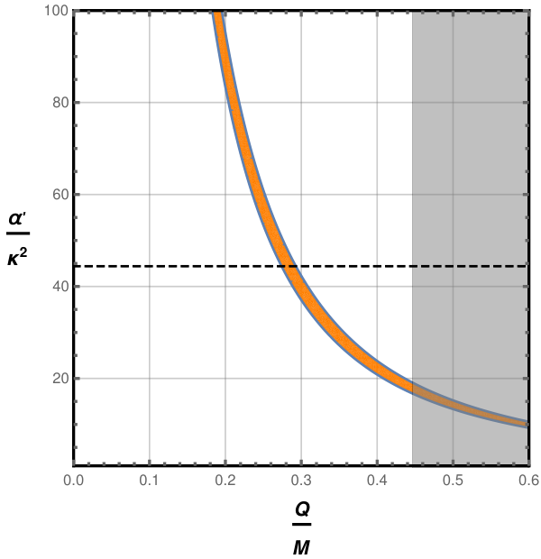
Eq.(4.8) shows that the polarization of light by the axion hair of the KSBH is dependent on the inverse string tension $\alpha^{\prime}$. Assuming that the axion hair is the only source of polarization, we show the behaviour of $\alpha^{\prime}$ with the charge of the KSBH in Fig. 4. We use the average, $30.25\pm 2.02$, of the four polarization angles in Table 1 in our estimation of $\alpha^{\prime}$. The $U(1)$ gauge kinetic term in Eq. (4.1) comes with a pre-factor of $\alpha^{\prime}/(16\kappa^{2})$ (having taken $e^{-\phi}\simeq 1$) that can be identified with $1/(4g^{2})$ where $g$ is the gauge coupling strength [57, 58, 59]. For the photon, this is just the electric charge $e$. Using this, we have:

$$\frac{\alpha^{\prime}}{16\kappa^{2}}=\frac{1}{4e^{2}}$$

(4.9)

This corresponds to the horizontal line in Fig. 4 from where we can extract the value of electric charge present in the black hole.

In this work, we studied the features of the KSBH in light of the recent M87* black hole observations from EHT and studies of polarization of light coming from near the black hole. The KSBH is a rotating charged black hole solution arising from string theory. As reported by the EHT, the black hole shadow at an inclination angle of $17^{0}$ is not completely circular with an experimental upper bound of $10\%$ on the deviation from circularity, $\Delta C$. Kerr black holes arising from general relativity cast highly circular shadows irrespective of the inclination angle leaving room for the M87* to be a non-Kerr black hole. We calculated the $\Delta C$ of the KSBH shadow using the observed M87* parameters from EHT in Sec. 3. We also found the rotation angle of the polarization of the circularly polarized light, $\Delta\Theta$, due to the axion hair of the KSBH in Sec. 4. Identifying the inverse string tension $\alpha^{\prime}$ in terms of the electromagnetic coupling strength $e$ in the relation for $\Delta\Theta$ gives us the charge of the KSBH which can then be used to predict the $\Delta C$ of the KSBH shadow in a future precision experiment. Simultaneous observation of a constant $\Delta\Theta$ (independent of the frequency of light) and $\Delta C$ for a particular value of the spin of the black hole, its inclination angle, its mass and charge could be a signature of the KSBH and thus indirectly of the string theory. We give the expected values of $\Delta\Theta$ and $\Delta C$ for some benchmark values of the KSBH charge and its inclination angle in Table 2 for a BH spin of $a/M=0.5$. As can be seen from the table, for values of the inclination angle other than $90^{0}$, ($\theta\neq 90^{0}$), it’s possible to make simultaneous observations of $\Delta\Theta$ and $\Delta C$ allowing the BH to be identified as a Kerr-Sen black hole.

There are three distinct features which can distinguish KSBH from a generic Kerr-Newman BH with axion hair:

• •

  Although the charge of the KSBH is electric in nature it is sourced by the axion-photon coupling instead of the in-falling charged particles, such as electrons or positions as in the case of charged astrophysical BH like the KNBH.

• •

  Owing to a different origin of charge, the KSBH can hold more of it than a KNBH. $Q/M$ for KSBH can be upto 1.4 whereas for KNBH, it cannot exceed 1.

• •

  In the KSBH, $\Delta\Theta$ and $\Delta C$ are correlated and the measurement of one yields the value of the other whereas in the KNBH these are independent observables.

Future, more precise, observations may be able to verify if a string solution exists in nature in the form of a Kerr-Sen black hole.

References

- [1] B. P. Abbott et al. Observation of Gravitational Waves from a Binary Black Hole Merger. Phys. Rev. Lett., 116(6):061102, 2016.
- [2] B. P. Abbott et al. GWTC-1: A Gravitational-Wave Transient Catalog of Compact Binary Mergers Observed by LIGO and Virgo during the First and Second Observing Runs. Phys. Rev., X9(3):031040, 2019.
- [3] Kazunori Akiyama et al. First M87 Event Horizon Telescope Results. I. The Shadow of the Supermassive Black Hole. Astrophys. J., 875(1):L1, 2019.
- [4] Kazunori Akiyama et al. First M87 Event Horizon Telescope Results. VI. The Shadow and Mass of the Central Black Hole. Astrophys. J., 875(1):L6, 2019.
- [5] Kazunori Akiyama et al. First M87 Event Horizon Telescope Results. V. Physical Origin of the Asymmetric Ring. Astrophys. J., 875(1):L5, 2019.
- [6] Kazunori Akiyama et al. First M87 Event Horizon Telescope Results. IV. Imaging the Central Supermassive Black Hole. Astrophys. J., 875(1):L4, 2019.
- [7] Kazunori Akiyama et al. First M87 Event Horizon Telescope Results. II. Array and Instrumentation. Astrophys. J., 875(1):L2, 2019.
- [8] Kazunori Akiyama et al. First M87 Event Horizon Telescope Results. III. Data Processing and Calibration. Astrophys. J., 875(1):L3, 2019.
- [9] Tim Johannsen and Dimitrios Psaltis. Testing the No-Hair Theorem with Observations in the Electromagnetic Spectrum: II. Black-Hole Images. Astrophys. J., 718:446–454, 2010.
- [10] Indrani Banerjee, Sumanta Chakraborty, and Soumitra SenGupta. Silhouette of M87*: A New Window to Peek into the World of Hidden Dimensions. Phys. Rev., D101(4):041301, 2020.
- [11] Vyacheslav I. Dokuchaev and Natalia O. Nazarova. Silhouettes of invisible black holes. 2019.
- [12] S. O. Alexeyev and V. A. Prokopov. Shadows from spinning black holes in extended gravity. 2020.
- [13] Rahul Kumar, Sushant G. Ghosh, and Anzhong Wang. Light Deflection and Shadow Cast by Rotating Kalb-Ramond Black Holes. 2020.
- [14] C. Y. Kuo et al. Measuring Mass Accretion Rate onto the Supermassive Black Hole in M87 Using Faraday Rotation Measure with the Submillimeter Array. Astrophys. J., 783:L33, 2014.
- [15] Frazer N. Owen, Jean A. Eilek, and William C. Keel. Detection of Large Faraday Rotation in the Inner 2 Kiloparsecs of M87. apj, 362:449, Oct 1990.
- [16] Juan-Carlos Algaba, Keiichi Asada, and Masanori Nakamura. Resolving the Rotation Measure of the m87 jet on Kiloparsec Scales. Astrophys. J., 823(2):86, 2016.
- [17] W. Junor, J. A. Biretta, and J. F. C. Wardle. VLBA lambda lambda 6, 4 cm polarimetry of Vir A. In R. T. Schilizzi, editor, Galaxies and their Constituents at the Highest Angular Resolutions, volume 205 of IAU Symposium, page 136, Jan 2001.
- [18] R. T. Zavala and G. B. Taylor. Faraday rotation measures in the parsec-scale jets of the radio galaxies m87, 3c 111, and 3c 120. Astrophys. J., 566:L9, 2002.
- [19] Yifan Chen, Jing Shu, Xiao Xue, Qiang Yuan, and Yue Zhao. Probing Axions with Event Horizon Telescope Polarimetric Measurements. Phys. Rev. Lett., 124(6):061102, 2020.
- [20] Ashoke Sen. Rotating charged black hole solution in heterotic string theory. Phys. Rev. Lett., 69:1006–1009, 1992.
- [21] Frank Wilczek. Two Applications of Axion Electrodynamics. Phys. Rev. Lett., 58:1799, 1987.
- [22] Sean M. Carroll, George B. Field, and Roman Jackiw. Limits on a Lorentz and Parity Violating Modification of Electrodynamics. Phys. Rev., D41:1231, 1990.
- [23] Sean M. Carroll and George B. Field. The Einstein equivalence principle and the polarization of radio galaxies. Phys. Rev., D43:3789, 1991.
- [24] Diego Harari and Pierre Sikivie. Effects of a Nambu-Goldstone boson on the polarization of radio galaxies and the cosmic microwave background. Phys. Lett., B289:67–72, 1992.
- [25] Galin N. Gyulchev and Stoytcho S. Yazadjiev. Kerr-Sen dilaton-axion black hole lensing in the strong deflection limit. Phys. Rev., D75:023006, 2007.
- [26] Rashmi Uniyal, Hemwati Nandan, and Philippe Jetzer. Bending angle of light in equatorial plane of Kerr–Sen Black Hole. Phys. Lett., B782:185–192, 2018.
- [27] Kenta Hioki and Umpei Miyamoto. Hidden symmetries, null geodesics, and photon capture in the Sen black hole. Phys. Rev., D78:044007, 2008.
- [28] Rashmi Uniyal, Hemwati Nandan, and K. D. Purohit. Null geodesics and observables around the Kerr–Sen black hole. Class. Quant. Grav., 35(2):025003, 2018.
- [29] Bruce A. Campbell, Nemanja Kaloper, Richard Madden, and Keith A. Olive. Physical properties of four-dimensional superstring gravity black hole solutions. Nucl. Phys., B399:137–168, 1993.
- [30] S. Ferrara, Joel Scherk, and B. Zumino. Algebraic Properties of Extended Supergravity Theories. Nucl. Phys., B121:393–402, 1977.
- [31] E. Cremmer, Joel Scherk, and S. Ferrara. U(n) Invariance in Extended Supergravity. Phys. Lett., 68B:234–238, 1977.
- [32] E. Cremmer, Joel Scherk, and S. Ferrara. SU(4) Invariant Supergravity Theory. Phys. Lett., 74B:61–64, 1978.
- [33] E. Cremmer and Joel Scherk. Algebraic Simplifications in Supergravity Theories. Nucl. Phys., B127:259–268, 1977.
- [34] E. Cremmer and B. Julia. The SO(8) Supergravity. Nucl. Phys., B159:141–212, 1979.
- [35] M. de Roo. GAUGED N=4 MATTER COUPLINGS. Phys. Lett., 156B:331–334, 1985.
- [36] L. Castellani, Anna Ceresole, S. Ferrara, R. D’Auria, P. Fre, and E. Maina. The Complete Matter Coupled Supergravity. Nucl. Phys., B268:317–348, 1986.
- [37] L. Castellani, Anna Ceresole, R. D’Auria, S. Ferrara, P. Fre, and E. Maina. Models, Duality Transformations and Scalar Potentials in Extended Supergravities. Phys. Lett., 161B:91, 1985. [,91(1985)].
- [38] S. Cecotti, S. Ferrara, and L. Girardello. Hidden Noncompact Symmetries in String Theory. Nucl. Phys., B308:436–450, 1988.
- [39] G. Veneziano. Scale factor duality for classical and quantum strings. Phys. Lett., B265:287–294, 1991.
- [40] M. J. Duff. Duality Rotations in String Theory. Nucl. Phys., B335:610, 1990.
- [41] K. A. Meissner and G. Veneziano. Symmetries of cosmological superstring vacua. Phys. Lett., B267:33–36, 1991.
- [42] K. A. Meissner and G. Veneziano. Manifestly O(d,d) invariant approach to space-time dependent string vacua. Mod. Phys. Lett., A6:3397–3404, 1991.
- [43] M. Gasperini, J. Maharana, and G. Veneziano. From trivial to nontrivial conformal string backgrounds via O(d,d) transformations. Phys. Lett., B272:277–284, 1991.
- [44] Ashoke Sen. O(d) x O(d) symmetry of the space of cosmological solutions in string theory, scale factor duality and two-dimensional black holes. Phys. Lett., B271:295–300, 1991.
- [45] James H. Horne, Gary T. Horowitz, and Alan R. Steif. An Equivalence between momentum and charge in string theory. Phys. Rev. Lett., 68:568–571, 1992.
- [46] Roy P. Kerr. Gravitational field of a spinning mass as an example of algebraically special metrics. Phys. Rev. Lett., 11:237–238, 1963.
- [47] A de Vries. The apparent shape of a rotating charged black hole, closed photon orbits and the bifurcation setA4. Classical and Quantum Gravity, 17(1):123–144, dec 1999.
- [48] A.F. Zakharov, A.A. Nucita, F. DePaolis, and G. Ingrosso. Measuring the black hole parameters in the galactic center with radioastron. New Astronomy, 10(6):479 – 489, 2005.
- [49] Zakharov, A. F., De Paolis, F., Ingrosso, G., and Nucita, A. A. Direct measurements of black hole charge with future astrometrical missions. A&A, 442(3):795–799, 2005.
- [50] Robert H. Boyer and Richard W. Lindquist. Maximal analytic extension of the kerr metric. Journal of Mathematical Physics, 8(2):265–281, 1967.
- [51] Brandon Carter. Global structure of the Kerr family of gravitational fields. Phys. Rev., 174:1559–1571, 1968.
- [52] Paul A. Blaga and Cristina Blaga. Bounded radial geodesics around a Kerr-Sen black hole. Class. Quant. Grav., 18:3893–3905, 2001.
- [53] Peter J. Young. Capture of particles from plunge orbits by a black hole. Phys. Rev., D14:3281–3289, 1976.
- [54] Cisco Gooding and Andrei V. Frolov. Five-Dimensional Black Hole Capture Cross-Sections. Phys. Rev., D77:104026, 2008.
- [55] Cosimo Bambi, Katherine Freese, Sunny Vagnozzi, and Luca Visinelli. Testing the rotational nature of the supermassive object M87* from the circularity and size of its first image. Phys. Rev., D100(4):044057, 2019.
- [56] O. Yu. Tsupko. Analytical calculation of black hole spin using deformation of the shadow. Phys. Rev., D95(10):104058, 2017.
- [57] J. Polchinski. String theory. Vol. 1: An introduction to the bosonic string. Cambridge Monographs on Mathematical Physics. Cambridge University Press, 2007.
- [58] Michael B. Green, John H. Schwarz, and Edward Witten. Superstring Theory Vol. 2. Cambridge Monographs on Mathematical Physics. Cambridge University Press, 2012.
- [59] Angel Uranga. String theory phenomenology. J. Phys. Conf. Ser., 259:012014, 2010.