跳到论文正文
W Papers独立论文阅读器 arXiv:2002.12752 论文正文 计算阅读时间 · 0%
引用这篇论文根据当前论文元数据生成,正式投稿前建议核对。


License: arXiv.org perpetual non-exclusive license
arXiv:2002.12752v1 [physics.gen-ph] 20 Feb 2020

Planck-scale effect through a new MDR

Sohan Kumar Jha Affiliation: Chandernagore College, Chandernagore, Hooghly, West Bengal, India    Himangshu Barman, Anisur Rahaman Email: anisur.rahman@saha.ac.in; manisurn@gmail.com (Corresponding Author) Affiliation: Hooghly Mohsin College, Chinsurah, Hooghly - 712101, West Bengal, India
August 11, 2026
Abstract

Abstract

In order to the expected Planck-scale correction in the physical systems we have put forwarded a novel modified dispersion relation (MDR). It has a generalized structure. A specific choice of the function used in the construction of this MDR, it has Lorentz invariance. A toy model like relativistic harmonic oscillator has been studied to get the necessary Planck-scale correction. It has been found that each laves of harmonic oscillator acquires Planck-scale correction and the result agrees with negligible deviation with the result obtained for this system for the same purpose using generalized uncertainty relation (GUP). The relativistic Hydrogen atom problem has also been studied with this MDR and it is found that like harmonic oscillator each energy level of the Hydrogen atom too has got Planck-scale correction.

I Introduction

The study of probable scenario of different physical systems in the vicinity of Planck-scale is of huge interest since the strength of the gravitational interaction in that scale becomes comparable to the strength of the electromagnetic interaction. So, in the vicinity of Planck-scale, it necessities to take into account the effect of (quantum) gravity . But straightforward quantization of gravity and its direct insertion into the physical systems is still lying at far reaching stage. Therefore, the indirect way of including the quantum gravity effect has been receiving much attention over the years through the use of novel ideas like generalized Heisenberg uncertainty principle and modified dispersion relation (MDR), as these two important ideas have been playing remarkable role towards providing necessary Planck-scale corrections into the physical systems in indirect manner GROSS; DAMIT; TYO; KKON; CRO; DOGL; PERE; ASHTE; KEMPF; SUN. This issue in the context of black body radiation was fond to be addressed in the articles MAN; NIEM; LUB; SDAS. To make statistical mechanics compatible to incorporate quantum gravity effect, formal development of it along with few applications in the thermodynamical systems have been explored in the articles SAH0; FIT; PPSM; PP0; PP1. Some experimental result also have been found to be reported to explain with the use of this type of generalization (modification)AMELI; AMELI1.

In the articles MAN; NIEM; LUB; SDAS; SAH0; FIT; PP0; PP1; PP2; KIM; ALI; HOMA; HOMA1 the concept of GUP have been exercised extensively to incorporate Planck-scale effect into different physical systems and the concept of MDR has been extended for the same purpose in the articles NOZMDR; BARUNMDR; ALIMDR; NOZMDR1; LINGMDR; SDASMDR; PPMDR. Although these two novel concepts (GUP and MDR) have been exercised in independent manner to serve essentially the same purpose in different physical systems, it is not difficult to understand conceptually that MDR and GUP are complementary to each other, however it is fair to admit that there is no established direct one to one correspondence between these two in general. It depends on the choice of generalization of the uncertainty relation or on the choice of modification of the dispersion relation. We should mention at this stage that an attempt to establish the conceptual connection between GUP and MDR is carried out recently in the article HFELD. There is indeed a special instance where a precise MDR has been proposed for a specific GUP BRM.

Although these two substantial as well as potentially effective ideas got strong initial support from string theory DAMIT; KKON; PKSTRING; MTSTRING; MAGSTRING; MAGSTRING1; LJSTRING, these two ideas were also supported immensely by the other quantum gravity candidates like loop quantum gravity ASHTE; NOZLOOP and space-time non-commutativity AR; AR1; ASU; KNOZ. In these two modifications (though in principle should considered to be merged into one) Lorentz symmetry was needed to be ignored and that necessarily led to open up a new idea namely deformed special relativity (DSR) SANG. So a natural question may arise whether this modification can be made maintaining Lorentz symmetry. It is true that there are some experimental signature which was explained inviting the Lorentz violation in an essential way GACNS, but it would be nicer indeed if it could be explained maintaining the Lorentz symmetry since violation of Lorentz symmetry invites unwanted problems to a great extent because this symmetry is deeply rooted both in field theory as well as in the general theory of relativity. The articles GAC; GAC1; GAC2 also shows a possibility of framing MDR in a Lorentz symmetric manner where deformation of d′d^{\prime} Alembertian has been exercised. In this article, we, therefore, introduce a generalized modified dispersion relation in such a way that it can be used in Lorentz invariant manner as well as with out maintaining that invariance. In this context, we should mention that in the articles VEG1; VEG2, relativistic quantum mechanical systems without quantum gravity correction have been studied and at the same time the important article VEG, is of worth mentionable where possibility of incorporating invariant quantum gravity effect at the vicinity of Planck-scale has been discussed in detail.

So it would be beneficial to designed a generalized MDR in such a fashion so that it can meet both the purpose: Lorentz invariance as well as Lorentz non-invariance extension of any physical system towards incorporating the Planck-scale effect of any physical system. With the MDR proposed here we have studied the toy model like relativistic one dimensional harmonic oscillator and a three dimensional physical system like relativistic Hydrogen atom to include the Planck-scale correction into their energy spectrum. Recently, these two systems has been studied in PSR1; PSR2 for the same purpose with the use of GUP.

The article is organized in the following manner. In Sec. I, we introduce a new generalized dispersion relation. Sec. II is devoted to get the Planck-scale correction of relativistic harmonic oscillator using rasing and lowering operator. We have shown in Sec III that the same correction can be obtained if we use differential form of momentum operator. Sec. IV contains a discussion of obtaining Planck-scale correction of the relativistic Hydrogen atom directly from the Schro¨\ddot{o}dinger’s equation. In Sec. V, the correction is computed using the average value of different powers of momentum. Sec. VI contains a brief discussion and conclusion.

II Formulation of new dispersion relation to get the Planck-scale correctiom

The generalized MDR which we are going to formulate in order to incorporate quantum gravity effect can be casted in Lorentz invariant as well as Lorentz non-invariant manner. So if the extension with this MDR is carried in a Lorentz symmetric manner one need not be worried about the search of precise DSR corresponding to this MDR. The explicit expression of this generalized MDR is

𝐏μ​𝐏μ=m02+∑kfk​(p2−E2)k.{\bf P}^{\mu}{\bf P}_{\mu}=m_{0}^{2}+\sum_{k}f_{k}(p^{2}-E^{2})^{k}. (1)

Here fk=αk(mP)k​g​(pE)f_{k}=\frac{\alpha_{k}}{(m_{P})^{k}}g(\frac{p}{E}). In general, any Lorentz non-covariant structure of the function g⁡(pE)g(\frac{p}{E}) breaks the Lorentz symmetry. However any pp independent or Lorentz covariant structure of g⁡(pE)g(\frac{p}{E}) preserves Lorentz invariance. So this new generalized MDR can be used in any physical system to incorporate Planck-scale correction in significant manner. We have chosen the simplest possible Lorentz covariant structure of the function g⁡(pE)g(\frac{p}{E}) , as g⁡(pE)=1g(\frac{p}{E})=1, which makes fk=αk(mP)kf_{k}=\frac{\alpha_{k}}{(m_{P})^{k}}. So the MDR with which we will start our investigation is

𝐏μ​𝐏μ=m02+∑kαk(mP)k​(𝐏μ​𝐏μ)k.{\bf P}^{\mu}{\bf P}_{\mu}=m_{0}^{2}+\sum_{k}\frac{\alpha_{k}}{(m_{P})^{k}}({\bf P}^{\mu}{\bf P}_{\mu})^{k}. (2)

Here m0m_{0} is the rest mass of the particle considered for study, kk is an integer that runs from k = 2 to any desired order N, P=(E,p→)P=(E,\vec{p}) and p=|p→|p=|\vec{p}|. The parameter αk\alpha_{k} represents arbitrary N-2 number of free parameters which can be fixed comparing the result obtained using this MDR with the experimental result or with the results obtained earlier through other reliable concept like GUP. The Planck-mass is characterized by the symbol mpm_{p} which is given by mP=ℏ​cGm_{P}=\sqrt{\frac{\hbar c}{G}}. Note that, reparametrization invariance in the action of a system can be maintained with this MDR (2) having manifestly lorentz covariance, since under p→−pp\rightarrow-p this MDR remains unchanged. Of course, we can define (2) in terms of Planck-length lPl_{P} in the following way

𝐏μ​𝐏μ=m02+∑kηk​(lP)k​(𝐏μ​𝐏μ)k,{\bf P}^{\mu}{\bf P}_{\mu}=m_{0}^{2}+\sum_{k}\eta_{k}(l_{P})^{k}({\bf P}^{\mu}{\bf P}_{\mu})^{k}, (3)

where ηk\eta_{k} represents N−2N-2 number of parameters certainly different from αk{\alpha_{k}} and the Planck-length lP=ℏG​c3l_{P}=\sqrt{\frac{\hbar}{Gc^{3}}}. In general, there are infinite number of parameters and numerical computation is possible with an arbitrary large numbers of such parameters, although analytical calculation will not always be possible with a desired numbers of terms. In practice however we need not keep all these parameter to get the desired accuracy.

The symbol cc stands for velocity of light in vacuum in both the cases. We will choose natural unit ℏ=1\hbar=1 and c=1c=1. To carry out our analytical investigations on relativistic harmonic oscillator and Hydrogen atom with this generalized MDR we will kept ourselves limited to k=2k=2. In due course, we will find that with the terms available for the the choice k=2k=2, the analytical computation towards Planck-scale correction for the said systems is tractable and it has good agreement with the result of the system studied earlier using the concept of GUP to incorporate the Planck-scale effect KEMPF. The MDR with k=2k=2 reads

E2=p2+m02+α2(mP)2​(p2−E2)2.E^{2}=p^{2}+m_{0}^{2}+\frac{\alpha_{2}}{(m_{P})^{2}}(p^{2}-E^{2})^{2}. (4)

A careful look reveals that this MDR resembles the deformation of the d′d^{\prime} Alembertian (□)=∂μ∂μ(\Box)=\partial_{\mu}\partial^{\mu} as it has been found in GAC; GAC1; GAC2. To be more precise: to include the dynamics of a physical system for any energy scale the deformed d′d^{\prime} Alembertian would be some desired function of the usual d′d^{\prime} Alembertian (f⁡(□))(f(\Box)) having some constants that has to be fixed with the experimental result. So to get Plank-scale effect it is to be considered that the dynamics below the Plank scale will be governed with the usual d′d^{\prime} Alembertian and the dynamics in the vicinity will be governed by the usual d′d^{\prime} Alembertian along with deformation part of the d′d^{\prime} Alembertian in a judicious manner to get necessary agreement with the experimental result (if or when available). Since both the has bears the Lorentz symmetry the frame independence of the physical result will be protected. Of course velocity of light will remain as an invariant quantity.

The hitherto available literatures related MDR show that the MDRs contain the expression of EE as a function of PP. This new MDR is not an exception to that, but it is true that the nature of the function is little generalized. The modification which is made here is only the enforcement of a physical symmetry which is none other than the celebrated Lorentz invariance which was not there in the MDR designed earlier. We have kept this point of view that in the vicinity of the Planck-scale violation of Lorentz invariance may occur but it can not be a basic criteria. On the other hand it would be admitted from all corners that Lorentz covariant structure is advantageous over Lorentz non-covariance in many respect because the basic foundation of quantum field theory and general theory of relativity is deeply rooted to the Poincar’e symmetry. The article SMO is an excellent example in this direction Therefore, this new MDR will certainly add new light in the formal development of MDR related theories. The novelty of this MDR is the welcome entry of the Lorentz symmetry and its capability to render Planck-scale correction in a frame independent manner which is lacking in the construction of MDR in the available literature dealing with Planck-scale correction with MDR.

Taking the square root of the above expression we get

E=p2+m02+α2(mP)2​(p2−E2)2.E=\sqrt{p^{2}+m_{0}^{2}+\frac{\alpha_{2}}{(m_{P})^{2}}(p^{2}-E^{2})^{2}}. (5)

Equation (5) on binomial expansion results

E\displaystyle E =\displaystyle= p22​m0+m0+α2​En42​m0​(mP)2−p2​(α2​En44​m03​(mP)2+α2​En2m0​(mP)2)\displaystyle\frac{p^{2}}{2m_{0}}+m_{0}+\frac{\alpha_{2}E_{n}^{4}}{2m_{0}(m_{P})^{2}}-p^{2}(\frac{\alpha_{2}E_{n}^{4}}{4m_{0}^{3}(m_{P})^{2}}+\frac{\alpha_{2}E_{n}^{2}}{m_{0}(m_{P})^{2}}) (6)
+\displaystyle+ p4​(α22​m0​(mP)2+α2​En22​m03​(mP)2−18​(m0)3+3​α2​En416​m05​(mP)2)\displaystyle p^{4}(\frac{\alpha_{2}}{2m_{0}(m_{P})^{2}}+\frac{\alpha_{2}E_{n}^{2}}{2m_{0}^{3}(m_{P})^{2}}-\frac{1}{8(m_{0})^{3}}+\frac{3\alpha_{2}E_{n}^{4}}{16m_{0}^{5}(m_{P})^{2}})
+\displaystyle+ p6​(−α24​m03​(mP)2+116​(m0)5−3​α2​En28​m05​(mP)2−5​α2​En432​m07​(mP)2).\displaystyle p^{6}(-\frac{\alpha_{2}}{4m_{0}^{3}(m_{P})^{2}}+\frac{1}{16(m_{0})^{5}}-\frac{3\alpha_{2}E_{n}^{2}}{8m_{0}^{5}(m_{P})^{2}}-\frac{5\alpha_{2}E_{n}^{4}}{32m_{0}^{7}(m_{P})^{2}}).

In the above expansion we have neglected terms containing higher order in α2\alpha_{2} and retained the terms up to sixth order in p. Thus our modified Hamiltonian with this settings reads

H\displaystyle H =\displaystyle= p22​m0+V+m0+α​En42​m0​(mP)2−p2​(α​En44​m03​(mP)2+α​En2m0​(mP)2)\displaystyle\frac{p^{2}}{2m_{0}}+V+m_{0}+\frac{\alpha E_{n}^{4}}{2m_{0}(m_{P})^{2}}-p^{2}(\frac{\alpha E_{n}^{4}}{4m_{0}^{3}(m_{P})^{2}}+\frac{\alpha E_{n}^{2}}{m_{0}(m_{P})^{2}}) (7)
+\displaystyle+ p4​(α2​m0​(mP)2+α​En22​m03​(mP)2−18​(m0)3+3​α​En416​m05​(mP)2)\displaystyle p^{4}(\frac{\alpha}{2m_{0}(m_{P})^{2}}+\frac{\alpha E_{n}^{2}}{2m_{0}^{3}(m_{P})^{2}}-\frac{1}{8(m_{0})^{3}}+\frac{3\alpha E_{n}^{4}}{16m_{0}^{5}(m_{P})^{2}})
+\displaystyle+ p6​(−α4​m03​(mP)2+116​(m0)5−3​α​En28​m05​(mP)2−5​α​En432​m07​(mP)2).\displaystyle p^{6}(-\frac{\alpha}{4m_{0}^{3}(m_{P})^{2}}+\frac{1}{16(m_{0})^{5}}-\frac{3\alpha E_{n}^{2}}{8m_{0}^{5}(m_{P})^{2}}-\frac{5\alpha E_{n}^{4}}{32m_{0}^{7}(m_{P})^{2}}).

In the above expression we have replaced α2\alpha_{2} by α\alpha since there is no other α\alpha’s in the body of the article. Here VV stands for the potential energy inserted by hand. To avoid confusion we would like to mention that [q,p]=i​ℏ[q,~p]=i\hbar and for modified position and momentum pair (qm,pm)(q_{m},~p_{m}) the canonical Poission’s bracket will take a modified form and that will lead to a modified uncertainty relation having a generalized form [qm,pm]=i​ℏ​f​(p,E)[q_{m},~p_{m}]=i\hbar f(p,E). The precise form of the function f⁡(p,E)f(p,E) will certainly depend on the nature of the choice of the MDR. Now using this Hamiltonian we will proceed to calculate modified eigenvalues for the relativistic harmonic oscillator and Hydrogen atom. The modified eigenvalues are in general given by

En(m)\displaystyle{E_{n}}^{(m)} =\displaystyle= En+m0+α​En42​m0​(mP)2−<p2>(α​En44​m03​(mP)2+α​En2m0​(mP)2)\displaystyle E_{n}+m_{0}+\frac{\alpha E_{n}^{4}}{2m_{0}(m_{P})^{2}}-<p^{2}>(\frac{\alpha E_{n}^{4}}{4m_{0}^{3}(m_{P})^{2}}+\frac{\alpha E_{n}^{2}}{m_{0}(m_{P})^{2}}) (8)
+\displaystyle+ <p4>(α2​m0​(mP)2+α​En22​m03​(mP)2−18​(m0)3+3​α​En416​m05​(mP)2)\displaystyle<p^{4}>(\frac{\alpha}{2m_{0}(m_{P})^{2}}+\frac{\alpha E_{n}^{2}}{2m_{0}^{3}(m_{P})^{2}}-\frac{1}{8(m_{0})^{3}}+\frac{3\alpha E_{n}^{4}}{16m_{0}^{5}(m_{P})^{2}})
+\displaystyle+ <p6>(−α4​m03​(mP)2+116​(m0)5−3​α​En28​m05​(mP)2−5​α​En432​m07​(mP)2),\displaystyle<p^{6}>(-\frac{\alpha}{4m_{0}^{3}(m_{P})^{2}}+\frac{1}{16(m_{0})^{5}}-\frac{3\alpha E_{n}^{2}}{8m_{0}^{5}(m_{P})^{2}}-\frac{5\alpha E_{n}^{4}}{32m_{0}^{7}(m_{P})^{2}}),

where En(m){E_{n}}^{(m)} and EnE_{n} are modified and unmodified eigenvalues respectively. This generalized expression shows that we have to evaluate the expectation values up to sixth power of momentum. To be precise we need the expressions of <p2><p^{2}>, <p4><p^{4}>, and <p6><p^{6}> of the system that would considered under investigation.

III Relativistic Harmonic Oscillator with MDR using raising and lowering representation of momentum operator

Let us first proceed to calculate the energy eigenvalues using raising and lowering representation of the momentum. It is known that the raising and lowering operators are respectively given by

a\displaystyle a =\displaystyle= 12​m0​ω​ℏ​(m0​ω​x+i​p),\displaystyle\frac{1}{\sqrt{2m_{0}\omega\hbar}}(m_{0}\omega x+ip), (9)
a†\displaystyle a^{\dagger} =\displaystyle= 12​m0​ω​ℏ​(m0​ω​x−i​p).\displaystyle\frac{1}{\sqrt{2m_{0}\omega\hbar}}(m_{0}\omega x-ip). (10)

For the sake of convenience we will not set ℏ=1\hbar=1 but c=1c=1 will be maintained from the starting point. However the final expression will be presented with ℏ=1\hbar=1. If aa and a+a^{+} are operated separately on the nt​hn^{th} eigen state |n>|n> we get

a|n>\displaystyle a|n> =\displaystyle= n|n−1>,\displaystyle\sqrt{n}|n-1>, (11)
a†|n>\displaystyle a^{\dagger}|n> =\displaystyle= n+1|n+1>.\displaystyle\sqrt{n+1}|n+1>. (12)

The momentum operator in terms of raising and lowering operator can be expressed as

p=i​m0​ω​ℏ2​(a†−a)p=i\sqrt{\frac{m_{0}\omega\hbar}{2}}(a^{\dagger}-a) (13)

Consecutive operation of pp on the nt​hn^{th} eigen state for two, four and six times results the following

p2|n>\displaystyle p^{2}|n> =\displaystyle= −m0​ω​ℏ2[n+1n+2|n+2>−(2n+1)|n>+nn−1|n−2>],\displaystyle-\frac{m_{0}\omega\hbar}{2}[\sqrt{n+1}\sqrt{n+2}|n+2>-(2n+1)|n>+\sqrt{n}\sqrt{n-1}|n-2>], (14)
p4|n>\displaystyle p^{4}|n> =\displaystyle= (m0​ω​ℏ2)2[n+1n+2n+3n+4|n+4>\displaystyle(\frac{m_{0}\omega\hbar}{2})^{2}[\sqrt{n+1}\sqrt{n+2}\sqrt{n+3}\sqrt{n+4}|n+4> (15)
−\displaystyle- n+1​n+2​(4​n+6)|n+2>\displaystyle\sqrt{n+1}\sqrt{n+2}(4n+6)|n+2>
+\displaystyle+ (6​n2+6​n+3)|n>−n​n−1​(4​n−2)|n−2>\displaystyle(6n^{2}+6n+3)|n>-\sqrt{n}\sqrt{n-1}(4n-2)|n-2>
+\displaystyle+ nn−1n−2n−3|n−4>],\displaystyle\sqrt{n}\sqrt{n-1}\sqrt{n-2}\sqrt{n-3}|n-4>],
p6|n>\displaystyle p^{6}|n> =\displaystyle= −(m0​ω​ℏ2)3[n+1n+2n+3n+4n+5n+6|n+6>\displaystyle-(\frac{m_{0}\omega\hbar}{2})^{3}[\sqrt{n+1}\sqrt{n+2}\sqrt{n+3}\sqrt{n+4}\sqrt{n+5}\sqrt{n+6}|n+6> (16)
−\displaystyle- n+1​n+2​n+3​n+4​(6​n+15)|n+4>\displaystyle\sqrt{n+1}\sqrt{n+2}\sqrt{n+3}\sqrt{n+4}(6n+15)|n+4>
+\displaystyle+ n+1​n+2​(15​n2+45​n+45)|n+2>\displaystyle\sqrt{n+1}\sqrt{n+2}(15n^{2}+45n+45)|n+2>
−\displaystyle- (20​n3+30​n2+40​n+15)|n>\displaystyle(20n^{3}+30n^{2}+40n+15)|n>
+\displaystyle+ n​n−1​(15​n2−15​n+15)|n−2>\displaystyle\sqrt{n}\sqrt{n-1}(15n^{2}-15n+15)|n-2>
−\displaystyle- n​n−1​n−2​n−3​(6​n−9)|n−4>\displaystyle\sqrt{n}\sqrt{n-1}\sqrt{n-2}\sqrt{n-3}(6n-9)|n-4>
+\displaystyle+ nn−1n−2n−3n−4n−5|n−6>].\displaystyle\sqrt{n}\sqrt{n-1}\sqrt{n-2}\sqrt{n-3}\sqrt{n-4}\sqrt{n-5}|n-6>].

If we now take the inner product of the above expression with |n>|n> we will get the required expectation values of p2p^{2}, p4p^{4} and p6p^{6}. The precise expression of the expectation values are

<p2>\displaystyle<p^{2}> =\displaystyle= m0​ω​ℏ2​(2​n+1),\displaystyle\frac{m_{0}\omega\hbar}{2}(2n+1), (17)
<p4>\displaystyle<p^{4}> =\displaystyle= (m0​ω​ℏ2)2​(6​n2+6​n+3),\displaystyle(\frac{m_{0}\omega\hbar}{2})^{2}(6n^{2}+6n+3), (18)
<p6>\displaystyle<p^{6}> =\displaystyle= (m0​ω​ℏ2)3​(20​n3+30​n2+40​n+15),\displaystyle(\frac{m_{0}\omega\hbar}{2})^{3}(20n^{3}+30n^{2}+40n+15), (19)

which leads us to get the modified eigenvalues with this Lorentz symmetric modified dispersion relation

En(m​h​o)\displaystyle{E_{n}}^{(mho)} =\displaystyle= En+m0+α​En42​m0​(mP)2−m0​ω​ℏ2​(2​n+1)​(α​En44​m03​(mP)2+α​En2m0​(mP)2)\displaystyle E_{n}+m_{0}+\frac{\alpha E_{n}^{4}}{2m_{0}(m_{P})^{2}}-\frac{m_{0}\omega\hbar}{2}(2n+1)(\frac{\alpha E_{n}^{4}}{4m_{0}^{3}(m_{P})^{2}}+\frac{\alpha E_{n}^{2}}{m_{0}(m_{P})^{2}}) (20)
+\displaystyle+ (m0​ω​ℏ2)2​(6​n2+6​n+3)​(α2​m0​(mP)2+α​En22​m03​(mP)2−18​(m0)3+3​α​En416​m05​(mP)2)\displaystyle(\frac{m_{0}\omega\hbar}{2})^{2}(6n^{2}+6n+3)(\frac{\alpha}{2m_{0}(m_{P})^{2}}+\frac{\alpha E_{n}^{2}}{2m_{0}^{3}(m_{P})^{2}}-\frac{1}{8(m_{0})^{3}}+\frac{3\alpha E_{n}^{4}}{16m_{0}^{5}(m_{P})^{2}})
+\displaystyle+ (m0​ω​ℏ2)3×(20​n3+30​n2+40​n+15)\displaystyle(\frac{m_{0}\omega\hbar}{2})^{3}\times(20n^{3}+30n^{2}+40n+15)
(\displaystyle( OPEN−α4​m03​(mP)2+116​(m0)5−3​α​En28​m05​(mP)2−5​α​En432​m07​(mP)2).\displaystyle-\frac{\alpha}{4m_{0}^{3}(m_{P})^{2}}+\frac{1}{16(m_{0})^{5}}-\frac{3\alpha E_{n}^{2}}{8m_{0}^{5}(m_{P})^{2}}-\frac{5\alpha E_{n}^{4}}{32m_{0}^{7}(m_{P})^{2}}).

Equation (20) reveals that each levels of hydrogen atom acquires Planck-scale correction which was also found in the articles PSR1; PSR2 where concept of GUP was employed to incorporate quantum gravity effect. This result is amenable to compare with the correction obtained in KEMPF, using the concept of GUP for incorporation of quantum gravity correction. We will now turn to calculate the modified energy eigenvalues using the differential form of the momentum to get it confirmed whether these two agrees with each other.

III.1 Calculation using differential form of momentum operator

We know that momentum operator in differential form with the coordinate representation can is written down as

p=−i​ℏ​∂∂x,i=−1,p=-i\hbar\frac{\partial}{\partial x},~~~~i=\sqrt{-1}, (21)

and the nt​hn^{th} state eigenfunction of a harmonic oscillator is known to be

ψn=aπ​2n​n!​Hn​(a​x)​e−a2​x22,a=m0​ωℏ,\psi_{n}=\sqrt{\frac{a}{\sqrt{\pi}2^{n}n!}}H_{n}(ax)e^{\frac{-a^{2}x^{2}}{2}},a=\sqrt{\frac{m_{0}\omega}{\hbar}}, (22)

where Hn​(a​x)H_{n}(ax), represents the Hermite polynomial of order n. Bringing the momentum operator in repeated action for two, four and six times and multiplying the obtained result by ψn\psi_{n} and hence integrating within the limit −∞-\infty to ∞\infty we get the expectation values of p2p^{2}, p4p^{4} and p6p^{6}:

<p2>=\displaystyle<p^{2}>= −\displaystyle- ℏ2aπ​2n​n![∫−∞∞(a4x2−a2)e−a2​x2Hn(ax)Hn(ax)dx\displaystyle\hbar^{2}\frac{a}{\sqrt{\pi}2^{n}n!}[\int_{-\infty}^{\infty}(a^{4}x^{2}-a^{2})e^{-a^{2}x^{2}}H_{n}(ax)H_{n}(ax)dx (23)
−\displaystyle- 4​n​a3​∫−∞∞x​ea2​x2​Hn−1​(a​x)​Hn​(a​x)​𝑑x\displaystyle 4na^{3}\int_{-\infty}^{\infty}xe^{a^{2}x^{2}}H_{n-1}(ax)H_{n}(ax)dx
+\displaystyle+ 4n(n−1)a2∫−∞∞ea2​x2Hn−2(ax)Hn(ax)dx]\displaystyle 4n(n-1)a^{2}\int_{-\infty}^{\infty}e^{a^{2}x^{2}}H_{n-2}(ax)H_{n}(ax)dx]
=\displaystyle= m0​ω​ℏ2​(2​n+1),\displaystyle\frac{m_{0}\omega\hbar}{2}(2n+1), (24)
<p4>=\displaystyle<p^{4}>= ℏ4aπ​2n​n![16n(n−1)(n−2)(n−3)a4∫−∞∞ea2​x2Hn−4(ax)Hn(ax)dx\displaystyle\hbar^{4}\frac{a}{\sqrt{\pi}2^{n}n!}[16n(n-1)(n-2)(n-3)a^{4}\int_{-\infty}^{\infty}e^{a^{2}x^{2}}H_{n-4}(ax)H_{n}(ax)dx (25)
−\displaystyle- 32​n​(n−1)​(n−2)​a5​∫−∞∞x​ea2​x2​Hn−3​(a​x)​Hn​(a​x)​𝑑x\displaystyle 32n(n-1)(n-2)a^{5}\int_{-\infty}^{\infty}xe^{a^{2}x^{2}}H_{n-3}(ax)H_{n}(ax)dx
+\displaystyle+ 24​n​(n−1)​∫−∞∞(a6​x2−a4)​ea2​x2​Hn−2​(a​x)​Hn​(a​x)​𝑑x\displaystyle 24n(n-1)\int_{-\infty}^{\infty}(a^{6}x^{2}-a^{4})e^{a^{2}x^{2}}H_{n-2}(ax)H_{n}(ax)dx
+\displaystyle+ ∫−∞∞(24​n​a5​x−8​n​a7​x3)​ea2​x2​Hn−1​(a​x)​Hn​(a​x)​𝑑x\displaystyle\int_{-\infty}^{\infty}(24na^{5}x-8na^{7}x^{3})e^{a^{2}x^{2}}H_{n-1}(ax)H_{n}(ax)dx
+\displaystyle+ ∫−∞∞(3a4−6a6x2+a8x4)ea2​x2Hn(ax)Hn(ax)dx]\displaystyle\int_{-\infty}^{\infty}(3a^{4}-6a^{6}x^{2}+a^{8}x^{4})e^{a^{2}x^{2}}H_{n}(ax)H_{n}(ax)dx]
=\displaystyle= (m0​ω​ℏ2)2​(6​n2+6​n+3),\displaystyle(\frac{m_{0}\omega\hbar}{2})^{2}(6n^{2}+6n+3), (26)
<p6>=\displaystyle<p^{6}>= −\displaystyle- ℏ6aπ​2n​n![64n(n−1)(n−2)(n−3)(n−4)(n−5)a6∫−∞∞ea2​x2Hn−6(ax)Hn(ax)dx\displaystyle\hbar^{6}\frac{a}{\sqrt{\pi}2^{n}n!}[64n(n-1)(n-2)(n-3)(n-4)(n-5)a^{6}\int_{-\infty}^{\infty}e^{a^{2}x^{2}}H_{n-6}(ax)H_{n}(ax)dx (27)
−\displaystyle- 192​n​(n−1)​(n−2)​(n−3)​(n−4)​a7​∫−∞∞x​ea2​x2​Hn−5​(a​x)​Hn​(a​x)​𝑑x\displaystyle 192n(n-1)(n-2)(n-3)(n-4)a^{7}\int_{-\infty}^{\infty}xe^{a^{2}x^{2}}H_{n-5}(ax)H_{n}(ax)dx
+\displaystyle+ 240​n​(n−1)​(n−2)​(n−3)​∫−∞∞(a8​x2−a6)​ea2​x2​Hn−4​(a​x)​Hn​(a​x)​𝑑x\displaystyle 240n(n-1)(n-2)(n-3)\int_{-\infty}^{\infty}(a^{8}x^{2}-a^{6})e^{a^{2}x^{2}}H_{n-4}(ax)H_{n}(ax)dx
+\displaystyle+ n⁡(n−1)​(n−2)​∫−∞∞(480​a7​x−160​a9​x3)​ea2​x2​Hn−3​(a​x)​Hn​(a​x)​𝑑x\displaystyle n(n-1)(n-2)\int_{-\infty}^{\infty}(480a^{7}x-160a^{9}x^{3})e^{a^{2}x^{2}}H_{n-3}(ax)H_{n}(ax)dx
+\displaystyle+ n⁡(n−1)​∫−∞∞(180​a6−360​a8​x2+60​a1​0​x4)​ea2​x2​Hn−2​(a​x)​Hn​(a​x)​𝑑x\displaystyle n(n-1)\int_{-\infty}^{\infty}(180a^{6}-360a^{8}x^{2}+60a^{1}0x^{4})e^{a^{2}x^{2}}H_{n-2}(ax)H_{n}(ax)dx
+\displaystyle+ n​∫−∞∞(−180​a7​x+120​a9​x3−12​a1​1​x5)​ea2​x2​Hn−1​(a​x)​Hn​(a​x)​𝑑x\displaystyle n\int_{-\infty}^{\infty}(-180a^{7}x+120a^{9}x^{3}-12a^{1}1x^{5})e^{a^{2}x^{2}}H_{n-1}(ax)H_{n}(ax)dx
+\displaystyle+ ∫−∞∞(45​a8​x2−15​a6−15​a1​0​x4+a1​2​x6)​ea2​x2​Hn​(a​x)​Hn​(a​x)​𝑑x\displaystyle\int_{-\infty}^{\infty}(45a^{8}x^{2}-15a^{6}-15a^{1}0x^{4}+a^{1}2x^{6})e^{a^{2}x^{2}}H_{n}(ax)H_{n}(ax)dx
=\displaystyle= (m0​ω​ℏ2)3​(20​n3+30​n2+40​n+15).\displaystyle(\frac{m_{0}\omega\hbar}{2})^{3}(20n^{3}+30n^{2}+40n+15). (28)

In the above computation we have used the following recurrence relations.

Hn+1​(x)=2​x​Hn​(x)−2​n​Hn−1​(x),d​Hn​(x)d​x=2​n​Hn−1​(x).\displaystyle H_{n+1}(x)=2xH_{n}(x)-2nH_{n-1}(x),~~~\frac{dH_{n}(x)}{dx}=2nH_{n-1}(x). (29)

The the standard integrals

∫−∞∞ex2​Hm​(x)​Hn​(x)​𝑑x\displaystyle\int_{-\infty}^{\infty}e^{x^{2}}H_{m}(x)H_{n}(x)dx =\displaystyle= 2n​π​n!​δm​n,\displaystyle 2^{n}\sqrt{\pi}n!\delta_{mn}, (30)
∫−∞∞x​ex2​Hm​(x)​Hn​(x)​𝑑x\displaystyle\int_{-\infty}^{\infty}xe^{x^{2}}H_{m}(x)H_{n}(x)dx =\displaystyle= 2n−1​π​n!​δm,n−1+2n​π​(n+1)!​δm,n+1,\displaystyle 2^{n-1}\sqrt{\pi}n!\delta_{m,n-1}+2^{n}\sqrt{\pi}(n+1)!\delta_{m,n+1}, (31)
∫−∞∞x2​ex2​Hm​(x)​Hn​(x)​𝑑x\displaystyle\int_{-\infty}^{\infty}x^{2}e^{x^{2}}H_{m}(x)H_{n}(x)dx =\displaystyle= 2n−2​π​n!​δm,n−2+(2​n+1)​2n−1​π​n!​δm,n+2n​π​(n+2)!​δm,n+2,\displaystyle 2^{n-2}\sqrt{\pi}n!\delta_{m,n-2}+(2n+1)2^{n-1}\sqrt{\pi}n!\delta_{m,n}+2^{n}\sqrt{\pi}(n+2)!\delta_{m,n+2}, (32)

are also needed for the required computation. Using the above recurrence relations and the standard integrals the final expression of the modified eigenvalues come out to be

En(m​h​o)\displaystyle{E_{n}}^{(mho)} =\displaystyle= En+m0+α​En42​m0​(mP)2−m0​ω​ℏ2​(2​n+1)​(α​En44​m03​(mP)2+α​En2m0​(mP)2)\displaystyle E_{n}+m_{0}+\frac{\alpha E_{n}^{4}}{2m_{0}(m_{P})^{2}}-\frac{m_{0}\omega\hbar}{2}(2n+1)(\frac{\alpha E_{n}^{4}}{4m_{0}^{3}(m_{P})^{2}}+\frac{\alpha E_{n}^{2}}{m_{0}(m_{P})^{2}}) (33)
+\displaystyle+ (m0​ω​ℏ2)2​(6​n2+6​n+3)​(α2​m0​(mP)2+α​En22​m03​(mP)2−18​(m0)3+3​α​En416​m05​(mP)2)\displaystyle(\frac{m_{0}\omega\hbar}{2})^{2}(6n^{2}+6n+3)(\frac{\alpha}{2m_{0}(m_{P})^{2}}+\frac{\alpha E_{n}^{2}}{2m_{0}^{3}(m_{P})^{2}}-\frac{1}{8(m_{0})^{3}}+\frac{3\alpha E_{n}^{4}}{16m_{0}^{5}(m_{P})^{2}})
+\displaystyle+ (m0​ω​ℏ2)3​(20​n3+30​n2+40​n+15)\displaystyle(\frac{m_{0}\omega\hbar}{2})^{3}(20n^{3}+30n^{2}+40n+15)
(−α4​m03​(mP)2+116​(m0)5−3​α​En28​m05​(mP)2−5​α​En432​m07​(mP)2).\displaystyle(-\frac{\alpha}{4m_{0}^{3}(m_{P})^{2}}+\frac{1}{16(m_{0})^{5}}-\frac{3\alpha E_{n}^{2}}{8m_{0}^{5}(m_{P})^{2}}-\frac{5\alpha E_{n}^{4}}{32m_{0}^{7}(m_{P})^{2}}).

Note that identical expression for eigenvalue En(m){E_{n}}^{(m)} has come out for both the cases: when momentum is expressed in terms of rasing and lowering operator as well as when the differential form of the momentum operator is used for computation. This is of course, the expected scenario. The expression obtained in (20) and (33) do not have Lorentz symmetric structure although the the Lorentz covariant MDR has been used for computation of eigenvalues, because we have not considered the full relativistic theory. For full relativistic Hamiltonian the result ought to be Lorentz symmetric if at all the exact analytical extension is feasible in this situation.

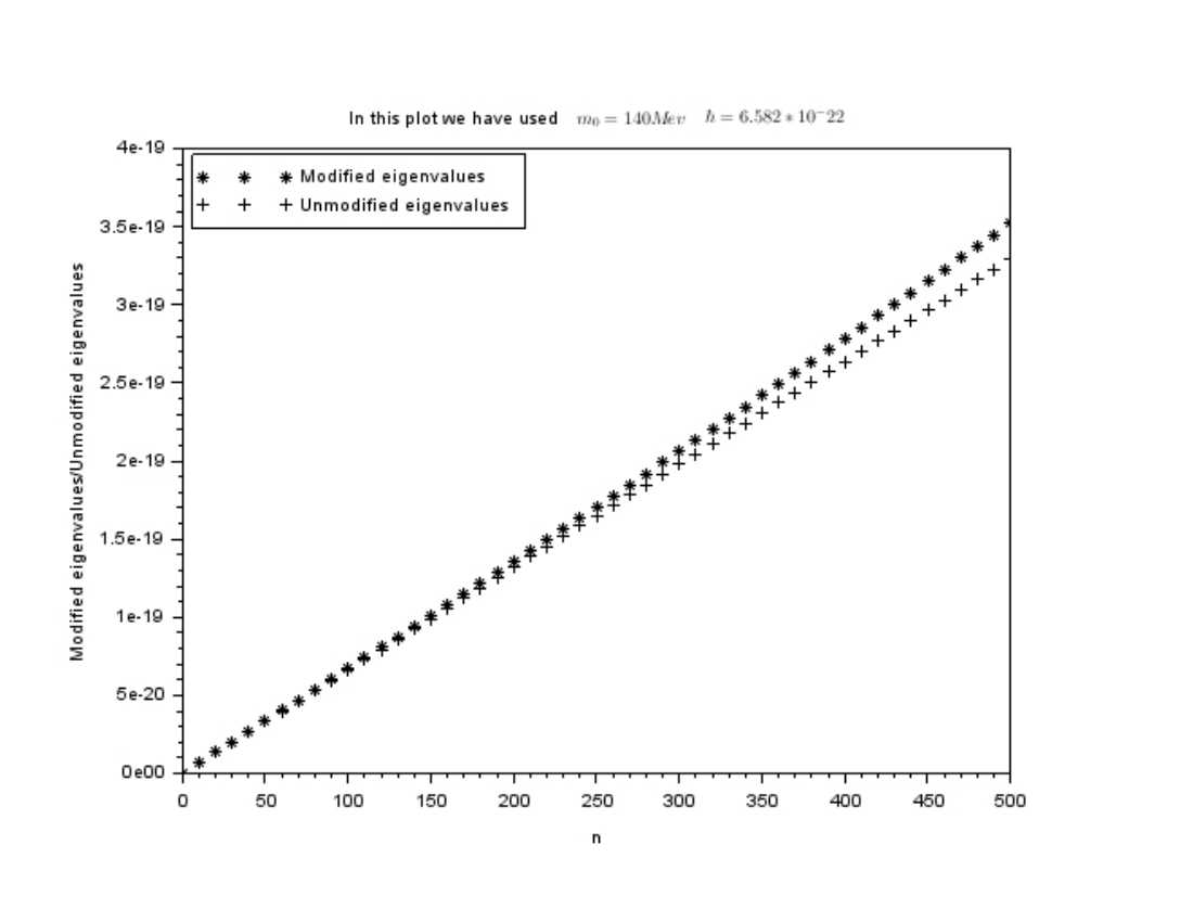
Fig.1 shows a plot of the energy eigenvalues versus nn for α=1.6×10−39\alpha=1.6\times 10^{-39}. Note that energy eigenvalues is plotted subtracting the rest mass energy from it. The spectrum agrees with spectrum obtained in the article KEMPF which was evaluated using a quadratic GUP. In our case modification is resulted with the introduction of a generalized MDR. It ravels once again that GUP and MDR essentially serve the same purpose which is indeed the obtaining the quantum gravity correction at the vicinity of Planck-scale. The agreement of our result with the result obtained in the article KEMPF is natural since the MDR and GUP basically serves the same purpose although it is fair to admit that there is no one to one correspondence between this generalized MDR used here and the GUP used in KEMPF.
Refer to caption

Figure 1: A Picture

IV Modified eigenvalues of Hydrogen atom using Schro¨\ddot{o}dinger’s equation

Let us now proceed to obtain quantum gravity correction to the spectrum of Hydrogen atom. The Schro¨\ddot{o}dinger’s equation for Hydrogen atom reads

p22​m0​ψn​l​m−e24​π​ε0​r​ψn​l​m=En​ψn​l​m,\frac{p^{2}}{2m_{0}}\psi_{nlm}-\frac{e^{2}}{4\pi\varepsilon_{0}r}\psi_{nlm}=E_{n}\psi_{nlm}, (34)

where

ψn​l​m=Rn​l​Ylm​(θ​φ)=un​lr​Ylm​(θ​φ),\psi_{nlm}=R_{nl}Y_{l}^{m}(\theta\varphi)=\frac{u_{nl}}{r}Y_{l}^{m}(\theta\varphi), (35)

This gives

p2​ψn​l​m=2​m0​[En+e24​π​ε0​r]​ψn​l​m,p^{2}\psi_{nlm}=2m_{0}[E_{n}+\frac{e^{2}}{4\pi\varepsilon_{0}r}]\psi_{nlm}, (36)

and hence the expectation value of p2p^{2} is given by

<p2>=2m0[En+e24​π​ε0<1r>].<p^{2}>=2m_{0}[E_{n}+\frac{e^{2}}{4\pi\varepsilon_{0}}<\frac{1}{r}>]. (37)

If p4p^{4} and p6p^{6} on ψn​l​m\psi_{nlm} get operated on (35) we ultimately have

p4​(ψn​l​m)\displaystyle p^{4}(\psi_{nlm}) =\displaystyle= 4​m02​En​[En+e24​π​ε0​r]​ψn​l​m+m0​e22​π​ε0​[2​ℏ2​Ylmr2​d​Rn​ld​r+2​m0r​(En+e24​π​ε0​r)​ψn​l​m],\displaystyle 4m_{0}^{2}E_{n}[E_{n}+\frac{e^{2}}{4\pi\varepsilon_{0}r}]\psi_{nlm}+\frac{m_{0}e^{2}}{2\pi\varepsilon_{0}}[\frac{2\hbar^{2}Y_{l}^{m}}{r^{2}}\frac{dR_{nl}}{dr}+\frac{2m_{0}}{r}(E_{n}+\frac{e^{2}}{4\pi\varepsilon_{0}r})\psi_{nlm}], (38)
p6​(ψn​l​m)\displaystyle p^{6}(\psi_{nlm}) =\displaystyle= 8​m03​En2​[En+e24​π​ε0​r]​ψn​l​m+2​m02​e2​Enπ​ε0​[2​ℏ2​Ylmr2​d​Rn​ld​r+(2​m0​Enr+m0​e22​π​ε0​r2)​ψn​l​m]\displaystyle 8m_{0}^{3}E_{n}^{2}[E_{n}+\frac{e^{2}}{4\pi\varepsilon_{0}r}]\psi_{nlm}+\frac{2m_{0}^{2}e^{2}E_{n}}{\pi\varepsilon_{0}}[\frac{2\hbar^{2}Y_{l}^{m}}{r^{2}}\frac{dR_{nl}}{dr}+(\frac{2m_{0}E_{n}}{r}+\frac{m_{0}e^{2}}{2\pi\varepsilon_{0}r^{2}})\psi_{nlm}] (39)
+\displaystyle+ m02​e44​π2​ε2​[(m0​e22​π​ε0​r3​2​m0​Enr2)​ψn​l​m+4​ℏ2​Ylmr4​d​un​ld​r−6​ℏ2r4​ψn​l​m]\displaystyle\frac{m_{0}^{2}e^{4}}{4\pi^{2}\varepsilon^{2}}[(\frac{m_{0}e^{2}}{2\pi\varepsilon_{0}r^{3}}\frac{2m_{0}E_{n}}{r^{2}})\psi_{nlm}+\frac{4\hbar^{2}Y_{l}^{m}}{r^{4}}\frac{du_{nl}}{dr}-\frac{6\hbar^{2}}{r^{4}}\psi_{nlm}]
+\displaystyle+ m0​e2​ℏ2π​ε0[l⁡(l+1)​ℏ2​Ylmr4d​Rn​ld​r+12​ℏ2r5ψn​l​m+(5​l​(l+1)​ℏ2r5−5​m0​e22​π​ε0​r4−10​m0​Enr3)ψn​l​m\displaystyle\frac{m_{0}e^{2}\hbar^{2}}{\pi\varepsilon_{0}}[\frac{l(l+1)\hbar^{2}Y_{l}^{m}}{r^{4}}\frac{dR_{nl}}{dr}+\frac{12\hbar^{2}}{r^{5}}\psi_{nlm}+(\frac{5l(l+1)\hbar^{2}}{r^{5}}-\frac{5m_{0}e^{2}}{2\pi\varepsilon_{0}r^{4}}-\frac{10m_{0}E_{n}}{r^{3}})\psi_{nlm}
−\displaystyle- ℏ2Ylm(1r3d3​un​ld​r3+12r5d​un​ld​r)].\displaystyle\hbar^{2}Y_{l}^{m}(\frac{1}{r^{3}}\frac{d^{3}u_{nl}}{dr^{3}}+\frac{12}{r^{5}}\frac{du_{nl}}{dr})].

These lead us to obtain the expectation value of p4p^{4}:

<p4>=4​m02​En2+2​m02​e2​Enπ​ε0<1r>+m02​e44​π2​ε02<1r2>.<p^{4}>=4m_{0}^{2}E_{n}^{2}+\frac{2m_{0}^{2}e^{2}E_{n}}{\pi\varepsilon_{0}}<\frac{1}{r}>+\frac{m_{0}^{2}e^{4}}{4\pi^{2}\varepsilon_{0}^{2}}<\frac{1}{r^{2}}>. (40)

To get the desired result we have used the stand integral

∫0∞Rn​l​d​Rn​ld​r​𝑑r=0.\int_{0}^{\infty}R_{nl}\frac{dR_{nl}}{dr}dr=0. (41)

The expectation value of p6p^{6} is now found out in a straightforward manner:

<p6>=\displaystyle<p^{6}>= 8​m03​En3+6​m03​e2​En2π​ε0<1r>+3​m03​e4​En2​π2​ε2<1r2>+[m03​e68​π3​ε03−8​m02​En​e2​ℏ2π​ε0]<1r3>\displaystyle 8m_{0}^{3}E_{n}^{3}+\frac{6m_{0}^{3}e^{2}E_{n}^{2}}{\pi\varepsilon_{0}}<\frac{1}{r}>+\frac{3m_{0}^{3}e^{4}E_{n}}{2\pi^{2}\varepsilon^{2}}<\frac{1}{r^{2}}>+[\frac{m_{0}^{3}e^{6}}{8\pi^{3}\varepsilon_{0}^{3}}-\frac{8m_{0}^{2}E_{n}e^{2}\hbar^{2}}{\pi\varepsilon_{0}}]<\frac{1}{r^{3}}> (42)
−\displaystyle- 9​m02​e4​ℏ24​π2​ε02<1r4>+m0​e2​ℏ2π​ε0​[6​l​(l+1)​ℏ2−12​ℏ2]<1r5>.\displaystyle\frac{9m_{0}^{2}e^{4}\hbar^{2}}{4\pi^{2}\varepsilon_{0}^{2}}<\frac{1}{r^{4}}>+\frac{m_{0}e^{2}\hbar^{2}}{\pi\varepsilon_{0}}[6l(l+1)\hbar^{2}-12\hbar^{2}]<\frac{1}{r^{5}}>.

To this end, Feynmann-Hellman theorem helps a lot to get the expressions of <1r><\frac{1}{r}> and <1r2><\frac{1}{r^{2}}>: Ultimately, we see that

<1r>\displaystyle<\frac{1}{r}> =\displaystyle= 1n2​a0,\displaystyle\frac{1}{n^{2}a_{0}}, (43)
<1r2>\displaystyle<\frac{1}{r^{2}}> =\displaystyle= 2n3​a02​(2​l+1),\displaystyle\frac{2}{n^{3}a_{0}^{2}(2l+1)}, (44)

where a0a_{0} is the Bohr radius. To get the exact expression of <1r3><\frac{1}{r^{3}}>,<1r4><\frac{1}{r^{4}}> and <1r5><\frac{1}{r^{5}}> Kramers’ relation GRIF also has been employed here which is given by

s+1n2<rs>−(2​s+1)​a0<rs−1>+s4​[(2​l+1)2−s2]​a02<rs−2>=0.\frac{s+1}{n^{2}}<r^{s}>-(2s+1)a_{0}<r^{s-1}>+\frac{s}{4}[(2l+1)^{2}-s^{2}]a_{0}^{2}<r^{s-2}>=0. (45)

If s=−1s=-1 is set in the Kramers’ relation it leads to obtain the expression of <1r3><\frac{1}{r^{3}}>:

<1r3>=2a03​n3​l​(l+1)​(2​l+1),<\frac{1}{r^{3}}>=\frac{2}{a_{0}^{3}n^{3}l(l+1)(2l+1)}, (46)

In a similar way it we put s=−2s=-2 in the Kramers’ relation it gives the expression of <1r4><\frac{1}{r^{4}}>

<1r4>=12a04​n3​l​(l+1)​(2​l+3)​(4​l2−1)−4a04​n5​(2​l+3)​(4​l2−1).<\frac{1}{r^{4}}>=\frac{12}{a_{0}^{4}n^{3}l(l+1)(2l+3)(4l^{2}-1)}-\frac{4}{a_{0}^{4}n^{5}(2l+3)(4l^{2}-1)}. (47)

Finally, putting s=−3s=-3 we get the expression of <1r5><\frac{1}{r^{5}}>:

<1r5>=\displaystyle<\frac{1}{r^{5}}>= 20a05​n3​l​(l2−1)​(l+2)​(2​l+3)​(4​l2−1)\displaystyle\frac{20}{a_{0}^{5}n^{3}l(l^{2}-1)(l+2)(2l+3)(4l^{2}-1)} (48)
−\displaystyle- 203​a05​n5​(l−1)​(l+2)​(2​l+3)​(4​l2−1)\displaystyle\frac{20}{3a_{0}^{5}n^{5}(l-1)(l+2)(2l+3)(4l^{2}-1)}
−\displaystyle- 43​a05​n5​l​(l2−1)​(l+2)​(2​l+1).\displaystyle\frac{4}{3a_{0}^{5}n^{5}l(l^{2}-1)(l+2)(2l+1)}.

Substituting these in the expression for <p2><p^{2}>, <p4><p^{4}> and <p6><p^{6}> we land on to the following.

<p2>\displaystyle<p^{2}> =\displaystyle= 2​m0​[En+ℏ2m0​a02​n2],\displaystyle 2m_{0}[E_{n}+\frac{\hbar^{2}}{m_{0}a_{0}^{2}n^{2}}], (49)
<p4>\displaystyle<p^{4}> =\displaystyle= 8​ℏ4a04​n3​(2​l+1)+4​m02​En2+8​m0​En​ℏ2n2​a02,\displaystyle\frac{8\hbar^{4}}{a_{0}^{4}n^{3}(2l+1)}+4m_{0}^{2}E_{n}^{2}+\frac{8m_{0}E_{n}\hbar^{2}}{n^{2}a_{0}^{2}}, (50)
<p6>\displaystyle<p^{6}> =\displaystyle= 8​m03​En3+6​m03​e2​En2π​ε0​1n2​a0\displaystyle 8m_{0}^{3}E_{n}^{3}+\frac{6m_{0}^{3}e^{2}E_{n}^{2}}{\pi\varepsilon_{0}}\frac{1}{n^{2}a_{0}} (51)
+\displaystyle+ 3​m03​e4​En2​π2​ε2​2n3​a02​(2​l+1)+[m03​e68​π3​ε03−8​m02​En​e2​ℏ2π​ε0]​2a03​n3​l​(l+1)​(2​l+1)\displaystyle\frac{3m_{0}^{3}e^{4}E_{n}}{2\pi^{2}\varepsilon^{2}}\frac{2}{n^{3}a_{0}^{2}(2l+1)}+[\frac{m_{0}^{3}e^{6}}{8\pi^{3}\varepsilon_{0}^{3}}-\frac{8m_{0}^{2}E_{n}e^{2}\hbar^{2}}{\pi\varepsilon_{0}}]\frac{2}{a_{0}^{3}n^{3}l(l+1)(2l+1)}
−\displaystyle- 9​m02​e4​ℏ24​π2​ε02​[12a04​n3​l​(l+1)​(2​l+3)​(4​l2−1)−4a04​n5​(2​l+3)​(4​l2−1)]\displaystyle\frac{9m_{0}^{2}e^{4}\hbar^{2}}{4\pi^{2}\varepsilon_{0}^{2}}[\frac{12}{a_{0}^{4}n^{3}l(l+1)(2l+3)(4l^{2}-1)}-\frac{4}{a_{0}^{4}n^{5}(2l+3)(4l^{2}-1)}]
+\displaystyle+ m0​e2​ℏ2π​ε0[6l(l+1)ℏ2−12ℏ2][20a05​n3​l​(l2−1)​(l+2)​(2​l+3)​(4​l2−1)\displaystyle\frac{m_{0}e^{2}\hbar^{2}}{\pi\varepsilon_{0}}[6l(l+1)\hbar^{2}-12\hbar^{2}][\frac{20}{a_{0}^{5}n^{3}l(l^{2}-1)(l+2)(2l+3)(4l^{2}-1)}
−\displaystyle- 203​a05​n5​(l−1)​(l+2)​(2​l+3)​(4​l2−1)−43​a05​n5​l​(l2−1)​(l+2)​(2​l+1)].\displaystyle\frac{20}{3a_{0}^{5}n^{5}(l-1)(l+2)(2l+3)(4l^{2}-1)}-\frac{4}{3a_{0}^{5}n^{5}l(l^{2}-1)(l+2)(2l+1)}].

Thus the modified eigenvalues for Hydrogen atom finally come out as

En(m​h​a)=\displaystyle{E_{n}}^{(mha)}= En+m0+α​En42​m0​(mP)2−2​m0​[En+ℏ2m0​a02​n2]​(α​En44​m03​(mP)2+α​En2m0​(mP)2)\displaystyle E_{n}+m_{0}+\frac{\alpha E_{n}^{4}}{2m_{0}(m_{P})^{2}}-2m_{0}[E_{n}+\frac{\hbar^{2}}{m_{0}a_{0}^{2}n^{2}}](\frac{\alpha E_{n}^{4}}{4m_{0}^{3}(m_{P})^{2}}+\frac{\alpha E_{n}^{2}}{m_{0}(m_{P})^{2}}) (52)
+\displaystyle+ [8​ℏ4a04​n3​(2​l+1)+4​m02​En2+8​m0​En​ℏ2n2​a02]\displaystyle[\frac{8\hbar^{4}}{a_{0}^{4}n^{3}(2l+1)}+4m_{0}^{2}E_{n}^{2}+\frac{8m_{0}E_{n}\hbar^{2}}{n^{2}a_{0}^{2}}]
(α2​m0​(mP)2+α​En22​m03​(mP)2−18​(m0)3+3​α​En416​m05​(mP)2)\displaystyle(\frac{\alpha}{2m_{0}(m_{P})^{2}}+\frac{\alpha E_{n}^{2}}{2m_{0}^{3}(m_{P})^{2}}-\frac{1}{8(m_{0})^{3}}+\frac{3\alpha E_{n}^{4}}{16m_{0}^{5}(m_{P})^{2}})
+\displaystyle+ [8m03En3+6​m03​e2​En2π​ε01n2​a0+3​m03​e4​En2​π2​ε22n3​a02​(2​l+1)\displaystyle[8m_{0}^{3}E_{n}^{3}+\frac{6m_{0}^{3}e^{2}E_{n}^{2}}{\pi\varepsilon_{0}}\frac{1}{n^{2}a_{0}}+\frac{3m_{0}^{3}e^{4}E_{n}}{2\pi^{2}\varepsilon^{2}}\frac{2}{n^{3}a_{0}^{2}(2l+1)}
+\displaystyle+ (m03​e68​π3​ε03−8​m02​En​e2​ℏ2π​ε0)​2a03​n3​l​(l+1)​(2​l+1)\displaystyle(\frac{m_{0}^{3}e^{6}}{8\pi^{3}\varepsilon_{0}^{3}}-\frac{8m_{0}^{2}E_{n}e^{2}\hbar^{2}}{\pi\varepsilon_{0}})\frac{2}{a_{0}^{3}n^{3}l(l+1)(2l+1)}
−\displaystyle- 9​m02​e4​ℏ24​π2​ε02​(12a04​n3​l​(l+1)​(2​l+3)​(4​l2−1)−4a04​n5​(2​l+3)​(4​l2−1))\displaystyle\frac{9m_{0}^{2}e^{4}\hbar^{2}}{4\pi^{2}\varepsilon_{0}^{2}}(\frac{12}{a_{0}^{4}n^{3}l(l+1)(2l+3)(4l^{2}-1)}-\frac{4}{a_{0}^{4}n^{5}(2l+3)(4l^{2}-1)})
+\displaystyle+ m0​e2​ℏ2π​ε0​(6​l​(l+1)​ℏ2−12​ℏ2)​(20a05​n3​l​(l2−1)​(l+2)​(2​l+3)​(4​l2−1)CLOSE\displaystyle\frac{m_{0}e^{2}\hbar^{2}}{\pi\varepsilon_{0}}(6l(l+1)\hbar^{2}-12\hbar^{2})(\frac{20}{a_{0}^{5}n^{3}l(l^{2}-1)(l+2)(2l+3)(4l^{2}-1)}
−\displaystyle- 203​a05​n5​(l−1)​(l+2)​(2​l+3)​(4​l2−1)−43​a05​n5​l​(l2−1)​(l+2)​(2​l+1))]\displaystyle\frac{20}{3a_{0}^{5}n^{5}(l-1)(l+2)(2l+3)(4l^{2}-1)}-\frac{4}{3a_{0}^{5}n^{5}l(l^{2}-1)(l+2)(2l+1)})]
(−α4​m03​(mP)2+116​(m0)5−3​α​En28​m05​(mP)2−5​α​En432​m07​(mP)2).\displaystyle(-\frac{\alpha}{4m_{0}^{3}(m_{P})^{2}}+\frac{1}{16(m_{0})^{5}}-\frac{3\alpha E_{n}^{2}}{8m_{0}^{5}(m_{P})^{2}}-\frac{5\alpha E_{n}^{4}}{32m_{0}^{7}(m_{P})^{2}}).

Like the harmonic oscillator this expression also does not have Lorentz invariance. The reason indeed is the same as we have maintained in earlier when we got the modified eigenvalues of the harmonic oscillator: the full relativistic theory in this case too is not possible to consider for obtaining analytical computation. What follows next is the computation of eigenvalues Hydrogen atom calculating the average values of different power of momentum as required.

IV.1 Spectrum through computation of average values of different powers of momentum

The differential form of p2p^{2} in polar coordinate is written down as

p2=−ℏ2r2​∂∂r​(r2​∂∂r)−ℏ2r2​[1sin⁡θ​∂∂θ​(sin⁡θ​∂∂θ)+1sin2⁡θ​∂2∂2φ].p^{2}=-\frac{\hbar^{2}}{r^{2}}\frac{\partial}{\partial r}(r^{2}\frac{\partial}{\partial r})-\frac{\hbar^{2}}{r^{2}}[\frac{1}{\sin\theta}\frac{\partial}{\partial\theta}(\sin\theta\frac{\partial}{\partial\theta})+\frac{1}{\sin^{2}\theta}\frac{\partial^{2}}{\partial^{2}\varphi}]. (53)

This can be rewritten as

p2=pr2+L2r2,p^{2}=p_{r}^{2}+\frac{L^{2}}{r^{2}}, (54)

where

pr2=−ℏ2r2​∂∂r​(r2​∂∂r)p_{r}^{2}=-\frac{\hbar^{2}}{r^{2}}\frac{\partial}{\partial r}(r^{2}\frac{\partial}{\partial r}) (55)

and

L2=−ℏ2​[1sin⁡θ​∂∂θ​(sin⁡θ​∂∂θ)+1sin2⁡θ​∂2∂2φ].L^{2}=-\hbar^{2}[\frac{1}{\sin\theta}\frac{\partial}{\partial\theta}(\sin\theta\frac{\partial}{\partial\theta})+\frac{1}{\sin^{2}\theta}\frac{\partial^{2}}{\partial^{2}\varphi}]. (56)

The eigenfunction for Hydrogen atom is given by

ψn​l​m=un​l​(r)r​Ylm​(θ,φ),\psi_{nlm}=\frac{u_{nl}(r)}{r}Y_{l}^{m}(\theta,\varphi), (57)

where Ylm​(θ,φ)Y_{l}^{m}(\theta,\varphi) represent the spherical harmonics. If we operate p2p^{2} on ψn​l​m\psi_{nlm} once, twice and thrice we get

p2​(ψn​l​m)\displaystyle p^{2}(\psi_{nlm}) =\displaystyle= −ℏ2​Ylmr​d2​un​ld​r2+l⁡(l+1)​ℏ2r2​ψn​l​m,\displaystyle-\frac{\hbar^{2}Y_{l}^{m}}{r}\frac{d^{2}u_{nl}}{dr^{2}}+\frac{l(l+1)\hbar^{2}}{r^{2}}\psi_{nlm}, (58)
p4​(ψn​l​m)\displaystyle p^{4}(\psi_{nlm}) =\displaystyle= −m0​e2​ℏ2π​ε0​r4​Ylm​un​l+m0​e2​ℏ2π​ε0​r3​Ylm​d​un​ld​r,\displaystyle-\frac{m_{0}e^{2}\hbar^{2}}{\pi\varepsilon_{0}r^{4}}Y_{l}^{m}u_{nl}+\frac{m_{0}e^{2}\hbar^{2}}{\pi\varepsilon_{0}r^{3}}Y_{l}^{m}\frac{du_{nl}}{dr}, (59)
+\displaystyle+ 4​m02​(e2π​ε0)2​1r3​Ylm​un​l+4​m02​En2r​Ylm​un​l\displaystyle 4m_{0}^{2}(\frac{e^{2}}{\pi\varepsilon_{0}})^{2}\frac{1}{r^{3}}Y_{l}^{m}u_{nl}+\frac{4m_{0}^{2}E_{n}^{2}}{r}Y_{l}^{m}u_{nl}
+\displaystyle+ 2​m02​e2​Enπ​ε0​r2​Ylm​un​l\displaystyle\frac{2m_{0}^{2}e^{2}E_{n}}{\pi\varepsilon_{0}r^{2}}Y_{l}^{m}u_{nl}
p6​(ψn​l​m)\displaystyle p^{6}(\psi_{nlm}) =\displaystyle= 8​m03​En2​[En+e24​π​ε0​r]​ψn​l​m\displaystyle 8m_{0}^{3}E_{n}^{2}[E_{n}+\frac{e^{2}}{4\pi\varepsilon_{0}r}]\psi_{nlm} (60)
+\displaystyle+ 2​m02​e2​Enπ​ε0​[2​ℏ2r2​Ylm​d​Rn​ld​r+2​m0r​(En+e24​π​ε0​r)​ψn​l​m]\displaystyle\frac{2m_{0}^{2}e^{2}E_{n}}{\pi\varepsilon_{0}}[\frac{2\hbar^{2}}{r^{2}}Y_{l}^{m}\frac{dR_{nl}}{dr}+\frac{2m_{0}}{r}(E_{n}+\frac{e^{2}}{4\pi\varepsilon_{0}r})\psi_{nlm}]
+\displaystyle+ m02​e44​π2​ε02[l⁡(l+1)​ℏ2r4ψn​l​m−2​m0r(l⁡(l+1)​ℏ22​m0​r2−e24​π​ε0​r−En)ψn​l​m\displaystyle\frac{m_{0}^{2}e^{4}}{4\pi^{2}\varepsilon_{0}^{2}}[\frac{l(l+1)\hbar^{2}}{r^{4}}\psi_{nlm}-\frac{2m_{0}}{r}(\frac{l(l+1)\hbar^{2}}{2m_{0}r^{2}}-\frac{e^{2}}{4\pi\varepsilon_{0}r}-E_{n})\psi_{nlm}
+\displaystyle+ 4​ℏ2r4Ylmd​un​ld​r−6​ℏ2r4ψn​l​m]+m0​e2​ℏ2π​ε0[l⁡(l+1)​ℏ2r4Ylmd​Rn​ld​r\displaystyle\frac{4\hbar^{2}}{r^{4}}Y_{l}^{m}\frac{du_{nl}}{dr}-\frac{6\hbar^{2}}{r^{4}}\psi_{nlm}]+\frac{m_{0}e^{2}\hbar^{2}}{\pi\varepsilon_{0}}[\frac{l(l+1)\hbar^{2}}{r^{4}}Y_{l}^{m}\frac{dR_{nl}}{dr}
+\displaystyle+ 12​ℏ2r5​ψn​l​m+10​m0r3​(l⁡(l+1)​ℏ22​m0​r2−e24​π​ε0​r−En)​ψn​l​m\displaystyle\frac{12\hbar^{2}}{r^{5}}\psi_{nlm}+\frac{10m_{0}}{r^{3}}(\frac{l(l+1)\hbar^{2}}{2m_{0}r^{2}}-\frac{e^{2}}{4\pi\varepsilon_{0}r}-E_{n})\psi_{nlm}
−\displaystyle- ℏ2Ylm(1r3d3​un​ld​r3+12r5d​un​ld​r)].\displaystyle\hbar^{2}Y_{l}^{m}(\frac{1}{r^{3}}\frac{d^{3}u_{nl}}{dr^{3}}+\frac{12}{r^{5}}\frac{du_{nl}}{dr})].

If we multiply the results by ψn​l​m∗\psi^{*}_{nlm} and then integrate within the limit 00 to ∞\infty, 00 to π\pi and 00 to 2​π2\pi for rr,θ\theta and ϕ\phi respectively we get the expectation value of p2p^{2}, p4p^{4} and p6p^{6} as

<p2>\displaystyle<p^{2}> =\displaystyle= 2m0[En+e24​π​ε0<1r>]\displaystyle 2m_{0}[E_{n}+\frac{e^{2}}{4\pi\varepsilon_{0}}<\frac{1}{r}>] (61)
=\displaystyle= 2​m0​[En+ℏ2m0​a02​n2],\displaystyle 2m_{0}[E_{n}+\frac{\hbar^{2}}{m_{0}a_{0}^{2}n^{2}}],
<p4>\displaystyle<p^{4}> =\displaystyle= 4​m02​En2+2​m02​e2​Enπ​ε0<1r>+m02​e44​π2​ε02<1r2>\displaystyle 4m_{0}^{2}E_{n}^{2}+\frac{2m_{0}^{2}e^{2}E_{n}}{\pi\varepsilon_{0}}<\frac{1}{r}>+\frac{m_{0}^{2}e^{4}}{4\pi^{2}\varepsilon_{0}^{2}}<\frac{1}{r^{2}}> (62)
=\displaystyle= 8​ℏ4a04​n3​(2​l+1)+4​m02​En2+8​m0​En​ℏ2n2​a02,\displaystyle\frac{8\hbar^{4}}{a_{0}^{4}n^{3}(2l+1)}+4m_{0}^{2}E_{n}^{2}+\frac{8m_{0}E_{n}\hbar^{2}}{n^{2}a_{0}^{2}},
<p6>\displaystyle<p^{6}> =\displaystyle= 8​m03​En3+6​m03​e2​En2π​ε0<1r>+3​m03​e4​En2​π2​ε2<1r2>+[m03​e68​π3​ε03−8​m02​En​e2​ℏ2π​ε0]<1r3>\displaystyle 8m_{0}^{3}E_{n}^{3}+\frac{6m_{0}^{3}e^{2}E_{n}^{2}}{\pi\varepsilon_{0}}<\frac{1}{r}>+\frac{3m_{0}^{3}e^{4}E_{n}}{2\pi^{2}\varepsilon^{2}}<\frac{1}{r^{2}}>+[\frac{m_{0}^{3}e^{6}}{8\pi^{3}\varepsilon_{0}^{3}}-\frac{8m_{0}^{2}E_{n}e^{2}\hbar^{2}}{\pi\varepsilon_{0}}]<\frac{1}{r^{3}}> (63)
−\displaystyle- 9​m02​e4​ℏ24​π2​ε02<1r4>+m0​e2​ℏ2π​ε0​[6​l​(l+1)​ℏ2−12​ℏ2]<1r5>\displaystyle\frac{9m_{0}^{2}e^{4}\hbar^{2}}{4\pi^{2}\varepsilon_{0}^{2}}<\frac{1}{r^{4}}>+\frac{m_{0}e^{2}\hbar^{2}}{\pi\varepsilon_{0}}[6l(l+1)\hbar^{2}-12\hbar^{2}]<\frac{1}{r^{5}}>
=\displaystyle= 8​m03​En3+6​m03​e2​En2π​ε0​1n2​a0\displaystyle 8m_{0}^{3}E_{n}^{3}+\frac{6m_{0}^{3}e^{2}E_{n}^{2}}{\pi\varepsilon_{0}}\frac{1}{n^{2}a_{0}}
+\displaystyle+ 3​m03​e4​En2​π2​ε2​2n3​a02​(2​l+1)+[m03​e68​π3​ε03−8​m02​En​e2​ℏ2π​ε0]​2a03​n3​l​(l+1)​(2​l+1)\displaystyle\frac{3m_{0}^{3}e^{4}E_{n}}{2\pi^{2}\varepsilon^{2}}\frac{2}{n^{3}a_{0}^{2}(2l+1)}+[\frac{m_{0}^{3}e^{6}}{8\pi^{3}\varepsilon_{0}^{3}}-\frac{8m_{0}^{2}E_{n}e^{2}\hbar^{2}}{\pi\varepsilon_{0}}]\frac{2}{a_{0}^{3}n^{3}l(l+1)(2l+1)}
−\displaystyle- 9​m02​e4​ℏ24​π2​ε02​[12a04​n3​l​(l+1)​(2​l+3)​(4​l2−1)−4a04​n5​(2​l+3)​(4​l2−1)]\displaystyle\frac{9m_{0}^{2}e^{4}\hbar^{2}}{4\pi^{2}\varepsilon_{0}^{2}}[\frac{12}{a_{0}^{4}n^{3}l(l+1)(2l+3)(4l^{2}-1)}-\frac{4}{a_{0}^{4}n^{5}(2l+3)(4l^{2}-1)}]
+\displaystyle+ m0​e2​ℏ2π​ε0[6l(l+1)ℏ2−12ℏ2][20a05​n3​l​(l2−1)​(l+2)​(2​l+3)​(4​l2−1)\displaystyle\frac{m_{0}e^{2}\hbar^{2}}{\pi\varepsilon_{0}}[6l(l+1)\hbar^{2}-12\hbar^{2}][\frac{20}{a_{0}^{5}n^{3}l(l^{2}-1)(l+2)(2l+3)(4l^{2}-1)}
−\displaystyle- 203​a05​n5​(l−1)​(l+2)​(2​l+3)​(4​l2−1)−43​a05​n5​l​(l2−1)​(l+2)​(2​l+1)].\displaystyle\frac{20}{3a_{0}^{5}n^{5}(l-1)(l+2)(2l+3)(4l^{2}-1)}-\frac{4}{3a_{0}^{5}n^{5}l(l^{2}-1)(l+2)(2l+1)}].

Using he expectation value of p2p^{2}, p4p^{4} and p6p^{6} we finally land on to the required expression of the modified eigenvalues for Hydrogen atom:

En(m​h​a)=\displaystyle{E_{n}}^{(mha)}= En+m0+α​En42​m0​(mP)2−2​m0​[En+ℏ2m0​a02​n2]​(α​En44​m03​(mP)2+α​En2m0​(mP)2)\displaystyle E_{n}+m_{0}+\frac{\alpha E_{n}^{4}}{2m_{0}(m_{P})^{2}}-2m_{0}[E_{n}+\frac{\hbar^{2}}{m_{0}a_{0}^{2}n^{2}}](\frac{\alpha E_{n}^{4}}{4m_{0}^{3}(m_{P})^{2}}+\frac{\alpha E_{n}^{2}}{m_{0}(m_{P})^{2}}) (64)
+\displaystyle+ [8​ℏ4a04​n3​(2​l+1)+4​m02​En2+8​m0​En​ℏ2n2​a02]\displaystyle[\frac{8\hbar^{4}}{a_{0}^{4}n^{3}(2l+1)}+4m_{0}^{2}E_{n}^{2}+\frac{8m_{0}E_{n}\hbar^{2}}{n^{2}a_{0}^{2}}]
(α2​m0​(mP)2+α​En22​m03​(mP)2−18​(m0)3+3​α​En416​m05​(mP)2)\displaystyle(\frac{\alpha}{2m_{0}(m_{P})^{2}}+\frac{\alpha E_{n}^{2}}{2m_{0}^{3}(m_{P})^{2}}-\frac{1}{8(m_{0})^{3}}+\frac{3\alpha E_{n}^{4}}{16m_{0}^{5}(m_{P})^{2}})
+\displaystyle+ [8m03En3+6​m03​e2​En2π​ε01n2​a0+3​m03​e4​En2​π2​ε22n3​a02​(2​l+1)\displaystyle[8m_{0}^{3}E_{n}^{3}+\frac{6m_{0}^{3}e^{2}E_{n}^{2}}{\pi\varepsilon_{0}}\frac{1}{n^{2}a_{0}}+\frac{3m_{0}^{3}e^{4}E_{n}}{2\pi^{2}\varepsilon^{2}}\frac{2}{n^{3}a_{0}^{2}(2l+1)}
+\displaystyle+ (m03​e68​π3​ε03−8​m02​En​e2​ℏ2π​ε0)​2a03​n3​l​(l+1)​(2​l+1)\displaystyle(\frac{m_{0}^{3}e^{6}}{8\pi^{3}\varepsilon_{0}^{3}}-\frac{8m_{0}^{2}E_{n}e^{2}\hbar^{2}}{\pi\varepsilon_{0}})\frac{2}{a_{0}^{3}n^{3}l(l+1)(2l+1)}
−\displaystyle- 9​m02​e4​ℏ24​π2​ε02​(12a04​n3​l​(l+1)​(2​l+3)​(4​l2−1)−4a04​n5​(2​l+3)​(4​l2−1))\displaystyle\frac{9m_{0}^{2}e^{4}\hbar^{2}}{4\pi^{2}\varepsilon_{0}^{2}}(\frac{12}{a_{0}^{4}n^{3}l(l+1)(2l+3)(4l^{2}-1)}-\frac{4}{a_{0}^{4}n^{5}(2l+3)(4l^{2}-1)})
+\displaystyle+ m0​e2​ℏ2π​ε0​(6​l​(l+1)​ℏ2−12​ℏ2)​(20a05​n3​l​(l2−1)​(l+2)​(2​l+3)​(4​l2−1)CLOSE\displaystyle\frac{m_{0}e^{2}\hbar^{2}}{\pi\varepsilon_{0}}(6l(l+1)\hbar^{2}-12\hbar^{2})(\frac{20}{a_{0}^{5}n^{3}l(l^{2}-1)(l+2)(2l+3)(4l^{2}-1)}
−\displaystyle- 203​a05​n5​(l−1)​(l+2)​(2​l+3)​(4​l2−1)−43​a05​n5​l​(l2−1)​(l+2)​(2​l+1))]×\displaystyle\frac{20}{3a_{0}^{5}n^{5}(l-1)(l+2)(2l+3)(4l^{2}-1)}-\frac{4}{3a_{0}^{5}n^{5}l(l^{2}-1)(l+2)(2l+1)})]\times
(−α4​m03​(mP)2+116​(m0)5−3​α​En28​m05​(mP)2−5​α​En432​m07​(mP)2).\displaystyle(-\frac{\alpha}{4m_{0}^{3}(m_{P})^{2}}+\frac{1}{16(m_{0})^{5}}-\frac{3\alpha E_{n}^{2}}{8m_{0}^{5}(m_{P})^{2}}-\frac{5\alpha E_{n}^{4}}{32m_{0}^{7}(m_{P})^{2}}).

The expression of modified eigenvalues obtained in (64) is identical to the expression as we have already obtained in (52). Thus the result that has been obtained using Schrodinger equation agrees with the result obtained using differential form of operator p2p^{2}. Like the harmonic oscillator each level of hydrogen atom too has acquired Planck-scale correction due to the strong the gravity background at that energy scale. In the article PSR1, too we fond that all the levels of Hydrogen atom got Planck-scale correction. Albeit the expression of corrected eigenvalues are different in these two cases it as expected to have agreement of the correction numerically with suitable settings of the parameters. It is true that the correction due to this generalized MDR is very small and it may be the case that it is beyond the scope of experimental verification even with the hitherto available advanced instrumental facilities. But from the theoretician point of view this correction cannot be ignored at the present state of time when interest towards obtaining Planck-scale correction has been getting intensified. It is worth mentionable that the expression obtained in (52), and (64) are not Lorentz symmetric because we have not considered the full relativistic theory since analytical extension with full relativistic structure is not tractable with this framework.

V Discussion and conclusion

We have put forwarded a novel generalized modified dispersion relation which is expected to be equally useful in order to incorporate the Planck-scale correction in any physical system. The interesting aspect of this novel MDR is that one can use it maintaining the Lorentz covariance as well as without the maintenance of it. In fact, it is a specific choice of the function g⁡(pE)g(\frac{p}{E}) which keeps the Lorentz symmetry intact, else it violates Lorentz symmetry.

When the function g⁡(pE)g(\frac{p}{E}) be Lorentz symmetric it can be considered as physics of modified d′d^{\prime} Alambertian (f⁡(□)CLOSE(f(\Box) as introduced in GAC. Here modified part will render the Plank-scale effect within the system. For all energy scale this MDR will be applicable: below Plank-scale the usual part will be useful to describe the dynamics, but in the vicinity of the Plank-scale the modified dispersion will sere the purpose. A question of positive definite ness may arise, but it will not create any problem here since the original contribution is dominating so far construction is concerned.

We have studied the toy model like relativistic harmonic oscillator with this MDR with a specific Lorentz symmetric structure. To get first order correction one needs to compute the average values up to sixth power of momentum. The spectrum is determined both by the use of rasing and lowering operator and by the direct computation using the coordinate representation of the momentum operator. The results comes out in agreement with each other that must be the case indeed. This Planck-scale corrected spectrum of the harmonic oscillator would be useful in the study of oscillating modes in the early stage of evolution of the Universe when gravity was expedited to be very strong. It has already been mentioned that the modified spectrum of harmonic oscillator is in good agreement with spectrum obtained in the article KEMPF. So our result also gives a message that MDR and GUP essentially serve the same purpose towards having the information of the physics at the vicinity of Planck-scale in indirect manner.

The relativistic Hydrogen atom problem has also been studied with this MDR having Lorentz covariant structure. Our investigation with this MDR reveals that like the harmonic oscillator each levels of Hydrogen atom too gets the Planck-scale correction. Our endeavor suggests that the Hydrogen atom spectrum certainly had had the background effect (Quantum Gravity) which was expected to play prominent role at the vicinity of Planck-scale at the time of initial formation of it when the Universe was in infant stage. It may help us to have the information of the process of evolution of the Universe through the spectrum of the Hydrogen atom because at the time when Hydrogen atom was formed initially it certainly encountered prominent quantum gravity effect. So our result may shade light on the evolution history of the Universe from the study of Hydrogen or Hydrogen like atom.

This novel MDR may be useful to study the Planck-scale effect in any physical system. The gravity background where ever was prominent (in the vicinity of Planck-scale), i.e when it play its role with the strength comparable to electromagnetic background this novel MDR is expected to render its important service to provide the correction required there due to the presence of the strong gravity background.

The Planck-scale corrected modified eigenvalues for both the harmonic oscillator and Hydrogen atom would have Lorentz covariant shape for the specific MDR used here for computation of eigenvalues. However, it is not the case, since the full relativistic Hamiltonian is not considered here. It is fair to admit that complete analytical solution for eigenvalues with full relativistic Hamiltonian for the harmonic oscillator or Hydrogen atom with this MDR is not tractable too. However if it would be possible to proceed with the full complicated structure that would certainly be much involved and it would exhibit Lorentz symmetric expression.

To tell about the future prospect of this novel MDR we would like to add that the generalized uncertainty relation corresponding to this MDR is indeed a matter of further investigation. It may be instructive to obtain Planck-scale correction with the use of this MDR where ever that correction is needed . The extension of black-hole physics with this MDR would be of interest.

VI Acknowledgement

AR likes to thanks E. C. Vagenas for a a helpful discussion at the early stages of this work. He acknowledges the facilities extended to him during his visit to the I.U.C.A.A, Pune. He also likes to thank the Director of Saha Institute of Nuclear Physics, Kolkata, for providing library facilities of the Institute.

References

  • (1) D. J. Gross and P. F. Mende, Nucl. Phys. B303 (1988) 407
  • (2) D. Amati, M. Ciafaloni and G. Veneziano, Phys. Lett. B216 (1989) 41
  • (3) T. Yoneya, Mod. Phys. Lett. A4 (1989) 1587
  • (4) K. Konishi, G. Paffuti and P. Provero, Phys. Lett. B234 (1990) 276
  • (5) C. Rovelli, Living Rev. Rel. 1 (1998) 1
  • (6) M. R. Douglas and N. A. Nekrasov, Rev. Mod. Phys. 73 (2001)977
  • (7) A. Perez, Class. Quant. Grav. 20 (2003) R43
  • (8) A. Ashtekar and J. Lewandowski, Class. Quant. Grav. 21 (2004) R53 16
  • (9) A. Kempf, G. Mangano, R. B. Mann, Phys. Rev. D 52 (1995) 1108
  • (10) A. Belenchia, D. M. T. Benincasa, S. Liberati JHEP 1503 036 (2015)
  • (11) G. Amelino-Camelia, F. Brighenti, G. G. G. Santos Phys. Lett. B767 48 (2017)
  • (12) G. Amelino-Camelia, M Arzano, G. Gubitosi, J. Magueijo B736 317 (2014)
  • (13) S. Gangopadhyay, A. Dutta, A.Saha : Gen. Rel.Grav. 46 (2014) 1661
  • (14) J. Maguejo, L. Smolin, Phys.Rev.Lett 88 (2002) 190403
  • (15) D. Mania, M. Maziashvili, Phys. Lett. B705 (2011) 521.
  • (16) J .C. Niemeyer, Phys. Rev. D65 (2002) 083505.
  • (17) M. Lubo, Phys. Rev. D68 (2003) 125004.
  • (18) S. Das, D. Roychowdhury, Phys. Rev. D81 (2010) 085039.
  • (19) H. Shababi, P. Pedram Int. J. Theor. Phys. 55 (2016) 2813.
  • (20) T. Fityo, Phys. Lett. A 372 (2008) 5871.
  • (21) M. A. Motlaq, P. Pedram J. Stat. Mech. (2014) 08002
  • (22) P. Pedram, Phys. Rev. D 85 (2012) 024016.
  • (23) P. Pedram, Phys. Lett. B 710 (2012) 478
  • (24) G. Amelino-Camelia et al, Phys. Rev. D 70 (2004) 107501
  • (25) G. Amelino-Camelia, M. Arzano and A. Procaccini, Int. J. Mod. Phys. D13 (2004) 2337
  • (26) P. Pedram, Phys. Lett. B714 (2012) 317
  • (27) Y. W. Kim, Y. J Park, Phys. Lett B655 (2007) 172
  • (28) A. F. Ali, Class. Quant. Grav. 28 (2011) 065031
  • (29) H. Shababi, P. Pedram: Int. J. Theor. Phys. 55 (2016) 2813
  • (30) H. Shababi K. Ourabah Phys. Lett. A383 (2019) 1105
  • (31) K. Nozari, B Fazalpour, Gen.Rel.Grav.38 (2006) 1661
  • (32) A. Awad, A. F. Ali, B. Majumder, JCAP 10 (2013) 052
  • (33) A. F. Ali, M. M. Khalil, EPL 110 (2015) 20009
  • (34) K. Nozari, B. Fazlpour, Gen. Relativ. Gravit. 38 (2006) 1661
  • (35) X. Han, H. Li, Y. Ling, Phys.Lett.B666 (2008) 121
  • (36) P. Bosso, S. Das arXiv:1812.05595 to appear in IJMPD
  • (37) A. D. Kamali, P. Pedram Gen. Relativ. Gravit. 48 (2016) 58
  • (38) G. Amelino-Camelia, M. Arzano, Yi Ling, G. Mandanici. Class.Quant.Grav. 23 (2006) 2585
  • (39) S. Hossenfelder, Class. Quantum Grav. 23 (2006) 1815
  • (40) U. Harbach, S. Hossenfelder Phys. Lett. B632 (2006) 579
  • (41) B. R. Majhi, E. C. Vagenas Phys. Lett. B725 (2013) 477
  • (42) P. K. Townsend. Phys. Rev. D15 (1976) 2795
  • (43) M-T Jaeckel, S. Reynaud Phys. Lett. A185 (1994) 143
  • (44) K. Nozari, S. D. Sadatian, Gen.Rel.Grav.40 (2008) 23
  • (45) M. Maggiore, Phys. Lett. B234 (1990) 276
  • (46) M. Maggiore, Phys. Rev. D49 (1994) 5182
  • (47) L. J. Garay, Int. Jour. Mod. Phys. A10 (1995) 145
  • (48) A. Saha, A. Rahaman, P. Mukherjee, Phys. Lett.B63 2006 292; Erratum-ibid.B643 (2006) 383
  • (49) A. Saha, A Rahaman, P. Mukherjee, Mod. Phys. Lett.A23 (2008) 2947
  • (50) A. Saha, S. Gangopadhyay, Phys.Lett. B681 (2009) 96
  • (51) K. Nozari, M. A. Gorji, A. D. Kamali, B. Vakili, Astro. Part. Phys. 82 (2016) 66
  • (52) W. Sang, H. Hassanabadi, Phys.Lett. B785 (2018) 127
  • (53) P. Alberto, S. Das, E. C. Vagenas, Phys.Lett. A375 (2011) 1436
  • (54) P. Alberto, S. Das, E. C. Vagenas, Eur.J.Phys. C39 (2018) 025401
  • (55) S. Das, E. C. Vagenas, Euro.Phy. Lett. 96 (2011) 50005
  • (56) P. Bosso, S. Das, Ann. Phys. 383 (2017) 416
  • (57) P. Bosso, S. Das, and R. B. Mann, Phys.Rev. D96 (2017) 066008
  • (58) D. J. Griffiths, Introduction to Quantum Mechanics, (2nd Edition) Pearson Education Limited.