The Bethe-Salpeter equation at the critical end-point of the Mott transition
Abstract
Strong repulsive interactions between electrons can lead to a Mott metal-insulator transition. The Dynamical Mean-Field Theory (DMFT) explains the critical end-point and the hysteresis region usually in terms of single-particle concepts such as the spectral function and the quasiparticle weight. In this work, we reconsider the critical end point of the metal-insulator transition on DMFT’s two-particle level. We show that the relevant eigenvalue and eigenvector of the non-local Bethe-Salpeter kernel in the charge channel provide a unified picture of the hysteresis region and of the critical end point of the Mott transition. In particular, they simultaneously explain the thermodynamics of the hysteresis region and the iterative stability of the DMFT equations. This analysis paves the way for a deeper understanding of phase transitions in correlated materials.
The interplay of interactions, correlations and quantum statistics in quantum many-body physics is responsible for the appearance of complicated new phases, with the Mott transition Imada et al. 1998 as a prominent example. The simplest theoretical realization of this correlation driven metal-insulator transition (MIT) occurs in the (single-band) Hubbard model Hubbard 1963; Kanamori 1963; Gutzwiller 1963; Hubbard 1964. Quantum simulators using ultracold fermions in optical lattices are providing unprecedented experimental insight into this transition Jördens et al. 2008; Schneider et al. 2008; Jördens et al. 2010; Duarte et al. 2015; Greif et al. 2016.
From the theory side, the Dynamical Mean-Field theory Metzner and Vollhardt 1989; Georges et al. 1996 (DMFT) provides a rare example of an exact solution to a strongly correlated problem, namely to the Hubbard model in the limit of infinite dimensions. During the first decade after DMFT’s invention, the essence 11 1 New perspectives still appear, such as topological views on the transition Logan and Galpin 2015; Sen et al. 2020. of the Mott transition was ascertained Jarrell 1992; Georges and Krauth 1992; Georges and Krauth 1993; Zhang et al. 1993; Rozenberg et al. 1994; Noack and Gebhard 1999; Bulla 1999; Blümer 2002: At the zero temperature transition to the insulating phase, the quasiparticle weight vanishes and the self-energy is divergent at small frequency, in contrast to the Fermi liquid. The - (interaction-temperature) DMFT phase diagram of the particle-hole symmetric model can be summarized as follows (sketched in Fig. 1, for an overview see Refs. Blümer 2002; Eckstein et al. 2007; Strand et al. 2011; Schäfer et al. 2015): at low temperature, there is a metallic phase at small and an insulating phase at large . In between, for , both metallic and insulating solutions can be stabilized. This hysteresis region (shaded blue area) ends at a critical temperature , where (purple dot). No phase separation occurs in the particle-hole symmetric system Eckstein et al. 2007.
Although the single-particle properties (Green’s function, self-energy, quasiparticle weight) are sufficient to understand the essentials of the metal-insulator transition, two-particle properties provide another rich layer of information about the response to external fields, spatial correlations, and optical properties. The simplifications of infinite dimensions allowed early studies at the two-particle level Khurana 1990; Zlatic and Horvatic 1990; Pruschke et al. 1993; Zhang et al. 1993; Rozenberg et al. 1994; Rozenberg et al. 1995, but a systematic investigation of the DMFT two-particle physics had to wait Brener et al. 2008; Rohringer et al. 2012; Boehnke and Lechermann 2012; Rohringer et al. 2012; van Loon et al. 2014; Geffroy et al. 2019; Strand et al. 2019; Krien et al. 2019; Melnick and Kotliar 2020 for computational improvement, especially the invention of continuous-time Quantum Monte Carlo solvers Rubtsov et al. 2005; Werner et al. 2006; Gull et al. 2011.
There has recently been a flurry of activity on divergences on the two-particle level Schäfer et al. 2013; Kozik et al. 2015; Schäfer et al. 2016; Gunnarsson et al. 2017; Melnick and Kotliar 2020; Chalupa et al. 2020, from simple toy models Stan et al. 2015; Rossi and Werner 2015 and the Hubbard atom Thunström et al. 2018 to cluster approaches Vučičević et al. 2018, relating these divergences to unphysical solutions Kozik et al. 2015; Gunnarsson et al. 2017; Tarantino et al. 2017 and to the suppression of fluctuations Chalupa et al. 2018; Springer et al. 2020. Crucially, divergences of the irreducible vertex already appear in impurity models and therefore cannot originate in the Mott transition: there is no Mott transition in an impurity model with fixed bath – just as the Brillouin function in Curie-Weiss mean field theory of the Ising model is smooth – and only the self-consistent adjustment of the DMFT auxiliary impurity provides the opportunity for a phase transition. Thus, on the two-particle level we also expect the Mott transition to appear via self-consistent feedback, that is, outside the impurity model.
The divergences of the irreducible vertex imply that the eigenvalues of the local charge vertex function and local generalized susceptibility can change sign Gunnarsson et al. 2017; Springer et al. 2020; Melnick and Kotliar 2020 and, as a matter of fact, the same holds for the corresponding lattice quantities. This undercuts the original idea of using them for constructing the Landau functional near the Mott transition Chitra and Kotliar 2001; Potthoff 2003 because the curvature of the free energy is supposed to be positive definite for stationary solutions. Indeed, Ref. Potthoff 2003 pointed out that the stationary point of the self-energy functional is not necessarily an extremum. Recently, it was shown Krien et al. 2019 that the non-local Bethe-Salpeter kernel, instead of the full one, is a more appropriate quantity to describe the Mott transition, since it yields positive eigenvalues which approach unity from below. The corresponding symmetric Landau parameter is indeed not affected by the divergences of the irreducible vertex Krien et al. 2019; Melnick and Kotliar 2020.
We show here that the non-local Bethe-Salpeter kernel, associated with the charge sector, provides an intriguing new view on the Mott transition across the hysteresis region and especially at the critical end point. In particular, it appears in the expression for the second derivative of an appropriate Landau functional for the Mott transition, yielding a positive curvature for stationary solutions, whereas the functionals of Refs. Chitra and Kotliar 2001; Potthoff 2003 should be used at weak coupling. Furthermore, this kernel is directly related to the Jacobian of the DMFT fixed point function Blümer 2002; Žitko 2009; Strand et al. 2011, which determines the stability of iterative solutions. The leading eigenvalue of the kernel is unity at the finite temperature critical end point, signalling the onset of the hysteresis region. Nevertheless, at particle-hole symmetry the frequency structure of the corresponding eigenvector ensures that the compressibility does not diverge, cf. Ref. Reitner et al. 2020. Therefore, the non-local Bethe-Salpeter kernel determines two apparently separate stability criteria, the thermodynamic and the iterative stability, and the eigenvector frequency structure – given by the difference between insulating and metallic solution – distinguishes between diverging response and exact cancellation.
We consider the Hubbard model describing the competition between localization due to the Coulomb interaction and delocalization due to the dispersion . We use to label the sites on the periodic lattice and to label the corresponding momentum. The model is given by the Hamiltonian
| (1) |
where is the creation operator for a fermion with momentum and spin and is the number operator of electrons with spin on site . We consider this model in the grand-canonical ensemble at temperature and chemical potential . A central object of interest is the (one-particle) Green’s function in the Matsubara formalism, where , with the fermionic Matsubara frequencies. We consider the paramagnetic state and for compactness drop the spin labels.
The Dynamical Mean-Field Theory Metzner and Vollhardt 1989; Georges et al. 1996 (DMFT) provides an approximate solution to this model by setting , where AIM stands for an auxiliary impurity model consisting of a single interacting site in a self-consistently determined bath. For the present discussion, it is sufficient to state that the auxiliary impurity model serves as a tool to evaluate the functional relation between the bath hybridization function and the self-energy of the AIM (in practice, we use the ALPS Bauer et al. 2011 and iQIST Huang et al. 2015; Huang 2017 realizations of CTQMC Gull et al. 2011 solver of Ref. Hafermann et al. 2013 with improved estimators Hafermann et al. 2012). The hybridization of the auxiliary impurity model is chosen so that the mean-field self-consistency equation is satisfied. Here and
| (2) |
from now on denotes the momentum average over the Brillouin Zone. The square brackets denote functional relations.
In this work, we consider the two-dimensional square lattice Hubbard model, at half-filling. The energy scale is set by . The half-filled model is particle-hole symmetric, which leads to and . In other words, only the imaginary parts of both quantities are of interest, which simplifies the analysis.
Fixed point equation: The auxiliary impurity model is a finite system that cannot undergo a (finite temperature) phase transition by itself. Instead, as in Weiss’ mean field theory of magnetism, it is the self-consistency condition that opens the possibility of a phase transition. Therefore, our analysis of the critical point starts with the self-consistency condition.
DMFT looks for solutions of Eq. (2), i.e., a fixed point where . To avoid issues related to the non-invertibility Kozik et al. 2015 of the mapping , we perform the stability analysis in terms of the iterative scheme . An important question is if these iterations converge to the fixed point if one starts the iteration close to . In that case, the fixed point is called attractive 22 2 Here we ignore the possibility of mixing of previous and current iterative solutions, since we are interested in the fundamental aspects of the stability of DMFT solutions.. The textbook analysis, based on a linear expansion of around the fixed point, shows that is attractive if and only if all eigenvalues of the Jacobian have magnitude smaller than 1. Any eigenvalue larger than 1 implies that the self-consistency cycle is repulsive along the direction given by the corresponding eigenvector. For DMFT, the Jacobian can be evaluated explicitly in Matsubara space as (see Supplementary Material)
| (3) | ||||
| (4) |
where is the full local charge vertex, is the local “bubble”. The hat denotes a matrix in Matsubara space and, when possible, the matrix indices , are dropped. The essential element of Eq. (3) is the non-local Bethe-Salpeter kernel at and — a quantity that also appears in the calculation of linear response functions based on a decomposition into local and non-local fluctuations.
Response functions: Indeed, the DMFT recipe provided above not only allows us to determine the one-particle Green’s function for a given set of parameters . On top of this, DMFT also describes how the system would (linearly) respond Georges et al. 1996 to an external field with frequency and momentum . We restrict our analysis to time-independent fields, . The response function can be obtained from
| (5) |
where is the full bubble, the fraction denotes matrix inversion in Matsubara space. The relation (5), which is derived in the Supplemental Material, is a resummation Rubtsov et al. 2008; Brener et al. 2008; Hafermann 2010; Rohringer et al. 2018 of the more familiar expression Georges et al. 1996 that avoids the divergences of the irreducible vertex . From this generalized susceptibility matrix, the physical response function is obtained as a sum over both fermionic frequencies. For example, the compressibility is obtained from the generalized susceptibility at (and, as before, ),
| (6) |
The response in DMFT is thermodynamically consistent in the sense that this Bethe-Salpeter determination of gives the same result as changing explicitly and calculating the change in van Loon et al. 2015.
Landau theory: Following Landau, the free energy functional is the essential ingredient for understanding stable and unstable phases and hysteresis close to the critical point. Characteristic free energy curves are sketched in Fig. 1. The second derivative of the free energy determines if the stationary point is a local minimum (, stable, denoted by triangles in Fig. 1) or a local maximum (, unstable, denoted by a vertical bar). The critical point is where a stable point turns unstable, in other words, exactly at the critical point (purple curve in Fig. 1).
The Mott transition on the Bethe lattice has been studied using Landau theory Kotliar 1999; Kotliar et al. 2000; Blümer 2002. Here we generalize this approach to arbitrary dispersion . With the hybridization as the order parameter, we write the Landau functional as (see Supplementary material for more details), where is the thermodynamic potential of the auxiliary impurity model. provides the non-local feedback and ensures that the first derivative at the self-consistent DMFT solution, that is,
| (7) |
where is the local Green’s function determined from the AIM for a given hybridization and is the solution of the self-consistency condition for a given , see Eq. (2). We note that the map can be multivalued. However, as we argue in the Supplementary Material, at sufficiently strong coupling (e.g., near the MIT), only one branch is relevant.
To determine the stability of this solution, we proceed with the second derivative (Hessian), which reads (see Supplementary Material)
| (8) |
This is a matrix equation in Matsubara space, is the Hessian matrix, which is a real matrix in the case of particle-hole symmetry. The factor is diagonal in frequency, and, as we discuss in the Supplementary Material, in the entire region of interest it has only positive elements, therefore the stability is determined by eigenvalues of . At the critical point, the Hessian changes from stable to unstable, i.e., one eigenvalue of is equal to zero, which requires an eigenvalue of unity for .
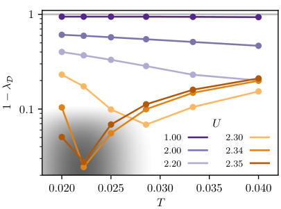
The same non-local Bethe-Salpeter kernel has appeared three times in stability criteria: in the Jacobian of the fixed point equation; in the compressibility; and in the second derivative of the self-energy functional. The latter two relate to the stability of the physical solution, whereas the Jacobian determines the attractiveness of the fixed point in an iterative scheme. For DMFT, these two aspects are tied together by a single kernel.
This allows us to create a unified picture of the hysteresis region of the particle-hole symmetric metal-insulator transition. At the critical end point , the purple dot in Fig. 1, the two stable (triangles in Fig. 1) and the one unstable (vertical marks in Fig. 1) stationary points merge together. Therefore, the quadratic part of the free energy functional vanishes at this point (purple curve), which together with Eq. (8) means that the Bethe-Salpeter kernel has an eigenvector with eigenvalue (Fig. 2) exactly at the critical end point. Since is related to the Jacobian of the fixed point equation, the stable and unstable solutions correspond to attractive and repulsive fixed points, respectively Strand et al. 2011.
Figure 3 shows the leading right eigenvector of close to the critical end point. The physical meaning of this eigenvector is that it relates the three fixed points that exist at , as and , where , and are the hybridization functions at the metallic, insulating and unstable fixed points, respectively, and is a critical exponent. This together with particle-hole symmetry [] implies , i.e., the eigenvector is antisymmetric Springer et al. 2020. As the difference between solutions, provides the “order parameter” – similar to Kotliar’s Kotliar 1999 at – in the sense of Landau’s functional: At the critical point, the free energy landscape goes from a parabola to a double well potential along the direction given by . Figure 4 shows that the second derivative of the grand potential – along the direction given by the right eigenvector of the Jacobian – indeed goes to zero as one gets close to the Mott critical end point. Note that the figure is at , so the second derivative does not quite reach zero.
Since at the critical point (cf. Fig. 3), the three solutions differ only at low frequency, i.e., close to the Fermi level. This is in agreement with what is known qualitatively from investigations of the Density of States: the difference between the insulator and the metal is that the latter has a quasiparticle peak at the Fermi level. Astretsov et al. Astretsov et al. 2020 used a single Matsubara frequency approximation to study the cuprates, our result here is a direct quantitative proof that this kind of approximation is justified at the critical end point of the Mott transition.
At and , the Bethe-Salpeter equation is convergent (and the iterative scheme is attractive) at both the metallic and the insulating solutions, , and divergent (repulsive) at the unstable fixed point, . Although both metallic and insulating solution are attractive fixed points, only one of them is the global minimum (c.f., green and orange curves in Fig. 1) of the free energy in most of the hysteresis region. Only at (the blue line in Fig. 1), both solutions have exactly the same free energy, this is where the phase transition occurs. At () the unstable and insulating (metallic) fixed point merge, so that at this fixed point, but the metallic (insulating) solution, with , is the global minimum of the free energy.
Kotliar et al. Kotliar et al. 2002 predicted a compressibility divergence at the critical end point of the doping-driven Mott transition, . On first sight, our present eigenvalue analysis seems to imply the same, since the BSE diverges. However, a divergence in the BSE can be canceled by an exact orthogonality Kotliar et al. 2002; Springer et al. 2020, and that is indeed what happens at particle-hole symmetry Reitner et al. 2020. The eigenvector is antisymmetric in and therefore does not contribute to the sum in Eq. (6) Chalupa et al. 2018; Springer et al. 2020; Reitner et al. 2020, so that , shown in Fig. 4, is finite (and small, Hafermann et al. 2014) at the critical end point. This is consistent with the absence of phase separation at particle-hole symmetry Eckstein et al. 2007. A non-divergent compressibility combined with a divergence of the BSE is reminiscent of the zero temperature case Krien et al. 2019, in other words, both critical end points of the particle-hole symmetric Mott transition are characterized by a divergent BSE without a divergence in .
The situation away from particle-hole symmetry is more complicated because of the complex-valuedness of the Green’s functions Reitner et al. 2020. The antiferromagnetic transition in DMFT Jarrell 1992 — which occurs when the assumption of paramagnetism is lifted — can also be analyzed along the lines of the current work as a divergence of the BSE in the magnetic channel. An important open question is the generalization of our analysis to the instabilities found in multi-orbital Hund’s physics Werner et al. 2008; Haule and Kotliar 2009; de’ Medici et al. 2009; de’ Medici et al. 2011; Werner et al. 2012; Stadler et al. 2015; de’ Medici 2017; Villar Arribi and de’ Medici 2018, and more generally to systems that show phase separation Grilli et al. 1991; Majumdar and Krishnamurthy 1994; Tandon et al. 1999; Held et al. 2001; Kotliar et al. 2002; Capone et al. 2004; Eckstein et al. 2007; Aichhorn et al. 2007; Lupi et al. 2010; Otsuki et al. 2014; Yee and Balents 2015.
In conclusion, we identified the non-local Bethe-Salpeter kernel with the Jacobian of the DMFT fixed point equation and with the curvature of the free energy functional. Near the critical end point of the finite temperature correlation-driven Mott transition the BSE diverges. The eigenvector corresponding to the divergence relates the insulating and metallic solutions that exist below the critical temperature. Particle-hole symmetry then implies that this eigenvector is antisymmetric and does not contribute to the compressibility Reitner et al. 2020, which remains finite.
Acknowledgements.
The authors thank M. Capone, P. Chalupa, H. Hafermann, M. Katsnelson, A. Lichtenstein, M. Schüler, A. Toschi, A. Valli and T. Wehling for stimulating discussions. E.G.C.P.v.L. is supported by the Zentrale Forschungsförderung of the Universität Bremen. F.K. acknowledges financial support from the Slovenian Research Agency under project number N1-0088. A.K. acknowledges partial financial support within the state assignment of Ministry of Science and Higher Education of the Russian Federation (theme “Quant” No. AAAA-A18-118020190095-4) and RFBR grant 20-02-00252.References
- Imada et al. (1998) M. Imada, A. Fujimori, and Y. Tokura, Rev. Mod. Phys. 70, 1039 (1998).
- Hubbard (1963) J. Hubbard, Proc. R. Soc. A. 276, 238 (1963).
- Kanamori (1963) J. Kanamori, Prog. Theor. Phys. 30, 275 (1963).
- Gutzwiller (1963) M. C. Gutzwiller, Phys. Rev. Lett. 10, 159 (1963).
- Hubbard (1964) J. Hubbard, Proc. R. Soc. A. 281, 401 (1964).
- Jördens et al. (2008) R. Jördens, N. Strohmaier, K. Günter, H. Moritz, and T. Esslinger, Nature 455, 204 (2008).
- Schneider et al. (2008) U. Schneider, L. Hackermüller, S. Will, T. Best, I. Bloch, T. A. Costi, R. W. Helmes, D. Rasch, and A. Rosch, Science 322, 1520 (2008).
- Jördens et al. (2010) R. Jördens, L. Tarruell, D. Greif, T. Uehlinger, N. Strohmaier, H. Moritz, T. Esslinger, L. De Leo, C. Kollath, A. Georges, V. Scarola, L. Pollet, E. Burovski, E. Kozik, and M. Troyer, Phys. Rev. Lett. 104, 180401 (2010).
- Duarte et al. (2015) P. M. Duarte, R. A. Hart, T.-L. Yang, X. Liu, T. Paiva, E. Khatami, R. T. Scalettar, N. Trivedi, and R. G. Hulet, Phys. Rev. Lett. 114, 070403 (2015).
- Greif et al. (2016) D. Greif, M. F. Parsons, A. Mazurenko, C. S. Chiu, S. Blatt, F. Huber, G. Ji, and M. Greiner, Science 351, 953 (2016).
- Metzner and Vollhardt (1989) W. Metzner and D. Vollhardt, Phys. Rev. Lett. 62, 324 (1989).
- Georges et al. (1996) A. Georges, G. Kotliar, W. Krauth, and M. J. Rozenberg, Rev. Mod. Phys. 68, 13 (1996).
- (13) New perspectives still appear, such as topological views on the transition Logan and Galpin 2015; Sen et al. 2020.
- Jarrell (1992) M. Jarrell, Phys. Rev. Lett. 69, 168 (1992).
- Georges and Krauth (1992) A. Georges and W. Krauth, Phys. Rev. Lett. 69, 1240 (1992).
- Georges and Krauth (1993) A. Georges and W. Krauth, Phys. Rev. B 48, 7167 (1993).
- Zhang et al. (1993) X. Y. Zhang, M. J. Rozenberg, and G. Kotliar, Phys. Rev. Lett. 70, 1666 (1993).
- Rozenberg et al. (1994) M. J. Rozenberg, G. Kotliar, and X. Y. Zhang, Phys. Rev. B 49, 10181 (1994).
- Noack and Gebhard (1999) R. M. Noack and F. Gebhard, Phys. Rev. Lett. 82, 1915 (1999).
- Bulla (1999) R. Bulla, Phys. Rev. Lett. 83, 136 (1999).
- Blümer (2002) N. Blümer, Mott-Hubbard Metal-Insulator Transition and Optical Conductivity in High Dimensions, Ph.D. thesis, University of Augsburg (2002).
- Eckstein et al. (2007) M. Eckstein, M. Kollar, M. Potthoff, and D. Vollhardt, Phys. Rev. B 75, 125103 (2007).
- Strand et al. (2011) H. U. R. Strand, A. Sabashvili, M. Granath, B. Hellsing, and S. Östlund, Phys. Rev. B 83, 205136 (2011).
- Schäfer et al. (2015) T. Schäfer, F. Geles, D. Rost, G. Rohringer, E. Arrigoni, K. Held, N. Blümer, M. Aichhorn, and A. Toschi, Phys. Rev. B 91, 125109 (2015).
- Khurana (1990) A. Khurana, Phys. Rev. Lett. 64, 1990 (1990).
- Zlatic and Horvatic (1990) V. Zlatic and B. Horvatic, Solid State Communications 75, 263 (1990).
- Pruschke et al. (1993) T. Pruschke, D. L. Cox, and M. Jarrell, Phys. Rev. B 47, 3553 (1993).
- Rozenberg et al. (1995) M. J. Rozenberg, G. Kotliar, H. Kajueter, G. A. Thomas, D. H. Rapkine, J. M. Honig, and P. Metcalf, Phys. Rev. Lett. 75, 105 (1995).
- Brener et al. (2008) S. Brener, H. Hafermann, A. N. Rubtsov, M. I. Katsnelson, and A. I. Lichtenstein, Phys. Rev. B 77, 195105 (2008).
- Rohringer et al. (2012) G. Rohringer, A. Valli, and A. Toschi, Phys. Rev. B 86, 125114 (2012).
- Boehnke and Lechermann (2012) L. Boehnke and F. Lechermann, Phys. Rev. B 85, 115128 (2012).
- van Loon et al. (2014) E. G. C. P. van Loon, H. Hafermann, A. I. Lichtenstein, A. N. Rubtsov, and M. I. Katsnelson, Phys. Rev. Lett. 113, 246407 (2014).
- Geffroy et al. (2019) D. Geffroy, J. Kaufmann, A. Hariki, P. Gunacker, A. Hausoel, and J. Kuneš, Phys. Rev. Lett. 122, 127601 (2019).
- Strand et al. (2019) H. U. R. Strand, M. Zingl, N. Wentzell, O. Parcollet, and A. Georges, Phys. Rev. B 100, 125120 (2019).
- Krien et al. (2019) F. Krien, E. G. C. P. van Loon, M. I. Katsnelson, A. I. Lichtenstein, and M. Capone, Phys. Rev. B 99, 245128 (2019).
- Melnick and Kotliar (2020) C. Melnick and G. Kotliar, Phys. Rev. B 101, 165105 (2020).
- Rubtsov et al. (2005) A. N. Rubtsov, V. V. Savkin, and A. I. Lichtenstein, Phys. Rev. B 72, 035122 (2005).
- Werner et al. (2006) P. Werner, A. Comanac, L. de’ Medici, M. Troyer, and A. J. Millis, Phys. Rev. Lett. 97, 076405 (2006).
- Gull et al. (2011) E. Gull, A. J. Millis, A. I. Lichtenstein, A. N. Rubtsov, M. Troyer, and P. Werner, Rev. Mod. Phys. 83, 349 (2011).
- Schäfer et al. (2013) T. Schäfer, G. Rohringer, O. Gunnarsson, S. Ciuchi, G. Sangiovanni, and A. Toschi, Phys. Rev. Lett. 110, 246405 (2013).
- Kozik et al. (2015) E. Kozik, M. Ferrero, and A. Georges, Phys. Rev. Lett. 114, 156402 (2015).
- Schäfer et al. (2016) T. Schäfer, S. Ciuchi, M. Wallerberger, P. Thunström, O. Gunnarsson, G. Sangiovanni, G. Rohringer, and A. Toschi, Phys. Rev. B 94, 235108 (2016).
- Gunnarsson et al. (2017) O. Gunnarsson, G. Rohringer, T. Schäfer, G. Sangiovanni, and A. Toschi, Phys. Rev. Lett. 119, 056402 (2017).
- Chalupa et al. (2020) P. Chalupa, T. Schäfer, M. Reitner, D. Springer, S. Andergassen, and A. Toschi, “Fingerprints of the local moment formation and its kondo screening in the generalized susceptibilities of many-electron problems,” (2020), arXiv:2003.07829 [cond-mat.str-el] .
- Stan et al. (2015) A. Stan, P. Romaniello, S. Rigamonti, L. Reining, and J. A. Berger, New Journal of Physics 17, 093045 (2015).
- Rossi and Werner (2015) R. Rossi and F. Werner, Journal of Physics A: Mathematical and Theoretical 48, 485202 (2015).
- Thunström et al. (2018) P. Thunström, O. Gunnarsson, S. Ciuchi, and G. Rohringer, Phys. Rev. B 98, 235107 (2018).
- Vučičević et al. (2018) J. Vučičević, N. Wentzell, M. Ferrero, and O. Parcollet, Phys. Rev. B 97, 125141 (2018).
- Tarantino et al. (2017) W. Tarantino, P. Romaniello, J. A. Berger, and L. Reining, Phys. Rev. B 96, 045124 (2017).
- Chalupa et al. (2018) P. Chalupa, P. Gunacker, T. Schäfer, K. Held, and A. Toschi, Phys. Rev. B 97, 245136 (2018).
- Springer et al. (2020) D. Springer, P. Chalupa, S. Ciuchi, G. Sangiovanni, and A. Toschi, Phys. Rev. B 101, 155148 (2020).
- Chitra and Kotliar (2001) R. Chitra and G. Kotliar, Phys. Rev. B 63, 115110 (2001).
- Potthoff (2003) M. Potthoff, The European Physical Journal B - Condensed Matter and Complex Systems 32, 429 (2003).
- Žitko (2009) R. Žitko, Phys. Rev. B 80, 125125 (2009).
- Reitner et al. (2020) M. Reitner, P. Chalupa, L. Del Re, D. Springer, S. Ciuchi, G. Sangiovanni, and A. Toschi, arXiv e-prints , arXiv:2002.12869 (2020), arXiv:2002.12869 [cond-mat.str-el] .
- Bauer et al. (2011) B. Bauer, L. D. Carr, H. G. Evertz, A. Feiguin, J. Freire, S. Fuchs, L. Gamper, J. Gukelberger, E. Gull, S. Guertler, A. Hehn, R. Igarashi, S. V. Isakov, D. Koop, P. N. Ma, P. Mates, H. Matsuo, O. Parcollet, G. Pawłowski, J. D. Picon, L. Pollet, E. Santos, V. W. Scarola, U. Schollwöck, C. Silva, B. Surer, S. Todo, S. Trebst, M. Troyer, M. L. Wall, P. Werner, and S. Wessel, Journal of Statistical Mechanics: Theory and Experiment 2011, P05001 (2011).
- Huang et al. (2015) L. Huang, Y. Wang, Z. Y. Meng, L. Du, P. Werner, and X. Dai, Comp. Phys. Comm. 195, 140 (2015).
- Huang (2017) L. Huang, Comp. Phys. Comm. 221, 423 (2017).
- Hafermann et al. (2013) H. Hafermann, P. Werner, and E. Gull, Computer Physics Communications 184, 1280 (2013).
- Hafermann et al. (2012) H. Hafermann, K. R. Patton, and P. Werner, Phys. Rev. B 85, 205106 (2012).
- (61) Here we ignore the possibility of mixing of previous and current iterative solutions, since we are interested in the fundamental aspects of the stability of DMFT solutions.
- Rubtsov et al. (2008) A. N. Rubtsov, M. I. Katsnelson, and A. I. Lichtenstein, Phys. Rev. B 77, 033101 (2008).
- Hafermann (2010) H. Hafermann, Numerical Approaches to Spatial Correlations in Strongly Interacting Fermion Systems, Ph.D. thesis, University of Hamburg (2010).
- Rohringer et al. (2018) G. Rohringer, H. Hafermann, A. Toschi, A. A. Katanin, A. E. Antipov, M. I. Katsnelson, A. I. Lichtenstein, A. N. Rubtsov, and K. Held, Rev. Mod. Phys. 90, 025003 (2018).
- van Loon et al. (2015) E. G. C. P. van Loon, H. Hafermann, A. I. Lichtenstein, and M. I. Katsnelson, Phys. Rev. B 92, 085106 (2015).
- Kotliar (1999) G. Kotliar, The European Physical Journal B - Condensed Matter and Complex Systems 11, 27 (1999).
- Kotliar et al. (2000) G. Kotliar, E. Lange, and M. J. Rozenberg, Phys. Rev. Lett. 84, 5180 (2000).
- Astretsov et al. (2020) G. V. Astretsov, G. Rohringer, and A. N. Rubtsov, Phys. Rev. B 101, 075109 (2020).
- Kotliar et al. (2002) G. Kotliar, S. Murthy, and M. J. Rozenberg, Phys. Rev. Lett. 89, 046401 (2002).
- Hafermann et al. (2014) H. Hafermann, E. G. C. P. van Loon, M. I. Katsnelson, A. I. Lichtenstein, and O. Parcollet, Phys. Rev. B 90, 235105 (2014).
- Werner et al. (2008) P. Werner, E. Gull, M. Troyer, and A. J. Millis, Phys. Rev. Lett. 101, 166405 (2008).
- Haule and Kotliar (2009) K. Haule and G. Kotliar, New Journal of Physics 11, 025021 (2009).
- de’ Medici et al. (2009) L. de’ Medici, S. R. Hassan, M. Capone, and X. Dai, Phys. Rev. Lett. 102, 126401 (2009).
- de’ Medici et al. (2011) L. de’ Medici, J. Mravlje, and A. Georges, Phys. Rev. Lett. 107, 256401 (2011).
- Werner et al. (2012) P. Werner, M. Casula, T. Miyake, F. Aryasetiawan, A. J. Millis, and S. Biermann, Nature Physics 8, 331 (2012).
- Stadler et al. (2015) K. M. Stadler, Z. P. Yin, J. von Delft, G. Kotliar, and A. Weichselbaum, Phys. Rev. Lett. 115, 136401 (2015).
- de’ Medici (2017) L. de’ Medici, Phys. Rev. Lett. 118, 167003 (2017).
- Villar Arribi and de’ Medici (2018) P. Villar Arribi and L. de’ Medici, Phys. Rev. Lett. 121, 197001 (2018).
- Grilli et al. (1991) M. Grilli, R. Raimondi, C. Castellani, C. Di Castro, and G. Kotliar, Phys. Rev. Lett. 67, 259 (1991).
- Majumdar and Krishnamurthy (1994) P. Majumdar and H. R. Krishnamurthy, Phys. Rev. Lett. 73, 1525 (1994).
- Tandon et al. (1999) A. Tandon, Z. Wang, and G. Kotliar, Phys. Rev. Lett. 83, 2046 (1999).
- Held et al. (2001) K. Held, A. K. McMahan, and R. T. Scalettar, Phys. Rev. Lett. 87, 276404 (2001).
- Capone et al. (2004) M. Capone, G. Sangiovanni, C. Castellani, C. Di Castro, and M. Grilli, Phys. Rev. Lett. 92, 106401 (2004).
- Aichhorn et al. (2007) M. Aichhorn, E. Arrigoni, M. Potthoff, and W. Hanke, Phys. Rev. B 76, 224509 (2007).
- Lupi et al. (2010) S. Lupi, L. Baldassarre, B. Mansart, A. Perucchi, A. Barinov, P. Dudin, E. Papalazarou, F. Rodolakis, J.-P. Rueff, J.-P. Itié, et al., Nature communications 1, 105 (2010).
- Otsuki et al. (2014) J. Otsuki, H. Hafermann, and A. I. Lichtenstein, Phys. Rev. B 90, 235132 (2014).
- Yee and Balents (2015) C.-H. Yee and L. Balents, Phys. Rev. X 5, 021007 (2015).
- Logan and Galpin (2015) D. E. Logan and M. R. Galpin, Journal of Physics: Condensed Matter 28, 025601 (2015).
- Sen et al. (2020) S. Sen, P. J. Wong, and A. K. Mitchell, “The Mott transition as a topological phase transition,” (2020), arXiv:2001.10526 [cond-mat.str-el] .
I Supplemental material: Conventions and detailed derivations
I.1 The auxiliary impurity model: thermodynamic potential and its derivatives
The auxiliary impurity model is a central object in DMFT. In the action formalism, it is defined as
where are Grassmann numbers, are their Fourier transform, and . The corresponding thermodynamic potential reads
| (9) |
Accordingly, the first derivative of the thermodynamic potential with respect to the hybridization yields the single-particle Green’s function of the impurity,
| (10) |
and the second derivative yields
| (11) |
We relate the two-particle Green’s function to the local vertex by
| (12) |
which yields
| (13) |
where is the local charge susceptibility. Comparing this to
| (14) |
we finally obtain the useful relation
| (15) |
I.2 The Jacobian of DMFT self-consistency
We analyze the stability of DMFT iterations in terms of , the usual input of impurity solvers. In the DMFT self-consistency condition , appears explicitly on the right-hand side, since , but it also appears implicitly on both sides through the (non-invertible Kozik et al. 2015) functional relation . In an iterative scheme we obtain as
| (16) |
where is considered as a functional of . Taking the derivative of Eq. (16) we obtain
| (17) |
where is the local Green’s function. From this we obtain
| (18) |
Using the derivative of the self-energy (15) we obtain
| (19) |
where the non-local Bethe-Salpeter kernel is defined by the Equation (4) of the main text. The eigenvalues of the Jacobian (19) remain smaller than one for the physical solutions, which is provided by the eigenvalues of smaller than one.
I.3 Bethe-Salpeter equation and the non-local kernel
The Bethe-Salpeter equation is a relation between the full vertex and the so-called irreducible vertex . For the full local vertex in the charge channel (here, as well as in the main text we consider zero bosonic frequency ) we have the Bethe-Salpeter equation
| (20) |
where , as in the main text. The solution of Eq. (20) is
| (21) |
We have previously seen that is the derivative of the self-energy with respect to , Eq. (15). As somewhat similar relation can be derived for the irreducible vertex . However, in that case the derivative is done with respect to the full impurity Green’s function, whereas the derivative in Eq. (15) is with respect to a bare object. The relation is not always invertible Kozik et al. 2015 and this leads to divergences in already on the level of an impurity model, whereas is divergence free (at ). By defining physical observables in terms of instead of , we can avoid complications arising from these local divergences.
The generalized susceptibility in DMFT is given by
| (22) |
Note that we have defined and generalized susceptibility so that both are positive, after being summed over Matsubara frequencies, and our sign convention for is opposite to Georges et al. Georges et al. 1996, who use .
Our goal is to get rid of in favor of in this expression. The Bethe-Salpeter Equation (20) allows us to write
| (23) |
leading to the result
| (24) |
Equation (22) is a geometric series consisting of repeated particle-hole scattering: is the scattering and is the propagation of the particle-hole pair. The latter has both a local and a non-local component, successive scattering events can occur at the same or at different sites. Equation (24) is a resummation of this result, where all successive scatterings on the same site are collected in . The propagatoin between scatterings is then necessarily non-local and given by . Finally, the term in the prefactor ensures that processes where the first propagation is local are also included.
For the non-local vertex we find similarly to the Eq. (21)
| (25) |
This equation can be rewritten as
| (26) |
where and the kernel is defined by Eq. (4). We note that while the eigenvalues of are positive in the stable phases, the eigenvalues of , and, consequently, do not have in general a definite sign, and therefore can not be used to study stability of various phases.
I.4 Second derivative of the Landau functional
The first derivative of the functional is given by the Eq. (7) of the main text. For the second derivative of this functional we obtain
| (27) |
Differentiating the self-consistency condition , where is given by the Eq. (2), we find
| (28) |
Therefore,
| (29) |
Combining this with the Eq. (13), we find at the stationary point ()
| (30) |
Although is generally a complex function, at particle-hole symmetry is purely imaginary (modulo the constant Hartree contribution), so it is sufficient to look at . We show in the next subsection of Supplementary Material that the denominator in Eq. (30) is positive in the region of interest and we write
| (31) |
At the critical point, one eigenvalue of the Hessian changes sign, the corresponding eigenvector determines the unstable direction of the free energy landscape.
Here, the leading eigenvector of the Jacobian provides the relevant direction. It is convenient to start from the right eigenvector of with eigenvalue ,
| (32) |
and the associated conjugated vector with normalization
| (33) |
The right eigenvector of the Jacobian is related to the right eigenvector of the non-local Bethe-Salpeter kernel, with the same eigenvalue , in accordance with Eq. (19). This leads to and is consistent with the normalization ( and can be seen as co- and contravariant vectors in a space with metric ). For the combination shown in Fig. 4 we obtain
| (34) |
which goes to zero at the critical end-point, since .
I.5 Relation between different functionals
Here we consider the reformulation of the functional originally suggested in Ref. Chitra and Kotliar 2001, which is appropriate to establish the relation to our functional. To this end we perform Legendre transform
| (35) |
such that
| (36) |
Furthermore, we invert the map and denote its inverse by . We note that while the functional can be multivalued (see next subsection), its inverse is well defined. Finally, we introduce the functional , such that . Such a functional necessarily exists since is frequency-diagonal, and can be therefore simply integrated over . Therefore, we obtain
| (37) |
Differentiating once more over and using the relations (13) and (29), we find
| (38) |
The obtained derivative (38) is analogous to the derivative of the Baym-Kadanoff functional , discussed in Ref. Chitra and Kotliar 2001. Using the hybridization in Eq. (37) yields straightforwardly the DMFT self-consistency equation, without the need of passing to another functional, in the notation of Ref. Chitra and Kotliar 2001.
However, the vertex may diverge at some interaction strengths in the strong coupling regime, which makes the eigenvalues of the Eq. (38), as well as the second derivative of the functional of Ref. Chitra and Kotliar 2001 not positive definite. The same concerns the functional of Ref. Potthoff 2003. To emphasize further the relation of Eq. (38) to our result of Eq. (8) of the main text, we transform Eq. (38) as
| (39) |
We see that the considered derivative is related to the derivative of in the following way
| (40) |
Despite the non-explicitly symmetric form of this equation, it is symmetric under , which can be once more verified by rewriting
such that
This shows the symmetry and returns us back to the Eq. (38).
Let us discuss conditions of sign definiteness of the considered second derivatives. The second derivative of is proportional to appearing from the derivative . This makes the derivative not sign definite near MIT, which is related to multivaluedness of the map . The multiplier is absent in the derivative of the functional , considered in this paper. However, this comes at the price of the new factor in Eq. (30), which may not be positive definite. As one can see from the derivation in the previous section, this factor can be traced back to the derivative . This derivative is not always positive definite, which is in turn related to possible multivaluedness of the map (see next section). The advantage of using is however that at strong coupling one can consider only one relevant branch of the functional as discussed in the following section. This makes the factor positive definite in the strong coupling regime. In general, this reflects dichotomy of describing the system in terms of at weak coupling vs. at strong coupling.
I.6 Sign of the non-local bubble
The sign of the non-local bubble can be ascertained by analyzing the (lattice) Green’s function in terms of and . Particle-hole symmetry implies that the real numbers are distributed symmetrically around zero and that is purely imaginary (after cancellation of the Hartree part with the chemical potential). To compress the notation, we introduce () and write
| (41) |
Let us rewrite the non-local bubble in terms of the density of states :
| (42) |
In the limit of large the Eq. (42) is proportional to the second moment of the density of states, and, therefore, positive. At small using the low energy behavior of the density of states of the square lattice, ( is the half bandwidth) and keeping singular contributions, we obtain
| (43) |
Numerical analysis shows that change of the sign of the dual bubble occurs at . This corresponds to local Green function . The change of the sign of the bubble is entirely related to the van Hove singularity of the density of states, which yields the first term in the right hand side of Eq. (43), proportional to the derivative of the density of states , much bigger than the second term, proportional to . For smooth densities of states both and remain finite for and the sign of the bubble is given by the competition of these terms. For the Bethe lattice and the simple cubic lattice we find that the bubble remains positive for all .
According to the relation (29), vanishing of the non-local bubble corresponds to the divergence of the derivative . This occurs since the function (we can discuss it here as a function instead of a functional, since it is diagonal in frequency) is two-valued, see Fig. 5. The corresponding values of join each other at , where ). The functional , inverse to , is also diagonal in frequency and well defined.
In the regime of small and the corresponding values of are small at low frequencies, and the DMFT solution belongs to the ”upper” branch of the function for these frequencies, while it belongs to the lower branch for higher frequencies. The increase of and/or shifts, however, the DMFT solution to the lower branch of the function for all Matsubara frequencies, making the corresponding functional well-defined. This also stresses universality of the Mott transition, since only one branch of the functional is present for the prototypical example of Mott transition – the Hubbard model on the Bethe lattice – reflecting above discussed absence of a sign change of the non-local bubble for this lattice.