Microscopic theory for nematic fractional quantum Hall effect

For condensed matter systems with non-trivial topological orders, the robustness of the topological properties at low temperature usually requires the ground state to have a finite energy gap to all excitations in the thermodynamic limitprange. In general for such systems, the universal topological features dominate the ground state response, and the geometric properties of the system are less important. The incompressible FQH states are such examples where topological orders arise from strong interactions between electrons, without needing protection of any symmetry. There are also examples of compressible FQH states with no plateau formation for the Hall conductivity, with anisotropic stripe or bubble phases that are gapless and spontaneously break the rotational/translational symmetrywest1; west2; west3; west4; klitzing; lin; csathy; smet; manfra. An interesting exception is the nematic fractional quantum Hall effect (FQHN), which was recently discovered in experimentsxia; west5. Here we have examples where topological orders and non-trivial geometric effects coexist: there is an anisotropic longitudinal resistivity enhanced by low temperature, and at the same time with a robust plateau for Hall conductivity.

It is generally believed that the robustness of the Hall conductivity plateau in FQHN is due to the finite charge gap, while the anisotropic longitudinal resistivity is a result of the neutral excitations in the long wavelength limit becoming gaplessjoseph. Such neutral excitations form a degenerate ground state manifold. They are thus prone to spontaneous symmetry breaking. It is well known that the neutral excitations in the long wavelength limit is a quadrupole excitation that breaks rotational symmetry, potentially leading to anisotropic transportyangbo1; regnault. Non-trivial geometric effects also arise in experiments where rotational symmetry is explicitly brokenmansour1; mansour2. Several field theoretical studies of the FQHN have been carried out, either by assuming that the neutral excitations go soft in the long wavelength limitjoseph, or by adding an attractive quadrupolar interactionyizhi; rezayi. These theories capture the topological order, the nematic order from spontaneous symmetry breaking, as well as the neutral and charge gapsgromov1; gromov2; gromov3 in a phenomenological manner.

Microscopic theories are needed to better understand the assumptions used in the field theoretical approaches. For the FQHN most studies so far are based on numerical computations. Finite system analysis has established that the single mode approximation (SMA) is exact for the neutral excitations in the long wavelength limityangbo1. This is true from numerical calculations for all accessible system sizes, and is expected to be true in the thermodynamic limit. The Jack polynomial formalism, the composite fermion picture and the first quantised form of the neutral excitations are also constructed to shed more insights on the nature of such many-body statesyangbo1; sreejith; ajit1; ajit2; yangbo2; gromov. Numerical studies have tentatively shown that short range interactions can lead to instability of the intrinsic guiding center metric, and such “squeezed” Laughlin states can harbour uniform nematic orderregnault. It is, however, difficult to show microscopically how assumptions in the FQHN field theory can arise from bare interactions between electrons with numerical studies. In particular, important physics happening at long wavelength limit is inaccessible given the relatively small system sizes that can be computed numerically.

In this paper, we compute analytically the conditions for the long wavelength limit (small $q$) of the neutral excitation to go soft in the thermodynamic limit. Using the Laguerre polynomials as the basis, variational energies of the neutral excitations at small $q$ is controlled by two universal, tridiagonal characteristic matrix $\Gamma_{\left(1\right)},\Gamma_{\left(2\right)}$ that can be computed exactly and are independent of microscopic details. The SMA at small $q$ becomes exact eigenstates when it is degenerate with the ground state, and we can identify it with the guiding center metric deformation of the ground state. Thus the onset of the FQHN can be understood as the case when the shear modulus of the gapped ground state of the quantum fluid vanisheshaldane3.

We also identify trial wavefunctions for the gapless nematic mode from spontaneous symmetry breaking, where the spatially varying “nematic wave” can be shown explicitly. While $\Gamma_{\left(1\right)}$ controls the neutral excitation gap, the dispersion of the nematic mode is controlled by $\Gamma_{\left(2\right)}$. The tridiagonal nature of $\Gamma_{\left(1\right)}$ and $\Gamma_{\left(2\right)}$ implies the dynamics of the FQHN only depends on the long wavelength part of the ground state structure factor, if the interaction is short-ranged. The analysis here can much simplify the numerical computation of the nematic phase and its finite size scaling. The derived results are applicable to FQH phases at any filling factor. The necessary analytic conditions for the robustness of the FQHN phases are also illustrated with numerical calculations using the Laughlin state at filling factor $\nu=1/3$ as an example.

The FQHN phase at $\nu=n+1/3$ is also special, because we can show that the quadrupole excitations are exact zero modes of the Haffnian model Hamiltonian. We will thus use it as an example to illustrate the validity of the general methodologies (both analytic and numerical) proposed in this paper. The connection to the Haffnian state also allows us to derive a family of two-body interactions supporting robust FQHN in the presence of strong magnetic field, which can be realised experimentally with suitable tuning of the sample thickness and interaction screening. We also show the presence of Landau level (LL) mixing can potentially help stabilise FQHN in higher LLs, pointing to diverse conditions for the experimental observations of the FQHN in the neighbourhood of the fully gapped Laughlin phase.

This paper will be organised as follows: In Sec. II we compute the long wavelength energy gap of the neutral excitations from the SMA in the thermodynamic limit, and show that it is determined by the universal characteristic matrix $\Gamma_{\left(1\right)}$. We term such neutral excitations in the long wavelength limit as the quadrupole excitations. In Sec. III we show the quadrupole excitations can be identified as a uniform area-preserving deformation of the ground state, both from the wavefunction and the energetics perspectives. Thus the quadrupole excitations harbour uniform nematic orderregnault. In Sec. IV we derive the expression of the spatially varying nematic order from the trial wavefunctions of the gapless nematic mode in the FQHN phase. We also show the quadratic dispersion of the nematic mode is controlled by another universal characteristic matrix $\Gamma_{\left(2\right)}$. In Sec. V we analytically investigate several families of short range microscopic models, and derive conditions for the FQHN to be viable. In Sec. VI we carry out preliminary numerical analysis focusing on the Laughlin phase at filling factor $\nu=1/3$, corroborating with the analytical results to show tentative evidence of FQHN when the two-body interaction is a family of linear combinations of the $\hat{V}_{1}^{\text{2bdy}},\hat{V}_{3}^{\text{2bdy}}$ and $\hat{V}_{5}^{\text{2bdy}}$ pseudopotentials derived from eigenstates of $\Gamma_{\left(1\right)}$. In Sec. VII we discuss about the contrasting natures of the quadrupole and dipole neutral excitations at $\nu=n+1/3$, showing the interesting connection of the quadrupole excitations to the Haffnian model Hamiltonian, with various experimental implications. In Sec. VIII we summarize the results of this paper and discuss about the future works.

Let us start with a two-body Hamiltonian in a single Landau level (LL) as follows:

where $\hat{\rho}_{\bm{q}}=\sum_{i}e^{iq_{a}\hat{R}_{i}^{a}}$ is the guiding center density operator, and $\hat{R}^{a}_{i}$ are the guiding center coordinates with only matrix elements between states in the same Landau level. It also satisfies the commutation relation $[\hat{R}_{i}^{a},\hat{R}_{i}^{b}]=-i\epsilon^{ab}l_{B}^{2}$, where $l_{B}$ is the magnetic length. The number of electrons is given by $N_{e}$ and we set $l_{B}=1$. Assuming at a fixed filling factor, Eq.(1) is incompressible with both neutral and charged quasielectron gaps, with ground state $|\psi_{0}\rangle$ and energy $E_{0}$. Defining the regularised guiding center density as $\delta\hat{\rho}_{\bm{q}}=\hat{\rho}_{\bm{q}}-\langle\psi_{0}|\hat{\rho}_{\bm{q}}|\psi_{0}\rangle=\hat{\rho}_{\bm{q}}-\frac{N_{e}\delta\left(q\right)}{2\pi q}$ with $q=|\bm{q}|$, the GMP algebragmp is given by:

The regularised ground state structure factor is defined as $S_{\bm{q}}=\langle\psi_{0}|\delta\hat{\rho}_{\bm{q}}\delta\hat{\rho}_{-\bm{q}}|\psi_{0}\rangle$ and we also have the following relationship for fermionshaldane1; haldane2:

We now start with the family of SMA trial wavefunctions $|\psi_{\bm{q}}\rangle=\delta\hat{\rho}_{\bm{q}}|\psi_{0}\rangle$, which are orthogonal to the ground state with variational energies $E_{\bm{q}}$. The variational energy gap is thus given bysup:

Here we assume rotational invariance. In the long wavelength limit, the ground state structure factor is given by $\lim_{|q|\rightarrow 0}S_{\bm{q}}=\eta q^{4}$, where $\eta=N_{e}\kappa/2$ and $\kappa$ is bounded below by the Hall viscosity of the ground statehaldane3. By expanding Eq.(5) to the leading order in $q$, and using Eq.(3), we have the following expression:

Here $q_{1}=|q^{\prime}|^{2},q_{2}=|q^{\prime\prime}|^{2}$, and $\prescript{}{0}{\mathbf{F}}_{1}\left(a,x\right)$ is the regularised hypergeometric functionsup. For very short range interactions (e.g. with $\hat{V}_{1}^{\text{2bdy}}$ pseudopotentialprange), $\delta E_{\bm{q}\rightarrow 0}>0$ and is buried in the continuum of multi-roton excitations. If $V_{\bm{q}}$ in Eq.(1) can be tuned such that $\delta E_{\bm{q}\rightarrow 0}\rightarrow 0$, then $|\psi_{\bm{q}}\rangle$ becomes an exact eigenstate, degenerate with $|\psi_{0}\rangle$, given that there is no level crossing from $\hat{V}_{1}^{\text{2bdy}}\rightarrow V_{\bm{q}}$.

To evaluate the numerator in Eq.(II), we first note that due to the property of the structure factor in Eq.(3), $s_{\bm{q}}$ is a linear combination of Laguerre polynomials $L_{m}\left(q^{2}\right)$ with odd $m$. Expanding $V_{\bm{q}}$ in the same basis of Laguerre polynomials, we have the following:

Note the two-body Haldane pseudopotential interaction Hamiltonians are also given by the Laguerre polynomials:

Using the Hardy–Hille formula, Eq.(9) can be further simplified to give:

where both $m,n$ are odd integers, and $\Gamma^{mn}_{\left(1\right)}$ is a tridiagonal matrix. It is then useful to treat $V_{\bm{q}},s_{\bm{q}}$ as vectors $\bm{c},\bm{d}$ respectively, in the basis of Laguerre polynomials, where $\bm{d}$ is completely from the ground state. The dot product $\bm{c}\cdot\bm{d}$ gives the ground state energy $E_{0}$, and the variational energy gap is given by the inner product:

Note that $\Gamma_{\left(1\right)}$ is a well-defined mathematical function given by Eq.(11), while the only physical input to the Hamiltonian is given by $\bm{c}$. There is a one-to-one mapping of $\bm{d}$ from $\bm{c}$, with the ground state of Eq.(1). For short range interactions with $c_{m}=0$ for $m>m_{0}$, we only need to consider $d_{n}$ with $n\leq m_{0}+2$. A more detailed analysis will be presented in Sec. V.

We now explore the nematic order of the neutral excitations in the long wavelength limit by connecting them to the anisotropic ground state from deforming the guiding center metric of $|\psi_{0}\rangle$. The area-preserving deformation generators can be defined as $\hat{\Lambda}^{ab}=\frac{1}{4}\sum_{i}\{\hat{R}_{i}^{a},\hat{R}_{i}^{b}\}$ with the following closed algebrahaldane3:

The family of anisotropic ground states can thus be defined as $|\xi_{\theta,\phi}\rangle=e^{i\alpha_{ab}\hat{\Lambda}^{ab}}|\psi_{0}\rangle$, with $\alpha_{ab}$ as a symmetric matrix. The Bogoliubov transformation of the guiding center coordinates is given by $\hat{R}^{\prime a}=\lambda_{b}^{a}\hat{R}^{b}=e^{-i\alpha_{cd}\hat{\Lambda}^{cd}}\hat{R}^{a}e^{i\alpha_{cd}\hat{\Lambda}^{cd}}$, thus $|\xi_{\theta,\phi}\rangle$ is the ground state of Eq.(1) with the transformation in $V_{\bm{q}}$: $q_{a}\rightarrow\left(\lambda^{-1}\right)_{a}^{b}q_{b}$, or $q^{2}\rightarrow g^{ab}q_{a}q_{b}$, where $g^{ab}$ is a unimodular metric parametrised as follows:

For the rotationally invariant $|\psi_{0}\rangle$, the variational energy of $|\xi_{\theta,\phi}\rangle$ only depends on $\theta$, which parameterises the squeezing of the metric, as followssup:

Comparing Eq.(12) and Eq.(17), we can see the variational energy of the neutral excitations in the long wavelength limit is related to the shear modulous $\langle\bm{c},\bm{d}\rangle_{\Gamma_{\left(1\right)}}$ of the ground state. Thus for small $|\bm{q}|$ and $\theta$, $|\psi_{\bm{q}}\rangle$ and $|\xi_{\theta,\phi}\rangle$ approximately have the same energy with $\theta=1/\left(2\sqrt{\eta}\right)$.

In general $|\psi_{\bm{q}\rightarrow 0}\rangle$ and $|\xi_{\theta\rightarrow 0,\phi}\rangle$ do not have to be related to each other even when they have the same variational energy. However when $\langle\bm{c},\bm{d}\rangle_{\Gamma_{\left(1\right)}}\rightarrow 0$, they will belong to the same manifold of degenerate ground states. Denoting $\phi_{\bm{q}}$ as the angle of the momentum, we can identify the following at small $q$ based on inversion symmetry, as long as $|\psi_{\bm{q}}\rangle$ are the only states degenerate with the ground state:

This is the ground state of the FQHN after spontaneous symmetry breaking, and finite size numerical analysis indicates that $|\xi_{\theta,\phi}\rangle$ could have uniform nematic orderregnault. Thus in the long wavelength limit, $|\psi_{\bm{q}}^{\pm}\rangle$ is equivalent to the guiding center metric deformation of the ground state at $\bm{q}=0$, if the shear modulus $\langle\bm{c},\bm{d}\rangle_{\Gamma_{\left(1\right)}}$ vanishes. This leads to the development of the nematic order for the neutral excitations in this limit.

The long wavelength spatial modulation of the nematic order should gives rise to the gapless excitations that are related to the Goldstone mode. To identify these states let us first define the operator of the local nematic order, which is a slightly modified version fromregnault:

where $\bm{l}$ is an arbitrary point-splitting vector, $\theta_{\bm{l}}$ is the angle of $\bm{l}$, and $\delta\hat{\rho}\left(\bm{r}\right)$ is the Fourier component of $\delta\hat{\rho}_{\bm{q}}$. For a translationally invariant state $|\psi_{0}\rangle$, the nematic order is independent of $\bm{r}$, and we have:

where $s_{\tilde{\bm{l}}}$ is defined by Eq.(3) with $\tilde{l}_{a}=l_{B}^{-2}\epsilon_{ab}l^{b}$, $l_{B}$ being the magnetic length. Eq.(20) is clearly zero if $|\psi_{0}\rangle$ is rotationally invariant, and non-zero if the structure factor has a quadrupole symmetry. For the nematic ground state established in Eq.(18), simple algebra gives us:

where $\mathcal{N}_{q}^{\left(1\right)},\mathcal{N}_{q}^{\left(2\right)}$ are two non-universal functions of $q$ that can be computed analyticallysup. Thus at least when $q$ is small enough, $|\psi^{\pm}_{\bm{q}}\rangle$ is the nematic mode with spatially varying nematic order given by the second term in Eq.(21).

To look at the dispersion of this nematic wave, we can expand Eq.(5) to the next order. When Eq.(12) vanishes at the FQHN phase, we havesup:

It is important to note that the dispersion of the gapless nematic mode is quadratic. The necessary condition for the FQHN phase is thus $\langle\bm{c},\bm{d}\rangle_{\Gamma_{\left(1\right)}}=0,\langle\bm{c},\bm{d}\rangle_{\Gamma_{\left(2\right)}}>0$. Both $\Gamma_{\left(1\right)}$ and $\Gamma_{\left(2\right)}$ are universal tridiagonal matrices independent of the microscopic details of the Hamiltonians.

Effective field theories generally predicts a linear gapless Goldstone mode in the FQHN phase, from the long wavelength fluctuation of the nematic directorjoseph; yizhi; gromov1. The velocity of this Goldstone mode vanishes at the quantum critical point (QCP) when the neutral mode becomes degenerate with the ground state, leading to a quadratic dispersion from the nematic amplitude fluctuation. The microscopic theory agrees with this effective description in the neighbourhood of the QCP with $\langle\bm{c},\bm{d}\rangle_{\Gamma_{\left(1\right)}}\sim 0$, where the analytical derivation of the variational energies and the quantum states are exact. Deep in the isotropic phase where $\langle\bm{c},\bm{d}\rangle_{\Gamma_{\left(1\right)}}>0$, our calculations will only be accurate if the SMA still gives good variational wavefunctions of these Hamiltonians.

It is important to highlight that deep in the nematic phase when $\langle\bm{c},\bm{d}\rangle_{\Gamma_{\left(1\right)}}<0$ and the global ground state is no longer isotropic, the long wavelength SMA may not be good trial wavefunctions. This could lead to the microscopic theory here not able to capture the linear Goldstone mode, and it does not preclude the existence of such linear dispersions away from the critical point. On the other hand, moving deep into the nematic phase generally implies moving further away from the model Hamiltonians of the fully gapped FQH states, which will likely close the charge gap and destroy the FQHN phase. Gapless smectic or stripe phases are expected especially in higher LLs. It is also worth noting that unlike quantum Hall ferromagnets, the nematic director in FQHN are not really physically measurable quantities. Both the fluctuations of the nematic amplitude and the nematic director lead to the fluctuation of the nematic order defined in Eq.(19), associated with the quadratic gapless dispersion. Further investigations are warranted both for the effective and the microscopic theories in the nematic phase far away from the QCP.

To understand the dynamics of the FQHN phase from microscopic Hamiltonians analytically as much as possible, we start with spectrum of $\Gamma_{\left(1\right)}$, which is real given that the matrix is symmetric. The eigenvalues $\lambda_{1}$ and corresponding eigenvectors $\vec{c}^{\lambda_{1}}$ satisfy the following relationship:

where $k$ is a non-negative odd integer and $c^{\lambda_{1}}_{-1}=0$. In particular, if the microscopic two-body interaction is $\vec{c}=\vec{c}^{\lambda_{1}}$, we then have $\lim_{\bm{q}\rightarrow 0}\delta E_{\bm{q}}=\left(\lambda_{1}E_{0}\right)/\left(256\eta\right)$, where $E_{0}=\vec{c}\cdot\vec{d}$ is the ground state energy in the $\bm{q}=0$ sector. It is easy to check that $\lambda_{1}=0$ gives $c^{0}_{k}=\textit{const}$, which is not relevant for realistic interactions.

We now focus on a special family of interactions with $\vec{c}$ such that $c_{k}=c^{\lambda_{1}}_{k}$ for $k\leq k_{0}$, and $c_{k}=0$ for $k>k_{0}$. These are interactions from the eigenvectors of $\Gamma_{\left(1\right)}$ but with a cut-off. For the more realistic case where $c_{k}$ decreases with $k$, we need to have $\lambda_{1}<0$. Simple algebra leads to:

Thus the variational energy gap requires three inputs from numerical computations: $d_{k_{0}},d_{k_{0}+2}$ and the ground state energy $E_{0}$. This relationship is valid at any filling factor in the thermodynamic limit.

All results in Sec. V are valid in the thermodynamic limit, and are applicable at any filling factor. In this section, we perform some preliminary numerical analysis at filling factor $\nu=1/3$, about possible microscopic models for the FQHN. While we are looking at a particular filling factor, the methodologies for the numerical analysis described here can be applied to any filling factors. A more specialised analysis of the FQHN states for the Laughlin phase will be given in the next section.

We will show that the analytic derivations from the previous sections can strongly constrain the parameter space for the realisation of FQHN in the thermodynamic limit. Thus numerically, we only need to look for the FQHN phase over a much smaller parameter space in the form of the linear combination of pseudopotentials. All numerical computations in this work are done with the spherical geometryhaldane4, and we analyse the ground state wavefunctions and energy spectra for reasonably large system sizes. While the comparison between finite size scaling of numerical results and the analytical results in Sec. V can never be conclusive, the results here nevertheless illustrate the usefulness and limitations of finite size numerical calculations.

The neutral gap of $\delta E_{\bf q\rightarrow 0}$ in this section is not computed from the energy spectrum. Instead we use Eq.(12) to evaluate the energy gap numerically from the ground state in the $L=0$ sector alone. Not only is this a simpler calculation technically, it also has smaller finite size effect. This is because $\Gamma_{\left(1\right)}$ is calculated from the thermodynamic limit and the only size dependent quantity is $\bm{d}$. In addition, it allows us to compute the energy gap in the limit $\bf q\rightarrow 0$, which is inaccessible from the full spectra of the finite systems.

For the model Hamiltonian consisting of only $\hat{V}_{1}^{\text{2bdy}}$ pseudopotential (i.e. $c_{1}=1,c_{i>1}=0$, or the $k_{0}=1$ model), there are no tuning parameters, and the variational energy gap of the SMA state is completely controlled by $d_{3}-d_{1}$ (see Eq.(27)). In Fig.(2), we scan over all possible combinations of $N_{e},N_{o}$ that are numerically accessible, and compute $d_{1},d_{3}$ from the ground state in the $L=0$ sector (not necessarily the global ground state). The numerical results show strong evidence that for any FQH phases that can potentially be supported by the $k_{0}=1$ model (which in particular includes many Abelian Jain states), the SMA states in the long wavelength limit is gapped from the ground state in the $L=0$ sector.

An interesting observation is that with the $\hat{V}_{1}^{\text{2bdy}}$ model Hamiltonian and for all finite size systems we have accessed, the global ground state is in the $L=0$ sector if and only if the filling factor and the topological shift corresponds to the Jain series, i.e. $N_{o}=\left(2n+1\right)N_{e}/n-n-1$, and their particle-hole conjugates. These Hilbert spaces are highlighted in Fig.(2). For all of these cases we have $d_{1}/d_{3}<1$, indicating gapped neutral excitations as $|q|\rightarrow 0$. For other combinations of $N_{e},N_{o}$ where the global ground state is not in the $L=0$ sector, it could be because the neutral excitations go soft even for finite size systems (probably of unknown filling factors), and they could still have a charge gap. However in all cases where $N_{o}$ is reasonably large, $d_{1}/d_{3}<1$ as well. There is thus no numerical evidence of the FQHN. For each $N_{e}$, $d_{1}/d_{3}>1$ only when $N_{o}$ is rather small. This implies as $N_{e}$ increases, we can only have $d_{1}/d_{3}>1$ at rather large filling factors ($\nu\gtrsim 0.75$).

We now move onto $k_{0}=3$ model Hamiltonians that are linear combinations of $\hat{V}_{1}^{\text{2bdy}}$ and $\hat{V}_{3}^{\text{2bdy}}$ pseudopotentials, where without loss of generality we set $c_{1}=1$. From the general expression of Eq.(V.2), the allowed range of $c_{3}$ and $d_{5}/d_{3}$ is given in the shaded area in Fig.(3a), which is computed analytically in the thermodynamic limit. In particular, the FQHN phase is not possible in the thermodynamic limit for $0.123<c_{3}<0.462$. Any numerical evidence suggesting otherwise is due to finite size effects.

For the Laughlin phase at $\nu=1/3$, finite size analysis is carried out at different values of $c_{3}$, at which $d_{5}/d_{3}$ is computed from the ground state (in the $L=0$ sector). They show that it is very unlikely for $d_{5}/d_{3}$ to be below the maximally allowed value (see Fig.(3a) inset) at all possible values of $c_{3}$. The scaling shows that the variational energy gap (first line of Eq.(V.2)) also seems to be finite, which is consistent (see Fig.(3b)). While the finite size energy spectrum does seem to indicate softening of the neutral mode in the long wavelength limit (see Fig.(3b) inset) for some values of $\lambda_{1}$, that most likely will not be the case when larger system sizes become accessible numerically.

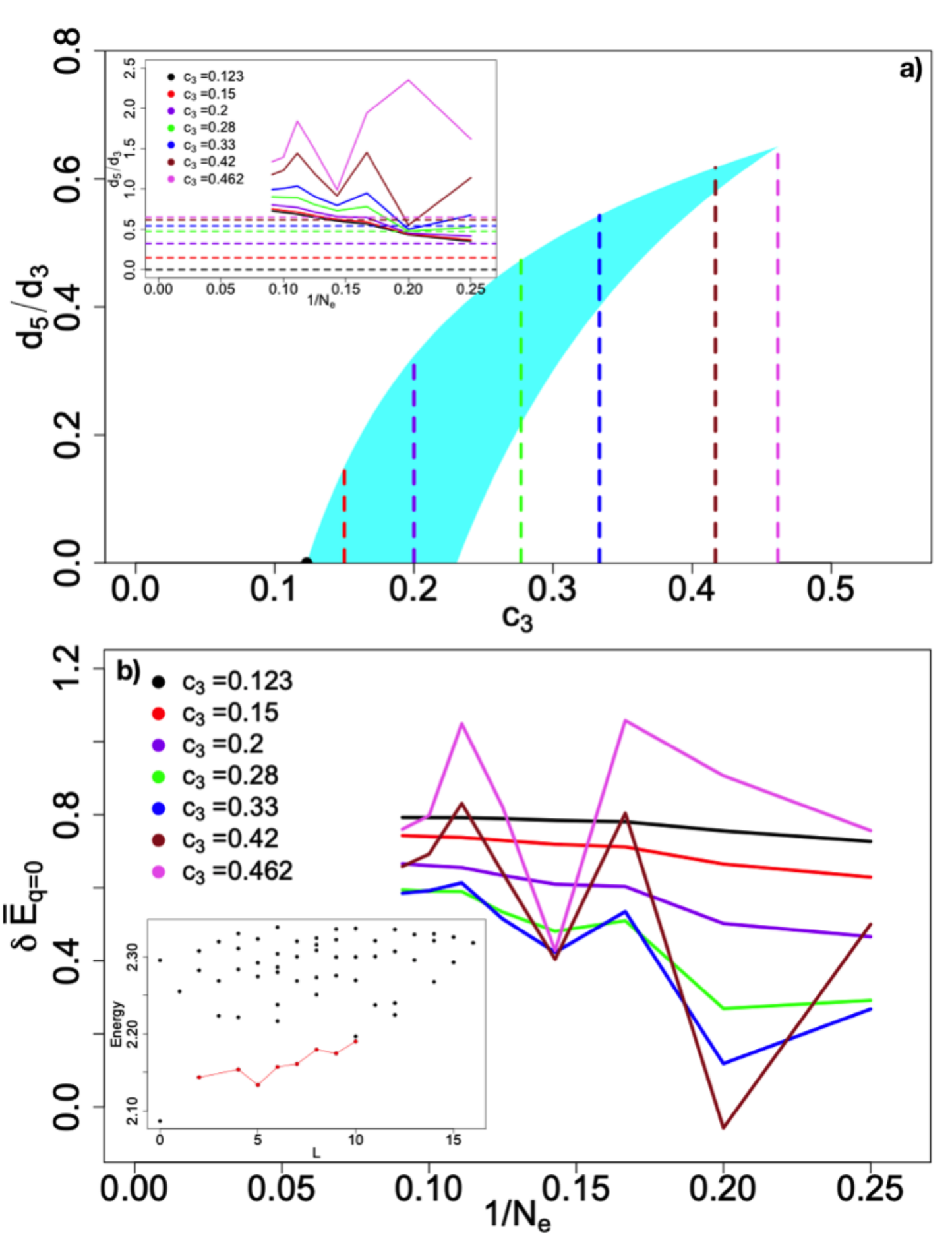
For $k_{0}=5$ model Hamiltonians, the addition of $\hat{V}_{5}^{\text{2bdy}}$ introduces additional variables $c_{5}$ and $d_{7}$, making thorough numerical investigation difficult. We look at the special case when $\vec{c}$ comes from the eigenvectors of $\Gamma_{\left(1\right)}$, i.e. $c_{i}=c_{i}^{\lambda_{1}}$ for $i=1,3,5$, and $c_{i>5}=0$. From the analytic expression of Eq.(V.3), we have rigorous results on the range of $c_{3}$ in different scenarios. At filling factor $\nu=1/3$ numerical computations show it is unlikely for $d_{3}/d_{5}>2$ in the thermodynamic limit for a wide range of $c_{1}>c_{3}>c_{5}$. For each value of $d_{3}/d_{5}$, we can analytically calculate the possible range of $c_{3},d_{7}/d_{5}$ from Eq.(V.3) for the FQHN phase. The results are plotted in Fig.(1). In particular, only a small range of $c_{3}$ needs to be explored for the potential realisation of the FQHN at $\nu=1/3$.

Since there is a unique relationship between $\lambda_{1}$ and $\left(c_{3},c_{5}\right)$, different values of $\lambda_{1}$ are plotted in Fig.(4), by diagonalising the full Hilbert space and extracting $d_{i}$ from the corresponding ground states. In the limit of $N_{e}\rightarrow\infty$, $d_{3}/d_{5}$ seems to fall in between $0.5$ and $1.5$ (see Fig.(4a)). From Fig.(1) we thus need $d_{7}\sim 0.7$ (without being too precise), and this also seems quite possible from Fig.(4b). For $\lambda_{1}<-3.5$, the finite size scaling of Eq.(V.3) seems to clearly indicate that $\delta E_{\bm{q}\rightarrow 0}$ does not go soft. On the other hand, for $\lambda_{1}>-3.2$, the finite size effect becomes strong, potentially indicating the divergence of the ground state correlation length and the closing of the neutral gap in the long wavelength limit (see Fig.(4c)).

We thus expect the minimal microscopic model for the FQHN at $\nu=1/3$ consists of a linear combination of $\hat{V}_{1}^{\text{2bdy}},\hat{V}_{3}^{\text{2bdy}},\hat{V}_{5}^{\text{2bdy}}$. The results here apply to zero temperature, where spontaneous symmetry breaking can only happen at $\delta E_{\bm{q}\rightarrow 0}=0$. It is possible to have a range of parameters for the FQHN phase to be stable, especially if the interaction is allowed to be more long ranged. At finite temperature, FQHN phase can be observed as long as the neutral excitation gap $\delta E_{\bm{q}\rightarrow 0}$ is much smaller than the charge gap $\Delta E_{c}$, and the former is smaller than the thermal energy $k_{B}T$, i.e. $\delta E_{\bm{q}\rightarrow 0}\ll k_{B}T\ll\Delta E_{c}$. Thus in realistic experimental setting, the FQHN phase could be stable against disorder and small perturbations, as long as the charge gap is the dominant energy scale.

While the previous sections describe analytic and numerical methodologies for studying generic FQHN phases at any filling factors, in this section we reveal more special properties of the Laughlin phase at $\nu=1/3$ that are relevant to the FQHN. Not only does these special properties allow us to extend the general results derived in the previous sections, it also leads to much better understandings of the nature of the softening of the neutral modes at $\nu=1/3$. A number of favourable experimental conditions are also proposed, which can lead to more robust realisation of the FQHN phase and even the observation of Haffnian-like FQH stateshf1; hf2, as we will explain below.

We have computed analytically the dynamical behaviours of the neutral excitations in the long wavelength and thermodynamic limit, which is applicable to any FQH phase with a charge gap. Such excitations are quadrupole excitations, with its gap and dispersion relations captured by two universal tridiagonal matrices that are independent of microscopic details. Both the nematic order and the gapless modes from spatially varying nematic order are studied, and we can show that such nematic wave dispersion is quadratic at the quantum critical point. Specific criteria for the FQHN phase to be robust are also derived, which are necessary (though not sufficient) conditions for the coexistence of the anisotropic transport and the topologically protected Hall conductivity plateau.

In addition, we show that the gap of the quadrupole excitation and its dispersion in long wavelength limit can be completely determined from the ground state properties, given the universality of the characteristic matrices in the thermodynamic limit. This provides a new approach in studying the potential transition from isotropic to FQHN phases both analytically and numerically at the microscopic level. Numerical analysis on the Laughlin phase at filling factor $\nu=1/3$ for reasonably large system sizes shows evidence that the phase transition is only likely for microscopic Hamiltonians that are linear combinations of at least three leading Haldane pseudopotentials (i.e. $\hat{V}_{1}^{\text{2bdy}},\hat{V}_{3}^{\text{2bdy}},\hat{V}_{5}^{\text{2bdy}}$). We also show at this filling factor the FQHN is strongly connected to the Haffnian phase, a competing topological phase at the same filling factor but with a different topological shift. The analytical results can narrow down the parameter range for the short range interactions, allowing us to see tentative evidence of the softening of the neutral excitations in the fermionic systems. Several favourable experimental conditions are proposed where the neutral gap in the long wavelength limit is likely to be much smaller than the charge gap.

The characteristic matrices derived in this work shows that the dynamics of the quadrupole excitations has universal aspects that can potentially be useful for constructing effective theories for the FQH effects. From the microscopic perspective, more work is needed to fully understand the competition between the quadrupole gap and dipole gap for different FQH phases. The latter essentially gives the charge gap of the FQH fluid, and needs to be finite for the quantum fluid to be incompressible. Our results tentatively suggests that while short range interaction generally support a finite charge or dipole gap, it can nevertheless lead to softening of the quadrupole gap. For example the $k_{0}=5$ model Hamiltonians we analysed in the paper has a much shorter range than the lowest Landau level Coulomb interaction. On the other hand, for very short range interaction (e.g. $k_{0}=1$ or $k_{0}=3$ models), the quadrupole gap becomes very large and merge into the multi-roton continuum. The underlying physics of such behaviours is still not well understood.

In our numerical analysis we ignored the $q^{4}$ coefficient of the structure factor, which is the denominator of the quadrupole gap. This should be justified since it is bounded from below by the Hall viscosityhaldane3. Perturbation from the $V_{1}$ model Hamiltonian should only have the possibility of increasing the coefficient (thus reducing the quadrupole gap further). Nevertheless, more detailed numerical analysis is needed to see if including the $q^{4}$ coefficient can give clearer finite scaling of various aspects of the quadrupole excitations. The results in this work is also applicable for any filling factors. It is interesting to explore the possibility of the FQHN phases in other filling factors, especially for the non-Abelian phases where there are multiple branches of the low-lying neutral modes.

Starting with SMA trial wavefunction $|\psi_{\bm{q}}\rangle=\delta\hat{\rho}_{\bm{q}}|\psi_{0}\rangle$, where $\delta\hat{\rho}$ is defined in the main text and $|\psi_{0}\rangle$ is the ground state of the two-body effective Hamiltonian $\mathcal{H}$ in the $\bm{q}=0$ sector (where $\bm{q}$ is the linear momentum), we compute the following commutation:

Using the GMP algebra, the second term vanishes, we thus have:

References

- (1) Bo Yang, Z.-X. Hu, Z. Papic and F.D.M. Haldane, Phys. Rev. Lett. 108, 256807 (2012).