An ALMA Survey of H2CO in Protoplanetary Disks
Abstract
H2CO is one of the most abundant organic molecules in protoplanetary disks and can serve as a precursor to more complex organic chemistry. We present an ALMA survey of H2CO towards 15 disks covering a range of stellar spectral types, stellar ages, and dust continuum morphologies. H2CO is detected towards 13 disks and tentatively detected towards a 14th. We find both centrally-peaked and centrally-depressed emission morphologies, and half of the disks show ring-like structures at or beyond expected CO snowline locations. Together these morphologies suggest that H2CO in disks is commonly produced through both gas-phase and CO-ice-regulated grain-surface chemistry. We extract disk-averaged and azimuthally-averaged H2CO excitation temperatures and column densities for four disks with multiple H2CO line detections. The temperatures are between 20-50K, with the exception of colder temperatures in the DM Tau disk. These temperatures suggest that H2CO emission in disks is generally emerging from the warm molecular layer, with some contributions from the colder midplane. Applying the same H2CO excitation temperatures to all disks in the survey, we find that H2CO column densities span almost three orders of magnitude (). The column densities appear uncorrelated with disk size and stellar age, but Herbig Ae disks may have less H2CO compared to T Tauri disks, possibly because of less CO freeze-out. More H2CO observations towards Herbig Ae disks are needed to confirm this tentative trend, and to better constrain under which disk conditions H2CO and other oxygen-bearing organics efficiently form during planet formation.
Subject headings
astrochemistry, protoplanetary disks, ISM: molecules, radio lines: ISMI. Introduction
Protoplanetary disks are the precursors of planetary systems. These disks consist of gas and dust orbiting young stars. Over time, the dust grains collide and stick together to form pebbles, eventually growing into planetesimals and planets (e.g. Mordasini et al. 2008, and references therein). The organic compositions of pebbles, planetesimals, and planets are therefore shaped by the organic chemistry of the gas and dust in their ancestral disks. By studying this chemistry, we can ultimately model and predict the chemical formation environment of young planets (Cridland et al. 2016; Öberg & Bergin 2016; Cridland et al. 2017, e.g.) and their potential ability to develop Earth-like life.
The small organic molecule formaldehyde (H2CO) is expected to be important for the overall organic chemical budget of disks. H2CO is commonly and abundantly detected in disks (Dutrey et al. 1997; Aikawa et al. 2003; Thi et al. 2004; Öberg et al. 2010; Öberg et al. 2011, e.g.,). Based on cometary observations, H2CO was also abundant in the solar nebula; in comets it is present at levels of 0.1-1% with respect to water (Mumma & Charnley 2011). There are several possible chemical origins of H2CO in disks. H2CO can form through neutral-neutral gas-phase chemistry (Fockenberg & Preses 2002; Atkinson et al. 2006, e.g.,), and through grain-surface chemistry via CO ice hydrogenation (Hiraoka et al. 1994; Hiraoka et al. 2002; Watanabe & Kouchi 2002; Hidaka et al. 2004; Watanabe et al. 2004; Fuchs et al. 2009, e.g.,). Both processes can occur in disks, though likely in different locations, since neutral-neutral gas-phase chemical reactions increase with density and temperature towards the inner disk, while CO ice hydrogenation is only possible beyond the CO snowline. In addition, H2CO has been detected in ices around young stellar objects (Gibb et al. 2004; Pontoppidan et al. 2004; Boogert et al. 2008, e.g., detections/tentative detections by), and some of the H2CO observed in disks might be inherited from this preceding evolutionary stage (Drozdovskaya et al. 2014; Drozdovskaya et al. 2019, e.g.,).
Understanding H2CO emission and its origins in disks is important for modeling more complex organic disk chemistry. When formed through CO-ice hydrogenation, H2CO serves as a stepping-stone towards forming oxygen-bearing, complex organic molecules (Herbst & van Dishoeck 2009, known as COMs, and typically defined as unsaturated carbon-bearing molecules with five or more atoms; e.g.,), especially methanol (Hiraoka et al. 1994; Watanabe & Kouchi 2002, CH3OH; e.g.,). COMs are expected to be rich in disks based on astrochemical disk models (Walsh et al. 2014). Unfortunately, without the help of rare heating phenomena such as stellar outbursts (van ’t Hoff et al. 2018; Lee et al. 2019, e.g.,), COM emission lines are predicted to be difficult to detect in disks (Henning & Semenov 2013; Walsh et al. 2014), due to their large partition functions and comparatively small abundances. To date, the largest COMs detected towards disks are cyanoacetylene (Chapillon et al. 2012, HC3N,), methyl-cyanide (Öberg et al. 2015b, CH3CN,), methanol (Walsh et al. 2016, CH3OH,), and formic acid (Favre et al. 2018, HCOOH,), and only cyanoacetylene and methyl-cyanide have been detected in more than one disk (Bergner et al. 2018; Loomis et al. 2018). H2CO, on the other hand, is readily detectable in disks. The presence/absence of H2CO emission, originating specifically from grain-surface chemistry, can thus indicate whether the disk hosts a rich organic grain-surface chemistry or not (Walsh et al. 2014; Öberg et al. 2017).
The chemical origins of H2CO in disks, and its potential to form more complex organic chemistry, can be addressed through spatially-resolved observations of H2CO emission at millimeter and submillimeter wavelengths. To date, H2CO has been spatially resolved with the Atacama Large Millimeter/submillimeter Array (ALMA) towards six disks: (1) the T Tauri disk Oph IRS 48 (van der Marel et al. 2014); (2) the T Tauri disk DM Tau (Loomis et al. 2015); (3) the Herbig Ae disk HD 163296 (Carney et al. 2017; Guzmán et al. 2018); (4) the T Tauri disk TW Hya (Öberg et al. 2017); (5) the T Tauri disk V4046 Sgr (Kastner et al. 2018); and (6) the T Tauri disk DG Tau (Podio et al. 2019). These six studies show a variety of H2CO morphologies, from centrally peaked (indicative of gas-phase formation) to ring-like in the outer disk (indicative of formation through CO ice hydrogenation). Two of these studies (Carney et al. 2017; Guzmán et al. 2018) calculated H2CO excitation temperatures of 20K and 24K, which are consistent with both formation pathways. Three of these studies (Loomis et al. 2015; Carney et al. 2017; Öberg et al. 2017) determined that the detected H2CO emission could be described by two distinct components of H2CO: (1) a warm inner component produced through gas-phase chemistry, and (2) a cold outer component exterior to the CO snowline produced through grain-surface chemistry. A larger survey of H2CO emission towards disks is necessary to explore the typical distribution and chemical origins of H2CO in protoplanetary disks, as well as their connections to stellar and disk characteristics.
In this work, we present an ALMA survey of H2CO towards 15 protoplanetary disks. We characterize the H2CO morphologies, excitation temperatures, and column densities, evaluate their dependence on stellar and disk characteristics, and assess the chemical origins of H2CO. In Section II, we describe the disk sample, the ALMA observations, and the data reduction process. In Section III, we present our methodology for visualizing and analyzing the imaged line emission. In Section IV, we report the detections of H2CO, the H2CO emission morphologies, excitation temperatures, and column densities, and any trends relating the H2CO to stellar and disk characteristics. In Section V, we discuss the results in the context of H2CO formation chemistry and disk environment, and in Section VI we summarize the key findings from our survey.
II. Observational Details
II.1. Disk Sample
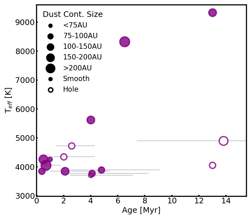
Figure 1 and Table 1 summarize the stellar and disk characteristics of the 15 disks in our sample. The sample was assembled from three main ALMA observing projects, with H2CO lines from other ALMA observing projects added in as available. The sample consists of well-studied T Tauri and Herbig Ae disks, and gas, dust, and temperature structures are available for most sources from previous studies. The host stars in the sample range in luminosity, mass, and age from 0.2-26L☉, 0.5-2.0M☉, and 1-15Myrs, respectively. All disks in the sample are relatively close by, 70-170pc away. Six disks in the sample are associated with the Taurus-Auriga region, five with the Upper Scorpius region, and one each with the Lupus and Ophiuchus regions.
The disks vary in dust morphology and size, but most are large. Outer millimeter dust radii range from 75 AU to 200 AU (where we define the outer radius as the radius where the azimuthally-averaged continuum emission drops below 5% of the peak). Five of the disks are “transition disks”, i.e. have large inner holes in their submillimeter/millimeter dust continuum: DM Tau (Marsh & Mahoney 1992), GM Aur (Jensen & Mathieu 1997), J1604-2130 (Mathews et al. 2012), LkCa 15 (Bergin et al. 2004), and V4046 Sgr (Jensen & Mathieu 1997).
| Disk | Stellar | R.A.[0] | Dec.[0] | Dist | Age∗ | L∗ | M∗ | Teff |
|---|---|---|---|---|---|---|---|---|
| Type | [J2000] | [J2000] | [pc] | [Myr] | [L☉] | [M☉] | [K] | |
| AS 209[1] | K5 | 16:49:15.3 | -14:22:09.0 | 121 | 1.0 | 1.41 | 0.83 | 4266 |
| CI Tau[2] | K7 | 04:33:52.0 | +22:50:29.8 | 159 | 0.7 (0.4-1.8) | 1.20 | 0.66 | 4060 |
| DM Tau[2] | M1 | 04:33:48.7 | +18:10:9.7 | 145 | 4.0 (2.5-7.1) | 0.24 | 0.53 | 3705 |
| DO Tau[2] | M0 | 04:38:28.6 | +26:10:49.1 | 140 | 0.4 (0.1-0.9) | 1.40 | 0.45 | 3850 |
| GM Aur[2] | K5.5[3] | 04:55:11.0 | +30:21:59.0 | 159 | 2.6 (1.4-4.3) | 1.60 | 1.30 | 4730 |
| HD 143006[1] | G7 | 15:58:36.9 | -22:57:15.5 | 165 | 4.0 | 3.80 | 1.78 | 5623 |
| HD 163296[1] | A1 | 17:56:21.3 | -21:57:22.5 | 101 | 13 | 17 | 2.04 | 9333 |
| IM Lup[1] | K5 | 15:56:09.2 | -37:56:06.5 | 158 | 0.5 | 2.57 | 0.89 | 4266 |
| J16042165-2130284∗[2] | K2 | 16:04:21.6 | -21:30:28.9 | 149 | 13.8 (7.4-32) | 0.62 | 1.11 | 4900 |
| J16090075-1908526∗[2] | K9 | 16:09:00.7 | -19:08:53.1 | 137 | 4.8 (2.5-9.1) | 0.32 | 0.68 | 3890 |
| J16123916-1859284∗[2] | M0.5 | 16:12:39.2 | -18:59:28.9 | 138 | 4.1 (1.8-8.3) | 0.29 | 0.56 | 3775 |
| J16142029-1906481∗[2] | M0 | 16:14:20.3 | -19:06:48.5 | 143 | 2.1 (1.0-5.4) | 0.46 | 0.60 | 3850 |
| LkCa 15[2] | K5 | 04:39:17.8 | +22:21:03.1 | 158 | 2.0 (0.9-4.3) | 1.04 | 1.03 | 4350 |
| MWC 480[2] | A4.52 | 04:58:46.3 | +29:50:36.6 | 161 | 6.5 | 25 | 1.84 | 8330 |
| V4046 Sgr∗∗[4] | K5,K7[5] | 18:14:10.5 | -32:47:35.3 | 73 | 13 | 0.86 | 1.75 | 4350, 4060 |
Note. — R.A. and Dec. (Columns 3 and 4) are from GAIA (Gaia Collaboration et al. 2016a; Gaia Collaboration et al. 2016b; Gaia Collaboration et al. 2018, e.g.,). All other table values are taken from the literature. For AS 209, HD 143006, HD 163296, and IM Lup, we use values as updated by [2] using new GAIA distances. For disks denoted by [1], we use values calculated/scaled using the same methodology of [2] unless otherwise individually referenced. For V4046 Sgr, we take all values except for the stellar type from [4], which assumed a distance of 73pc. Stellar ages (Column 6) are given as ranges in parentheses (which account for error) when available. : The disks J16042165-2130284, J16090075-1908526, J16123916-1859284, and J16142029-1906481 are referred to respectively as J1604-2130, J1609-1908, J1612-1859, and J1614-1906 in subsequent figures, tables, and text. : V4046 Sgr is a protoplanetary disk orbiting a binary star system. The individual stellar effective temperatures and total stellar luminosity and mass are reported. [0] Gaia Collaboration et al. 2016a; Gaia Collaboration et al. 2016b; Gaia Collaboration et al. 2018, [1] Andrews et al. 2018, [2] Calculated using the same methodology as Andrews et al. 2018, [3] Espaillat et al. 2010, [4] Rosenfeld et al. 2012, [5] Quast et al. 2000.
| H2CO | Freq. | Aul | Eu | gu | ALMA | Observed |
|---|---|---|---|---|---|---|
| Line | [GHz] | [s-1] | [K] | Project Code | Disks | |
| p-303-202 | 218.222 | 2.818 | 20.956 | 7 | 2016.1.00627.S | CI Tau, DM Tau, DO Tau |
| 2015.1.00964.S | HD 143006, J1604-2130, J1609-1908, J1612-1859, J1614-1906 | |||||
| p-322-221 | 218.476 | 1.571 | 68.094 | 7 | 2015.1.00964.S | HD 143006, J1604-2130, J1609-1908, J1612-1859, J1614-1906 |
| 2013.1.00226.S | AS 209, HD 163296, IM Lup, LkCa 15, MWC 480, V4046 Sgr | |||||
| p-321-220 | 218.760 | 1.578 | 68.111 | 7 | 2015.1.00964.S | HD 143006, J1604-2130, J1609-1908, J1612-1859, J1614-1906 |
| 2013.1.00226.S | AS 209, HD 163296, IM Lup, LkCa 15, MWC 480, V4046 Sgr | |||||
| o-414-313 | 281.527 | 5.884 | 45.570 | 27 | 2015.1.00657.S | LkCa 15, MWC 480 |
| p-404-303 | 290.623 | 6.903 | 34.904 | 9 | 2015.1.00678.S | AS 209, DM Tau, GM Aur, IM Lup, V4046 Sgr |
| 2012.1.00681.S | HD 163296 | |||||
| 2015.1.00657.S | LkCa 15, MWC 480 | |||||
| p-423-322 | 291.238 | 5.211 | 82.071 | 9 | 2015.1.00657.S | LkCa 15, MWC 480 |
| p-422-321 | 291.948 | 5.249 | 82.122 | 9 | 2015.1.00657.S | LkCa 15, MWC 480 |
| o-413-312 | 300.837 | 7.178 | 47.887 | 27 | 2015.1.00657.S | LkCa 15, MWC 480 |
| o-515-414 | 351.769 | 12.02 | 62.452 | 33 | 2011.0.00629.S | DM Tau, MWC 480 |
Note. — ‘o-’ and ‘p-’ denote ortho and para lines, respectively. All frequencies, Einstein coefficients (Aul), upper energy levels (Eu), and degeneracies (gu) were obtained from the Cologne Database for Molecular Spectroscopy (Endres et al. 2016, CDMS;).
II.2. ALMA Observations
The core of our study contains observations of the H2CO 303-202 and 404-303 lines towards eight disks each (both lines are observed towards one disk, DM Tau). These observations are complemented by the H2CO 515-414 line towards two disks; the H2CO 322-221 and 321-220 lines towards 11 disks each; and the H2CO 414-313, 413-312, 423-322, and 422-321 lines towards two disks each. When detected, these additional lines are used to determine H2CO excitation temperatures and column densities.
In total, nine H2CO lines were considered, providing a total of 48 H2CO observations across the 15 disks. All H2CO lines and their molecular characteristics, ALMA observing projects, and corresponding disks are listed in Table 2. The ALMA observing projects are described and referenced briefly in Table 3.
We also consider complementary dust continuum and C18O observations towards all disks except GM Aur. All CO observations were taken from ALMA observing projects 2013.1.00226.S, 2015.1.00964.S, and 2016.1.00627.S.
| 2016.1.00627.S, 6 | 22-26 | 47 | 15-704 | 4-5 | Bergner et al. 2019 |
| 2015.1.00964.S, 6 | 14-21 | 48 | 15-704 | 5-10 | Bergner et al. 2019 |
| 2015.1.00678.S, 7 | 20 | 41 | 20-640 | 2.6-4.2∗ | Kastner et al. 2018; Qi et al. 2019 |
| 2015.1.00657.S, 7 | 23-61 | 39-44 | 15-650 | 5 | Loomis et al. (subm.) |
| 2013.1.00226.S, 6 | 12-21 | 31-37 | 20-784 | 6 | Huang et al. 2017 |
| 2012.1.00681.S, 7 | 45 | 32 | 18-650 | 2.9∗ | Qi et al. 2015 |
| 2011.0.00629.S, 7 | 35 | 23 | 17.5-380 | 6 | Loomis et al. 2015 |
Note. — ∗: The H2CO 404-303 line towards DM Tau, HD 163296, and V4046 Sgr was observed with largest angular scales of 2”.6, 2”.9, and 4”.2, respectively. It is possible that we are missing extended H2CO emission for these large disks.
II.3. Data Reduction
The ALMA/NAASC staff performed the initial calibration (including bandpass, flux, and phase calibration) for each observation. The flux calibration for HD 163296 in ALMA observing projects 2012.1.00681.S and 2013.1.00226.S was further optimized by Qi et al. 2015 and Huang et al. 2017, respectively. As the datasets were observed at different times across the past decade, we note that this initial calibration was non-uniform across the sample. After initial calibration, we used the Common Astronomy Software Applications package (CASA) version 4.7.2 to self-calibrate and image each targeted line. We self-calibrated using the continuum emission from all available spectral windows, after removing any strong lines. Solution intervals were 10-100 seconds. We used intervals within this range that maximized the number of solutions with signal-to-noise ratios 2. We carried out 2 iterations of phase calibration and 1 iteration of amplitude calibration for each line, and we used a Briggs weighting scheme and a robust value of 0.5 during the self-calibration process for all disks. There were a few exceptions to this approach. For one observation of the H2CO 413-312 line towards MWC 480, we used 3 iterations of phase calibration and 2 iterations of amplitude calibration to improve phase and amplitude solutions. We did not self-calibrate the H2CO 404-303 line towards DM Tau, or the H2CO 303-202 line towards J1612-1859, due to low continuum peaks for these sources.
After self-calibration, we subtracted out the continuum using CASA’s uvcontsub function and imaged each targeted line using CASA’s clean algorithm. We initially used a Briggs weighting scheme and a robust value of 0.5 for cleaning for all disks. We created the cleaning masks by hand to cover the emission and little else in each channel. For the weaker lines (e.g., H2CO 322-221), we recycled clean masks from the stronger lines available. The weaker H2CO lines that were tentatively-detected or non-detected with robust=0.5 were reimaged with robust=2 to maximize sensitivity.
We did not image the two weaker H2CO 322-221 and 321-220 lines for the disks J1609-1908, J1612-1859, and J1614-1906, because the emission from the much brighter H2CO 303-202 line was already very faint for these three disks.
III. Image Analysis

Our basic image products were image cubes, which are visualized as channel maps. Figure 2 displays the channel map for the H2CO 303-202 line towards J1604-2130; channel maps for all detected lines and sources are shown in Figure Sets A1-A3 in the Appendix. We generated Keplerian masks (Rosenfeld et al. 2013; Yen et al. 2016; Salinas et al. 2017, e.g.,) to extract the line emission within each channel for each disk, ultimately reducing the noise incorporated into the extracted emission. We generated each set of Keplerian masks in four steps11 1 The Keplerian mask package is available on GitHub (https://github.com/jpegues/kepmask). Version 1.0.0 was used for this paper and is available at https://doi.org/10.5281/zenodo.3382082.: (1) calculate each disk’s line-of-sight velocities within the disk’s coordinate system, (2) incorporate thermal and turbulent broadening using the approach of Yen et al. 2016, (3) mask the pixels within each velocity channel that fall within the broadened velocity bins, and (4) convolve the masks with the average beam size. For this survey, we empirically fit for the position and inclination angles using the masks, C18O emission towards each disk, and a grid-search algorithm (12CO emission was used for the three disks where C18O was not detected, and H2CO emission was used for the one disk where no CO was observed). The Keplerian masks calculated for the H2CO 303-202 line towards J1604-2130 are overplotted in the channel map of Figure 2. All parameters used to generate the Keplerian masks for the sample are given in Table 1 in the Appendix.
We created a velocity-integrated emission map (a.k.a. a moment-0 map) for each line and disk pair by summing up the emission within the Keplerian masks across the velocity channels in the data cube. To estimate the noise of each velocity-integrated emission map, it is important to account for how each pixel in the image appears in a different number of Keplerian masks, depending on the pixel’s location. We therefore generated an ‘rms map’ for each line and disk, which calculates the rms at each pixel through all masks. Each rms map has the same dimensions as the velocity-integrated emission map and holds different rms values for each pixel. For each line and disk, we randomly sampled 1000 rms maps across channels with no emission, and then took the standard deviation at each pixel. We used the median of the standard deviations as the estimate of the line emission map’s noise (). See Bergner et al. 2018 for the full methodology for generating rms maps.
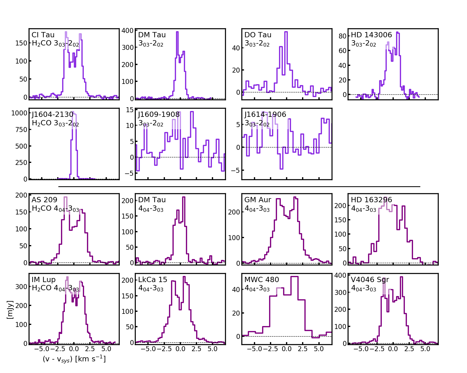
Velocity-integrated fluxes for each line and disk were calculated by summing over the velocity-integrated emission maps pixel-by-pixel. Noise was estimated similarly to the velocity-integrated maps, i.e. from the standard deviation of 1000 random samples. To create a radial emission profile for each line, we azimuthally averaged each velocity-integrated emission map. In this process, we deprojected the disks and divided them into 0.1” rings about the host star, and then averaged the emission within each ring. Following Bergner et al. 2018, we estimated the noise within each ring as (), where is the number of independent measurements in this ring, taken to be the number of pixels in the ring divided by the beam area (in pixels). For rings within the beam’s circumference, we fixed to be the beam circumference (in pixels) divided by the beam area. Finally, we summed the emission in the Keplerian masks as a function of velocity channel to extract a spectrum for each line and disk (shown in Figure 1 in the Appendix).
IV. Results
IV.1. Detection Statistics
| Disk | H2CO | Flux∗ | Peak Flux∗ | Int. Vel. | Chan. | rms∗∗ | Beam | Robust | |
|---|---|---|---|---|---|---|---|---|---|
| Line | [mJy | [mJy beam-1 | Range | Width | [mJy | Size (P.A.) | Value | ||
| km s-1] | km s-1] | [km s-1] | [km s-1] | beam-1] | |||||
| AS 209 | 404-303 | 580 17 | 19 2.6 | 0.9 - 8.1 | 0.4 | 2.9 | 0.31” x 0.22” (-69.84∘) | 0.5 | |
| 322-221 | 82 | 30 7.2 | 0.9 - 8.1 | 0.4 | 7.5 | 0.61” x 0.56” (-69.47∘) | 2.0 | ||
| 321-220 | 80 | 21 6.4 | 0.9 - 8.1 | 0.4 | 6.6 | 0.61” x 0.56” (-70.17∘) | 2.0 | ||
| CI Tau | 303-202 | 420 12 | 28 3.1 | 2.6 - 9.0 | 0.2 | 4.8 | 0.67” x 0.46” (30.53∘) | 0.5 | |
| DM Tau | 404-303 | 337 28 | 20 3.1 | 3.6 - 8.4 | 0.3 | 5.5 | 0.59” x 0.51” (-81.65∘)† | 0.5 | |
| 303-202 | 462 17 | 24 2.7 | 3.6 - 8.6 | 0.2 | 4.9 | 0.66” x 0.50” (35.24∘)† | 0.5 | ||
| 515-414 | 256 37 | 39 6.6 | 3.6 - 8.6 | 0.2 | 13 | 0.77” x 0.60” (-25.76∘)† | 0.5 | ||
| DO Tau | 303-202 | 85 17 | 36 3.7 | 3.4 - 8.6 | 0.4 | 3.4 | 0.90” x 0.58” (32.19∘) | 2.0 | |
| GM Aur | 404-303 | 1074 17 | 44 3.6 | -0.1 - 11.3 | 0.3 | 3.1 | 0.29” x 0.19” (-2.69∘) | 0.5 | |
| HD 143006 | 303-202 | 161 9.4 | 32 3.0 | 5.4 - 10.2 | 0.2 | 4.7 | 0.68” x 0.47” (-74.10∘) | 0.5 | |
| 322-221 | 30× | 8.2 2.3 | 5.4 - 10.2 | 0.2 | 4.0 | 0.87” x 0.57” (-71.56∘) | 2.0 | ||
| 321-220 | 32 | 17 3.2 | 5.4 - 10.2 | 0.2 | 4.2 | 0.87” x 0.57” (-71.74∘) | 2.0 | ||
| HD 163296 | 404-303 | 942 43 | 51 5.9 | -1.4 - 13.0 | 0.4 | 6.9 | 0.57” x 0.52” (86.68∘)† | 0.5 | |
| 322-221 | 132 | 30 | -1.4 - 13.0 | 0.4 | 3.8 | 0.69” x 0.59” (67.20∘) | 2.0 | ||
| 321-220 | 119 40 | 47 9.8 | -1.4 - 13.0 | 0.4 | 3.4 | 0.72” x 0.59” (70.98∘) | 2.0 | ||
| IM Lup | 404-303 | 1063 25 | 45 4.3 | 0.2 - 8.6 | 0.2 | 7.4 | 0.45” x 0.39” (70.99∘)† | 0.5 | |
| 322-221 | 55× | 12 3.5 | 0.6 - 8.6 | 0.4 | 3.7 | 0.67” x 0.49” (-76.11∘) | 2.0 | ||
| 321-220 | 45× | 9.1 3.0 | 0.6 - 8.6 | 0.4 | 3.2 | 0.66” x 0.48” (-76.35∘) | 2.0 | ||
| J1604-2130 | 303-202 | 821 6.4 | 60 1.6 | 3.6 - 5.4 | 0.2 | 4.5 | 0.63” x 0.44” (-76.97∘) | 0.5 | |
| 322-221 | 157 7.1 | 18 1.5 | 3.6 - 5.4 | 0.2 | 4.6 | 0.63” x 0.44” (-77.13∘) | 0.5 | ||
| 321-220 | 151 6.6 | 18 1.3 | 3.6 - 5.4 | 0.2 | 4.7 | 0.63” x 0.44” (-77.51∘) | 0.5 | ||
| J1609-1908 | 303-202 | 43 13 | 36 4.2 | -1.6 - 9.2 | 0.4 | 3.3 | 0.81” x 0.53” (-72.33∘) | 2.0 | |
| J1612-1859 | 303-202 | 26× | 12 | -0.8 - 10.4 | 0.4 | 3.0 | 0.81” x 0.53” (-71.66∘) | 2.0 | |
| J1614-1906 | 303-202 | 30 | 25 5.2 | -3.0 - 10.6 | 0.4 | 3.3 | 0.80” x 0.53” (-72.36∘) | 2.0 | |
| LkCa 15 | 404-303 | 662 24 | 20 2.8 | 2.1 - 10.2 | 0.3 | 3.3 | 0.26” x 0.20” (-14.57∘) | 0.5 | |
| 322-221 | 77 | 16 3.3 | 2.1 - 10.2 | 0.3 | 4.6 | 0.64” x 0.51” (13.70∘) | 2.0 | ||
| 321-220 | 52 | 15 2.8 | 2.1 - 10.2 | 0.3 | 3.5 | 0.64” x 0.50” (14.42∘) | 2.0 | ||
| 414-313 | 1199 16 | 124 3.2 | 1.9 - 10.7 | 1.1 | 2.2 | 0.82” x 0.47” (-36.05∘) | 0.5 | ||
| 413-312 | 1342 33 | 169 5.7 | 1.9 - 10.7 | 1.1 | 3.9 | 0.80” x 0.48” (-37.21∘) | 0.5 | ||
| 423-322 | 62 | 29 4.0 | 1.9 - 10.7 | 1.1 | 2.3 | 0.99” x 0.58” (-40.33∘) | 2.0 | ||
| 422-321 | 37 20 | 32 3.6 | 1.9 - 10.7 | 1.1 | 2.2 | 0.99” x 0.58” (-40.35∘) | 2.0 | ||
| MWC 480 | 404-303 | 239 21 | 74 8.3 | -1.4 - 11.8 | 1.1 | 3.5 | 1.02” x 0.83” (-3.58∘) | 0.5 | |
| 322-221 | 36 30 | 55 9.8 | -1.2 - 11.2 | 0.4 | 4.0 | 0.76” x 0.50” (13.92∘) | 2.0 | ||
| 321-220 | 55 22 | 60 8.3 | -1.2 - 11.2 | 0.4 | 3.0 | 0.76” x 0.50” (14.31∘) | 2.0 | ||
| 414-313 | 297 16 | 49 4.9 | -1.4 - 11.8 | 1.1 | 2.1 | 0.90” x 0.46” (-28.87∘) | 0.5 | ||
| 413-312 | 452 32 | 86 8.4 | -1.4 - 11.8 | 1.1 | 3.6 | 0.87” x 0.47” (-28.96∘) | 0.5 | ||
| 423-322 | 59× | 16 | -1.4 - 11.8 | 1.1 | 2.1 | 1.08” x 0.59” (-32.09∘) | 2.0 | ||
| 422-321 | 61 | 30 6.0 | -1.4 - 11.8 | 1.1 | 2.1 | 1.08” x 0.59” (-32.10∘) | 2.0 | ||
| 515-414 | 396 54 | 104 13 | -1.2 - 11.2 | 0.4 | 12 | 0.88” x 0.54” (-22.89∘)† | 0.5 | ||
| V4046 Sgr | 404-303 | 1218 40 | 33 6.3 | -4.2 - 10.2 | 0.3 | 5.8 | 0.54” x 0.45” (-67.39∘)† | 0.5 | |
| 322-221 | 69 | 19 | -4.2 - 10.2 | 0.3 | 3.9 | 0.86” x 0.54” (-84.12∘) | 2.0 | ||
| 321-220 | 67 | 14 3.6 | -4.2 - 10.2 | 0.3 | 3.4 | 0.85” x 0.53” (-84.18∘) | 2.0 |
Note. — *: The velocity-integrated fluxes (Column 3) were measured within the radii of the Keplerian masks (Table 1 in the Appendix). The 3 upper limit is given for tentative and non-detections, and the upper limits of non-detections are additionally marked with a ×. The peak fluxes (Column 4) are the peaks of the velocity-integrated emission maps; note the difference in unit compared to the velocity-integrated fluxes. The uncertainty in each peak flux is the standard deviation of the peaks across 1000 random samples. The 3 upper limit is given whenever the peak flux is less than 3 itself. Uncertainties do not include absolute flux uncertainties. : The channel rms was estimated as the standard deviation of 1000 1”-by-1” random samples. : The following UV tapers were applied to reduce the effects of small-scale noise in the image: 0.25” for the H2CO 404-303 line towards IM Lup and V4046 Sgr, 0.40” for the 515-414 line towards MWC 480, and 0.50” for the 404-303 line towards HD 163296. UV tapers of 0.25”, 0.50”, and 0.60” were applied to the 303-202 (0.25”), 515-414 (0.50”), and 404-303 (0.60”) lines towards DM Tau for the same reason, as well as to make the beam sizes comparable for these lines.
We define a detection as a line that fulfills all of the following criteria:
- 1.
Peak emission is in the velocity-integrated emission map
- 2.
Emission within the Keplerian masks is in at least 4 velocity channels of the channel map
We define a tentative detection as a line that fulfills at least one of the above criteria, and a non-detection as a line that fails all criteria. Based on these criteria, we detect the H2CO 303-202 line towards 6/8 disks. We tentatively detect this line towards the disk J1614-1906, and do not detect it towards the disk J1612-1859. We detect the H2CO 404-303 line towards 8/8 disks. Altogether, we report detections of H2CO towards 13/15 disks. Of these 13 disks, we detect one line towards 8 disks, two lines towards 1 disk, three lines towards 2 disks, four lines towards 1 disk, and six lines towards 1 disk. Table 4 lists the fluxes for all detected H2CO lines and flux upper limits for all tentative and non-detected H2CO lines. The fluxes for the associated continuum and C18O emission are in Tables 1 and 2, respectively, in the Appendix.
IV.2. Spatial Distributions of H2CO Emission

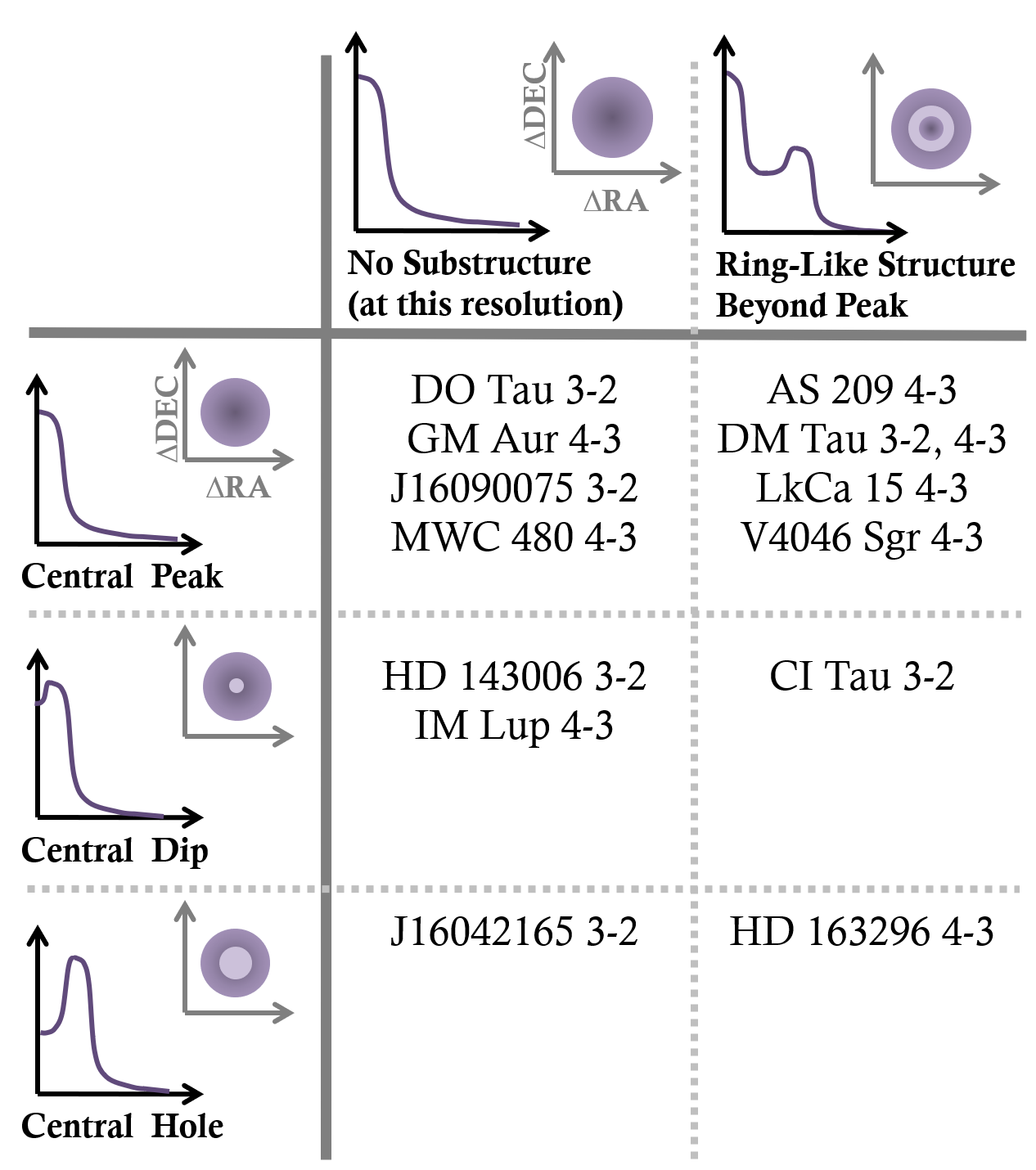
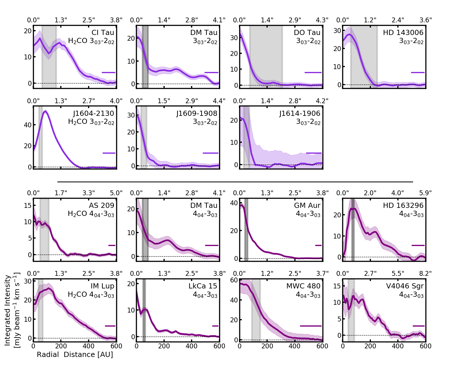
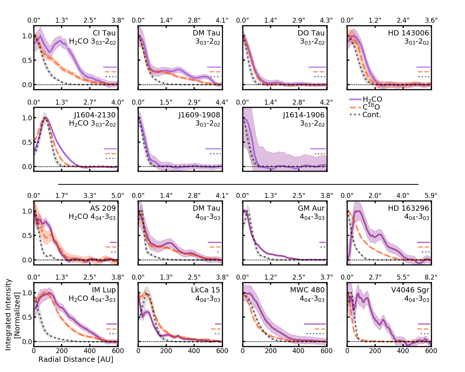
Figure 3 presents emission maps for all observed H2CO 303-202 and 404-303 lines, associated dust continuum, and C18O line emission. Figure 4 summarizes the emission morphologies of the disks detected in H2CO. Figure 5 shows the radial profiles of all H2CO 303-202 and 404-303 lines. We see a variety of H2CO spatial structures between the 13 detected disks. The majority (8/13) of the disks are centrally peaked in H2CO. Three disks have central dips (central depressions that are 1-3 deep) in H2CO, while the last two disks have central holes (central depressions that are 3 deep) in H2CO. About half (6/13) of the disks show outer rings or plateaus in H2CO emission. DM Tau, for example, has rings in its H2CO 404-303 emission and a plateau with suggestive ring-like substructure in its H2CO 303-202 emission.
Figure 6 compares the H2CO radial profiles with the dust continuum and C18O radial profiles. The majority (10/13) of the disks show H2CO emission beyond the edges of the dust continuum (defined as the radial extent at which the azimuthally-averaged continuum emission is 5% of its peak). Of the five disks that show inner holes in the dust continuum at our resolution, only one disk, J1604-2130, shows a similar inner hole in the H2CO emission. Dust and H2CO emission substructure thus do not necessarily coincide. The C18O and H2CO emission morphologies are more similar than the dust and H2CO: seven disks have similar radial extents in H2CO and C18O, and five have similar outer slopes in H2CO and C18O emission. However, there are also distinct differences between the H2CO and C18O emission morphologies, indicating that H2CO substructure is set by chemistry as well as by the disk gas distribution.
A priori, one possible explanation for the central H2CO depressions observed is dust opacity, i.e. optically thick dust blocking out molecular emission. C18O emission profiles provide an avenue to test this. We do see C18O depressions in three disks with H2CO inner dips or holes: IM Lup, J1604-2130, and LkCa 15 (Figure 6). However, for two of these disks (J1604-2130 and LkCa 15) the C18O depressions coincide with central holes in the dust continuum and are therefore explained by holes in gas and dust rather than by dust opacity. This leaves IM Lup as the only case where the central H2CO depression is likely due to dust opacity, at least in part. For all disks except IM Lup, optically thick dust is likely not a major cause for the H2CO emission substructure in the sample.
IV.3. Rotational Diagram Analysis

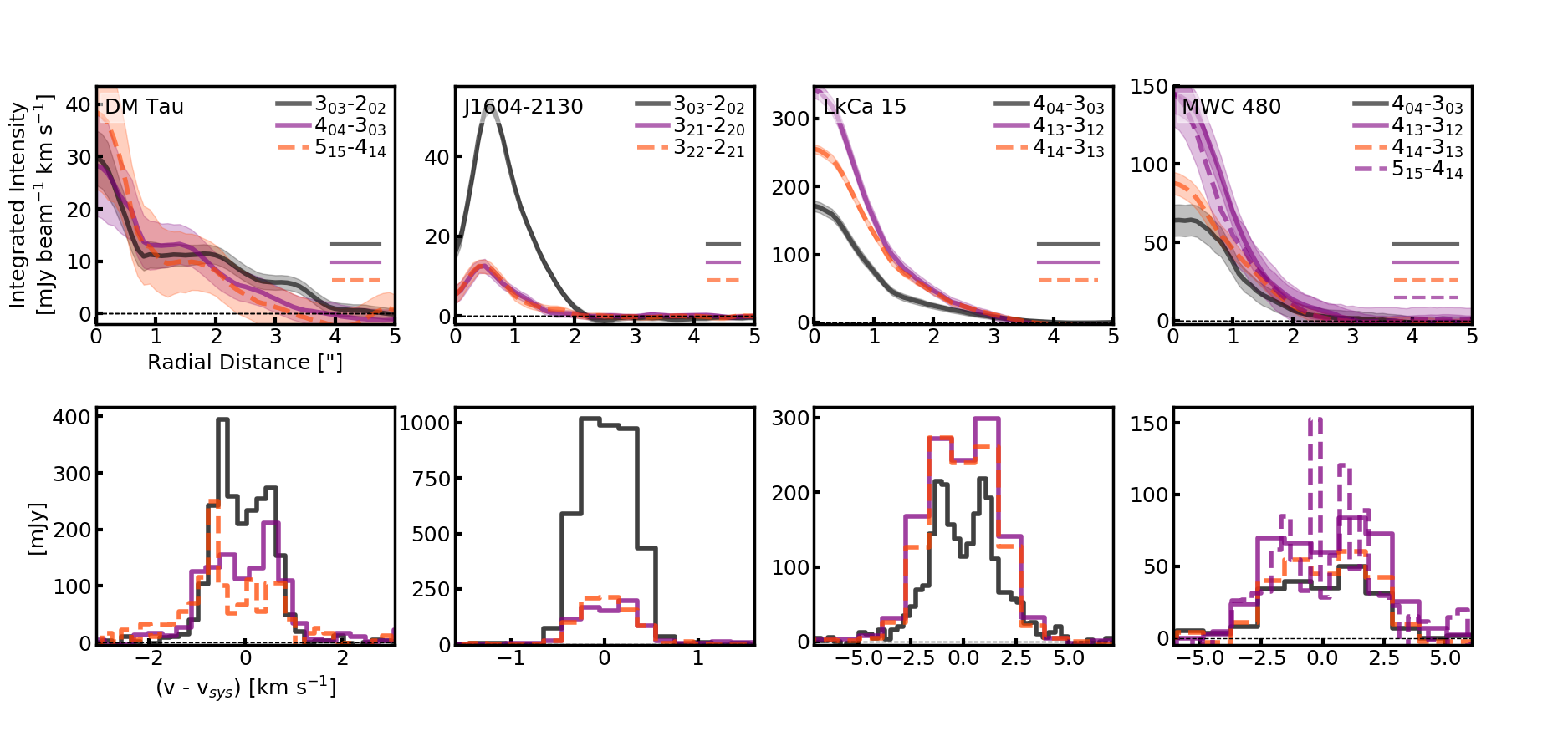
Three or more H2CO lines are detected towards four disks: DM Tau, J1604-2130, LkCa 15, and MWC 480. The velocity-integrated emission maps are shown in Figure 7, while the radial profiles and spectra are shown in Figure 8. For these four disks, we fit for the area-averaged H2CO excitation temperatures () and column densities () using the rotational diagram method (Blake et al. 1987; Goldsmith & Langer 1999, e.g.). This method assumes that the lines are in local thermodynamic equilibrium (LTE), that all lines originate from the same disk environment, and that the emission fills the beam. LTE should be a reasonable approximation, since the H2CO critical densities are lower than typical disk densities in the midplane and warm molecular disk layers (see Figure 1 in the Appendix). It is a reasonable first approximation that the emission fills the beam, since the H2CO emission is always resolved; however unresolved emission substructure may be present.
Following Loomis et al. 2018, we construct opacity-corrected rotational diagrams by relating and to the area-averaged column density and degeneracy of each line’s upper state:
| (1) |
where is the area-averaged column density if the line is actually optically thin, is the area-averaged velocity-integrated flux (in units of spectral flux density velocity), is the Einstein coefficient, and is the solid angle of area over which is averaged. Next, is the Planck constant, is the speed of light, is the partition function at temperature (Müller et al. 2005, interpolated from and values from CDMS;), and is the upper energy level. Finally, is the opacity correction factor (Goldsmith & Langer 1999, e.g.,), where the opacity of the line can be calculated as:
| (2) |
where , with accuracy within 99%, 95%, and 90% at of 0.6, 1.0, and 1.25 respectively. is the line frequency, is the Boltzmann constant, and is the intrinsic line width, assumed to be a combination of thermal and turbulent broadening (Flaherty et al. 2015, e.g.,):
| (3) |
where and are the masses of H2CO and H respectively, is the assumed mean molecular weight of the disk, and is the assumed prefactor for the turbulent contribution (Flaherty et al. 2015, e.g.,).
Combining Equations 1 and 2, we initially solve for the opacity-uncorrected and using a linear fit assuming , and then we correct the rotational diagram for the opacity using an iterative approach: (1) solve for each using Equation 2, (2) recalculate each using Equation 1, (3) redo the linear fit to the rotational diagram (the last line of Equation 1), and use the fit to (4) recalculate the values for and from the fit’s slope and y-intercept, respectively. We repeat this process until we reach convergence, defined as when the difference in the values and between two iterations is at most 0.001% (or, in the case of the uncertain spike in excitation temperature for LkCa 15, until 5000 iterations have passed).
| Disk | (H2CO Line) | ||
|---|---|---|---|
| [K] | [ cm-2] | ||
| DM Tau | (303-202), (404-303), (515-414) | ||
| J1604-2130 | (303-202), (321-220), (322-221) | ||
| LkCa 15 | (404-303), (413-312), (414-313) | ||
| MWC 480 | (404-303), (413-312), (414-313), (515-414) |
Note. — Values were derived from the linear fits of Figure 9. Errors and fits include 10% absolute flux uncertainties, added in quadrature to the velocity-integrated flux uncertainties.


Figure 9 displays the disk-averaged rotational diagrams. The disk area is measured out to where at least one H2CO line has azimuthally-averaged intensities above 1. Table 5 lists the extracted disk-averaged excitation temperatures and column densities. The disk-averaged excitation temperatures span 11-37K. The disk-averaged column densities span a little more than an order of magnitude: J1604-2130 has the largest column density at cm-2, while MWC 480 has the lowest at cm-2. Notably the energy ranges covered by the H2CO lines for each disk are similar, implying that these results are not due to excitation effects from using different H2CO lines.
For each disk we also construct azimuthally-averaged rotational diagrams. For each fit, we extract the integrated flux for each line from within the same narrow (0.1”) rings of the deprojected disk around the host star. We then construct a rotational diagram for each ring, assuming that each ring has uniform temperature and column density (see Loomis et al. 2018 for more details). Figure 10 displays the azimuthally-averaged excitation temperatures. In all disks except J1604-2130, the radially-resolved temperature profiles are close to consistent with a constant temperature. The excitation temperature increase towards J1604-2130 conincides with the inner dust edge, and may be due to direct radiation from the host star. Otherwise, the H2CO excitation temperature across disks are 20-50K, with the exception of DM Tau, where most H2CO appears to be at 10-15K. We note that DM Tau is an M-star with a massive disk, and it is therefore perhaps unsurprising that it hosts the coldest H2CO.
Figure 10 also displays the azimuthally-averaged H2CO column densities. The column density profiles generally vary between the four disks, closely following their H2CO line emission profiles. Notably the observed H2CO line emission plateau towards DM Tau seems to be due to a near-flat column density profile beyond 100 AU in this disk. Interestingly, H2CO has the smallest column density towards MWC 480, the only disk of these four that is irradiated by a Herbig Ae star.
IV.4. Radial H2CO Column Density Profiles across the Sample

For each disk where a single H2CO line was detected, we estimate a range of azimuthally-averaged column density profiles using Equation 1 for H2CO excitation temperatures between 20-50K. Figure 11 displays the resulting H2CO column density profiles, demonstrating that they are quite insensitive to excitation temperature assumptions in this range. Across the disks, estimated column densities span nearly three orders of magnitude, from cm-2. The highest column densities are seen at about 25 AU and 100 AU for the disks GM Aur and J1604-2130, respectively; notably, these locations are near the inner edges of the holes in the disks’ dust continuum. The lowest column densities are seen for the disks HD 163296, MWC 480, and V4046 Sgr, which present low column densities across their entire disks. Notably HD 163296 and MWC 480 are the only Herbig Ae disks in the sample, and V4046 Sgr is a very old disk.


Figure 12 plots the median radial H2CO column density profiles from Figure 11, grouped by stellar age on the left and stellar type (T Tauri or Herbig Ae) on the right. The right-hand panel of Figure 12 shows that the median Herbig Ae H2CO column densities are generally lower than the T Tauri medians. Note that this trend is tentative, since there are only two Herbig Ae disks in the sample, and there is overlap between the T Tauri and Herbig Ae distributions. The left-hand panel shows that the median H2CO column densities for the old disks (5Myr) are similar to the Herbig Ae medians, because both Herbig Ae disks are 5Myr. However, given that the 5Myr disk J1604-2130 hosts some of the largest H2CO column densities in the survey, it seems more likely that the tentative trend is explained by stellar type rather than stellar age. There is no trend in H2CO column density with dust continuum size (not shown).
V. Discussion
V.1. H2CO Formation Chemistry
Interpretations of our observed H2CO morphologies and profiles rely on an understanding of the possible astrochemical origins of H2CO in disks, which we briefly review here.
Astrochemical laboratory experiments and models have shown that H2CO can form efficiently from both gas-phase and grain-surface chemistry. In the gas phase, H2CO can form through multiple pathways, including the neutral-neutral reaction (Fockenberg & Preses 2002; Atkinson et al. 2006, e.g.):
CH3 + O H2CO + H
Under laboratory conditions from 290-930K, the H2CO yield from this reaction is roughly constant (Fockenberg & Preses 2002, e.g.,). Astrochemical disk modeling has shown that at low temperatures (100K), this pathway is the dominant source of gas-phase H2CO formation (van der Marel et al. 2014; Loomis et al. 2015), and that gas-phase production of H2CO in general is most efficient in the warm, dense inner regions of the disk (Loomis et al. 2015).
On grain surfaces, H2CO can form through the sequential hydrogenation of CO ice, which also produces CH3OH if the hydrogenation continues (Hiraoka et al. 1994; Hiraoka et al. 2002; Watanabe & Kouchi 2002; Hidaka et al. 2004; Watanabe et al. 2004; Fuchs et al. 2009, e.g.):
CO HCO H2CO H2COH CH3OH
We expect CO hydrogenation to produce H2CO efficiently beyond the CO snowline. However, since H2CO grain-surface production is possible as long as some CO is on the grains long enough to react with atomic hydrogen, H2CO grain-surface production likely also occurs somewhat interior to the CO snowline (Öberg et al. 2017).
H2CO is less volatile than CO; the desorption energies of H2CO off of different icy surfaces range from 3300-3700K (Noble et al. 2012), while the desorption energies of 13CO range from 900-1600K (Fayolle et al. 2016). Therefore H2CO freezes out at temperatures higher than 80K, which is interior to the CO snowline at smaller radial distances in the disks than we are sensitive to. However, frozen-out H2CO beyond the H2CO snowline can still be released into the gas via non-thermal desorption (Walsh et al. 2014; Loomis et al. 2015; Öberg et al. 2017; Féraud et al. 2019, e.g.).
V.2. H2CO and the CO Snowline
| Disk | CO Midpl. | Reference |
|---|---|---|
| Snowline | ||
| Range | ||
| [AU] | ||
| AS 209 | 50-111 | Bergner et al. 2019 |
| CI Tau | 64-166 | Bergner et al. 2019 |
| DM Tau | 45-85 | Qi et al. 2019 |
| DO Tau | 76-310 | Bergner et al. 2019 |
| GM Aur | 40-58 | Qi et al. 2019 |
| HD 143006 | 59-251 | Bergner et al. 2019 |
| HD 163296 | 69-83 | Qi et al. 2015 |
| IM Lup | 38-69 | Bergner et al. 2019 |
| J1604-2130 | 43-64 | Bergner et al. 2019 |
| J1609-1908 | 36-73 | Bergner et al. 2019 |
| J1612-1859 | 36-78 | Bergner et al. 2019 |
| J1614-1906 | 31-71 | Bergner et al. 2019 |
| LkCa 15 | 48-64 | Qi et al. 2019 |
| MWC 480 | 90-150∗ | Loomis et al. (subm.) |
| V4046 Sgr | 40-85 | Bergner et al. 2019 |
Note. — All locations have been scaled to new GAIA distances (Table 1). : The CO snowline was estimated as 120 AU by Loomis et al. (subm.); here we broaden the snowline by 30 AU to account for the resolution of the data.
To constrain H2CO formation pathways in our survey, we compare the observed H2CO emission profiles with estimated locations of CO snowlines at the disk midplane. Studies have inferred CO snowlines for disks using CO isotopologues and chemical tracers of CO freeze-out, and found freeze-out temperatures between 17-26K (Mathews et al. 2013; Qi et al. 2013; Qi et al. 2015; Öberg et al. 2015a; Schwarz et al. 2016; Pinte et al. 2018, e.g.). For DM Tau, GM Aur, HD 163296, and LkCa 15, we use the CO snowline locations fitted using N2H+ as a tracer by Qi et al. 2015 and Qi et al. 2019. For the nine other disks with detected H2CO, we estimate midplane snowlines at locations corresponding to a similar temperature range of 17-25K, extracted from the disk toy models of Bergner et al. 2019 and Loomis et al. (subm.). Note that these model-based estimates are very uncertain, and in at least two cases (AS 209 and V4046 Sgr) they overestimate the CO snowline location compared to the location based on N2H+ (Qi et al. 2019). Three disks DO Tau, HD 143006, and J1609-1908 have CO snowline ranges that are too broad to be informative, and we exclude them from further analysis.
Figure 5 compares the H2CO profiles and the inferred CO snowline locations. There is significant H2CO emission both interior and exterior to the CO snowline of all disks. A majority (6/10) of the H2CO radial profiles peak interior to the CO snowline, but have rings or plateaus in H2CO at or beyond the CO snowline. Two of the remaining disks, IM Lup and J1604-2130, have H2CO radial profiles that peak beyond the CO snowline. One of the last two disks, MWC 480, may show more substructure at higher resolution. The simplest explanation for these H2CO morphologies is that H2CO is produced through both gas-phase and grain-surface chemistry in disks. The substantial central H2CO emission found interior to the CO snowline implies an inner component of H2CO produced in the gas phase and/or due to sublimation of inward-moving grains. The rings and local enhancements in H2CO emission found at or beyond the CO snowline are best explained by grain-surface production, since the efficiency of H2CO gas-phase formation is expected to decrease with disk radius.
It is possible that H2CO ices inherited from the preceding protostellar stage are contributing to the observed H2CO emission in disks. While we would expect inherited H2CO ices to mainly contribute to emission in the inner disk, where H2CO desorption would be efficient, we cannot exclude a smaller contribution in the outer disk, which may arise from the mixing of midplane ices into the warm upper layers of the disk. However, there should be no relationship between this emission and the CO snowline, which suggests that inheritance alone cannot explain the observed H2CO emission morphologies.
Our results thus indicate that the two-component H2CO model discussed by Loomis et al. 2015, Carney et al. 2017, and Öberg et al. 2017 for three specific disks, containing one warm inner component and one cold component exterior to the CO snowline, likely holds for disks generally. Furthermore, it is likely that H2CO is commonly produced through both gas-phase and grain-surface chemistry in disks.
We expect that the H2CO formed through CO hydrogenation beyond the CO snowline will coincide with the formation of complex oxygen-bearing organics, particularly methanol (CH3OH), as these molecules can form along the same hydrogenation pathway as H2CO (Hiraoka et al. 1994; Watanabe & Kouchi 2002, e.g.,). However, since there is also some contribution from gas-phase chemistry to the total H2CO budget at these radii, it is difficult to assess how much of these COMs are present. Detailed modeling, as well as a few benchmarking disks with both H2CO and COM detections, are needed to quantify the relationship between H2CO and COM production in disks. In the meantime, we conclude that a majority of disks do have an active organic ice chemistry, and that COM production should be expected in the outer regions of most protoplanetary disks.
The exception to this conclusion may be disks around Herbig Ae stars, because their warmer temperatures allow for limited CO freeze-out. Our survey tentatively shows that T Tauri disks have more H2CO than Herbig Ae disks, despite how the Herbig Ae disks present the highest C18O flux densities. This finding is consistent with the single-dish survey of H2CO in disks conducted by Guilloteau et al. 2013, which showed that warmer disks tended to have less H2CO emission. It is also consistent with the Submillimeter Array (SMA) survey conducted by Öberg et al. 2010, which noted that the lower detection rates towards Herbig Ae disks could be because their midplanes are too warm for a cold CO-ice based chemistry. Therefore our results could be explained by a small or non-existing production of H2CO through CO ice hydrogenation in Herbig Ae disks. More spatially-resolved observations of H2CO towards Herbig Ae disks are needed to further evaluate this tentative trend.
V.3. Relationship between H2CO and Dust Substructure
Carney et al. 2017 and Öberg et al. 2017 note three ways that H2CO could be affected by a hole or edge in the dust continuum: (1) through enhanced temperatures due to greater irradiation in regions with fewer solids (Cleeves et al. 2011; Cleeves 2016); (2) through increased photodesorption of H2CO off the grains from the increased irradiation (Öberg et al. 2015a); and/or (3) through increased CO photodissociation in the upper layers, since more CO in the upper layers could produce more hydrocarbon radicals and atomic oxygen in the gas, and then possibly allow for more efficient gas-phase production of H2CO (Carney et al. 2017; Öberg et al. 2017). Five of the disks in our survey (DM Tau, GM Aur, J1604-2130, LkCa 15, and V4046 Sgr) have inner holes in the submillimeter/millimeter dust continuum that are detected at our spatial resolution. For these five disks, we see no universal trend in H2CO emission morphologies in the inner disks. Four of the five disks show centrally-peaked H2CO emission despite the central depletions in dust continuum. The final disk, J1604-2130, does show an inner hole in the H2CO emission. Notably J1604-2130 also has a large inner hole in its C18O emission (Zhang et al. 2014; van der Marel et al. 2015, see also). We also do not see a consistent trend in H2CO emission morphologies at the outer dust continuum edges, but four of the disks show clear bumps in H2CO emission right at those edges. It therefore appears that, while dust substructure does influence the distribution of H2CO in disks, there is no single relationship between the two.
V.4. H2CO Excitation Temperatures
The H2CO excitation temperature should reflect the temperature of the vertical layer in the disk within which the gas resides, as long as the densities are high enough for LTE. T Tauri disk models predict that beyond 50 AU (the scale we are most sensitive to), the midplane will be 10-30K, the molecular layer 20-50K, and the atmosphere 50-500K (Walsh et al. 2010, e.g.,). Herbig Ae disks will have warmer temperatures at the same radial distances, while low-mass M-star disks will have colder temperatures. In the four disks where we could measure H2CO excitation temperatures, three are consistent with the warm molecular layer, and one (DM Tau) with the disk midplane, indicating that the vertical distribution of H2CO may vary between disks.
Our radially-resolved rotational diagram analysis is largely consistent with a constant radial temperature per disk in the outer disks beyond 100-200 AU. This suggests that for three of the four disks, H2CO is consistently emitting from the molecular layer at/above CO freeze-out temperatures. This is in accordance with model predictions, which find the most abundant H2CO in the molecular layer above 20K (Walsh et al. 2010). However, since error bars are currently large (typically 10K or more), we need more precise observations in order to better constrain radial H2CO excitation temperatures.
VI. Summary
We have conducted an ALMA survey of H2CO towards 15 protoplanetary disks. We have analyzed the H2CO morphologies, excitation temperatures, and column densities, and their relationships to stellar and disk characteristics. We summarize our main findings below:
- 1.
We report a total of 26 H2CO detections towards 13/15 disks, consisting of one line towards 8 disks, two lines towards 1 disk, three lines towards 2 disks, four lines towards 1 disk, and six lines towards 1 disk. We report an additional 11 tentative H2CO detections across 7/15 disks.
- 2.
Over half of the disks have centrally-peaked H2CO emission, while the rest have central dips or holes in H2CO emission. About half of the disks show rings or a plateau in H2CO emission in the outer disk.
- 3.
We measure disk-averaged and azimuthally-averaged H2CO excitation temperatures for four disks with multiple H2CO line detections. Three of the four disks have disk-averaged excitation temperatures of 21-37K, while the fourth disk, DM Tau, is colder at 11K. The azimuthally-averaged temperatures show an increase at the inner dust edge of J1604-2130, but otherwise close to constant radial temperatures for the disks.
- 4.
In addition to the disks we could directly model, we estimate radial H2CO column densities for all disks assuming excitation temperatures of 20-50K. The column densities between and across the disks of our survey span three orders of magnitude, from . The highest H2CO column densities are found near the inner dust continuum edges of the disks GM Aur and J1604-2130. The lowest H2CO column densities are found across the Herbig Ae disks HD 163296 and MWC 480, as well as in the old disk V4046 Sgr.
- 5.
Based on simple estimates of CO midplane snowline locations, significant H2CO emission is present both interior and exterior to the CO snowline in all disks, with ring-like structures in the emission occurring beyond the CO snowline in half of the disks. This suggests that H2CO is commonly formed through both gas-phase and grain-surface pathways in protoplanetary disks, and that a majority of disks present an active organic ice chemistry that is likely also producing COMs. The low H2CO column densities toward the two Herbig Ae disks in the sample may be due to a smaller degree of CO ice chemistry in these warmer disks.
- •
ADS/JAO.ALMA#2011.0.00629.S
- •
ADS/JAO.ALMA#2012.1.00681.S
- •
ADS/JAO.ALMA#2013.1.00226.S
- •
ADS/JAO.ALMA#2015.1.00657.S
- •
ADS/JAO.ALMA#2015.1.00678.S
- •
ADS/JAO.ALMA#2015.1.00964.S
- •
ADS/JAO.ALMA#2016.1.00627.S.
ALMA is a partnership of ESO (representing its member states), NSF (USA) and NINS (Japan), together with NRC (Canada), MOST and ASIAA (Taiwan), and KASI (Republic of Korea), in cooperation with the Republic of Chile. The Joint ALMA Observatory is operated by ESO, AUI/NRAO and NAOJ. The National Radio Astronomy Observatory is a facility of the National Science Foundation operated under cooperative agreement by Associated Universities, Inc.
This work has made use of data from the European Space Agency (ESA) mission Gaia (https://www.cosmos.esa.int/gaia), processed by the Gaia Data Processing and Analysis Consortium (DPAC, https://www.cosmos.esa.int/web/gaia/dpac/consortium). Funding for the DPAC has been provided by national institutions, in particular the institutions participating in the Gaia Multilateral Agreement.
All computer code used for this research was written in Python (version 2.7). All plots were generated using Python’s Matplotlib package (Hunter 2007). This research also made use of Astropy (http://www.astropy.org), a community-developed core Python package for Astronomy, and the NumPy (Oliphant 2006–) and SciPy (Jones et al. 2001–) Python packages.
Fig. Set A1. Channel maps of detected H2CO 303-202 and 404-303 above 2.
Fig. Set A2. Channel maps of detected C18O above 2.
Fig. Set A3. Channel maps of all detected H2CO lines (other than 303-202 and 404-303) above 2.
| Disk | Position | Inclination | H2CO and Cont. | C18O | Systemic |
|---|---|---|---|---|---|
| Angle∗ | Angle∗ | Mask Radius∗∗ | Mask Radius∗∗ | Velocity | |
| [∘] | [∘] | [”] | [”] | [km s-1] | |
| AS 209 | 6.6 | 31.2 | 2.0 | 2.9 | 4.600 |
| CI Tau | 260.4 | 41.6 | 3.4 | 4.7 | 5.840 |
| DM Tau | 110.3 | 23.2 | 4.0 | 4.1 | 6.070 |
| DO Tau | 113.4 | 18.5 | 3.5 | 2.3 | 5.900 |
| GM Aur | 33.8 | 37.2 | 2.7 | - | 5.550 |
| HD 143006 | 277.1 | 24.0 | 1.7 | 1.7 | 7.755 |
| HD 163296 | 136.9 | 43.7 | 4.8 | 4.1 | 5.790 |
| IM Lup | 305.3 | 46.2 | 3.4 | 3.4 | 4.400 |
| J1604-2130 | 194.6 | 6.2 | 2.3 | 2.0 | 4.600 |
| J1609-1908 | 103.4 | 32.1 | 1.7 | - | 3.800 |
| J1612-1859 | 151.9 | 30.9 | 0.8 | - | 4.700 |
| J1614-1906 | 262.5 | 40.9 | 0.8 | - | 3.800 |
| LkCa 15 | 33.1 | 37.8 | 4.0 | 4.1 | 6.300 |
| MWC 480 | 122 | 37.4 | 3.6 | 5.0 | 5.100 |
| V4046 Sgr | 191.9 | 29.3 | 5.6 | 4.0 | 2.900 |
Note. — All Keplerian masks were generated assuming the combined thermal and turbulent line width is (Yen et al. 2016). For all disks, we fixed and to be 100 AU and -0.3, respectively. For most disks, we fixed to be 0.3km s-1. The exceptions were the broader H2CO 414-313 and 413-312 lines, for which we fixed to be 0.6km s-1, as well as the nearly face-on disk J1604-2130, for which we fixed to be 0.15km s-1. ∗: The position and inclination angles were estimated using a grid-search algorithm and the fixed broadening parameters. We stress that these estimates are not exact measurements of the disk angles. They are parametric values used only to maximize the masked emission. : The Keplerian mask radii were set where the azimuthally-averaged emission intensities first reached zero. For disks with multiple H2CO lines observed, we used the same (largest) mask radius for all lines to maintain a consistent area of H2CO emission.
| Disk | Size∗ | Sum∗∗ | Peak Em.∗∗ | rms ()† | Beam Size (P.A.) | |
|---|---|---|---|---|---|---|
| [mm] | [AU] | [mJy] | [mJy beam-1] | [mJy beam-1] | ||
| AS 209 | 1.0 | 66.5 | 297 | 45 | 0.18 | 0.31” x 0.21” (-70.80 deg) |
| CI Tau | 1.3 | 206.7 | 161 | 54 | 0.16 | 0.63” x 0.44” (30.36 deg) |
| DM Tau | 1.3 | 159.5 | 99 | 37 | 0.10 | 0.60” x 0.44” (35.26 deg) |
| 1.0 | 65.2 | 89 | 8.7 | 0.15 | 0.18” x 0.15” (14.33 deg) | |
| 0.9 | 159.5 | 224 | 91 | 0.31 | 0.65” x 0.44” (-28.59 deg) | |
| DO Tau | 1.3 | 98.0 | 127 | 102 | 0.27 | 0.68” x 0.44” (29.50 deg) |
| GM Aur | 1.0 | 79.5 | 255 | 26 | 0.13 | 0.29” x 0.19” (-1.65 deg) |
| HD 143006 | 1.3 | 148.5 | 53 | 21 | 0.12 | 0.69” x 0.47” (-75.15 deg) |
| HD 163296 | 1.0 | 121.2 | 956 | 219 | 0.87 | 0.44” x 0.33” (-84.74 deg) |
| IM Lup | 1.0 | 189.6 | 237 | 78 | 0.35 | 0.40” x 0.33” (78.16 deg) |
| J1604-2130 | 1.3 | 178.8 | 69 | 11 | 0.14 | 0.63” x 0.43” (-77.99 deg) |
| J1609-1908 | 1.3 | 95.9 | 22 | 18 | 0.14 | 0.63” x 0.43” (-76.80 deg) |
| J1612-1859 | 1.3 | 96.6 | 3.6 | 3.0 | 0.13 | 0.63” x 0.43” (-76.23 deg) |
| J1614-1906 | 1.3 | 100.1 | 19 | 17 | 0.14 | 0.62” x 0.43” (-76.99 deg) |
| LkCa 15 | 1.0 | 94.8 | 281 | 23 | 0.11 | 0.32” x 0.26” (-17.58 deg) |
| MWC 480 | 1.0 | 209.3 | 482 | 347 | 0.27 | 1.05” x 0.84” (-5.72 deg) |
| 0.9 | 161.0 | 848 | 448 | 0.44 | 0.78” x 0.42” (-23.28 deg) | |
| V4046 Sgr | 1.0 | 80.3 | 542 | 75 | 0.18 | 0.50” x 0.39” (-70.09 deg) |
Note. — : The radial extent of the dust continuum is defined as where the continuum emission is 5% of its peak. : The fluxes and peak fluxes were measured within the same Keplerian mask radii used for H2CO (Table 1). Errors are small relative to the fluxes. : The average rms across 1000 1”-by-1” random samples, extracted 3”-7” away from the disk center.
| Disk | Flux∗ | Peak Flux∗ | Int. Vel. | Chan. | Chan. | Beam Size (P.A.) |
|---|---|---|---|---|---|---|
| [mJy | [mJy beam-1 | Range | Width | rms∗∗ | ||
| km s-1] | km s-1] | [km s-1] | [km s-1] | [mJy beam-1] | ||
| AS 209 | 429 30 | 53 6.4 | 0.9 - 8.1 | 0.4 | 8.0 | 0.53” x 0.50” (37.32∘) |
| CI Tau | 549 17 | 44 3.3 | 2.6 - 9.0 | 0.2 | 5.4 | 0.67” x 0.46” (31.32∘) |
| DM Tau | 998 17 | 66 3.2 | 3.6 - 8.6 | 0.2 | 5.6 | 0.63” x 0.47” (36.01∘) |
| DO Tau | 210 12 | 82 3.6 | 3.2 - 8.8 | 0.2 | 5.3 | 0.72” x 0.46” (30.42∘) |
| HD 143006 | 135 10 | 43 3.6 | 5.4 - 10.2 | 0.2 | 5.5 | 0.70” x 0.48” (-79.98∘) |
| HD 163296 | 5040 31 | 355 6.7 | -1.4 - 13.0 | 0.2 | 4.9 | 0.61” x 0.52” (62.26∘) |
| IM Lup | 1203 14 | 80 4.1 | 0.2 - 8.6 | 0.2 | 4.9 | 0.58” x 0.43” (-64.43∘) |
| J1604-2130 | 1267 7.2 | 141 1.7 | 3.7 - 5.5 | 0.2 | 5.4 | 0.65” x 0.45” (-80.59∘) |
| LkCa 15 | 619 18 | 53 3.7 | 2.3 - 10.3 | 0.2 | 4.7 | 0.55” x 0.43” (11.85∘) |
| MWC 480 | 1648 20 | 290 11 | -1.0 - 11.2 | 0.2 | 4.6 | 0.64” x 0.41” (13.23∘) |
| V4046 Sgr | 1184 18 | 385 5.1 | -4.3 - 10.1 | 0.2 | 4.5 | 0.73” x 0.49” (89.68∘) |
Note. — *: The velocity-integrated fluxes (Column 2) were measured within the bounds of the Keplerian masks (Table 1). The peak fluxes (Column 3) are the peaks of the velocity-integrated emission maps; note the difference in unit compared to the velocity-integrated fluxes. The uncertainty in each peak flux is the standard deviation of the peaks across 1000 random samples. Uncertainties do not include absolute flux uncertainties. : The channel rms was estimated as the standard deviation of 1000 1”-by-1” random samples.

References
- Aikawa et al. (2003) Aikawa, Y., Momose, M., Thi, W.-F., et al. 2003, PASJ, 55, 11
- Andrews et al. (2018) Andrews, S. M., Huang, J., Pérez, L. M., et al. 2018, ApJ, 869, L41
- Atkinson et al. (2006) Atkinson, R., Baulch, D. L., Cox, R. A., et al. 2006, Atmospheric Chemistry and Physics, 6, 3625. https://www.atmos-chem-phys.net/6/3625/2006/
- Bergin et al. (2004) Bergin, E., Calvet, N., Sitko, M. L., et al. 2004, ApJ, 614, L133
- Bergner et al. (2018) Bergner, J. B., Guzmán, V. G., Öberg, K. I., Loomis, R. A., & Pegues, J. 2018, ApJ, 857, 69
- Bergner et al. (2019) Bergner, J. B., Öberg, K. I., Bergin, E. A., et al. 2019, ApJ, 876, 25
- Blake et al. (1987) Blake, G. A., Sutton, E. C., Masson, C. R., & Phillips, T. G. 1987, ApJ, 315, 621
- Boogert et al. (2008) Boogert, A. C. A., Pontoppidan, K. M., Knez, C., et al. 2008, ApJ, 678, 985
- Carney et al. (2017) Carney, M. T., Hogerheijde, M. R., Loomis, R. A., et al. 2017, A&A, 605, A21
- Chapillon et al. (2012) Chapillon, E., Dutrey, A., Guilloteau, S., et al. 2012, ApJ, 756, 58
- Cleeves (2016) Cleeves, L. I. 2016, ApJ, 816, L21
- Cleeves et al. (2011) Cleeves, L. I., Bergin, E. A., Bethell, T. J., et al. 2011, ApJ, 743, L2
- Condon & Ransom (2016) Condon, J. J., & Ransom, S. M. 2016, Spectral Lines (The National Radio Astronomy Observatory)
- Cridland et al. (2016) Cridland, A. J., Pudritz, R. E., & Alessi, M. 2016, MNRAS, 461, 3274
- Cridland et al. (2017) Cridland, A. J., Pudritz, R. E., Birnstiel, T., Cleeves, L. I., & Bergin, E. A. 2017, arXiv e-prints, arXiv:1705.02381
- Drozdovskaya et al. (2019) Drozdovskaya, M. N., van Dishoeck, E. F., Rubin, M., Jørgensen, J. K., & Altwegg, K. 2019, MNRAS, 490, 50
- Drozdovskaya et al. (2014) Drozdovskaya, M. N., Walsh, C., Visser, R., Harsono, D., & van Dishoeck, E. F. 2014, MNRAS, 445, 913
- Dutrey et al. (1997) Dutrey, A., Guilloteau, S., & Guelin, M. 1997, A&A, 317, L55
- Endres et al. (2016) Endres, C. P., Schlemmer, S., Schilke, P., Stutzki, J., & Müller, H. S. P. 2016, Journal of Molecular Spectroscopy, 327, 95
- Espaillat et al. (2010) Espaillat, C., D’Alessio, P., Hernández, J., et al. 2010, ApJ, 717, 441
- Favre et al. (2018) Favre, C., Fedele, D., Semenov, D., et al. 2018, ApJ, 862, L2
- Fayolle et al. (2016) Fayolle, E. C., Balfe, J., Loomis, R., et al. 2016, ApJ, 816, L28
- Flaherty et al. (2015) Flaherty, K. M., Hughes, A. M., Rosenfeld, K. A., et al. 2015, ApJ, 813, 99
- Fockenberg & Preses (2002) Fockenberg, C., & Preses, J. M. 2002, The Journal of Physical Chemistry A, 106, 2924. http://dx.doi.org/10.1021/jp0141880
- Fuchs et al. (2009) Fuchs, G. W., Cuppen, H. M., Ioppolo, S., et al. 2009, A&A, 505, 629
- Féraud et al. (2019) Féraud, G., Bertin, M., Romanzin, C., et al. 2019, ACS Earth and Space Chemistry
- Gaia Collaboration et al. (2018) Gaia Collaboration, Brown, A. G. A., Vallenari, A., et al. 2018, ArXiv e-prints, arXiv:1804.09365
- Gaia Collaboration et al. (2016a) Gaia Collaboration, Prusti, T., de Bruijne, J. H. J., et al. 2016a, A&A, 595, A1
- Gaia Collaboration et al. (2016b) Gaia Collaboration, Brown, A. G. A., Vallenari, A., et al. 2016b, A&A, 595, A2
- Gibb et al. (2004) Gibb, E. L., Whittet, D. C. B., Boogert, A. C. A., & Tielens, A. G. G. M. 2004, ApJS, 151, 35
- Goldsmith & Langer (1999) Goldsmith, P. F., & Langer, W. D. 1999, ApJ, 517, 209
- Guilloteau et al. (2013) Guilloteau, S., Di Folco, E., Dutrey, A., et al. 2013, A&A, 549, A92
- Guzmán et al. (2018) Guzmán, V. V., Öberg, K. I., Carpenter, J., et al. 2018, ApJ, 864, 170
- Henning & Semenov (2013) Henning, T., & Semenov, D. 2013, Chemical Reviews, 113, 9016
- Herbst & van Dishoeck (2009) Herbst, E., & van Dishoeck, E. F. 2009, ARA&A, 47, 427
- Hidaka et al. (2004) Hidaka, H., Watanabe, N., Shiraki, T., Nagaoka, A., & Kouchi, A. 2004, ApJ, 614, 1124
- Hiraoka et al. (1994) Hiraoka, K., Ohashi, N., Kihara, Y., et al. 1994, Chemical Physics Letters, 229, 408 . http://www.sciencedirect.com/science/article/pii/0009261494010668
- Hiraoka et al. (2002) Hiraoka, K., Sato, T., Sato, S., et al. 2002, ApJ, 577, 265
- Huang et al. (2017) Huang, J., Öberg, K. I., Qi, C., et al. 2017, ApJ, 835, 231
- Hunter (2007) Hunter, J. D. 2007, Computing In Science & Engineering, 9, 90
- Jensen & Mathieu (1997) Jensen, E. L. N., & Mathieu, R. D. 1997, AJ, 114, 301
- Jones et al. (2001–) Jones, E., Oliphant, T., Peterson, P., et al. 2001–, SciPy: Open source scientific tools for Python, , . http://www.scipy.org/
- Kastner et al. (2018) Kastner, J. H., Qi, C., Dickson-Vandervelde, D. A., et al. 2018, ApJ, 863, 106
- Lee et al. (2019) Lee, J.-E., Lee, S., Baek, G., et al. 2019, Nature Astronomy, 3, 314
- Loomis et al. (2018) Loomis, R. A., Cleeves, L. I., Öberg, K. I., et al. 2018, ArXiv e-prints, arXiv:1805.01458
- Loomis et al. (2015) Loomis, R. A., Cleeves, L. I., Öberg, K. I., Guzman, V. V., & Andrews, S. M. 2015, ApJ, 809, L25
- Marsh & Mahoney (1992) Marsh, K. A., & Mahoney, M. J. 1992, ApJ, 395, L115
- Mathews et al. (2012) Mathews, G. S., Williams, J. P., Ménard, F., et al. 2012, ApJ, 745, 23
- Mathews et al. (2013) Mathews, G. S., Klaassen, P. D., Juhász, A., et al. 2013, A&A, 557, A132
- Mordasini et al. (2008) Mordasini, C., Alibert, Y., Benz, W., & Naef, D. 2008, in Astronomical Society of the Pacific Conference Series, Vol. 398, Extreme Solar Systems, ed. D. Fischer, F. A. Rasio, S. E. Thorsett, & A. Wolszczan, 235
- Müller et al. (2005) Müller, H. S. P., Schlöder, F., Stutzki, J., & Winnewisser, G. 2005, Journal of Molecular Structure, 742, 215
- Mumma & Charnley (2011) Mumma, M. J., & Charnley, S. B. 2011, ARA&A, 49, 471
- Noble et al. (2012) Noble, J. A., Theule, P., Mispelaer, F., et al. 2012, A&A, 543, A5
- Öberg & Bergin (2016) Öberg, K. I., & Bergin, E. A. 2016, ApJ, 831, L19
- Öberg et al. (2015a) Öberg, K. I., Furuya, K., Loomis, R., et al. 2015a, ApJ, 810, 112
- Öberg et al. (2015b) Öberg, K. I., Guzmán, V. V., Furuya, K., et al. 2015b, Nature, 520, 198
- Öberg et al. (2010) Öberg, K. I., Qi, C., Fogel, J. K. J., et al. 2010, ApJ, 720, 480
- Öberg et al. (2011) —. 2011, ApJ, 734, 98
- Öberg et al. (2017) Öberg, K. I., Guzmán, V. V., Merchantz, C. J., et al. 2017, ApJ, 839, 43
- Oliphant (2006–) Oliphant, T. 2006–, NumPy: A guide to NumPy, USA: Trelgol Publishing, , . http://www.numpy.org/
- Pinte et al. (2018) Pinte, C., Ménard, F., Duchêne, G., et al. 2018, A&A, 609, A47
- Podio et al. (2019) Podio, L., Bacciotti, F., Fedele, D., et al. 2019, A&A, 623, L6
- Pontoppidan et al. (2004) Pontoppidan, K. M., van Dishoeck, E. F., & Dartois, E. 2004, A&A, 426, 925
- Qi et al. (2015) Qi, C., Öberg, K. I., Andrews, S. M., et al. 2015, ApJ, 813, 128
- Qi et al. (2013) Qi, C., Öberg, K. I., & Wilner, D. J. 2013, ApJ, 765, 34
- Qi et al. (2019) Qi, C., Öberg, K. I., Espaillat, C. C., et al. 2019, ApJ, 882, 160
- Quast et al. (2000) Quast, G. R., Torres, C. A. O., de La Reza, R., da Silva, L., & Mayor, M. 2000, in IAU Symposium, Vol. 200, IAU Symposium, 28
- Rosenfeld et al. (2013) Rosenfeld, K. A., Andrews, S. M., Hughes, A. M., Wilner, D. J., & Qi, C. 2013, ApJ, 774, 16
- Rosenfeld et al. (2012) Rosenfeld, K. A., Andrews, S. M., Wilner, D. J., & Stempels, H. C. 2012, ApJ, 759, 119
- Salinas et al. (2017) Salinas, V. N., Hogerheijde, M. R., Mathews, G. S., et al. 2017, A&A, 606, A125
- Schwarz et al. (2016) Schwarz, K. R., Bergin, E. A., Cleeves, L. I., et al. 2016, ApJ, 823, 91
- Thi et al. (2004) Thi, W.-F., van Zadelhoff, G.-J., & van Dishoeck, E. F. 2004, A&A, 425, 955
- van der Marel et al. (2015) van der Marel, N., van Dishoeck, E. F., Bruderer, S., Pérez, L., & Isella, A. 2015, A&A, 579, A106
- van der Marel et al. (2014) van der Marel, N., van Dishoeck, E. F., Bruderer, S., & van Kempen, T. A. 2014, A&A, 563, A113
- van ’t Hoff et al. (2018) van ’t Hoff, M. L. R., Tobin, J. J., Trapman, L., et al. 2018, ApJ, 864, L23
- Walsh et al. (2010) Walsh, C., Millar, T. J., & Nomura, H. 2010, ApJ, 722, 1607
- Walsh et al. (2014) Walsh, C., Millar, T. J., Nomura, H., et al. 2014, A&A, 563, A33
- Walsh et al. (2016) Walsh, C., Loomis, R. A., Öberg, K. I., et al. 2016, ApJ, 823, L10
- Watanabe & Kouchi (2002) Watanabe, N., & Kouchi, A. 2002, ApJ, 571, L173
- Watanabe et al. (2004) Watanabe, N., Nagaoka, A., Shiraki, T., & Kouchi, A. 2004, ApJ, 616, 638
- Yen et al. (2016) Yen, H.-W., Koch, P. M., Liu, H. B., et al. 2016, ApJ, 832, 204
- Zhang et al. (2014) Zhang, K., Isella, A., Carpenter, J. M., & Blake, G. A. 2014, ApJ, 791, 42