Certified Defense to Image Transformations via Randomized Smoothing

Marc Fischer Maximilian Baader Martin Vechev Affiliation: Department of Computer Science Affiliation: ETH Zurich Affiliation: {marc.fischer, mbaader, martin.vechev}@inf.ethz.ch

Abstract

We extend randomized smoothing to cover parameterized transformations (e.g., rotations, translations) and certify robustness in the parameter space (e.g., rotation angle). This is particularly challenging as interpolation and rounding effects mean that image transformations do not compose, in turn preventing direct certification of the perturbed image (unlike certification with $\ell^{p}$ norms). We address this challenge by introducing three different kinds of defenses, each with a different guarantee (heuristic, distributional and individual) stemming from the method used to bound the interpolation error. Importantly, we show how individual certificates can be obtained via either statistical error bounds or efficient online inverse computation of the image transformation. We provide an implementation of all methods at https://github.com/eth-sri/transformation-smoothing.

1 Introduction

Deep neural networks are vulnerable to adversarial examples [1] – small changes that preserve semantics (e.g., $\ell^{p}$ -noise or geometric transformations such as rotations) [2], but can affect the output of a network in undesirable ways. As a result, there has been substantial recent interest in methods which aim to ensure the network is certifiably robust to adversarial examples [3, 4, 5, 6, 7, 8, 9, 10, 11, 12, 13].

Certification guarantees

There are two principal robustness guarantees a certified defense can provide at inference time: (i) the (standard) distributional guarantee, where a robustness score is computed offline on the test set to be interpreted in expectation for images drawn from the data distribution, and (ii) an individual guarantee, where a certificate is computed online for the (possibly perturbed) input. The choice of guarantee depends on the application and regulatory constraints.

Guarantees with $\ell^{p}$ norms

When considering $\ell^{p}$ norms, existing certification methods can be directly used to obtain either of the above two guarantees: for an image ${\bm{x}}$ and adversarial noise $\delta$ , $\|\delta\|_{p}<r$ , proving that a classifier $f$ is $r$ -robust around ${\bm{x}}^{\prime}:={\bm{x}}+\delta$ is enough to guarantee $f({\bm{x}})=f({\bm{x}}^{\prime})$ . That is, it suffices to prove robustness of a perturbed input in order to certify that the perturbation did not change the classification, as the $r$ -ball around ${\bm{x}}^{\prime}$ includes ${\bm{x}}$ .

Key challenge: guarantees for geometric perturbations

Perhaps not intuitively, however, for more complex perturbations such as geometric transformations, proving robustness around an image ${\bm{x}}^{\prime}$ via existing methods (e.g., [9, 10, 11, 12]) does not imply that $f({\bm{x}})=f({\bm{x}}^{\prime})$ for the original image ${\bm{x}}$ . To illustrate this issue, consider the rotation $R_{\gamma}$ , by angle $\gamma$ of an image ${\bm{x}}$ , followed by an interpolation $I$ . Certifying that the classification of the rotated image ${\bm{x}}^{\prime}:=I\circ R_{\gamma}({\bm{x}})$ for $\|\gamma\|<r$ is robust under further rotations $I\circ R_{\beta}$ for $\|\beta\|<r$ is not sufficient to imply that ${\bm{x}}$ and ${\bm{x}}^{\prime}$ classify the same, as rotating ${\bm{x}}^{\prime}$ back by $\beta=-\gamma$ does not return the original image ${\bm{x}}$ due to interpolation. A central challenge then is to develop techniques that are able to handle more involved perturbations.

This work: certification beyond $\ell^{p}$ norms

Composable perturbation $\psi$ (e.g., additive $\ell^{p}$ -bound)
	dist.	indiv.
relaxation-based^∗ [3, 4, 5, 6]	✓	✓
Cohen et al. 2019	✓	✓
Non-composable $\psi$ (e.g., rotation $I\circ R$ )
IndivSPT	(✓)	✓
DistSPT^D	✓ w.p. $q_{E}$	✓ w.p. $q_{E}$
DistSPT^x	✓	✗
relaxation-based^∗ [9, 10, 11, 12]	✓	✗
RS-based [13, 14]	✓	✗

Table 1: Certificates obtained by different methods. ^∗ indicates deterministic certification, other methods hold with high confidence.

In this work we address this challenge and introduce the first certification methods for geometric transformations based on randomized smoothing (RS): we extend RS [7] to handle transformations (SPT) by adding (Gaussian) noise to transformation parameters, enabling us to handle large models and datasets (e.g., ImageNet). Our methods, their guarantees and how they compare to standard RS [7] (on $\ell^{p}$ norms) and other techniques, are shown in Table 1.

BaseSPT

As with standard RS over $\ell^{p}$ norms, SPT (not listed) provides individual and distributional guarantees, but only for composable parametric transformations, that is, where: $\psi_{\gamma}$ : $\psi_{\beta+\gamma}=\psi_{\gamma}\circ\psi_{\beta}$ . For non-composable ones (e.g., rotations with interpolation), BaseSPT is only a heuristic defense, motivating the need for appropriate certification methods.

IndivSPT

This method provides the strongest guarantees for non-composable transformations and works as follows: at inference time, for each input ${\bm{x}}^{\prime}$ , it calculates an individual upper bound of the expression $\epsilon$ without access to (the original) ${\bm{x}}$ , then combined with SPT and smoothing. A key step here is computing the inverse $\psi_{\gamma}^{-1}({\bm{x}}^{\prime})$ of ${\bm{x}}^{\prime}$ , for which we introduce an efficient technique.

DistSPT

While desirable (it mimics original RS guarantees), IndivSPT can be expensive to apply at inference time and obtain tight certificates with. This motivates the study of more relaxed, still useful certification guarantees, as well as corresponding methods which achieve tighter bounds using these definitions. The idea of DistSPT is to estimate a probabilistic upper bound for the expression $\epsilon=\|\psi_{\beta}\circ\psi_{\gamma}({\bm{x}})-\psi_{\beta+\gamma}({\bm{x}})\|_{2}$ , combined with SPT and RS. The first variant here is DistSPT^D, where this upper bound is estimated offline on the training dataset and holds for all ${\bm{x}}$ from the data distribution $\mathcal{D}$ , with probability $q_{E}$ . This method enjoys both probabilistic distributional and individual guarantees. The weakening of the definition used by IndivSPT (now probabilistic over $q_{E}$ ) enables the method to compute tighter bounds. The second variant, DistSPT^x, provides weaker guarantees than DistSPT^D, with the provided bound now computed for individual ${\bm{x}}$ on the test set. It obtains a distributional guarantee, however, it does not provide individual guarantees – this restriction allows DistSPT^x to compute even tighter bounds. We remark that recent methods targeting robustness to geometric transformations (e.g., [11, 13, 14] also fall in this class.

To summarize, our core contributions are:

•

A generalization of randomized smoothing to parameterized transformations.
•

A number of novel certification methods for non-composable parameterized transformations, systematically exploring both distributional and individual guarantees while considering deterministic and probabilistic bounds. In the process, we highlight the rich interplay between certification definitions and tightness of the corresponding certificates.
•

A thorough evaluation of all methods on common image datasets, showcasing certified robustness to $\pm 30^{\circ}$ rotations for $50\%$ of inputs on Restricted ImageNet.

2 Related Work

We now survey the most closely related work in neural network certification and defenses.

$\ell^{p}$ norm based certification and defenses

The discovery of adversarial examples [1, 15] triggered interest in training and certifying robust neural networks. An attempt to improve model robustness are empirical defenses [16, 17], strategies which harden a model against an adversary. While this may improve robustness to current adversaries, typically robustness cannot be formally verified with current certification methods. This is because complete methods [18, 19, 20] do not scale and incomplete methods relying on over approximation lose too much precision [3, 21, 22, 6, 10, 23], even for networks trained to be amenable to certification. Recently, randomized smoothing was introduced, which could for the first time, certify a (smoothed) classifier against norm bound $\ell^{2}$ noise on ImageNet [24, 25, 7, 8, 26], by relaxing exact certificates to high confidence probabilistic ones. Smoothing scales to large models, however, it is currently limited to norm-based perturbations.

Semantic perturbations

Transformations such as translations and rotations can produce adversarial examples [2, 27]. An enumerative approach certifying against semantic perturbations was presented in [9]. There, the search space is reduced by only consider next neighbor interpolation. Unfortunately, for more elaborate interpolations (e.g., bilinear), the approach becomes infeasible. The first certification against rotations with bilinear interpolations was carried out in [10], later significantly improved on by [11]. Both methods generate linear relaxations and propagate them through the network. However, the methods do not yet scale to large networks (i.e., ResNet-50) or complex data sets (i.e., ImageNet). The approaches of [12] and [10] are similar for rotation. [13, 14] reduce transformations to multiple $\ell_{2}$ -balls which they certify via RS so to obtain a certificate for the overall transformation. As outlined in Table 1, all these methods result in a distributional but not an individual guarantee.

3 Generalization of Smoothing

A smoothed classifier $g\colon\mathbb{R}^{m}\mapsto\mathcal{Y}$ can be constructed out of an ordinary classifier $f\colon\mathbb{R}^{m}\mapsto\mathcal{Y}$ , by calculating the most probable result of $f({\bm{x}}+\epsilon)$ where $\epsilon\sim\mathcal{N}(0,\sigma^{2}\mathbb{1})$ :

g({\bm{x}}):=\argmax_{c}\mathbb{P}_{\epsilon\sim\mathcal{N}(0,\sigma^{2}\mathbb{1})}(f({\bm{x}}+\epsilon)=c).

One then obtains the following robustness guarantee:

Theorem 3.1 (From [7]).

Suppose $c_{A}\in\mathcal{Y}$ , $\underline{p_{A}},\overline{p_{B}}\in[0,1]$ . If

\mathbb{P}_{\epsilon}(f({\bm{x}}+\epsilon)=c_{A})\geq\underline{p_{A}}\geq\overline{p_{B}}\geq\max_{c\neq c_{A}}\mathbb{P}_{\epsilon}(f({\bm{x}}+\epsilon)=c),

then $g({\bm{x}}+\delta)=c_{A}$ for all $\delta$ satisfying $\|\delta\|_{2}\leq\tfrac{\sigma}{2}(\Phi^{-1}(\underline{p_{A}})-\Phi^{-1}(\overline{p_{B}}))=:r_{\delta}$ .

We now generalize this theorem to parameterized transformations. Consider the composable transformations $\psi_{\beta}:\mathbb{R}^{m}\to\mathbb{R}^{m}$ , satisfying $\psi_{\beta}\circ\psi_{\gamma}=\psi_{\beta+\gamma}$ for all $\beta,\gamma\in\mathbb{R}^{d}$ . Then we can define a smoothed classifier $g:\mathbb{R}^{m}\to\mathcal{Y}$ analogously for a parametric transformation $\psi_{\beta}$ by

g({\bm{x}})=\argmax_{c}\mathbb{P}_{\beta~\sim~\mathcal{N}(0,\sigma^{2}\mathbb{1})}\left(f\circ\psi_{\beta}({\bm{x}})=c\right).

(1)

With that, we obtain the following robustness guarantee:

Theorem 3.2.

Let ${\bm{x}}\in\mathbb{R}^{m}$ , $f:\mathbb{R}^{m}\to\mathcal{Y}$ be a classifier and $\psi_{\beta}:\mathbb{R}^{m}\to\mathbb{R}^{m}$ be a composable transformation as above. If

\mathbb{P}_{\beta}(f\circ\psi_{\beta}({\bm{x}})=c_{A})\geq\underline{p_{A}}\geq\overline{p_{B}}\geq\max_{c_{B}\neq c_{A}}\mathbb{P}_{\beta}(f\circ\psi_{\beta}({\bm{x}})=c_{B}),

then $g\circ\psi_{\gamma}({\bm{x}})=c_{A}$ for all $\gamma$ satisfying $\|\gamma\|_{2}\leq\tfrac{\sigma}{2}(\Phi^{-1}(\underline{p_{A}})-\Phi^{-1}(\overline{p_{B}}))=:r_{\gamma}.$ Further, if $g$ is evaluated on a proxy classifier $f^{\prime}$ that behaves like $f$ with probability $1-\rho$ and else returns an arbitrary answer, then $r_{\gamma}:=\tfrac{\sigma}{2}(\Phi^{-1}(\underline{p_{A}}-\rho)-\Phi^{-1}(\overline{p_{B}}+\rho))$ .

The proof is similar to the one presented in Cohen et al. 2019 and is given in Appendix A. The key difference is that we allow parameterized transformations $\psi$ , while Cohen et al. 2019 only allows additive noise.

4 Certification with interpolation and rounding errors

Refer to caption — Figure 1: Rotations with interpolation do not compose.

We now instantiate Theorem 3.2 for parameterized geometric image transformations $T_{\beta}$ , $\beta\in\mathbb{R}^{d}$ , followed by interpolation $I$ , denoted as $T_{\beta}^{I}$ . A geometric transformation $T_{\beta}$ is followed by an interpolation $I$ in order to express the result on the pixel grid. In general, even if $T_{\beta}$ composes, $T_{\beta}^{I}$ does not (see Fig. 1 in the case where $T_{\beta}$ is a rotation $R_{\beta}$ by an angle $\beta$ ). This prevents us from directly instantiating Theorem 3.2 with $\psi_{\beta}:=T_{\beta}^{I}$ .

To address this issue, we now show how to construct a classifier $g_{E}$ with the desired guarantees, namely that $g_{E}\circ T^{I}_{\gamma}({\bm{x}})=g_{E}({\bm{x}})$ for $\gamma$ with $\|\gamma\|_{2}\leq r_{\gamma}$ , thus enabling certification of image transformations (which may not compose). Our proposed construction consists of two steps.

First, for a fixed but arbitrary ${\bm{x}}$ , let $h_{E}$ be a classifier satisfying interpolation invariance:

h_{E}\circ T^{I}_{\beta}\circ T^{I}_{\gamma}({\bm{x}})=h_{E}\circ T^{I}_{\beta+\gamma}({\bm{x}})\;\;\forall\beta,\gamma\in\mathbb{R}^{d}.

(2)

We now instantiate Theorem 3.2 with $f:=h_{E}\circ I$ and $\psi_{\beta}:=T_{\beta}$ , obtaining a smoothed classifier $g_{E}({\bm{x}}):=\argmax_{c}\mathbb{P}_{\beta~\sim~\mathcal{N}(0,\sigma^{2}\mathbb{1})}\left(h_{E}\circ I\circ T_{\beta}({\bm{x}})=c\right),$ such that $g_{E}\circ T_{\gamma}({\bm{x}})=c_{A}=g_{E}({\bm{x}})$ for $\gamma$ with $\|\gamma\|_{2}\leq r_{\gamma}$ by Theorem 3.2. Further, since

	$\displaystyle g_{E}\circ T_{\gamma}({\bm{x}})$	$\displaystyle=\argmax_{c}\mathbb{P}_{\beta~\sim~\mathcal{N}(0,\sigma^{2}\mathbb{1})}\left(h_{E}\circ I\circ T_{\beta}\circ T_{\gamma}({\bm{x}})=c\right)$
		$\displaystyle=\argmax_{c}\mathbb{P}_{\beta~\sim~\mathcal{N}(0,\sigma^{2}\mathbb{1})}\left(h_{E}\circ T^{I}_{\beta}\circ T^{I}_{\gamma}({\bm{x}})=c\right)$
		$\displaystyle=g_{E}\circ T^{I}_{\gamma}({\bm{x}}),$

where the first and last equities hold by the definition of $g_{E}$ and the second one due to Eq. 2. Thus, we obtain a classifier $g_{E}$ with the desired property.

Second, we discuss the construction of the desired $h_{E}$ (from step 1). Consider the interpolation error

		$\displaystyle{\mathbf{\epsilon}}(\beta,\gamma,{\bm{x}}):=T_{\beta}^{I}\circ T_{\gamma}^{I}({\bm{x}})-T_{\beta+\gamma}^{I}({\bm{x}}),$		(3)
		$\displaystyle\text{bounded by $E\in\mathbb{R}^{\geq 0}$ s.t.}\;\forall\beta,\gamma\in\mathbb{R}^{d}.\;\\|{\mathbf{\epsilon}}(\beta,\gamma,{\bm{x}})\\|_{2}\leq E$		(4)

for a given but arbitrary ${\bm{x}}$ . Thus if $h_{E}$ is $\ell^{2}$ -robust with radius $E$ around $T_{\beta+\gamma}^{I}({\bm{x}})$ , interpolation invariance holds. While many choices for such $h_{E}$ are possible in the rest of the paper we instantiate $h_{E}$ by applying Theorem 3.1 to a base classifier $b$ .

Obtaining probabilistic guarantees from Theorem 3.2

So far we assumed that ${\bm{x}}$ is arbitrary but fixed and constructed $E$ and $h_{E}$ for this ${\bm{x}}$ specifically. In general, finding a tight deterministic bound $E$ that holds $\forall\beta,\gamma$ is computationally challenging. Thus, we relax this deterministic guarantee into a probabilistic one:

\mathbb{P}_{\beta\sim\mathcal{N}(0,\sigma^{2}\mathbb{1})}\left(\|{\mathbf{\epsilon}}(\beta,\gamma,{\bm{x}})\|_{2}\leq E\right)\geq 1-\rho_{E}\;\;\forall\gamma\in\mathbb{R}^{d}.

(5)

meaning Eq. 4 holds with probability at least $1-\rho_{E}$ , in turn implying that Eq. 2 also holds at least with probability $1-\rho_{E}$ . This can also be formulated as having a proxy classifier $h^{\prime}_{E}$ which behaves like $h_{E}$ with probability at least $1-\rho_{E}$ on the inputs specified by Eq. 2. In practice, we construct $h^{\prime}_{E}$ which behaves like $h_{E}$ with probability at least $1-\rho_{E}$ on all inputs, implying this behavior on the inputs from Eq. 2. From $h^{\prime}_{E}$ , we then obtain $f^{\prime}:=h^{\prime}_{E}\circ I$ which behaves like $f$ with probability at least $1-\rho_{E}$ on all inputs. Then, we can apply Theorem 3.2 by setting $\rho$ to $\rho_{E}$ and obtain the desired guarantee. In Section 5, we show how to obtain $E$ for DistSPT and IndivSPT.

5 Calculation of error bounds

In Section 5.1 we derive a distributional error bound over a dataset and in Section 5.2 a per-image bound. Throughout this section, we assume the attacker model $\gamma\in\Gamma\subseteq\mathbb{R}^{d}$ . As we compute $E$ with this assumption, our obtained certificate proves robustness of $g_{E}$ to $T^{I}_{\gamma}$ for $\gamma\in\Gamma$ with $\|\gamma\|_{2}\leq r_{\gamma}$ .

5.1 Distributional bounds for DistSPT

For a fixed $E\in\mathbb{R}^{\geq 0},\rho_{E}\in[0,1]$ , the probability that $\epsilon$ is bounded by $E$ for ${\bm{x}}\sim\mathcal{D}$ is

q_{E}:=\mathbb{P}_{{\bm{x}}\sim\mathcal{D}}(\mathbb{P}_{\beta\sim\mathcal{N}(0,\sigma^{2}\mathbb{1})}(\max_{\gamma\in\Gamma}\|\epsilon(\beta,\gamma,{\bm{x}})\|_{2}\leq E\ )\geq 1-\rho_{E}).

(6)

In practice, for DistSPT^D we evaluate $q_{E}$ by sampling ${\bm{x}}$ and counting how often the inner property holds. We compute the inner probability by: (i) sampling multiple realizations of $\beta$ , (ii) computing their corresponding error $\epsilon$ and checking how many are successfully bounded by $E$ , and (iii) bounding the inner probability using Clopper-Pearson. If this lower bound is larger than $1-\rho_{E}$ we count this as a positive sample, else a negative one. Once these counts are obtained for a number of sampled points ${\bm{x}}$ , we can apply Clopper-Pearson and obtain a lower bound $\underline{q_{E}}$ with the desired confidence. For DistSPT^x only the inner probability needs to be computed for an individual image ${\bm{x}}$ . Formally this can be seen as considering the data distribution $\mathcal{D}$ that just contains ${\bm{x}}$ (thus $q_{E}=1$ ).

To compute the maximization over $\gamma$ we employ standard interval analysis, which allows us to efficiently propagate lower and upper bounds [28]. By propagating the hyperrectangle containing $\Gamma$ along with the sampled $\beta$ and ${\bm{x}}$ , we eventually obtain a lower and upper bound for the norm calculation of which we take the maximum:

\max_{\gamma\in\Gamma}\|\epsilon(\beta,\gamma,{\bm{x}})\|_{2}\leq\max\|T_{\beta}^{I}\circ T_{\Gamma}^{I}({\bm{x}})-T_{\beta+\Gamma}^{I}({\bm{x}})\|_{2}.

(7)

The result can be refined by splitting the hyperrectangle $\Gamma$ into smaller hyperrectangles $\Gamma_{k}$ for $k\in\{0,\dots,N\}$ . The refined bound is

\max_{\gamma\in\Gamma}\|\epsilon(\beta,\gamma,{\bm{x}})\|_{2}\leq\max_{k\in\{0,\dots,N\}}\max\|T_{\beta}^{I}\circ T_{\Gamma_{k}}^{I}({\bm{x}})-T_{\beta+\Gamma_{k}}^{I}({\bm{x}})\|_{2}.

(8)

To obtain $E$ in the first place, we perform the same sampling operations as above (sample ${\bm{x}}$ and $\beta$ ) but do not compute any probabilities, that is, for each sample ( ${\bm{x}}$ , $\beta$ ), we simply keep the values attained by Eq. 8.

For DistSPT^D we pick an $E$ that bounds many of these values, choosing $\rho_{E}$ to be small. Once $E$ is obtained, we compute $q_{E}$ as described above. Instantiating the construction of Section 4 with this $E$ yields the guarantee that for a random image ${\bm{x}}\sim\mathcal{D}$ the guarantees provided by Theorem 3.2 hold with probability $q_{E}$ .

For DistSPT^x, after we determine a suitable $E$ for the given ${\bm{x}}$ we can determine $\rho_{E}$ .

5.2 Individual bounds for IndivSPT

At inference time, we are given ${\bm{x}}^{\prime}:=T^{I}_{\gamma}({\bm{x}})$ but neither the original ${\bm{x}}$ nor the parameter $\gamma\in\Gamma$ , and we would like to certify that $g_{E}({\bm{x}}^{\prime})=g_{E}({\bm{x}})$ . When $\psi_{\beta}$ composes as required in Section 3, this can be certified by showing $g$ is robust with a sufficient radius $r_{\gamma}$ . However, when $\psi_{\beta}$ does not compose, this can be accomplished by applying Theorem 3.2 to show $g_{E}({\bm{x}})$ is robust with radius $r_{\gamma}$ that includes $\Gamma$ . In turn, this requires a bound $E$ (see Eq. 5) for ${\bm{x}}$ (rather than ${\bm{x}}^{\prime}$ ):

\mathbb{P}_{\beta\sim\mathcal{N}(0,\sigma^{2}\mathbb{1})}\left(\max_{\gamma\in\Gamma}\|\epsilon(\beta,\gamma,{\bm{x}})\|_{2}\leq E\right)\geq 1-\rho_{E}.

(9)

Now, we would like to compute an upper bound on the $\max$ term without having access to ${\bm{x}}$ . This is accomplished as follows: First, in the above equation, we replace $\epsilon$ by its definition (Eq. 3) and $T_{\gamma}^{I}({\bm{x}})$ by ${\bm{x}}^{\prime}$ . We then replace ${\bm{x}}$ with a symbolic set of possible inputs that could have generated ${\bm{x}}^{\prime}$ , denoted as $(T_{\Gamma}^{I})^{-1}({\bm{x}}^{\prime}):=\{{\bm{x}}\in\mathbb{R}^{m}\mid T^{I}_{\gamma}({\bm{x}})={\bm{x}}^{\prime},\gamma\in\Gamma\}$ which we can use instead of ${\bm{x}}$ due to the maximization over $\gamma$ . As in Section 5.1, we obtain the resulting bound via interval analysis:

\max_{\gamma\in\Gamma}\|\epsilon(\beta,\gamma,{\bm{x}})\|_{2}\leq\max\|T_{\beta}^{I}({\bm{x}}^{\prime})-T_{\beta+\Gamma}^{I}\circ(T_{\Gamma}^{I})^{-1}({\bm{x}}^{\prime})\|_{2}.

(10)

The computation of the inverse $(T_{\Gamma}^{I})^{-1}({\bm{x}}^{\prime})$ is explained in Section 6. By substituting Eq. 10 in Eq. 9 we can obtain and verify $E$ as in Section 5.1 (except we do not need to sample ${\bm{x}}$ ’s). As before, we can refine the upper bound of Eq. 10 by splitting $\Gamma$ into $\Gamma_{k}$ . We note as the inverse does not depend on $\beta$ , given ${\bm{x}}^{\prime}$ , it only needs to be computed once and can be reused whenever we evaluate Eq. 10 for a given sample $\beta$ .

6 Inverse Computation

We now discuss how to obtain a set containing all possible inverse images. That is, given ${\bm{x}}^{\prime}:=T^{I}_{\gamma}({\bm{x}})$ and $\gamma\in\Gamma$ , we compute the set $(T^{I}_{\Gamma})^{-1}({\bm{x}}^{\prime})$ which contains all possible ${\bm{x}}$ . First, we cover the necessary background. To ease presentation, we assume even image height and width. We embed the images in $\mathbb{R}^{2}$ by centering them at 0 on an odd integer grid $G:=(2\mathbb{Z}+1)\times(2\mathbb{Z}+1)$ and centered at 0. We denote the value of a pixel at $(i,j)\in G$ by $p_{i,j}\in[0,1]$ .

Transformations

The pixel values $p^{\prime}_{i^{\prime},j^{\prime}}$ for $(i^{\prime},j^{\prime})\in G$ of an image, produced by a transformation $T_{\gamma}\colon\mathbb{R}^{2}\to\mathbb{R}^{2}$ with parameter $\gamma\in\mathbb{R}^{d}$ , is calculated by interpolating at the inversely transformed coordinate $T^{-1}_{\gamma}(i^{\prime},j^{\prime})$ , followed by the interpolation $I$ resulting in $p^{\prime}_{i^{\prime},j^{\prime}}=I\circ T^{-1}_{\gamma}(i^{\prime},j^{\prime})$ .

Bilinear interpolation

A prominent interpolation is bilinear interpolation, given by

I(x,y)=p_{v,w}\tfrac{2+v-x}{2}\tfrac{2+w-y}{2}+p_{v,w+2}\tfrac{2+v-x}{2}\tfrac{y-w}{2}+p_{v+2,w}\tfrac{x-v}{2}\tfrac{2+w-y}{2}+p_{v+2,w+2}\tfrac{x-v}{2}\tfrac{y-w}{2},

(11)

where $(v,w)\in G$ is the coordinate such that $(x,y)$ lies in the $(v,w)$ -interpolation region, that is $(x,y)\in[v,v+2]\times[w,w+2]$ . We use $v$ and $w$ as grid indices in the context of the interpolation $I$ . If $p_{v,w}$ has no defined value because $(v,w)$ is out of range for the image, we set $p_{v,w}$ to 0.

We start by giving a procedure to calculate constraints of a single pixel $(i,j)$ for a single color channel, after which we present an iterative procedure to refine that constraint. The inverse image is then obtained by following this procedure for every pixel in every color channel. We illustrate the steps in Section 6.1 using the example of a rotated image ${\bm{x}}^{\prime}$ (Fig. 2(a)).

The attacker transformed the original image ${\bm{x}}$ (Fig. 2(d)) using $T^{I}_{\gamma}$ for $\gamma\in\Gamma$ and therefore obtained the pixel values $p^{\prime}_{i^{\prime},j^{\prime}}$ of the transformed image ${\bm{x}}^{\prime}$ by evaluating $p^{\prime}_{i^{\prime},j^{\prime}}=I\circ T^{-1}_{\gamma}(i^{\prime},j^{\prime})$ . The interpolation $I$ uses the pixel values $p_{i,j}$ of ${\bm{x}}$ . The following steps invert this relation for every coordinate $(i,j)$ :

Step 1

For every $(i^{\prime},j^{\prime})\in G$ , we over-approximate the region the pixel value $p^{\prime}_{i^{\prime},j^{\prime}}$ could have been interpolated from, which is $c_{i^{\prime},j^{\prime}}:=T^{-1}_{\Gamma}(i^{\prime},j^{\prime})$ , $C:=\{c_{i^{\prime},j^{\prime}}\mid(i^{\prime},j^{\prime})\in G\}$ . In practice, only a finite subset of $C$ is used. In Appendix B, we show how to calculate this subset efficiently.

Step 2

The interpolation $I$ is defined piecewise per $(v,w)$ -interpolation region $[v,v+2]\times[w,w+2]$ , so the algebraic form of $I$ , Eq. 11 holds for each interpolation region separately. For every interpolation region cornering $(i,j)$ that $c_{i^{\prime},j^{\prime}}$ intersects with, the pixel value $p^{\prime}_{i^{\prime},j^{\prime}}$ yields constraints for value $p_{i,j}$ . Here, we describe just the constraint $q_{i,j}$ associated with the $(i,j)$ -interpolation region; others ( $(i-2,j-2),(i-2,j),(i,j-2)$ ) work analogously. First, for every $c_{i^{\prime},j^{\prime}}\in C$ we calculate its intersection with the $(i,j)$ -interpolation region, yielding

[x_{l},x_{u}]\times[y_{l},y_{u}]:=c_{i^{\prime},j^{\prime}}\cap[i,i+2]\times[j,j+2].

We can plug this into the interpolation $I$ , where we instantiate $(v,w)\leftarrow(i,j)$ , resulting into

	$\displaystyle p^{\prime}_{i^{\prime},j^{\prime}}\in I([x_{l},x_{u}],[y_{l},y_{u}])=$	$\displaystyle p_{i,j}\tfrac{2+i-[x_{l},x_{u}]}{2}\tfrac{2+j-[y_{l},y_{u}]}{2}+p_{i,j+2}\tfrac{2+i-[x_{l},x_{u}]}{2}\tfrac{[y_{l},y_{u}]-j}{2}$		(12)
		$\displaystyle+p_{i+2,j}\tfrac{[x_{l},x_{u}]-i}{2}\tfrac{2+j-[y_{l},y_{u}]}{2}+p_{i+2,j+2}\tfrac{[x_{l},x_{u}]-i}{2}\tfrac{[y_{l},y_{u}]-j}{2}.$		(12)

Next, we solve for the pixel value of interest $p_{i,j}$ . Then, we replace all other three pixel values $p_{i,j+2}$ , $p_{i+2,j}$ , and $p_{i+2,j+2}$ with the (trivial) $[0,1]$ constraint, covering all possible pixel values. While this results into sound constraints for $p_{i,j}$ , instantiating $[x_{l},x_{u}]$ and $[y_{l},y_{u}]$ with its corner $(x,y)$ furthest from $(i,j)$ , yields still a sound but more precise constraint $q_{i,j}$ for $p_{i,j}$ . Here, this amounts to $x\leftarrow x_{u}$ and $y\leftarrow y_{u}$ . Appendix B presents a detailed explanation of the derivation. The result is

\displaystyle q_{i,j}=\left[p^{\prime}_{i^{\prime},j^{\prime}}-\left(\tfrac{2+i-x_{u}}{2}\tfrac{y_{u}-j}{2}+\tfrac{x_{u}-i}{2}\tfrac{2+j-y_{u}}{2}+\tfrac{x_{u}-i}{2}\tfrac{y_{u}-j}{2}\right),p^{\prime}_{i^{\prime},j^{\prime}}\right]\left(\tfrac{2+i-x_{u}}{2}\tfrac{2+j-y_{u}}{2}\right)^{-1}.

Step 3

In order to be sound, we need to take the union over $q_{i-2,j-2},q_{i-2,j},q_{i,j-2},q_{i,j}$ for each $c_{i^{\prime},j^{\prime}}$ . To gain precision, we can intersect all of those unions and finally, we can intersect this constraint with the trivial one, $[0,1]$ , resulting in the final pixel constraint for pixel $p_{i,j}$ :

p_{i,j}\in[0,1]\cap\Big(\bigcap\limits_{c_{i^{\prime},j^{\prime}}\in C}q_{i-2,j-2}(c_{i^{\prime},j^{\prime}})\sqcup q_{i,j-2}(c_{i^{\prime},j^{\prime}})\sqcup q_{i-2,j}(c_{i^{\prime},j^{\prime}})\sqcup q_{i,j}(c_{i^{\prime},j^{\prime}})\Big),

(13)

where $\sqcup$ denotes the join operation, that is $[a,b]\sqcup[c,d]:=[\min(a,c),\max(b,d)]$ . If the intersection of $c_{i^{\prime},j^{\prime}}$ with the respective $(v,w)$ -interpolation region is empty, we omit $q_{v,w}$ in Eq. 13.

In Section 5.2, we split $\Gamma$ into $\Gamma_{k}$ . It often happens that one of the resulting intervals is empty. Then we know for sure that $\gamma$ lies in a different $\Gamma_{k}$ , speeding up the process substantially.

Refined Inverse

The constraints can be refined by following the same steps as for calculating the inverse, but instead of replacing the (unknown) pixel values in Eq. 12 with $[0,1]$ , we replace them with the intervals calculated previously. However, replacing $[x_{l},x_{u}]\times[y_{l},y_{u}]$ with the corner furthest away from $(i,j)$ would be unsound. To be sound, one needs to consider all 4 corners of every non-empty intersection $[x_{l},x_{u}]\times[y_{l},y_{u}]$ and join all interval constraints. Similarly, we use the previously calculated constraint for $p_{i,j}$ instead of $[0,1]$ in Eq. 13. This procedure can be repeated to further increase precision. The final result after applying the refinement $10$ times is shown in Fig. 2(c) representing the lower (left) and upper (right) interval bound for all pixels.

6.1 Example

We calculate the constraint for pixel $(3,3)$ of the original image (Fig. 2(d)), depicted as the green dot in Fig. 3 under the assumption $\gamma\in[23^{\circ},26^{\circ}]$ . We elaborate the constraints that pixel $(5,1)$ of the rotated image (Fig. 2(a)) yields for pixel $(3,3)$ of the original image.

Step 1

We illustrate the calculation of the set $C$ for $c_{5,1}:=R_{[23^{\circ},26^{\circ}]}^{-1}\left(\begin{smallmatrix}5\\ 1\end{smallmatrix}\right)=\left(\begin{smallmatrix}[4.06,4.21]\\ [2.85,3.11]\end{smallmatrix}\right)$ . The result is depicted as the green box in Fig. 3 enclosing the red arc. The red arc shows the precise set of coordinates where the pixel value $p^{\prime}_{5,1}$ could have been interpolated from the original image ${\bm{x}}$ .

Step 2

The only non-empty intersections of $c_{5,1}$ with interpolation regions (blue squares in Fig. 3), cornering $(3,3)$ are the $(3,1)$ and the $(3,3)$ -interpolation regions, hence we omit $q_{1,1}$ and $q_{1,3}$ . The intersection with the $(3,3)$ -interpolation region yields $[x_{l},x_{u}]=[4.06,4.21]$ and $[y_{l},y_{u}]=[3,3.11]$ (dark brown rectangle in Fig. 3), hence at the furthest corner $(x,y)=(4.21,3.11)$ , we get

q_{3,3}=[0.73,2.48]=\left[p^{\prime}_{5,1}-\left(\tfrac{5-x}{2}\tfrac{y-3}{2}+\tfrac{x-3}{2}\tfrac{5-y}{2}+\tfrac{x-3}{2}\tfrac{y-3}{2}\right),p^{\prime}_{5,1}\right](\tfrac{5-x}{2}\tfrac{5-y}{2})^{-1},

and the intersection with the $(3,1)$ -interpolation region yields $[x_{l},x_{u}]=[4.06,4.21]$ and $[y_{l},y_{u}]=[2.85,3]$ (light brown rectangle in Fig. 3), hence at the furthest corner $(x,y)=(4.21,2.85)$ , we get

q_{3,1}=[0.72,2.48]=\left[p^{\prime}_{5,1}-\left(\tfrac{5-x}{2}\tfrac{3-y}{2}+\tfrac{x-3}{2}\tfrac{3-y}{2}+\tfrac{x-3}{2}\tfrac{y-1}{2}\right),p^{\prime}_{5,1}\right]\left(\tfrac{5-x}{2}\tfrac{y-1}{2}\right)^{-1}.

Step 3

The join $q_{3,1}\sqcup q_{3,3}$ yields $[0.72,2.48]$ . After intersecting this with $[0,1]$ and the constraints from the other $c_{i^{\prime},j^{\prime}}\in C$ (as in Eq. 13), we are left with the final result $p_{3,3}\in[0.73,1]$ .

The final result of the inverse calculation for all pixels is shown in Fig. 2(b) representing the lower (left) and upper (right) interval bounds for all pixels. The iterative refinement is shown in Fig. 2(c).

7 Experimental Evaluation

We now present our extensive evaluation of the different defenses discussed so far.

7.1 Instantiation in Practice

In Section 4 we showed how to certify robustness of $g_{E}$ to $T^{I}_{\gamma}$ , obtained from Eq. 1 with $f:=h_{E}\circ I$ and $\psi_{\beta}:=T_{\beta}$ . Since in practice $h_{E}\circ I$ and $T_{\beta}$ cannot be evaluated as $I$ and $T_{\beta}$ are not available independently, in order to evaluate $g_{E}$ in practice, we need to re-write it as follows:

	$\displaystyle g_{E}({\bm{x}})$	$\displaystyle=\argmax_{c}\mathbb{P}_{\beta~\sim~\mathcal{N}(0,\sigma^{2}\mathbb{1})}\left((h_{E}\circ I)\circ T_{\beta}({\bm{x}})=c\right)$
		$\displaystyle=\argmax_{c}\mathbb{P}_{\beta~\sim~\mathcal{N}(0,\sigma^{2}\mathbb{1})}\left(h_{E}\circ(I\circ T_{\beta})({\bm{x}})=c\right)=:g({\bm{x}}),$

which is an instantiation of Eq. 1 with $f:=h_{E}$ and $\psi_{\beta}:=T^{I}_{\beta}$ , both of which are available.

Further, as the probability in Eq. 1 cannot be computed exactly, in practice we use the approximation introduced in Cohen et al. 2019: by taking $n$ samples around a given ${\bm{x}}$ with standard deviation $\sigma$ , we can obtain $g({\bm{x}})$ and the corresponding robustness radius $r$ with confidence $1-\alpha$ . Here, $n$ can be too small to make a statement with confidence $1-\alpha$ , in which case the classifier abstains. Further, we let $\sigma_{\gamma},\alpha_{\gamma},n_{\gamma},r_{\gamma}$ and $\sigma_{\delta},\alpha_{\delta},n_{\delta},r_{\delta}$ denote the parameters and radius required to use Theorem 3.2 and Theorem 3.1 in practice, respectively. Statistically sound certification as in Cohen et al. 2019 requires to fist take $n_{0}$ many samples fist and guessing the correct class on them. In our case we apply both $T^{I}_{\beta}$ and additive noise $\epsilon$ to these $n_{0}$ samples.

7.2 Setup

All experiments were performed on a machine with 2 GeForce RTX 2080 Tis and an Intel(R) Core(TM) i9-9900K CPU. As base classifiers $b$ we utilize neural networks in PyTorch [29], using robustness [30] and Salman et al. 2019a for training. Further, we implemented the interval analysis (cf. Sections 5 and 6) of the interpolation error and inverse computation in C++/CUDA.

We consider rotations $R_{\gamma}^{I}$ by $\gamma$ degrees and translations $\Delta_{\gamma}^{I}$ by $\gamma\in\mathbb{R}^{2}$ with bilinear interpolation $I$ . Here, we allow the adversary to choose $\gamma\in\Gamma$ . For a scalar $\Gamma_{\pm}\in\mathbb{R}^{\geq 0}$ , we permit $\Gamma:=[-\Gamma_{\pm},\Gamma_{\pm}]$ for rotations and $\Gamma:=[-\Gamma_{\pm},\Gamma_{\pm}]^{2}$ for translations. All estimates of $E$ include interpolation errors as well as 8-bit representation (“rounding”) errors. When we estimate $\rho_{E}$ with confidence $\alpha_{E}$ .

We evaluate on ImageNet [31], Restricted ImageNet (RImageNet)[32], a subset of ImageNet with 10 classes, CIFAR-10 [33], and MNIST [34]. For the base classifier, in Section 7.3 we use standard models without any additional training, while in the other sections we use models trained with data augmentation (transformations, $\ell^{2}$ -noise) using [8].

In Sections 7.4 and 7.5, we apply a circular or rectangular vignette for rotation and translation respectively, to reduce error estimates in areas of the image where information is lost. We also apply a Gaussian blur prior to classification to further reduce the high-frequency components of the interpolation error. Appendix D contains further details on prepossessing, model training and parameters. Note that pre-processing does not impact the theoretical guarantees as long as it is consistently applied. We provide an ablation study regarding vignetting and Gaussian blur in Appendix F. Additional experiments, including other interpolation methods or audio classification are provided in Appendix E, highlighting the generality of our methods. Throughout the section all individual certificates hold with overall confidence $1-\alpha$ for $\alpha=0.01$ .

7.3 BaseSPT

Table 2: Evaluation of BaseSPT. We obtain Acc for

b

on the test set and evaluate adv. Acc. on 3000 images obtained by the worst-of-100 attack.

t

denotes the average run time of

g

Dataset	$T^{I}$	$\Gamma_{\pm}$	$b$	$b$	$g$	t [s]
			Acc.	adv. Acc.
MNIST	$R^{I}$	$30^{\circ}$	0.99	0.73	0.99	0.97
CIFAR-10	$R^{I}$	$30^{\circ}$	0.91	0.26	0.85	0.95
ImageNet	$R^{I}$	$30^{\circ}$	0.76	0.56	0.76	5.43
MNIST	$\Delta^{I}$	$4$	0.99	0.03	0.53	0.86
CIFAR-10	$\Delta^{I}$	$4$	0.91	0.44	0.79	0.95
ImageNet	$\Delta^{I}$	$20$	0.76	0.65	0.75	6.70

We can quickly obtain a well-motivated but empirical defense by instantiating Theorem 3.2 with $\psi_{\beta}:=T^{I}_{\beta}$ and ignoring both the interpolation error Eq. 3 and the construction in Section 4. Table 2 shows results on an undefended classifier $b$ and the BaseSPT smoothed version $g$ . Here Acc. is obtained over the whole dataset. To evaluate adv. Acc. we use the worst-of-k proposed by Engstrom et al. 2017, which returns the $\gamma$ yielding the highest cross-entropy loss out of $k$ randomly sampled $\gamma\sim\mathcal{U}(\Gamma)$ . We apply worst-of-k to 1000 images and produce 3 attacked images each, resulting 3000 samples on which we then evaluate $b$ and $g$ . For $g$ , the average inference time per image $t$ is generally fast, where most time is spent on sampling transformations. The actual inference, invoking $b$ on the samples, is not slowed down as all samples fit into a single batch. In this section we use $n_{\gamma}=1000,\sigma_{\gamma}=\Gamma_{\pm}$ . and $\alpha_{\gamma}=0.01$ .

We do not obtain certificates here as the assumptions of Theorem 3.2 are violated. However, we investigate in Appendix E if the certification radius holds practically.

Table 3: Evaluation of DistSPT^D for

T^{I}:=R^{I}

. We show the test set accuracy of

b

, certified accuracy of

g

at different radii

r_{\gamma}

, along with the average run time

t

. ^# denotes values obtained by sampling. Each certificate hold with overall confidence

0.99

Dataset	$E$	$q_{E}$	$b$ acc.	$0^{\circ}$	$10^{\circ}$	$20^{\circ}$	$30^{\circ}$	$t$ [s]	$n_{\gamma}$
				$g$ cert. acc at $r_{\gamma}$
MNIST	0.45	0.99	0.98	0.89	0.88	0.87	0.85	21.56	200
CIFAR-10	0.55	0.99	0.56	0.31	0.28	0.25	0.19	89.75	50
CIFAR-10	0.55	0.99	0.56	0.32	0.30	0.28	0.25	351.47	200
RImageNet	$1.20^{\#}$	0.97	0.78	0.74	0.72	0.68	0.61	100.73	50
RImageNet	$1.35^{\#}$	0.99	0.78	0.64	0.62	0.56	0.50	100.13	50
ImageNet	$0.95^{\#}$	0.75	0.38	0.30	0.24	0.18	0.12	100.21	50
ImageNet	$1.20^{\#}$	0.97	0.38	0.23	0.19	0.13	0.09	100.73	50
ImageNet	$1.35^{\#}$	0.99	0.38	0.16	0.12	0.08	0.06	100.44	50

7.4 DistSPT ¹¹ 1 The results in Sections 7.4 and 7.5 differ from those in the version published at NeurIPS’20 due to an implementation bug we since fixed. Further, we improved readability and provide additional results enable better comparison. A version of Table 3 in the original layout can be found in Section E.3.

Here we evaluate DistSPT^D and DistSPT^x and compare with related approaches.

DistSPT^D

First we consider DistSPT^D, where $E$ is obtained over the training set and expected to hold in distribution as discussed in Section 5.1. This allows to run both prediction, where the robust accuracy shown here can be expected to hold in distribution, as well as certification (e.g. to show $g({\bm{x}})=g({\bm{x}}^{\prime})$ ) at inference time.

Table 3 shows our results for DistSPT^D with rotations. We restrict the attacker model to $\Gamma_{\pm}=90^{\circ}$ for MNIST and $\Gamma_{\pm}=30^{\circ}$ for other datasets.

To obtain $E$ , we first sample the interpolation error in Eq. 7 (using 1000 images). Subsequently, we choose $E$ slightly larger than this error. With $E$ fixed, we test for $\rho_{E}=0.001$ and expect $q_{E}$ to be close to 1 for all datasets. Table 3 shows $q_{E}$ obtained with confidence $1-\alpha_{E}=0.999$ by using $1000$ samples for ${\bm{x}}$ and $8000$ for $\beta$ (and correction for possible test errors over $\beta$ ). For small images, these bounds can be computed quickly. However, for large images (ImageNet), the optimization over $\gamma$ for many images is computationally expensive. Thus, for ImageNet we replace the $\max$ in Eq. 6 with the maximum over 10 samples $\gamma\in\mathcal{U}(\Gamma)$ (indicated by ^# in Table 3). This formally restricts the certificate to only hold against random attacks (such as worst-of-10). However, if sufficient computational resources are available, the $\max$ method can still be applied (we empirically find the method to obtain similar values). On (R)ImageNet (variable image size) we resize all images so that the short side is 512 pixel prior to applying transformations. As RImageNet is a subset of ImageNet, we use $E$ obtained on the later.

Now, we evaluate the accuracy of $b$ and $g$ . For $b$ we use the whole test set, while for $g$ we use 1000 samples. In addition to the results in Table 3, at $r_{\gamma}=50$ , the MNIST $g$ in this configuration still achieves $0.75$ certified accuracy. Comparing the results on ImageNet and RImageNet shows that the limiting factor for our method is the robustness of the base classifier, not the size of the image.

We use $\sigma_{\gamma}=30$ for all datasets and $\sigma_{\delta}=0.25,n_{\delta}=10000,n_{0}=10000$ for MNIST, $\sigma_{\delta}=0.3,n_{\delta}=15000,n_{0}=10000$ for CIFAR-10 and $\sigma_{\delta}=0.5,n_{\delta}=2500,n_{0}=200$ for (R)ImageNet in all but the $E=1.35$ setting where we use $\sigma_{\delta}=0.55$ . We use $\alpha_{\gamma}=0.005-\alpha_{E}$ and $\alpha_{\delta}=\tfrac{0.005}{n_{\gamma}}$ , such that the overall confidence for each certificate is $0.99$ . We expect these results to hold in distribution for at least $q_{E}$ percent of data points.

To showcase that DistSPT^D can be applied as an online defense to obtain individual certificates $g({\bm{x}})=g({\bm{x}}^{\prime})$ , we also evaluate on attacked images. Using the same settings as above we can certify for 91 out of 100 MNIST images, adversarially rotated with $\Gamma_{\pm}=30$ , that they are classified the same as the original, while also being correct.

Table 4: Evaluation of DistSPT^x for

T^{I}:=R^{I}

. We show the test set certified accuracy of

g

at different radii

r_{\gamma}

, along with the average

E

estimated, the average time

t_{E}

to estimate

E

and average time

t_{RS}

to apply randomized smoothing. ^# denotes values obtained by sampling. ^∗ we use a server with 128 threads on an AMD EPYC 7601 processor, on the same system as the other results these take 766 s. Each certificate hold with overall confidence

0.99

Dataset	$\Gamma_{\pm}$	$\sigma_{\gamma}$	$0^{\circ}$	$10^{\circ}$	$20^{\circ}$	$30^{\circ}$	$50^{\circ}$	avg. $E$	$t_{E}$ [s]	$t_{RS}$ [s]	$n_{\gamma}$
			$g$ cert. acc at $r_{\gamma}$
MNIST	$50^{\circ}$	30	0.93	0.92	0.91	0.90	0.82	0.34	53.33	20.56	200
CIFAR-10	$30^{\circ}$	40	0.35	0.30	0.27	0.22	-	0.34	81.83	91.72	50
CIFAR-10	$10^{\circ}$	10	0.43	0.37	-	-	-	0.34	51.12	92.83	50
ImageNet	$30^{\circ}$	30	0.31	0.25	0.17	0.11	-	0.86^#	73.58^∗	100.47	50
ImageNet	$30^{\circ}$	30	0.32	0.29	0.22	0.16	-	0.86^#	73.58^∗	396.50	200

Finally, we evaluate translations on MNIST ( $E=0.65$ , $\rho_{E}=0.99$ , $\Gamma_{\pm}=2$ ) and achieve certified accuracy 64% and 49% at $r_{\gamma}$ of 0 and $\sqrt{2}$ , respectively. We use $\sigma_{\gamma}=1.5,\sigma_{\delta}=0.25,n_{\gamma}=200$ and the other parameters as for rotation.

DistSPT^x

We now evaluate DistSPT^x. Here, we certify a classifier $g$ (for a fixed $b$ , $\sigma_{\gamma}$ , $\sigma_{\epsilon}$ ) on the test set. At inference time we just predict new samples and expect the obtained robustness certificates to hold in distribution. We show the certification results in Table 4.

To this end, it is sufficient to obtain $E,\rho_{E}$ (as in Eq. 6) for each individual image ${\bm{x}}$ rather than for the whole data distribution. Naturally, these individual bounds are much lower than $E$ obtained over the data distribution, allowing for better accuracy.

On MNIST and CIFAR-10, for each image ${\bm{x}}$ we use $100$ samples of $\beta$ (optimizing over $\gamma$ ) to guess $E$ as $1.1$ times the largest observed error. Then, we use another $400$ samples of $\beta$ to test for $\rho_{E}$ with $\alpha_{E}=0.001$ . On ImageNet we use the same procedure but chose $E$ as the largest observed error over $240$ samples of $\beta$ plus $0.03$ . As for DistSPT^D, we use sampling to approximate the maximization. When optimizing for $E$ we stop either when the highest bound for any $\beta$ is $0.3$ or after a timeout of $2$ minutes. Varying these parameters may allow for an even lower $E$ at the cost of more run time.

For translation ( $\sigma_{\gamma}=0.25,n_{\gamma}=200,\Gamma_{\pm}=2,\sigma_{\gamma}=2.5$ ) we use the same setup but optimize until the maximal error is lower than $0.55$ or a timeout of 2 minutes is reached. We choose $E$ as the maximal error over the first 100 images plus $0.02$ . With an average $E$ of $0.56$ , we obtain a certified accuracy of $0.89$ , $0.86$ , $0.85$ and $0.82$ at radii $r_{\gamma}$ of $0$ , $1$ , $\sqrt{2}$ , and $2$ , respectively. The average analysis took $62.22$ s and certification $19.33$ s. We note that in general DistSPT^D results are a lower bound for the results of DistSPT^x. In theory, DistSPT^D can perform better if $\rho_{E}$ is lower (e.g. when more samples are used). However, in practice this is offset by the tighter error bound. We see that the average $E$ is much lower than the upper bound used in DistSPT^D, allowing better results.

Unless stated differently in Table 4, we use the same parameters as for DistSPT^D, with the exception of $\sigma_{\delta}$ where we use $0.15,0.20,0.18,0.50,0.40$ for the order as in Table 4. As before, all certificates hold with confidence $0.99$ as $\alpha_{\gamma}=0.005-\alpha_{E}$ and $\alpha_{\delta}=\tfrac{0.005}{n_{\gamma}}$ .

Comparison to other work

Related approaches, Balunovic et al. 2019, Li et al. 2020, provide distribution certificates, e.g., they certify images on the test set and the obtained certified accuracy can then be expected to hold for new, potentially perturbed images. However, it is not possible to certify novel inputs – this is the same setting as with DistSPT^x. Balunovic et al. 2019 certifies model accuracy on the test set and thus provides a distributional bound. On MNIST they report $87.01\%$ of certified accuracy for rotations with $\pm 30^{\circ}$ ( $35s$ per image), which with further refinement (at cost of run time) can be increased to $97\%$ , and for translations with $\pm 2$ pixels $76.30\%$ ( $263$ s per image). On CIFAR-10 they certify rotation up to $10^{\circ}$ for $62.51\%$ , but unlike our work, the method does not scale to larger image sizes and models, such as ResNet-50 on ImageNet. We provide further comparison with Balunovic et al. 2019 in Appendix F. For a comparison with [13, 14], we refer the reader to that work. Pei et al. 2017 certify $\pm 2^{\circ}$ in 714 s per image on ImageNet. However, in contrast to us they focus on nearest-neighbor interpolation, which can be enumerated.

7.5 IndivSPT Footnote 1

Finally, we evaluate IndivSPT, where we compute $E$ on the given input. The bound computed by interval analysis is always sound, but may be quite large due to the loss of precision inherent in interval analysis. We show results for MNIST and discuss challenges on larger datasets in Appendix C. To this end, we attack images as in Section 7.3, and subsequently apply IndivSPT. We use the worst-of-100 attack on a base classifier $b$ to obtain a set of attacked images. To these images we then apply IndivSPT. For rotations ( $\Gamma_{\pm}=10,\sigma_{\gamma}=30,\sigma_{\delta}=0.3,n_{\gamma}=200,n_{\delta}=10000,n_{0}=10000$ , 3 attacks per image, 1000 images) we fix $E=0.45$ and use 500 samples of $\beta$ to obtain the correct $\rho_{E}$ (Eq. 9) with $\alpha_{E}=0.001$ . $g$ was correct on 82% of attacked images. For 81% we could certify that the attacked image that classifies the same as the original. The analysis of $E$ took on average 0.26 s and the randomized smoothing 25.03 s. For translation we use the same setup ( $\Gamma_{\pm}=1,\sigma_{\gamma}=1.5,\sigma_{\delta}=0.3,n_{\gamma}=200$ , 3 attacks per image, 100 images) also starting with $E=0.45$ . $g$ classified 75% of attacked images correctly and could certify $r_{\gamma}\geq 1$ and thereby $g({\bm{x}})=g({\bm{x}}^{\prime})$ on $59\%$ while on average taking 14.14 s for analysis and 19.89 s for smoothing per image. The reason for the higher run time is that compared to rotation fewer possible inverses can be discarded. We use 10 refinement steps for both rotations and translations.

7.6 Limitations & Generalization

While we showcased translation and rotation, our approach is not limited to these transformations or to specific interpolation methods. BaseSPT and DistSPT can be directly adapted to other transformations, interpolation schemes or domains such as audio (see Appendix E). IndivSPT can also be adapted but requires additional care. Generally, Theorem 3.2 can be applied to all parameterized data transformations that are additive in the parameter space. If this holds up to a small error, as discussed here, DistSPT and IndivSPT can be applied. While many data transformations, e.g., image scaling are additive in their parameter space, their compositions are often not (e.g., rotation and translation). As we are most limited by the $\ell^{p}$ -robustness of $b$ , any gains in $\ell^{p}$ certification will directly improve our method. Further, IndivSPT can incur a large loss of precision in the inverse computation. Improving this directly increases the applicability of the method.

8 Conclusion

We presented the first generalization of randomized smoothing to image transformations, a challenging task as image transformations do not compose. Based on this generalization, we presented several certified defenses allowing for both distributional and individual guarantees (relying on statistical error bounds or on efficient inverse computation). Our exploration highlights interesting trade-offs between certification guarantees and tightness of the resulting bounds. Finally, our extensive evaluation demonstrates the methods can handle realistic datasets and models.

9 Broader Impact

In general, methods from artificial intelligence can be applied in beneficial and malicious ways. While this poses a threat in itself, verification techniques provide formal guarantees for the robustness of the model, independently of the intended use case. Certification techniques could therefore distinguish a potentially unstable model from a stable one in safety critical settings, e.g., autonomous driving. However, especially for regulators, it is of utter importance to understand the certified properties of different certification methods precisely, as to avoid legal model deployment in safety critical applications based on misconceptions.

Acknowledgments and Disclosure of Funding

We thank the authors of [13], in particular Maurice Weber and Linyi Li, for insightful discussion and pointing out an implementation bug. Further, we thank all reviewers for their helpful comments and feedback.

We do not have any additional funding or compensation to disclose.

References

Szegedy et al. [2014] Christian Szegedy, Wojciech Zaremba, Ilya Sutskever, Joan Bruna, Dumitru Erhan, Ian J. Goodfellow, and Rob Fergus. Intriguing properties of neural networks. In Yoshua Bengio and Yann LeCun, editors, 2nd International Conference on Learning Representations, ICLR 2014, Banff, AB, Canada, April 14-16, 2014, Conference Track Proceedings, 2014. URL http://arxiv.org/abs/1312.6199.
Engstrom et al. [2017] Logan Engstrom, Dimitris Tsipras, Ludwig Schmidt, and Aleksander Madry. A rotation and a translation suffice: Fooling cnns with simple transformations. CoRR, abs/1712.02779, 2017. URL http://arxiv.org/abs/1712.02779.
Gehr et al. [2018] Timon Gehr, Matthew Mirman, Dana Drachsler-Cohen, Petar Tsankov, Swarat Chaudhuri, and Martin T. Vechev. AI2: safety and robustness certification of neural networks with abstract interpretation. In 2018 IEEE Symposium on Security and Privacy, SP 2018, Proceedings, 21-23 May 2018, San Francisco, California, USA, pages 3–18. IEEE Computer Society, 2018. doi: 10.1109/SP.2018.00058. URL https://doi.org/10.1109/SP.2018.00058.
Mirman et al. [2018] Matthew Mirman, Timon Gehr, and Martin T. Vechev. Differentiable abstract interpretation for provably robust neural networks. In Jennifer G. Dy and Andreas Krause, editors, Proceedings of the 35th International Conference on Machine Learning, ICML 2018, Stockholmsmässan, Stockholm, Sweden, July 10-15, 2018, volume 80 of Proceedings of Machine Learning Research, pages 3575–3583. PMLR, 2018. URL http://proceedings.mlr.press/v80/mirman18b.html.
Wong and Kolter [2018] Eric Wong and J. Zico Kolter. Provable defenses against adversarial examples via the convex outer adversarial polytope. In Jennifer G. Dy and Andreas Krause, editors, Proceedings of the 35th International Conference on Machine Learning, ICML 2018, Stockholmsmässan, Stockholm, Sweden, July 10-15, 2018, volume 80 of Proceedings of Machine Learning Research, pages 5283–5292. PMLR, 2018. URL http://proceedings.mlr.press/v80/wong18a.html.
Raghunathan et al. [2018] Aditi Raghunathan, Jacob Steinhardt, and Percy Liang. Semidefinite relaxations for certifying robustness to adversarial examples. In Samy Bengio, Hanna M. Wallach, Hugo Larochelle, Kristen Grauman, Nicolò Cesa-Bianchi, and Roman Garnett, editors, Advances in Neural Information Processing Systems 31: Annual Conference on Neural Information Processing Systems 2018, NeurIPS 2018, 3-8 December 2018, Montréal, Canada., pages 10900–10910, 2018. URL http://papers.nips.cc/paper/8285-semidefinite-relaxations-for-certifying-robustness-to-adversarial-examples.
Cohen et al. [2019] Jeremy M. Cohen, Elan Rosenfeld, and J. Zico Kolter. Certified adversarial robustness via randomized smoothing. In Kamalika Chaudhuri and Ruslan Salakhutdinov, editors, Proceedings of the 36th International Conference on Machine Learning, ICML 2019, 9-15 June 2019, Long Beach, California, USA, volume 97 of Proceedings of Machine Learning Research, pages 1310–1320. PMLR, 2019. URL http://proceedings.mlr.press/v97/cohen19c.html.
Salman et al. [2019a] Hadi Salman, Greg Yang, Jerry Li, Pengchuan Zhang, Huan Zhang, Ilya P. Razenshteyn, and Sébastien Bubeck. Provably robust deep learning via adversarially trained smoothed classifiers. CoRR, abs/1906.04584, 2019a. URL http://arxiv.org/abs/1906.04584.
Pei et al. [2017] Kexin Pei, Yinzhi Cao, Junfeng Yang, and Suman Jana. Towards practical verification of machine learning: The case of computer vision systems. CoRR, abs/1712.01785, 2017. URL http://arxiv.org/abs/1712.01785.
Singh et al. [2019] Gagandeep Singh, Timon Gehr, Markus Püschel, and Martin T. Vechev. An abstract domain for certifying neural networks. PACMPL, 3(POPL):41:1–41:30, 2019. doi: 10.1145/3290354. URL https://doi.org/10.1145/3290354.
Balunovic et al. [2019] Mislav Balunovic, Maximilian Baader, Gagandeep Singh, Timon Gehr, and Martin T. Vechev. Certifying geometric robustness of neural networks. In NeurIPS, pages 15287–15297, 2019.
Mohapatra et al. [2019] Jeet Mohapatra, Tsui-Wei Weng, Pin-Yu Chen, Sijia Liu, and Luca Daniel. Towards verifying robustness of neural networks against semantic perturbations. CoRR, abs/1912.09533, 2019.
Li et al. [2020] Linyi Li, Maurice Weber, Xiaojun Xu, Luka Rimanic, Tao Xie, Ce Zhang, and Bo Li. Provable robust learning based on transformation-specific smoothing. CoRR, abs/2002.12398, 2020.
[14] Linyi Li, Maurice Weber, Xiaojun Xu, Luka Rimanic, Bhavya Kailkhura, Tao Xie, Ce Zhang, and Bo Li.
Biggio et al. [2013] Battista Biggio, Igino Corona, Davide Maiorca, Blaine Nelson, Nedim Srndic, Pavel Laskov, Giorgio Giacinto, and Fabio Roli. Evasion attacks against machine learning at test time. In ECML/PKDD (3), volume 8190 of Lecture Notes in Computer Science, pages 387–402. Springer, 2013.
Cao and Gong [2017] Xiaoyu Cao and Neil Zhenqiang Gong. Mitigating evasion attacks to deep neural networks via region-based classification. In Proceedings of the 33rd Annual Computer Security Applications Conference, Orlando, FL, USA, December 4-8, 2017, pages 278–287. ACM, 2017. doi: 10.1145/3134600.3134606. URL https://doi.org/10.1145/3134600.3134606.
Liu et al. [2018] Xuanqing Liu, Minhao Cheng, Huan Zhang, and Cho-Jui Hsieh. Towards robust neural networks via random self-ensemble. In Vittorio Ferrari, Martial Hebert, Cristian Sminchisescu, and Yair Weiss, editors, Computer Vision - ECCV 2018 - 15th European Conference, Munich, Germany, September 8-14, 2018, Proceedings, Part VII, volume 11211 of Lecture Notes in Computer Science, pages 381–397. Springer, 2018. doi: 10.1007/978-3-030-01234-2\_23. URL https://doi.org/10.1007/978-3-030-01234-2_23.
Ehlers [2017] Rüdiger Ehlers. Formal verification of piece-wise linear feed-forward neural networks. In Deepak D’Souza and K. Narayan Kumar, editors, Automated Technology for Verification and Analysis - 15th International Symposium, ATVA 2017, Pune, India, October 3-6, 2017, Proceedings, volume 10482 of Lecture Notes in Computer Science, pages 269–286. Springer, 2017. doi: 10.1007/978-3-319-68167-2\_19. URL https://doi.org/10.1007/978-3-319-68167-2_19.
Katz et al. [2017] Guy Katz, Clark W. Barrett, David L. Dill, Kyle Julian, and Mykel J. Kochenderfer. Reluplex: An efficient SMT solver for verifying deep neural networks. In Rupak Majumdar and Viktor Kuncak, editors, Computer Aided Verification - 29th International Conference, CAV 2017, Heidelberg, Germany, July 24-28, 2017, Proceedings, Part I, volume 10426 of Lecture Notes in Computer Science, pages 97–117. Springer, 2017. doi: 10.1007/978-3-319-63387-9\_5. URL https://doi.org/10.1007/978-3-319-63387-9_5.
Bunel et al. [2018] Rudy Bunel, Ilker Turkaslan, Philip H. S. Torr, Pushmeet Kohli, and Pawan Kumar Mudigonda. A unified view of piecewise linear neural network verification. In Samy Bengio, Hanna M. Wallach, Hugo Larochelle, Kristen Grauman, Nicolò Cesa-Bianchi, and Roman Garnett, editors, Advances in Neural Information Processing Systems 31: Annual Conference on Neural Information Processing Systems 2018, NeurIPS 2018, 3-8 December 2018, Montréal, Canada., pages 4795–4804, 2018. URL http://papers.nips.cc/paper/7728-a-unified-view-of-piecewise-linear-neural-network-verification.
Wang et al. [2018] Shiqi Wang, Kexin Pei, Justin Whitehouse, Junfeng Yang, and Suman Jana. Efficient formal safety analysis of neural networks. In NeurIPS, pages 6369–6379, 2018.
Weng et al. [2018] Tsui-Wei Weng, Huan Zhang, Hongge Chen, Zhao Song, Cho-Jui Hsieh, Luca Daniel, Duane S. Boning, and Inderjit S. Dhillon. Towards fast computation of certified robustness for relu networks. In Jennifer G. Dy and Andreas Krause, editors, Proceedings of the 35th International Conference on Machine Learning, ICML 2018, Stockholmsmässan, Stockholm, Sweden, July 10-15, 2018, volume 80 of Proceedings of Machine Learning Research, pages 5273–5282. PMLR, 2018. URL http://proceedings.mlr.press/v80/weng18a.html.
Salman et al. [2019b] Hadi Salman, Greg Yang, Huan Zhang, Cho-Jui Hsieh, and Pengchuan Zhang. A convex relaxation barrier to tight robustness verification of neural networks. In NeurIPS, pages 9832–9842, 2019b.
Lecuyer et al. [2018] Mathias Lecuyer, Vaggelis Atlidakis, Roxana Geambasu, Daniel Hsu, and Suman Jana. Certified robustness to adversarial examples with differential privacy. 2019 IEEE Symposium on Security and Privacy (SP), pages 656–672, 2018.
Li et al. [2018] Bai Li, Changyou Chen, Wenlin Wang, and Lawrence Carin. Second-order adversarial attack and certifiable robustness. CoRR, abs/1809.03113, 2018. URL http://arxiv.org/abs/1809.03113.
Zhai et al. [2020] Runtian Zhai, Chen Dan, Di He, Huan Zhang, Boqing Gong, Pradeep Ravikumar, Cho-Jui Hsieh, and Liwei Wang. Macer: Attack-free and scalable robust training via maximizing certified radius. In International Conference on Learning Representations, 2020. URL https://openreview.net/forum?id=rJx1Na4Fwr.
Kanbak et al. [2018] Can Kanbak, Seyed-Mohsen Moosavi-Dezfooli, and Pascal Frossard. Geometric robustness of deep networks: Analysis and improvement. In 2018 IEEE Conference on Computer Vision and Pattern Recognition, CVPR 2018, Salt Lake City, UT, USA, June 18-22, 2018, pages 4441–4449. IEEE Computer Society, 2018. doi: 10.1109/CVPR.2018.00467. URL http://openaccess.thecvf.com/content_cvpr_2018/html/Kanbak_Geometric_Robustness_of_CVPR_2018_paper.html.
Dawood [2011] Hend Dawood. Theories of interval arithmetic: mathematical foundations and applications. LAP Lambert Academic Publishing, 2011.
Paszke et al. [2017] Adam Paszke, Sam Gross, Soumith Chintala, Gregory Chanan, Edward Yang, Zachary DeVito, Zeming Lin, Alban Desmaison, Luca Antiga, and Adam Lerer. Automatic differentiation in pytorch. 2017.
Engstrom et al. [2019] Logan Engstrom, Andrew Ilyas, Shibani Santurkar, and Dimitris Tsipras. Robustness (python library), 2019. URL https://github.com/MadryLab/robustness.
Russakovsky et al. [2015] Olga Russakovsky, Jia Deng, Hao Su, Jonathan Krause, Sanjeev Satheesh, Sean Ma, Zhiheng Huang, Andrej Karpathy, Aditya Khosla, Michael Bernstein, Alexander C. Berg, and Li Fei-Fei. ImageNet Large Scale Visual Recognition Challenge. International Journal of Computer Vision (IJCV), 115(3):211–252, 2015. doi: 10.1007/s11263-015-0816-y.
Tsipras et al. [2019] Dimitris Tsipras, Shibani Santurkar, Logan Engstrom, Alexander Turner, and Aleksander Madry. Robustness may be at odds with accuracy. In 7th International Conference on Learning Representations, ICLR 2019, New Orleans, LA, USA, May 6-9, 2019. OpenReview.net, 2019. URL https://openreview.net/forum?id=SyxAb30cY7.
Krizhevsky et al. [2009] Alex Krizhevsky, Geoffrey Hinton, et al. Learning multiple layers of features from tiny images. 2009.
LeCun et al. [1989] Yann LeCun, Bernhard E. Boser, John S. Denker, Donnie Henderson, Richard E. Howard, Wayne E. Hubbard, and Lawrence D. Jackel. Handwritten digit recognition with a back-propagation network. In David S. Touretzky, editor, Advances in Neural Information Processing Systems 2, [NIPS Conference, Denver, Colorado, USA, November 27-30, 1989], pages 396–404. Morgan Kaufmann, 1989. URL http://papers.nips.cc/paper/293-handwritten-digit-recognition-with-a-back-propagation-network.
Ioffe and Szegedy [2015] Sergey Ioffe and Christian Szegedy. Batch normalization: Accelerating deep network training by reducing internal covariate shift. In Francis R. Bach and David M. Blei, editors, Proceedings of the 32nd International Conference on Machine Learning, ICML 2015, Lille, France, 6-11 July 2015, volume 37 of JMLR Workshop and Conference Proceedings, pages 448–456. JMLR.org, 2015. URL http://proceedings.mlr.press/v37/ioffe15.html.
Srivastava et al. [2014] Nitish Srivastava, Geoffrey E. Hinton, Alex Krizhevsky, Ilya Sutskever, and Ruslan Salakhutdinov. Dropout: a simple way to prevent neural networks from overfitting. J. Mach. Learn. Res., 15(1):1929–1958, 2014. URL http://dl.acm.org/citation.cfm?id=2670313.
Xiao et al. [2017] Han Xiao, Kashif Rasul, and Roland Vollgraf. Fashion-mnist: a novel image dataset for benchmarking machine learning algorithms, 2017.
Warden [2018] Pete Warden. Speech commands: A dataset for limited-vocabulary speech recognition. CoRR, abs/1804.03209, 2018. URL http://arxiv.org/abs/1804.03209.
Davis and Mermelstein [1980] S. Davis and P. Mermelstein. Comparison of parametric representations for monosyllabic word recognition in continuously spoken sentences. In IEEE Transactions on Acoustics, Speech, and Signal Processing. IEEE, 1980.

Supplementary Material for
Certified Defense to Image Transformations via Randomized Smoothing

Appendix A Proof of Theorem 3.2

We now proceed to proof Theorem 3.2. We achieve this by first proofing an auxiliary Theorem and Lemma, and then instantiating as a special case Theorem 3.2 of these slightly more general results.

Theorem A.1.

Let ${\bm{x}}\in\mathbb{R}^{n}$ , $f:\mathbb{R}^{m}\to\mathcal{Y}$ be a classifier, $\psi_{\beta}:\mathbb{R}^{n}\to\mathbb{R}^{m}$ a composable transformation for $\beta\,\sim\,\mathcal{N}(0,\Sigma)$ with a symmetric, positive-definite covariance matrix $\Sigma\in\mathbb{R}^{m\times m}$ . If

\displaystyle\mathbb{P}_{\beta}(f\circ\psi_{\beta}(x)=c_{A})=p_{A}\geq\underline{p_{A}}\geq\overline{p_{B}}\geq p_{B}=\max_{c_{B}\neq c_{A}}\mathbb{P}_{\beta}(f\circ\psi_{\beta}(x)=c_{B}),

then $g\circ\psi_{\gamma}({\bm{x}})=c_{A}$ for all $\gamma$ satisfying

\sqrt{\gamma^{T}\Sigma^{-1}\gamma}<\tfrac{1}{2}(\Phi^{-1}(\underline{p_{A}})-\Phi^{-1}(\overline{p_{B}}))=:r_{\gamma}.

Proof.

The assumption is

\displaystyle\mathbb{P}\left(\left(f\circ\psi_{\beta}\right)({\bm{x}})=c_{A}\right)=p_{A}\geq\underline{p_{A}}\geq\overline{p_{B}}\geq p_{B}=\mathbb{P}\left(\left(f\circ\psi_{\beta}\right)({\bm{x}})=c_{B}\right).

By the definition of $g$ we need to show that

\mathbb{P}\left(\left(f\circ\psi_{\beta+\gamma}\right)({\bm{x}})=c_{A}\right)\geq\mathbb{P}\left(\left(f\circ\psi_{\beta+\gamma}\right)({\bm{x}})=c_{B}\right).

We define the set $A:=\{{\bm{z}}\mid\gamma^{T}\Sigma^{-1}{\bm{z}}\leq\sqrt{\gamma^{T}\Sigma^{-1}\gamma}\Phi(\underline{p_{A}})\}$ . We claim that for $\beta\sim\mathcal{N}(0,\Sigma)$ , we have

	$\displaystyle\mathbb{P}(\beta\in A)=\underline{p_{A}}$			(14)
	$\displaystyle\mathbb{P}(f\circ\psi_{\beta+\gamma}(x)=c_{A})$	$\displaystyle\geq\mathbb{P}(\beta+\gamma\in A).$		(15)

First, we show that Eq. 14 holds.

	$\displaystyle\mathbb{P}(\beta\in A)$	$\displaystyle=\mathbb{P}(\gamma^{T}\Sigma^{-1}\beta\leq\sqrt{\gamma^{T}\Sigma^{-1}\gamma}\Phi(\underline{p_{A}}))$
		$\displaystyle=\mathbb{P}(\gamma^{T}\Sigma^{-1}\mathcal{N}(0,\Sigma)\leq\sqrt{\gamma^{T}\Sigma^{-1}\gamma}\Phi(\underline{p_{A}}))$
		$\displaystyle=\mathbb{P}(\gamma^{T}\sqrt{\Sigma^{-1}}\mathcal{N}(0,\mathbb{1})\leq\sqrt{\gamma^{T}\Sigma^{-1}\gamma}\Phi(\underline{p_{A}}))$
		$\displaystyle=\mathbb{P}(\mathcal{N}(0,\gamma^{T}\Sigma^{-1}\gamma)\leq\sqrt{\gamma^{T}\Sigma^{-1}\gamma}\Phi(\underline{p_{A}}))$
		$\displaystyle=\mathbb{P}(\sqrt{\gamma^{T}\Sigma^{-1}\gamma}\mathcal{N}(0,1)\leq\sqrt{\gamma^{T}\Sigma^{-1}\gamma}\Phi(\underline{p_{A}}))$
		$\displaystyle=\mathbb{P}(\mathcal{N}(0,1)\leq\Phi(\underline{p_{A}}))$
		$\displaystyle=\Phi(\Phi^{-1}(\underline{p_{A}}))$
		$\displaystyle=\underline{p_{A}}$

Thus Eq. 14 holds. Next we show that Eq. 15 holds. For a random variable $v\,\sim\,\mathcal{N}(\mu_{v},\Sigma_{v})$ we write $p_{v}(z)$ for the evaluation of the Gaussian cdf at point $z$ .

		$\displaystyle\mathbb{P}(f\circ\psi_{\beta+\gamma}(x)=c_{A})-\mathbb{P}(\beta+\gamma\in A)$
		$\displaystyle=\int_{\mathbb{R}^{d}}[f\circ\psi_{\bm{z}}=c_{A}]\,p_{\beta+\gamma}(z)dz-\int_{A}p_{\beta+\gamma}(z)dz$
		$\displaystyle=\int_{\mathbb{R}^{d}\setminus A}[f\circ\psi_{\bm{z}}(x)=c_{A}]\,p_{\beta+\gamma}(z)dz+\int_{A}[f\circ\psi_{\bm{z}}(x)=c_{A}]\,p_{\beta+\gamma}(z)dz-\int_{A}p_{\beta+\gamma}(z)dz$
		$\displaystyle=\int_{\mathbb{R}^{d}\setminus A}[f\circ\psi_{\bm{z}}(x)=c_{A}]\,p_{\beta+\gamma}(z)dz+\int_{A}[f\circ\psi_{\bm{z}}(x)=c_{A}]\,p_{\beta+\gamma}(z)dz$
		$\displaystyle\qquad-\left(\int_{A}[f\circ\psi_{\bm{z}}(x)=c_{A}]\,p_{\beta+\gamma}(z)dz+\int_{A}[f\circ\psi_{\bm{z}}(x)\neq c_{A}]\,p_{\beta+\gamma}(z)dz\right)$
		$\displaystyle=\int_{\mathbb{R}^{d}\setminus A}[f\circ\psi_{\bm{z}}(x)=c_{A}]\,p_{\beta+\gamma}(z)dz-\int_{A}[f\circ\psi_{\bm{z}}(x)\neq c_{A}]\,p_{\beta+\gamma}(z)dz$
		$\displaystyle\stackrel{{\scriptstyle\lx@cref{creftype\lx@tilde refnum}{lem:app:1}}}{{\geq}}t\left(\int_{\mathbb{R}^{d}\setminus A}[f\circ\psi_{\bm{z}}(x)=c_{A}]\,p_{\beta}(z)dz-\int_{A}[f\circ\psi_{\bm{z}}(x)\neq c_{A}]\,p_{\beta}(z)dz\right)$
		$\displaystyle=t\left(\int_{\mathbb{R}^{d}}[f\circ\psi_{\bm{z}}(x)=c_{A}]\,p_{\beta}(z)dz-\int_{A}p_{\beta}(z)dz\right)$
		$\displaystyle\overset{\lx@cref{creftype\lx@tilde refnum}{eq:app:1}}{\geq}0.$

Thus also Eq. 15 holds.

Next, we claim that for $B:=\{z\mid\gamma^{T}\Sigma^{-1}{\bm{z}}\geq\sqrt{\gamma^{T}\Sigma^{-1}\gamma}\Phi^{-1}(1-\overline{p_{B}})\}$ holds that

	$\displaystyle\mathbb{P}(f\circ\psi_{\beta}(x)=c_{B})$	$\displaystyle\leq\mathbb{P}(\beta\in B)$		(16)
	$\displaystyle\mathbb{P}(f\circ\psi_{\beta+\gamma}(x)=c_{B})$	$\displaystyle\leq\mathbb{P}(\beta+\gamma\in B)$		(17)

The proofs for Eq. 16 and Eq. 17 are analogous to the proofs for Eq. 14 and Eq. 15.

Now we derive the conditions that lead to $\mathbb{P}(\beta+\gamma\in A)>\mathbb{P}(\beta+\gamma\in B)$ :

	$\displaystyle\mathbb{P}(\beta+\gamma\in A)$	$\displaystyle=\mathbb{P}\left(\gamma^{T}\Sigma^{-1}(\beta+\gamma)\leq\sqrt{\gamma^{T}\Sigma^{-1}\gamma}\Phi^{-1}(\underline{p_{A}})\right)$
		$\displaystyle=\mathbb{P}\left(\gamma^{T}\Sigma^{-1}(\Sigma^{\frac{1}{2}}\mathcal{N}(0,\mathbb{1})+\gamma)\leq\sqrt{\gamma^{T}\Sigma^{-1}\gamma}\Phi^{-1}(\underline{p_{A}})\right)$
		$\displaystyle=\mathbb{P}\left(\gamma^{T}\sqrt{\Sigma^{-1}}\mathcal{N}(0,\mathbb{1})+\gamma^{T}\Sigma^{-1}\gamma\leq\sqrt{\gamma^{T}\Sigma^{-1}\gamma}\Phi^{-1}(\underline{p_{A}})\right)$
		$\displaystyle=\mathbb{P}\left(\sqrt{\gamma^{T}\Sigma^{-1}\gamma}\mathcal{N}(0,\mathbb{1})+\gamma^{T}\Sigma^{-1}\gamma\leq\sqrt{\gamma^{T}\Sigma^{-1}\gamma}\Phi^{-1}(\underline{p_{A}})\right)$
		$\displaystyle=\mathbb{P}\left(\mathcal{N}(0,\mathbb{1})+\sqrt{\gamma^{T}\Sigma^{-1}\gamma}\leq\Phi^{-1}(\underline{p_{A}})\right)$
		$\displaystyle=\mathbb{P}\left(\mathcal{N}(0,\mathbb{1})\leq\Phi^{-1}(\underline{p_{A}})-\sqrt{\gamma^{T}\Sigma^{-1}\gamma}\right)$
		$\displaystyle=\Phi(\Phi^{-1}(\underline{p_{A}})-\sqrt{\gamma^{T}\Sigma^{-1}\gamma})$

Similarly, we have

	$\displaystyle\mathbb{P}(\beta+\gamma\in B)$	$\displaystyle=\mathbb{P}\left(\mathcal{N}(0,\mathbb{1})\geq\Phi^{-1}(1-\overline{p_{B}})-\sqrt{\gamma^{T}\Sigma^{-1}\gamma}\right)$
		$\displaystyle=\Phi(\sqrt{\gamma^{T}\Sigma^{-1}\gamma}-\Phi^{-1}(1-\overline{p_{B}}))$

Thus, we get

	$\displaystyle\qquad\qquad\qquad\mathbb{P}(\beta+\gamma\in A)$	$\displaystyle>\mathbb{P}(\beta+\gamma\in B)$
$\displaystyle\Leftrightarrow$	$\displaystyle\qquad\Phi(\Phi^{-1}(\underline{p_{A}})-\sqrt{\gamma^{T}\Sigma^{-1}\gamma})$	$\displaystyle>\Phi(\sqrt{\gamma^{T}\Sigma^{-1}\gamma}-\Phi^{-1}(1-\overline{p_{B}}))$
$\displaystyle\Leftrightarrow$	$\displaystyle\qquad\Phi^{-1}(\underline{p_{A}})-\sqrt{\gamma^{T}\Sigma^{-1}\gamma}$	$\displaystyle>\sqrt{\gamma^{T}\Sigma^{-1}\gamma}-\Phi^{-1}(1-\overline{p_{B}})$
$\displaystyle\Leftrightarrow$	$\displaystyle\qquad\Phi^{-1}(\underline{p_{A}})+\Phi^{-1}(1-\overline{p_{B}})$	$\displaystyle>2\sqrt{\gamma^{T}\Sigma^{-1}\gamma}$
$\displaystyle\Leftrightarrow$	$\displaystyle\qquad\tfrac{1}{2}(\Phi^{-1}(\underline{p_{A}})-\Phi^{-1}(\overline{p_{B}}))$	$\displaystyle>\sqrt{\gamma^{T}\Sigma^{-1}\gamma}.$

∎

Next ,we show the lemma used in the proof.

Lemma 1.

There exists $t>0$ such that $p_{\beta+\gamma}(z)\leq p_{\beta}(z)\cdot t$ for all $z\in A$ . And further $p_{\beta+\gamma}(z)>p_{\beta}(z)\cdot t$ for all $z\in\mathbb{R}^{d}\setminus A$ .

Proof.

	$\displaystyle\frac{p_{\beta+\gamma}(z)}{p_{\beta}(z)}$	$\displaystyle=\exp\left(-\tfrac{1}{2}({\bm{z}}-\gamma)^{T}\Sigma^{-1}({\bm{z}}-\gamma)+\tfrac{1}{2}{\bm{z}}^{T}\Sigma^{-1}{\bm{z}}\right)$
		$\displaystyle=\exp\left(-\tfrac{1}{2}{\bm{z}}^{T}\Sigma^{-1}{\bm{z}}+{\bm{z}}^{T}\Sigma^{-1}\gamma-\tfrac{1}{2}\gamma^{T}\Sigma^{-1}\gamma+\tfrac{1}{2}{\bm{z}}^{T}\Sigma^{-1}{\bm{z}}\right)$
		$\displaystyle=\exp\left({\bm{z}}^{T}\Sigma^{-1}\gamma-\tfrac{1}{2}\gamma^{T}\Sigma^{-1}\gamma\right)$

What is the lowest $t$ if it exists such that $\frac{p_{\beta+\gamma}(z)}{p_{\beta}(z)}\leq t$ ?

	$\displaystyle\qquad\qquad\frac{p_{\beta+\gamma}(z)}{p_{\beta}(z)}$	$\displaystyle\leq t$
$\displaystyle\Leftrightarrow\qquad$	$\displaystyle\exp\left({\bm{z}}^{T}\Sigma^{-1}\gamma-\tfrac{1}{2}\gamma^{T}\Sigma^{-1}\gamma\right)$	$\displaystyle\leq t$
$\displaystyle\Leftrightarrow\qquad$	$\displaystyle\quad{\bm{z}}^{T}\Sigma^{-1}\gamma-\tfrac{1}{2}\gamma^{T}\Sigma^{-1}\gamma$	$\displaystyle\leq\log t$
$\displaystyle\Leftrightarrow\qquad$	$\displaystyle\quad\quad\quad{\bm{z}}^{T}\Sigma^{-1}\gamma$	$\displaystyle\leq\log t+\tfrac{1}{2}\gamma^{T}\Sigma^{-1}\gamma$

Because $z\in A$ , we know that

{\bm{z}}^{T}\Sigma^{-1}\gamma\leq\sqrt{\gamma^{T}\Sigma^{-1}\gamma}\Phi^{-1}(\underline{p_{A}}).

Does there exist a $t$ such that both upper bound coincide? Yes, namely

t=\exp\left(\sqrt{\gamma^{T}\Sigma^{-1}\gamma}\Phi^{-1}(\underline{p_{A}})-\tfrac{1}{2}\gamma^{T}\Sigma^{-1}\gamma\right).

The case $p_{\beta+\gamma}(z)>p_{\beta}(z)\cdot t$ is analogous. ∎

Lemma 2.

If we evaluate on a proxy classifier $f^{\prime}$ instead of $f$ , behaving with probability $(1-\rho)$ the same as $f$ and with probability $\rho$ differently than $f$ and if

\mathbb{P}_{\beta,f^{\prime}}(f^{\prime}\circ\psi_{\beta}(x)=c_{A})\geq\underline{p^{\prime}_{A}}\geq\overline{p^{\prime}_{B}}\geq\max_{c_{B}\neq c_{A}}\mathbb{P}_{\beta,f^{\prime}}(f^{\prime}\circ\psi_{\beta}(x)=c_{B}),

then $g\circ\psi_{\gamma}({\bm{x}})=c_{A}$ for all $\gamma$ satisfying

\|\gamma\|_{2}<\frac{\sigma}{2}(\Phi^{-1}(\underline{p^{\prime}_{A}}-\rho)-\Phi^{-1}(\overline{p_{B}}+\rho)).

Proof.

By applying the union bound we can relate the output probability $p$ of $f$ for a class $c$ with the output probability of $f^{\prime}$ and $p^{\prime}$ :

	$\displaystyle p^{\prime}$	$\displaystyle:=\mathbb{P}_{\beta,f^{\prime}}(f^{\prime}\circ\psi_{\beta}(x)=c)$
		$\displaystyle=\mathbb{P}_{\beta,f^{\prime}}\left((f\circ\psi_{\beta}(x)=c)\lor(f^{\prime}\text{ error})\right)$
		$\displaystyle\leq\mathbb{P}_{\beta}(f\circ\psi_{\beta}(x)=c)+\mathbb{P}_{f^{\prime}}(f^{\prime}\text{ error})$
		$\displaystyle=p+\rho$

Thus we can obtain new bounds $\underline{p_{A}}\geq\underline{p^{\prime}_{A}}-\rho$ and $\overline{p_{B}}\leq\overline{p^{\prime}_{B}}+\rho$ from $\underline{p^{\prime}_{A}}$ and $\overline{p^{\prime}_{B}}$ measured on $f^{\prime}$ . Plugging these bounds in Theorem 3.2 yields the result. ∎

We now show Theorem 3.2 (restarted below): Setting $\Sigma=\sigma^{2}\mathbb{1}$ in Theorem A.1 directly recovers Theorem 3.2 up to the last sentence, which in turn is a direct consequence of Lemma 2.

Theorem (Theorem 3.2 restated).

Let ${\bm{x}}\in\mathbb{R}^{m}$ , $f:\mathbb{R}^{m}\to\mathcal{Y}$ be a classifier and $\psi_{\beta}:\mathbb{R}^{m}\to\mathbb{R}^{m}$ be a composable transformation as above. If

\mathbb{P}_{\beta}(f\circ\psi_{\beta}({\bm{x}})=c_{A})\geq\underline{p_{A}}\geq\overline{p_{B}}\geq\max_{c_{B}\neq c_{A}}\mathbb{P}_{\beta}(f\circ\psi_{\beta}({\bm{x}})=c_{B}),

Appendix B Inverse and Refinement

B.1 Details for Step 2

In this section, we elaborate on the details of Step 2 in Section 6. We consider the intersection of $c_{i^{\prime},j^{\prime}}$ with the $(i,j)$ -interpolation region, $[x_{l},x_{u}]\times[y_{l},y_{u}]:=c_{i^{\prime},j^{\prime}}\cap[i,i+2]\times[j,j+2]$ . This yields,

	$\displaystyle p^{\prime}_{i^{\prime},j^{\prime}}\in I([x_{l},x_{u}],[y_{l},y_{u}])=\;$	$\displaystyle p_{i,j}\tfrac{2+i-[x_{l},x_{u}]}{2}\tfrac{2+j-[y_{l},y_{u}]}{2}+p_{i,j+2}\tfrac{2+i-[x_{l},x_{u}]}{2}\tfrac{[y_{l},y_{u}]-j}{2}$
		$\displaystyle+p_{i+2,j}\tfrac{[x_{l},x_{u}]-i}{2}\tfrac{2+j-[y_{l},y_{u}]}{2}+p_{i+2,j+2}\tfrac{[x_{l},x_{u}]-i}{2}\tfrac{[y_{l},y_{u}]-j}{2}.$

Next, we solve for the pixel value $p_{i,j}$ to get the constraint $q_{i,j}$ :

	$\displaystyle q_{i,j}=\Big(p^{\prime}_{i^{\prime},j^{\prime}}$	$\displaystyle-p_{i,j+2}\tfrac{2+i-[x_{l},x_{u}]}{2}\tfrac{[y_{l},y_{u}]-j}{2}-p_{i+2,j}\tfrac{[x_{l},x_{u}]-i}{2}\tfrac{2+j-[y_{l},y_{u}]}{2}$
		$\displaystyle-p_{i+2,j+2}\tfrac{[x_{l},x_{u}]-i}{2}\tfrac{[y_{l},y_{u}]-j}{2}\Big)\Big(\tfrac{2+i-[x_{l},x_{u}]}{2}\tfrac{2+j-[y_{l},y_{u}]}{2}\Big)^{-1}$

Because we don’t have any constraints for the pixel values $p_{i+2,j},p_{i,j+2}$ and $p_{i+2,j+2}$ , we replace their values by the $[0,1]$ constraint and obtain:

	$\displaystyle q_{i,j}=\Big(p^{\prime}_{i^{\prime},j^{\prime}}$	$\displaystyle-\Big(\tfrac{2+i-[x_{l},x_{u}]}{2}\tfrac{[y_{l},y_{u}]-j}{2}-\tfrac{[x_{l},x_{u}]-i}{2}\tfrac{2+j-[y_{l},y_{u}]}{2}$
		$\displaystyle-\tfrac{[x_{l},x_{u}]-i}{2}\tfrac{[y_{l},y_{u}]-j}{2}\Big)[0,1]\Big)\Big(\tfrac{2+i-[x_{l},x_{u}]}{2}\tfrac{2+j-[y_{l},y_{u}]}{2}\Big)^{-1}$

Instead of using standard interval analysis to compute the constraints for $p_{i,j}$ , we use the following more efficient transformer: We replace $[x_{l},x_{u}]$ and $[y_{l},y_{u}]$ with the coordinate $(x,y)\in[x_{l},x_{u}]\times[y_{l},y_{u}]$ furthest away from $(i,j)$ , which is in our case $(x_{u},y_{u})$ to obtain

	$\displaystyle q_{i,j}$	$\displaystyle=\Big(p^{\prime}_{i^{\prime},j^{\prime}}-\Big(\tfrac{2+i-x_{u}}{2}\tfrac{y_{u}-j}{2}+\tfrac{x_{u}-i}{2}\tfrac{2+j-y_{u}}{2}+\tfrac{x_{u}-i}{2}\tfrac{y_{u}-j}{2}\Big)[0,1]\Big)\Big(\tfrac{2+i-x_{u}}{2}\tfrac{2+j-y_{u}}{2}\Big)^{-1}$
		$\displaystyle=\left[p^{\prime}_{i^{\prime},j^{\prime}}-\left(\tfrac{2+i-x_{u}}{2}\tfrac{y_{u}-j}{2}+\tfrac{x_{u}-i}{2}\tfrac{2+j-y_{u}}{2}+\tfrac{x_{u}-i}{2}\tfrac{y_{u}-j}{2}\right),p^{\prime}_{i^{\prime},j^{\prime}}\right]\left(\tfrac{2+i-x_{u}}{2}\tfrac{2+j-y_{u}}{2}\right)^{-1}.$

B.2 Algorithm

Here, we present the algorithm used to compute the inverse of a transformation. For the construction of the set $C$ , we iterate only over the index set $P$ . The set $P$ is constructed do include all points in $G$ that could yield non empty intersections $c_{i^{\prime},j^{\prime}}$ , thus this is just to speed up the evaluation and equivalent otherwise to the algorithm described in the main part.

Data: Image

{\bm{x}}^{\prime}\in\mathbb{R}^{m\times m}

, transform

T

, parameter range

B

, coordinates

i,j

Result: Range for the pixel value

p_{i,j}

N\leftarrow\left(\begin{smallmatrix}[i-2,i+2]\\ [j-2,j+2]\end{smallmatrix}\right)

\left(\begin{smallmatrix}[i^{\prime}_{l},i^{\prime}_{u}]\\ [j^{\prime}_{l},j^{\prime}_{u}]\end{smallmatrix}\right)\leftarrow T_{B}(N)

P\leftarrow\left\{\left(\begin{smallmatrix}i^{\prime}\\ j^{\prime}\end{smallmatrix}\right)\Big|\begin{smallmatrix}i^{\prime}\in\text{range}(\lfloor i^{\prime}_{l}\rfloor,\dots,\lceil i^{\prime}_{u}\rceil,2)\\ j^{\prime}\in\text{range}(\lfloor j^{\prime}_{l}\rfloor,\dots,\lceil j^{\prime}_{u}\rceil,2)\end{smallmatrix}\right\}

C\leftarrow\left\{c_{i^{\prime},j^{\prime}}:=T_{B}^{-1}\left(\begin{smallmatrix}i^{\prime}\\ j^{\prime}\end{smallmatrix}\right)\cap N\Big|\,c_{i^{\prime},j^{\prime}}\neq\emptyset,(i^{\prime},j^{\prime})\in P\right\}

p_{i,j}\leftarrow[0,1]\cap\left(\bigcap\limits_{c_{i^{\prime},j^{\prime}}\in C}q_{i-2,j-2}(c_{i^{\prime},j^{\prime}})\cup q_{i,j-2}(c_{i^{\prime},j^{\prime}})\cup q_{i-2,j}(c_{i^{\prime},j^{\prime}})\cup q_{i,j}(c_{i^{\prime},j^{\prime}})\right)

Algorithm 1 Procedure to calculate the range for the pixel values of the inverse image.

B.3 Experimental Evaluation

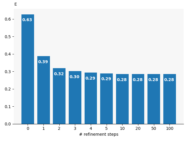
To investigate the impact of refinement on the downstream error estimate we used $20$ MNIST images, rotated each with $3$ random angles and then proceeded to calculate the inverse. In the calculation, we considered the range $\Gamma_{\pm}=10$ . We see that a low number of refinements have a large impact on the error but the returns become quickly diminishing. The impact on the run time of a single additional refinement step is negligible.

Appendix C Inverse for Rich Images

IndivSPT performs poorly on large images, such as those from ImageNet as the inverse computation outlined in Section 6 produces a too large over-approximation of ${\bm{x}}$ leading to $E$ estimates of around $40$ , while manageable value would be $\leq 2$ .

Fig. 5 shows the computed inverse for such images. We observe a pattern of artifacts in the inverse, where the pixel value can not be narrowed down sufficiently resulting in the large estimate of $E$ . The result of the refined inverse is perfectly recognizable to a human observer (or a neural network), highlighting the promise of the algorithm for future applications.

Appendix D Experiment Details

D.1 Details for Section 7.3

To evaluate BaseSPT we use the following classifiers. Note that Table 7 in Section E.1 contains results for further datasets:

MNIST [34]

We trained a convolutional network consisting of $\text{{Conv2d}}(k,n)$ , with $k\times k$ filter size, $n$ filter channels and stride 1, batch norm BN [35], maximum pooling MaxPool(k) on $k\times k$ grid, $\text{{Dropout}}(p)$ [36] with probability $p$ and linear layers $\text{{Lin}}(a,b)$ from $\mathbb{R}^{a}$ to $\mathbb{R}^{b}$ .

		$\displaystyle\text{{Conv2d}}(5,32),\text{{ReLU}},\text{{BN}}$
		$\displaystyle\text{{Conv2d}}(5,32),\text{{ReLU}},\text{{MaxPool}(2)},\text{{Dropout}}(0.2)$
		$\displaystyle\text{{Conv2d}}(3,64),\text{{ReLU}},\text{{BN}}$
		$\displaystyle\text{{Conv2d}}(3,64),\text{{ReLU}},\text{{BN}},\text{{MaxPool}(2)},\text{{Dropout}}(0.2)$
		$\displaystyle\text{{Conv2d}}(3,128),\text{{ReLU}},\text{{BN}}$
		$\displaystyle\text{{Conv2d}}(1,128),\text{{ReLU}},\text{{BN}},\text{{Flatten}}$
		$\displaystyle\text{{Lin}}(128,100),\text{{ReLU}}$
		$\displaystyle\text{{Lin}}(100,10)$

We used data normalization for MNIST and trained for 180 epochs with SGD, starting from learning rate $0.01$ , decreasing it by a factor of $10$ every $60$ epochs. No other pre-processing was used.

FashionMNIST [37]

We trained a ResNet-18 with data normalization. We trained for 180 epochs with SGD with an initial learning rate of $0.01$ , lowering it by a factor of 10 every $60$ epochs.

CIFAR [33]

We trained a ResNet-18 with data normalization. We trained for 90 epochs with SGD with an initial learning rate of $0.1$ , lowering it by a factor of 10 every $30$ epochs. We resized GTSRB images to $32\times 32\times 3$ .

ImageNet [31]

We used the pre-trained ResNet50 from torchvision: https://pytorch.org/docs/stable/torchvision/models.html.

D.2 Details for Section 7.4

In Section 7.4 we use a ResNet-18 architecture for MNIST and a ResNet-110 for CIFAR-10 and, as in, Section D.1, ResNet-50 for (R)ImageNet. We trained them to be robust to image transformations (rotation, translation) as well as $\ell^{2}$ noise.

To train networks that perform well when randomized smoothing is applied, we utilize the training procedure SmoothAdv_PGD as outlined in Salman et al. 2019a. For each batch of samples we apply a randomized data augmentation, vignetting, and Gaussian blur. After this prepossessing we then apply SmoothAdv_PGD (noise restricted to the vingetted area) then evaluate or train on the batch.

The intuition behind the Gaussian blur is that many artifacts, such as the interpolation error are have high frequencies. The blur acts as a low-pass filter and discards high frequency noise. This does not strongly impact the classification accuracy, but drastically reduces the error estimate and therefore the amount of noise that needs to be added for robust classification. The filter is parameterized by $\sigma_{b}$ and the filter size $s_{b}$ . Formally the filter is a convolution with a filter matrix $F\in\mathbb{R}^{s_{b}\times s_{b}}$ . Each entry in $F$ is filled with values of a two dimensional Gaussian distribution centered at the center of the matrix and evaluated at the center of the entry. Afterwards the matrix is normalized such that $\sum_{i,j},F_{i,j}=1$ .

In the error estimation and inference we use the same prepossessing as during training.

MNIST

For MNIST we use a ResNet-18 (that takes a single color channel in the input layer), which we trained with PGD step size $0.2$ , batch size $1024$ , and initial learning rate $0.01$ over 180 epochs, lowering the learning rate every 60 epochs. For DistSPT^D we use $\sigma=0.22$ and data augmentation with rotations in $[-90,90]$ degrees for the rotation model and $\sigma=0.3$ and random translations of $\pm 50\%$ for the translation model. For the Gaussian blur we use $\sigma_{b}=2.0$ with filter size $s_{b}=5$ on all models.

For DistSPT^x we use a model trained with $\sigma=0.15$ for rotations and but the same translation model.

CIFAR-10

For DistSPT^D we train a ResNet-110 with batch size 256, $\sigma=0.25$ and random rotations in $[-60,60]$ as well as SmoothAdv_PGD with $m=1$ samples, $t=8$ steps and warmup of 10 epochs for a perturbation size of $0.5$ . We train over 150 epochs and lower the learning rate every 50 steps. For the Gaussian blur we use $\sigma_{b}=1.0$ and $s_{b}=5$ .

For DistSPT^x we use $\sigma=0.12$ , perturbation size of $0.25$ , $m=8$ and $t=1$ and keep other parameters the same. Both variants take about 17 minutes per epoch on a single GeForce RTX 2080 Tis.

(Restricted) ImageNet

We trained with a batch size of 400 for 90 epochs using stochastic gradient decent with a learning rate starting at 0.1, which is decreased by a factor 10 every 30 epochs. On both datasets , we used $\sigma=0.5$ and PGD step size $1.0$ , as well as $\sigma_{b}=2.0$ and $s_{b}=5$ . For Restricted ImageNet we train with random rotation in $[-60,60]$ and for ImageNet in $[-30,30]$ .

Training 1 epoch of ImageNet with 6 GeForce RTX 2080 Tis and a 16-core node of aw Intel(R) Xeon(R) Gold 6242 CPU @ 2.80GHz takes roughly 2.5 hours and roughly 30 minutes for Restricted ImageNet. For the accuracy of $b$ in Table 3, we evaluate four settings — with vingetting, with Gaussian blur, with both and with neither — and report the highest. Table 5 shows a comparison across all settings.

Table 5: Base models evaluated on the whole data set either with Gaussian blur (G), Vingetting (V), both or neither.

Model	$T^{I}$	Standard	+G	+V	+G+V
MNIST, DistSPT^D	$R^{I}$	0.98	0.98	0.98	0.98
MNIST, DistSPT^x	$R^{I}$	0.98	0.98	0.98	0.98
MNIST	$\Delta^{I}$	0.94	0.92	0.94	0.93
CIFAR-10 DistSPT^D	$R^{I}$	0.34	0.36	0.56	0.56
CIFAR-10 DistSPT^x	$R^{I}$	0.75	0.76	0.70	0.70
RImageNet	$R^{I}$	0.77	0.77	0.78	0.77
ImageNet	$R^{I}$	0.38	0.32	0.38	0.32

To sample $E$ for (R)ImageNet we use a server with an AMD EPYC 7601 processor with 128 threads.

Table 6 shows a version Table 3 in the layout of the version of this paper published at NeurIPS’20.

Table 6: Evaluation of DistSPT for

T^{I}:=R^{I}

\epsilon_{\max}

is computed on the training set. We show the test set accuracy of

b

, certified accuracy of

g

and distribution of the obtained certification radius

r_{\gamma}

, along with the average run time

t

and the number of used samples

n_{\gamma},n_{\delta}

. ^# denotes values obtained by sampling. Each certificate hold with overall confidence

0.99

Dataset	$\epsilon_{\max}$	$E$	$b$	$g$	$25^{\text{th}}$	$50^{\text{th}}$	$75^{\text{th}}$	t [s]	$n_{\gamma}$	$n_{\delta}$
			Acc.		$r_{\gamma}$ percentile
MNIST	0.36	0.45	0.98	0.89	52.95	57.22	57.22	21.56	200	10000
CIFAR-10	0.51	0.55	0.56	0.31	24.80	$30.00^{\dagger}$	$30.00^{\dagger}$	89.75	50	15000
CIFAR-10	0.51	0.55	0.56	0.32	$30.00^{\dagger}$	$30.00^{\dagger}$	$30.00^{\dagger}$	351.47	200	15000
RImageNet	0.91	1.20	0.78	0.74	$30.00^{\dagger}$	$30.00^{\dagger}$	$30.00^{\dagger}$	100.73	50	2500
RImageNet	0.91	1.35	0.78	0.64	$30.00^{\dagger}$	$30.00^{\dagger}$	$30.00^{\dagger}$	100.13	50	2500
ImageNet	0.91	0.95	0.38	0.30	14.51	24.34	$30.00^{\dagger}$	100.21	50	2500
ImageNet	0.91	1.20	0.38	0.23	12.38	21.47	$30.00^{\dagger}$	100.73	50	2500
ImageNet	0.91	1.35	0.38	0.16	10.46	21.47	$30.00^{\dagger}$	100.44	50	2500

D.3 Details for Section 7.5

For rotation we use the $\sigma=0.22$ model as in Section D.2 and for translation also the same model.

Appendix E Additional Experiments

E.1 Additional Results for Section 7.3

Table 7: Extended version of Table 2. Evaluation of BaseSPT on 1000 images. The attacker used worst-of-100. We use

n_{\gamma}=1000,\sigma_{\gamma}=\Gamma_{\pm}

Dataset	$T^{I}$	$\Gamma_{\pm}$	$b$	$b$	$g$	t [s]
			Acc.	adv. Acc.
MNIST	$R^{I}$	$30^{\circ}$	0.99	0.73	0.99	0.97
FMNIST	$R^{I}$	$30^{\circ}$	0.91	0.13	0.87	7.98
CIFAR-10	$R^{I}$	$30^{\circ}$	0.91	0.26	0.85	0.95
GTSRB	$R^{I}$	$30^{\circ}$	0.91	0.30	0.88	8.00
ImageNet	$R^{I}$	$30^{\circ}$	0.76	0.56	0.76	5.43
MNIST	$\Delta^{I}$	$4$	0.99	0.03	0.53	0.86
FMNIST	$\Delta^{I}$	$4$	0.91	0.10	0.50	6.12
CIFAR-10	$\Delta^{I}$	$4$	0.91	0.44	0.79	0.95
GTSRB	$\Delta^{I}$	$4$	0.91	0.30	0.63	5.17
ImageNet	$\Delta^{I}$	$20$	0.76	0.65	0.75	6.70

Table 7 is an extended version of Table 2 and provides results for additional datasets.

Table 8: We first use BaseSPT to obtain the certification radius

r_{\gamma}

on 30 images and subsequently sample from the parameter space indicated by

\Gamma_{\pm}=r_{\gamma}

and checked whether the certificate holds for them. We use 30 samples and

n_{\gamma}=2000

samples for the smoothed classifier. The last column shows the number of images for which we found violations.

Dataset	$T^{I}$	$\Gamma_{\pm}$	median $r_{\gamma}$	$r_{\gamma}$ violated
MNIST	$R^{I}$	$30^{\circ}$	28.34	0
FMNIST	$R^{I}$	$30^{\circ}$	13.45	1
CIFAR-10	$R^{I}$	$30^{\circ}$	19.16	14
GTSRB	$R^{I}$	$30^{\circ}$	20.93	0
ImageNet	$R^{I}$	$10^{\circ}$	27.13	1
MNIST	$\Delta^{I}$	$4$	1.12	0
FMNIST	$\Delta^{I}$	$4$	1.78	1
CIFAR-10	$\Delta^{I}$	$4$	4.76	14
GTSRB	$\Delta^{I}$	$4$	2.58	0
ImageNet	$\Delta^{I}$	$20$	16.43	0

Table 9: Same setup as in Table 8, but with circular vignetting.

Dataset	$T^{I}$	$\Gamma_{\pm}$	median $r_{\gamma}$	$r_{\gamma}$ violated
MNIST	$R^{I}$	$30^{\circ}$	28.34	0
FMNIST	$R^{I}$	$30^{\circ}$	17.07	0
CIFAR-10	$R^{I}$	$30^{\circ}$	11.49	10
GTSRB	$R^{I}$	$30^{\circ}$	25.28	0

E.2 “Certification Radius” of BaseSPT

As BaseSPT uses Theorem 3.2 to justify the heuristic, this also makes it tempting to use the bound $r_{\gamma}$ provided by it. However, as the assumptions of Theorem 3.2 are violated it does not formally present a certification radius. Here we investigate if and how much it holds nevertheless. To do this we construct a smoothed classifier $g$ from an undefended base classifier $b$ and calculated the certification radius $r_{\gamma}$ . Subsequently, we sampled 100 new rotated images in the parameter space induced by $\Gamma_{\pm}=r_{\gamma}$ and evaluated on them. The results are shown in Table 8. While generally robust, the radius does not constitute a certificate, as we can clearly find violations.

In the context of rotation $R^{I}$ we add circular vignetting (as we do for DistSPT and IndivSPT) to make the behavior closer to a composing transformation. For this experiment, we retrained the same networks, but applied the vignette during training. Results are shown in Table 9 where we can see that this already decreases the number of violations for CIFAR-10 and FMNIST. In a final step we assume knowledge of the attacker parameter $\gamma$ and replace $R^{I}_{\beta}\circ R^{I}_{\gamma}$ (for the same images) with $R^{I}_{\beta+\gamma}$ in the evaluation of the classifier, in which case Theorem 3.2 should hold and indeed we don’t observe any more violations.

E.3 Additional Results for Section 7.4

Beyond Bilinear Interpolation

BaseSPT and DistSPT can directly be applied to image transformations using other interpolation schemes without any adaption. IndivSPT, however, requires the adaption of the inverse algorithm. While this is generally possible, we consider it beyond the scope of this work.

We guess (based on $1000$ samples) and verify $E$ using $1000$ samples for ${\bm{x}}$ and $8000$ for $\beta$ . We summarize these results in Table 10. On datasets other than MNIST we observe $E$ larger than possible. At manageable levels, the $q_{E}$ becomes too low for practical purposes.

On MNIST with the same settings as for DistSPT^D we certify 90 out of 100 images at $r_{\gamma}=30$ (for bilinear interploation with $E=0.45$ 91 can be certified).

Table 10:

E

and

q_{E}

for bicubic interpolation.

Dataset	$E$	$q_{E}$
MNIST	0.5	0.99
CIFAR-10	1.10	0.99
CIFAR-10	0.55	0.27
ImageNet	2.50	0.99
ImageNet	1.20	0.28

E.4 Audio Volume Change

To show that our method can be used beyond image transformation we showcase an adaption to audio volume changes. The volume of an audio signal can be changed by multiplying the signal with a constant. In order to change the signal ${\bm{x}}$ by $\beta$ (measured in decibel $[\beta]=\text{dB}$ ) we multiply ${\bm{x}}$ by $10^{\beta/20}$ . Thus the transformation is $\psi_{\beta}({\bm{x}}):=10^{\beta/20}\cdot{\bm{x}}$ , which composes:

\psi_{\beta}\circ\psi_{\gamma}({\bm{x}})=10^{(\beta+\gamma)/20}\cdot{\bm{x}}=\psi_{\beta+\gamma}({\bm{x}}).

In practice such signals are stored in final precision, e.g. 16-bit, thus potentially introducing rounding errors, with an $\ell^{2}$ -norm bound by $E$ . If this is ignored BaseSPT can be applied to obtain guarantees. Otherwise, DistSPT and IndivSPT can be used to obtain sound bounds.

To evaluate this we use the speech commands dataset [38], consisting of 30 different commands, spoken by people, which are to be classified. The length of the recordings are one second each. We use a classification pipeline that converts audio wave forms into MFCC spectra [39] and then treats these as images and applies normal image classification. We use a ResNet-50, that was trained with Gaussian noise, but not SmoothAdv_PGD. We apply the noise before the waveform is converted to the MFCC spectrum.

For DistSPT we estimate $E$ to be $0.005$ with the parameters $\rho_{E}=0.05,\sigma_{\gamma}=3$ and $\Gamma=3$ (for which $q_{E}\approx 0.75$ ). On 100 samples, the base classifier $f$ was correct $93$ times. At $r_{gamma}$ of 1, 2, 3 and 4 the certified accuracy was 0.92, 0.89, 0.83 and 0.69 respectively. This corresponds to $\pm 1.12$ , $\pm 1.26$ , $\pm 1.41$ and $\pm 1.58$ dB. At $n_{\gamma}=150$ and $n_{\epsilon}=400$ the average certification time was $26.80$ s. We use $\alpha_{\gamma}=0.004,\alpha_{\epsilon}=\tfrac{0.005}{n_{\gamma}}$ , assuming (but not computing) $\alpha_{E}=0.001$ here, for a total confidence of $0.99$ in each certificate.

To investigate IndivSPT we use $\sigma_{\gamma}=0.85,\Gamma=1.05$ . For 92 out of $100$ perturbed audio signals to compute $\epsilon$ . We obtained $\epsilon_{\max}\leq 0.0055$ and for 68 an $\epsilon\leq 0.005$ , which together with our results for DistSPT suggests the applicability of the method. For each signal we used $100$ samples for $\beta$ . For cases with $\epsilon_{\max}>0.0055$ we in fact observed $\epsilon_{\max}\gg 0.0055$ , as here many parts of the signal were amplified beyond the precision of the 16-bit representation and clipped to $\pm 1$ . This makes the information unrecoverable and sound error bound estimates large.

Table 11: Maximum observed errors and without gaussian blur (G) and without vignetting (V).

Dataset	Both	-V	-G	-V-G
MNIST	0.36	0.36	2.47	2.51
CIFAR-10	0.51	6.08	2.66	18.17
ImageNet	0.91	70.66	9.25	75.69

Table 12: Correct classifications and by the model and verifications by DeepG [11], with and without vignetting (V), out of 100 images.

Model	Correct	[11]	[11]+V
MNIST	98	86	87
CIFAR-10	74	65	32
CIFAR-10+V	78	63	23

Appendix F Further Comparison and Ablation

To show that the vignette and Gaussian blur are essential to our algorithm we perform a small ablation study. Table 12 shows the maximal error observed when sampling as in DistSPT. We use the same setup as in Section 7.4, but with 10000 samples for ImageNet.

Both, vignetting and Gaussian blur reduce the error bound significantly for DistSPT and IndivSPT. On CIFAR-10 and ImageNet vignetting is very impactful because the corners of images are rarely black in contrast to MNIST. Li et al. 2020 uses vignetting for the same reason. Without either of the methods bounding the error would not be feasible.

For IndivSPT vignetting is crucial, even for MNIST, as we can make no assumptions for parts that are rotated into the image. Thus we need to set these pixels to the full $[0,1]$ interval (see Fig. 2). Without Gaussian blur the certification rate drops to $0.11$ .

Further, we extend this comparison to related work: We extended Balunovic et al. 2019 (Table 1 in their paper) to include vignetting. The results are shown in Table 12. We also retrained their CIFAR-10 model with vignetting (CIFAR-10+V) for completeness. While vignetting on MNIST slightly helps (+1 image verified) on CIFAR-10 it leads to a significant drop. Including Gaussian blur into [11] would require non-trivial adaption of the method. However, we implemented this for interval analysis (on which their method is built) and found no impact on results.

Certified Defense to Image Transformations via Randomized Smoothing

Abstract

1 Introduction

Certification guarantees

Guarantees with ℓp\ell^{p} norms

Key challenge: guarantees for geometric perturbations

This work: certification beyond ℓp\ell^{p} norms

BaseSPT

IndivSPT

DistSPT

2 Related Work

ℓp\ell^{p} norm based certification and defenses

Semantic perturbations

3 Generalization of Smoothing

Theorem 3.1 (From [7]).

Theorem 3.2.

4 Certification with interpolation and rounding errors

Obtaining probabilistic guarantees from Theorem 3.2

5 Calculation of error bounds

5.1 Distributional bounds for DistSPT

5.2 Individual bounds for IndivSPT

6 Inverse Computation

Transformations

Bilinear interpolation

Step 1

Step 2

Step 3

Refined Inverse

6.1 Example

Step 1

Step 2

Step 3

7 Experimental Evaluation

7.1 Instantiation in Practice

7.2 Setup

7.3 BaseSPT

DistSPTD

DistSPTx

Comparison to other work

7.5 IndivSPT Footnote 1

7.6 Limitations & Generalization

8 Conclusion

9 Broader Impact

Acknowledgments and Disclosure of Funding

References

Appendix A Proof of Theorem 3.2

Theorem A.1.

Proof.

Lemma 1.

Proof.

Lemma 2.

Proof.

Theorem (Theorem 3.2 restated).

Appendix B Inverse and Refinement

B.1 Details for Step 2

B.2 Algorithm

B.3 Experimental Evaluation

Appendix C Inverse for Rich Images

Appendix D Experiment Details

D.1 Details for Section 7.3

D.2 Details for Section 7.4

MNIST

CIFAR-10

(Restricted) ImageNet

D.3 Details for Section 7.5

Appendix E Additional Experiments

E.1 Additional Results for Section 7.3

E.2 “Certification Radius” of BaseSPT

E.3 Additional Results for Section 7.4

Beyond Bilinear Interpolation

E.4 Audio Volume Change

Appendix F Further Comparison and Ablation

Guarantees with $\ell^{p}$ norms

This work: certification beyond $\ell^{p}$ norms

$\ell^{p}$ norm based certification and defenses

DistSPT^D

DistSPT^x