Supervised Enhanced Soft Subspace Clustering (SESSC) for TSK Fuzzy Classifiers

Let the training dataset be $\mathcal{D}=\{\bm{x}_{n},\bm{y}_{n}\}_{n=1}^{N}$, in which $\bm{x}_{n}=[x_{n,1},...,x_{n,D}]^{T}$ is a $D$-dimensional input vector, and $\bm{y}_{n}=[y_{n,1},...,y_{n,C}]$ the corresponding $C$-class one-hot encoding label vector. $X\in\mathbb{R}^{N\times D}$ is the input matrix containing all inputs, and $Y\in\mathbb{R}^{N\times C}$ the corresponding label matrix.

Suppose the TSK fuzzy classifier has $R$ rules, in the following form:

where $\tilde{X}_{r,d}$ ($r=1,...,R$; $d=1,...,D$) is a Gaussian membership function (MF) for the $d$-th antecedent in the $r$-th rule, and $b_{r,d}^{c}$ ($c=1,...,C$) are the consequent parameters for the $c$-th class.

Let $V_{r,d}$ be the center of the Gaussian MF $\tilde{X}_{r,d}$, and $\Sigma_{r,d}$ be the corresponding standard deviation. Then, the membership grade of $x_{n,d}$ on $\tilde{X}_{r,d}$ is:

and its firing level on the $r$-th rule is

The normalized firing level is:

and the estimate for the $c$-th class, $\hat{y}^{c}(\bm{x}_{n})$, is

Once the antecedent parameters are initialized, LSE can be used to estimate the consequent parameters.

For a zero-order TSK fuzzy classifier, i.e., $b_{r,0}^{c}$ is adjustable whereas $b_{r,d}^{c}=0$ ($r=1,...,R;d=1,...,D;c=1,...,C$), we can define

Then, the one-hot coding matrix $Y$ is estimated by

and the optimal $B$ can be solved by LSE, i.e.,

where $\lambda$ is the weight of $L_{2}$ regularization in LSE.

For first-order TSK fuzzy classifier, we can define

Then, the optimal $B$ is still solved by (10).

FCM [9] can be used to initialize the antecedent part of the $R$ rules of a multi-class TSK fuzzy classifier:

where $U_{n,r}$ is the membership grade of $\bm{x}_{n}$ in the $r$-th cluster, $\bm{v}_{r}$ (the $r$-th row of $V$) the center of the $r$-th cluster, and $m$ the fuzzy index.

Once $U$ and $V$ are obtained, the standard deviation of $\tilde{X}_{r,d}$ can be estimated by:

where $h$ is an adjustable scaling parameter.

When the data dimensionality is high, the pairwise distances $\|\bm{x}_{n}-\bm{v}_{r}\|^{2}_{2}$ in (18) become similar for different $n$ and $r$. As a result, the cluster centers obtained by the original FCM converge to the center of the input data space [18], losing their discriminability. To remedy this problem, SSC uses weighted Euclidean distances, i.e.,

where $\bm{w}_{r}\in\mathbb{R}^{1\times D}$ is a weight vector associated with $\bm{v}_{r}$.

The cost function of AWFCM [26], using weighted Euclidean distances, is:

where $W=[\bm{w}_{1};\ldots;\bm{w}_{R}]\in\mathbb{R}^{R\times D}$.

The cost function of SCAD [27], which further adds an exponential term $t$ to the weights, is:

Zhou et al. [28] proposed EWFCM, which uses entropy as a regularization term to control the weights, and modifies the cost function of FCM to:

where $\gamma$ is a user-specified regularization parameter.

In addition to the within-cluster compactness, the between-cluster separation is also very important in clustering [30]. ESSC [19] takes the between-cluster separation into consideration, and its cost function is

where $\bm{v}_{0}=\frac{1}{N}\sum_{n=1}^{N}\bm{x}_{n}$ is the center of all data samples, and $\eta\in[0,1)$ is a user-specified regularization parameter.

Although SSC can be used to learn a better cluster structure than the traditional FCM, it does not utilize the label information in supervised learning. Ideally, a cluster should only contain data samples with the same label. Recently, supervised fuzzy partition (SFP) [31] was proposed to tackle this problem. Its objective function integrates SSC and label information:

where $\bm{z}_{r}\in\mathbb{R}^{1\times C}$ indicates the label prediction for Cluster $r$, and $\ell$ a loss function.

In addition to the utilization of label information, SFP uses the entropy, instead of the fuzzy index $m$, to regularize the membership grades $U$. However, it does not consider the between-cluster separation, compared with ESSC.

We propose SESSC to integrate the label information with ESSC, which uses the following cost function to constrain the labels in each cluster, following [31]:

where $Z_{r,c}$ indicates the probability that Cluster $r$ belongs to Class $c$. Clearly, $\sum_{c=1}^{C}Z_{r,c}=1$, $r=1,...,R$.

An equivalence of (26) is:

where $\bm{z}_{r}=[Z_{r,1},...,Z_{r,C}]$. (27) can be easily extended to regression problems.

Minimizing (26) or (27) leads to the optimal label $Z_{r,c}$:

where

Adding (26) to the cost function of ESSC, we obtain the cost function for our proposed SESSC:

(30) can be solved using the Lagrange multiplier method. We first form the following Lagrangian function:

where $\bm{\alpha}=[\alpha_{1},...,\alpha_{N}]$ and $\bm{\zeta}=[\zeta_{1},...,\zeta_{R}]$ are Lagrangian multiplier coefficients.

When $V$, $W$ and $Z$ are fixed, we can compute the optimal value of $U$ by setting $\partial J/\partial U_{n,r}=0$ and $\partial J/\partial\alpha_{n}=0$, i.e.,

which lead to

where

When $U$, $W$ and $Z$ are fixed, we can compute the optimal value of $V$ by setting $\partial J/\partial V_{r,d}=0$, i.e.,

which leads to

When $U$, $V$ and $Z$ are fixed, we can compute the optimal value of $W$ by setting $\partial J/\partial W_{r,d}=0$ and $\partial J/\partial\zeta_{r}=0$, i.e.,

which lead to

where

When $U$, $V$ and $W$ are fixed, the label of the $r$-th cluster, $\bm{z}_{r}$, can be computed by (28).

The pseudo-code of SESSC is summarized in Algorithm 1. The center matrix $V$ is initialized from $k$-means clustering.

A toy example illustrating a four-class classification problem and the corresponding cluster centers obtained from ESSC and SESSC are shown in Fig. 1. The data samples were generated from a 2-dimensional Gaussian distribution $\bm{N}(0,1)$, and each quadrant represents a different class. Clearly, the cluster centers generated from SESSC are more reasonable, and hence may lead to better classification performance when used to initialize a TSK fuzzy classifier.

SESSC itself can be used as a classifier. Following the approach used in [31], for a test sample $\bm{x}_{t}$, we can estimate the memberships by:

where

Then, the label matrix $\hat{Y}$ is computed as

where

SESSC can also be used to initialize the antecedent part of a TSK fuzzy classifier, and then LSE can be used to estimate the consequent parameters. This approach is denoted SESSC-LSE in this paper. Its pseudo-code is given in Algorithm 2.

First, we evaluated the performances of our proposed SESSC and SESSC-LSE on two synthetic 2-dimensional datasets, concentric circles and spiral. The parameters of SESSC were $R=\{5,10,15,20\}$, $\gamma=100$, $\eta=0.01$ and $\beta=0.1$. Zero-order SESSC-LSE was used here for a fair comparison. Additional parameters for SESSC-LSE were $h=1$ and $\lambda=0.01$. The results are shown in Fig. 2, in which the dots represent the generated data samples, and the black curves the decision boundaries learned by SESSC and SESSC-LSE.

Fig. 2 shows that:

1. 1.

   When $R$, the number of clusters, increased, the SESSC decision boundaries became smoother and closer to the true decision boundaries. This demonstrated that our proposed SESSC can fit smooth decision boundaries and achieve good generalization performance.

2. 2.

   For the same $R$, SESSC-LSE outperformed SESSC, which indicated that SESSC-LSE can further improve the classification performance.

Next, we evaluated our proposed algorithms on nine classification datasets from the UCI Machine Learning Respository¹¹ 1 http://archive.ics.uci.edu/ml/index.php. Their characteristics are summarized in Table II. For each dataset, we randomly selected 70% samples as the training set and the remaining 30% as the test set 30 times to get 30 different data splits. We ran each algorithm on these 30 data splits and report the average performance.

Some datasets contain both numerical and categorical features. The categorical features were converted to numerical ones by one-hot encoding. Then, all features were normalized by $z$-score using mean and standard deviation computed from the training set.

Since some datasets have significant class imbalance, both raw classification accuracy (RCA) and balanced classification accuracy (BCA) were used as the performance measure:

• •

  RCA: The total number of correct classifications divided by the total number of samples.

• •

  BCA: The average of per-class RCAs, which is less affected by class imbalance.

We used LSE to compute the consequent parameters for all TSK fuzzy classifiers [see (10)]. We replaced SESSC in SESSC-LSE by three different clustering algorithms (FCM, EWFCM, and ESSC) to compare their performances with SFP and the proposed SESSC and SESSC-LSE. Because SFP and SESSC are zero-order fuzzy classifiers, we did not compare them with first-order fuzzy classifier (FCM-LSE, EWFCM-LSE, ESSC-LSE and SESSC-LSE).

The values or search ranges of the parameters in different algorithms are shown in Table III. We set $R=30$ to keep the fuzzy classifiers concise so they can have interpretability. Note that in the original SFP paper [31], the number of clusters $R$ was optimized in $[D,N]$, which was much larger than 30 used in our experiments. This might be the reason why SFP performed worse than other SSC based fuzzy classifiers. In the actual implementation [31], SFP used modified parameters $\gamma^{\prime}$, $\alpha^{\prime}$, $\lambda^{\prime}$ during grid research, where $\gamma=(1-\gamma^{\prime})/\gamma^{\prime}$, $\alpha=(1-\alpha^{\prime})/\alpha^{\prime}$ and $\lambda=(1-\lambda^{\prime})/\lambda^{\prime}$.

We tuned all parameters using 5-fold cross validation on the training set and chose the combination with the highest average BCA. The best $\gamma$, $\eta$ and $\beta$ from SESSC were used in SESSC-LSE.

The average test RCAs and BCAs of zero-order fuzzy classifiers are shown in Table IV. The best performance on each dataset is marked in bold. The ranks of the average RCAs and BCAs are shown in Table V.

Tables IV andV show that:

1. 1.

   For zero-order fuzzy classifiers, our proposed SESSC-LSE achieved the best RCA on six out of the nine datasets, and best BCA on eight out of the nine datasets. SESSC-LSE’s performance was also close to the best on the remaining datasets. On average, SESSC-LSE achieved the best RCA and BCA, and also ranked the first.

2. 2.

   Our proposed SESSC and SESSC-LSE performed better on datasets with class imbalance. For instance, FCM-LSE and EWFCM-LSE achieved much higher RCAs on WPBC, but their BCAs were almost random (50% BCA for binary classification). Although SESSC had a lower average RCA than EWFCM-LSE and ESSC-LSE, its average BCA was higher. The proposed SESSC-LSE further improved the BCA performance of SESSC.

3. 3.

   On average, all four SSC-based algorithms (EWFCM-LSE, ESSC-LSE, SFP and SESSC-LSE) outperformed FCM-LSE. This demonstrated that SSC-based clustering algorithms can result in clusters with higher discriminability on high-dimensional datasets.

We also compared four first-order TSK classifiers and show their performances in Tables VI and VII. All four of them performed similarly, and all three SSC-based classifiers had stable performances (first-order FCM-LSE performed significantly worse than SSC-based classifiers on the Satellite dataset). This suggests that when the consequent complexity of the TSK fuzzy classifier increases, the antecedent initialization may become less important.

To further evaluate if the performance improvements of our proposed SESSC-LSE over others were statistically significant, we also performed non-parametric multiple comparison tests on the RCAs and BCAs using Dunn’s procedure [32], with a $p$-value correction using the False Discovery Rate method [33]. The results are shown in Tables VIII and IX respectively for zero-order and first-order TSK classifiers, where the statistically significant ones are marked in bold.

Table VIII shows that our proposed zero-order SESSC-LSE significantly outperformed all other approaches. In addition, all SSC-based clustering algorithms, except SFP, significantly outperformed FCM-LSE, indicating that the SSC-based clustering algorithms are more suitable for initializing TSK fuzzy classifiers on high-dimensional datasets.

Table IX shows that different clustering approaches do not affect the performance of first-order TSK fuzzy classifiers significantly.

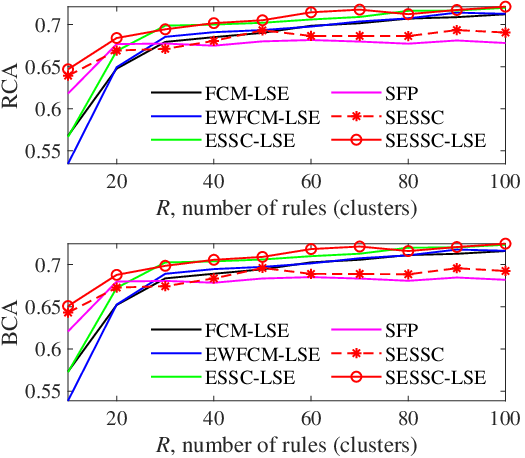
Since the performance of a TSK fuzzy classifier varies with $R$, the number of rules, we changed $R$ in the six zero-order algorithms from 10 to 100, while keeping all other parameters at their optimal values ($\gamma=10$, $\eta=0.1$, $\beta=1$, $\alpha=0.01$ and $h=100$ for SESSC and other TSK fuzzy classifiers; $\gamma^{\prime}=0.9$, $\alpha^{\prime}=0.45$ and $\lambda^{\prime}=0.05$ for SFP) on the Vehicle dataset to study the performances of the five algorithms. The results are shown in Fig. 3. On average, SESSC-LSE always performed the best. SESSC and SESSC-LSE performed much better than other unsupervised clustering algorithms when $R$ was small.

We analyzed the convergence of our proposed SESSC algorithm on the Vehicle dataset with different number of clusters. The median value of the cost function from different runs are shown in Fig. 4. SESSC converged quickly after a small number of iterations, e.g., four, which is desirable in practice.

The proposed SESSC algorithm has four parameters, $R$, $\gamma$, $\eta$ and $\beta$. We also tested how they affected the classification performance on three datasets (Vehicle, Biodeg and DRD), by fixing three of them at their default values ($R=30$, $\gamma=10$, $\eta=0.1$ and $\beta=1$) and varying the remaining one. The results are shown in Fig. 5. Generally, the performance is stable over a wide parameter range, which is desirable.

References

- [1] A.-T. Nguyen, T. Taniguchi, L. Eciolaza, V. Campos, R. Palhares, and M. Sugeno, “Fuzzy control systems: Past, present and future,” IEEE Computational Intelligence Magazine, vol. 14, no. 1, pp. 56–68, 2019.
- [2] P.-C. Chang and C.-H. Liu, “A TSK type fuzzy rule based system for stock price prediction,” Expert Systems with Applications, vol. 34, no. 1, pp. 135–144, 2008.
- [3] R.-J. Wai and P.-C. Chen, “Intelligent tracking control for robot manipulator including actuator dynamics via TSK-type fuzzy neural network,” IEEE Trans. on Fuzzy Systems, vol. 12, no. 4, pp. 552–560, 2004.
- [4] Y. Jiang, D. Wu, Z. Deng, P. Qian, J. Wang, G. Wang, F.-L. Chung, K.-S. Choi, and S. Wang, “Seizure classification from EEG signals using transfer learning, semi-supervised learning and TSK fuzzy system,” IEEE Trans. on Neural Systems and Rehabilitation Engineering, vol. 25, no. 12, pp. 2270–2284, 2017.
- [5] L. A. Zadeh, “Toward a generalized theory of uncertainty (GTU)—-an outline,” Information Sciences, vol. 172, no. 1-2, pp. 1–40, 2005.
- [6] B. Rezaee and M. H. F. Zarandi, “Data-driven fuzzy modeling for Takagi–Sugeno–Kang fuzzy system,” Information Sciences, vol. 180, no. 2, pp. 241–255, 2010.
- [7] D. Wu, Y. Yuan, J. Huang, and Y. Tan, “Optimize TSK fuzzy systems for regression problems: Mini-batch gradient descent with regularization, DropRule and AdaBound (MBGD-RDA),” IEEE Trans. on Fuzzy Systems, 2020, in press.
- [8] Y. Cui and D. Wu, “Optimize TSK fuzzy systems for classification problems: Mini-batch gradient descent with uniform regularization and batch normalization,” IEEE Trans. on Fuzzy Systems, 2020, in press.
- [9] J. C. Bezdek, R. Ehrlich, and W. Full, “FCM: The fuzzy c-means clustering algorithm,” Computers & Geosciences, vol. 10, no. 2-3, pp. 191–203, 1984.
- [10] J. S. R. Jang, “ANFIS: Adaptive-network-based fuzzy inference system,” IEEE Trans. on Systems, Man, and Cybernetics, vol. 23, no. 3, pp. 665–685, 1993.
- [11] A. Priyono, M. Ridwan, A. J. Alias, R. A. O. K. Rahmat, A. Hassan, and M. A. M. Ali, “Generation of fuzzy rules with subtractive clustering,” Jurnal Teknologi, vol. 43, no. 1, pp. 143–153, 2005.
- [12] Z. Deng, K.-S. Choi, F.-L. Chung, and S. Wang, “Scalable TSK fuzzy modeling for very large datasets using minimal-enclosing-ball approximation,” IEEE Trans. on Fuzzy Systems, vol. 19, no. 2, pp. 210–226, 2010.
- [13] Z. Deng, L. Cao, Y. Jiang, and S. Wang, “Minimax probability TSK fuzzy system classifier: A more transparent and highly interpretable classification model,” IEEE Trans. on Fuzzy Systems, vol. 23, no. 4, pp. 813–826, 2014.
- [14] C.-T. Lin, C.-M. Yeh, S.-F. Liang, J.-F. Chung, and N. Kumar, “Support-vector-based fuzzy neural network for pattern classification,” IEEE Trans. on Fuzzy Systems, vol. 14, no. 1, pp. 31–41, 2006.
- [15] Y. Shi, R. Eberhart, and Y. Chen, “Implementation of evolutionary fuzzy systems,” IEEE Trans. on Fuzzy Systems, vol. 7, no. 2, pp. 109–119, 1999.
- [16] M. J. Gacto, M. Galende, R. Alcalá, and F. Herrera, “METSK-HDe: A multiobjective evolutionary algorithm to learn accurate TSK-fuzzy systems in high-dimensional and large-scale regression problems,” Information Sciences, vol. 276, pp. 63–79, 2014.
- [17] D. Wu and X. Tan, “Multitasking genetic algorithm (MTGA) for fuzzy system optimization,” IEEE Trans. on Fuzzy System, 2020, in press.
- [18] R. Winkler, F. Klawonn, and R. Kruse, “Fuzzy c-means in high dimensional spaces,” Int’l Journal of Fuzzy System Applications, vol. 1, no. 1, pp. 1–16, 2011.
- [19] Z. Deng, K.-S. Choi, F.-L. Chung, and S. Wang, “Enhanced soft subspace clustering integrating within-cluster and between-cluster information,” Pattern Recognition, vol. 43, no. 3, pp. 767–781, 2010.
- [20] L. Parsons, E. Haque, and H. Liu, “Subspace clustering for high dimensional data: A review,” ACM SIGKDD Explorations Newsletter, vol. 6, no. 1, pp. 90–105, 2004.
- [21] K. Sim, V. Gopalkrishnan, A. Zimek, and G. Cong, “A survey on enhanced subspace clustering,” Data Mining and Knowledge Discovery, vol. 26, no. 2, pp. 332–397, 2013.
- [22] C.-H. Cheng, A. W. Fu, and Y. Zhang, “Entropy-based subspace clustering for mining numerical data,” in Proc. of the ACM SIGKDD Int’l Conf. on Knowledge Discovery and Data Mining, San Diego, CA, Aug. 1999, pp. 84–93.
- [23] S. Goil, H. Nagesh, and A. Choudhary, “MAFIA: Efficient and scalable subspace clustering for very large data sets,” in Proc. of the ACM SIGKDD Int’l Conf. on Knowledge Discovery and Data Mining, vol. 443, San Diego, CA, Aug. 1999, p. 452.
- [24] C. C. Aggarwal and P. S. Yu, “Finding generalized projected clusters in high dimensional spaces,” in Proc. of the ACM SIGMOD Int’l Conf. on Management of Data, Dallas, TX, May 2000, pp. 70–81.
- [25] Z. Deng, K.-S. Choi, Y. Jiang, J. Wang, and S. Wang, “A survey on soft subspace clustering,” Information Sciences, vol. 348, pp. 84–106, 2016.
- [26] A. Keller and F. Klawonn, “Fuzzy clustering with weighting of data variables,” Int’l Journal of Uncertainty, Fuzziness and Knowledge-Based Systems, vol. 8, no. 06, pp. 735–746, 2000.
- [27] H. Frigui and O. Nasraoui, “Unsupervised learning of prototypes and attribute weights,” Pattern Recognition, vol. 37, no. 3, pp. 567–581, 2004.
- [28] J. Zhou, L. Chen, C. L. P. Chen, Y. Zhang, and H.-X. Li, “Fuzzy clustering with the entropy of attribute weights,” Neurocomputing, vol. 198, pp. 125–134, 2016.
- [29] P. Xu, Z. Deng, C. Cui, T. Zhang, K.-S. Choi, G. Suhang, J. Wang, and S. Wang, “Concise fuzzy system modeling integrating soft subspace clustering and sparse learning,” IEEE Trans. on Fuzzy Systems, vol. 27, no. 11, pp. 2176–2189, 2019.
- [30] K.-L. Wu, J. Yu, and M.-S. Yang, “A novel fuzzy clustering algorithm based on a fuzzy scatter matrix with optimality tests,” Pattern Recognition Letters, vol. 26, no. 5, pp. 639–652, 2005.
- [31] P. Ashtari, F. N. Haredasht, and H. Beigy, “Supervised fuzzy partitioning,” Pattern Recognition, vol. 97, p. 107013, 2020.
- [32] O. J. Dunn, “Multiple comparisons using rank sums,” Technometrics, vol. 6, no. 3, pp. 241–252, 1964.
- [33] Y. Benjamini and Y. Hochberg, “Controlling the false discovery rate: A practical and powerful approach to multiple testing,” Journal of the Royal Statistical Society: Series B, vol. 57, no. 1, pp. 289–300, 1995.