跳到论文正文
W Papers独立论文阅读器 arXiv:2002.12390 论文正文 计算阅读时间 · 0%
引用这篇论文根据当前论文元数据生成,正式投稿前建议核对。


License: arXiv.org perpetual non-exclusive license
arXiv:2002.12390v2 [hep-th] 08 Jul 2020

A Generalized Nachtmann Theorem in CFT

Sandipan Kundu

Department of Physics and Astronomy,
Johns Hopkins University, Baltimore, Maryland, USA

kundu@jhu.edu

Correlators of unitary quantum field theories in Lorentzian signature obey certain analyticity and positivity properties. For interacting unitary CFTs in more than two dimensions, we show that these properties impose general constraints on families of minimal twist operators that appear in the OPEs of primary operators. In particular, we rederive and extend the convexity theorem which states that for the family of minimal twist operators with even spins appearing in the reflection-symmetric OPE of any scalar primary, twist must be a monotonically increasing convex function of the spin. Our argument is completely non-perturbative and it also applies to the OPE of nonidentical scalar primaries in unitary CFTs, constraining the twist of spinning operators appearing in the OPE. Finally, we argue that the same methods also impose constraints on the Regge behavior of certain CFT correlators.

1 Introduction

The operator product expansion (OPE), as introduced in [1, 2, 3], provides an algebraic structure in quantum field theory (QFT) which is of fundamental importance. The OPE is particularly useful in conformal field theory (CFT) where it enjoys several nice properties. For example, two nearby scalar primary operators in any unitary CFT can be replaced by their OPE

𝒪1(x)𝒪2(y)=∑pc𝒪1​𝒪2​𝒪pDpμ1μ2⋯(x−y,∂y)𝒪μ1μ2⋯p(y),{\cal O}_{1}(x){\cal O}_{2}(y)=\sum_{p}c_{{\cal O}_{1}{\cal O}_{2}{\cal O}_{p}}D^{\mu_{1}\mu_{2}\cdots}_{p}\left(x-y,\partial_{y}\right){\cal O}_{\mu_{1}\mu_{2}\cdots}^{p}(y)\ , (1.1)

where the sum is over primary operators which transform homogeneously under the conformal group. The coefficient function Dμ1μ2⋯pD^{\mu_{1}\mu_{2}\cdots}_{p} is completely fixed by conformal symmetry up to an overall real coefficient c𝒪1​𝒪2​𝒪pc_{{\cal O}_{1}{\cal O}_{2}{\cal O}_{p}} which is commonly known as the OPE coefficient. Clearly, the operators 𝒪μ1μ2⋯p{\cal O}_{\mu_{1}\mu_{2}\cdots}^{p} that appear in the above OPE are also symmetric traceless representations of the Lorentz group and hence they can be labeled by scaling dimensions Δp\Delta_{p} and spins ℓp\ell_{p}. A key feature of the conformal OPE is that after insertion into any correlator, the OPE (1.1) converges absolutely even for finite separation x−yx-y [4, 5]. This fact plays a central role, both conceptually as well as technically, in the study of CFTs.

A CFT can be completely and uniquely defined by its OPEs. So, it is of interest to address the question of when a set of conformal OPEs defines a unitary and causal theory. In this paper, we answer a version of this question for interacting unitary CFTs in d>2d>2 dimensions by constraining the family of minimal twist operators that appears in the OPE (1.1), independent of the rest of the theory. The family of minimal twist operators is defined in the following way. First, consider all spin ℓ\ell primary operators that appear in the OPE (1.1). Among these operators, we pick the operator 𝒪~ℓ\tilde{{\cal O}}_{\ell} which has the lowest twist.11 1 The twist is defined in the usual way τ=Δ−ℓ\tau=\Delta-\ell. We define the set of operators {𝒪~ℓ|ℓ∈ℤ≥}\{\tilde{{\cal O}}_{\ell}\ |\ \ell\in{\mathbb{Z}}^{\geq}\} as the family of minimal twist operators.

Of course, any operator that appears in the OPE (1.1) must obey the unitarity bound which states that in dd spacetime dimensions the twist τp≥d−2\tau_{p}\geq d-2 for ℓ≥1\ell\geq 1 and τp≥d−22\tau_{p}\geq\frac{d-2}{2} for ℓp=0\ell_{p}=0. Moreover, there is ample evidence suggestive of a stricter bound on the family of minimal twist operators appearing in the OPE (1.1). Most notably, a concrete example of such a bound was found by Komargodski and Zhiboedov in [6] by extending the Nachtmann theorem about QCD sum rules of [7] to CFT. In particular, it was argued in [6] that for a CFT to be unitary in d>2d>2 dimensions, twist must be a monotonically increasing convex function of the spin (above some lower cut-off ℓ≥ℓc\ell\geq\ell_{c}) for the family of minimal twist operators with even spins appearing in any reflection-symmetric OPE 𝒪𝒪†{\cal O}{\cal O}^{\dagger}, where 𝒪{\cal O} is a scalar primary. The derivation of the convexity theorem in [6] depends on the assumptions that the CFT can flow to a gapped phase and the deep inelastic scattering amplitude in the gapped phase is polynomially bounded in the Regge limit. However, these assumptions are not actually necessary since the convexity theorem, as shown in [8], can also be derived directly using the Lorentzian inversion formula of [9]. Moreover, the argument of [8] has the additional advantage that it implies the convexity property for the continuous even spin leading Regge trajectory above ℓ>1\ell>1.

In this paper, we provide an alternative non-perturbative derivation of the CFT Nachtmann theorem by using analyticity and positivity properties of CFT correlators in Lorentzian signature. In fact, the theorem that we prove is slightly stronger than the convexity theorem of [6, 8]. Furthermore, our derivation can be easily generalized to constrain the family of minimal twist operators that appears in the OPE of nonidentical scalar primaries as well. Our main argument parallels the CFT-based derivation of the averaged null energy condition of [10]. It is well known that the OPE (1.1) is organized as an expansion in twist in the lightcone limit. Hence, the lightcone limit of a CFT four-point function is completely fixed by the spectrum of low-twist operators. Lorentzian correlators obey certain analyticity conditions which enable us to relate the lightcone limit of a CFT four-point function to a high energy Regge-like limit. Regge correlators are theory dependent, however, they are bounded because of Rindler positivity – which, in turn, constrains the family of minimal twist operators that contribute in the lightcone limit.

Let us now summarize our main results. Consider the family of minimal twist operators appearing in the OPE of both 𝒪𝒪†{\cal O}{\cal O}^{\dagger} and X​X¯X\overline{X}, where 𝒪{\cal O} is a scalar primary and XX is a completely arbitrary operator with or without spin (not necessarily local or primary) in any interacting unitary CFT in d≥3d\geq 3 dimensions.22 2 Note that X¯\overline{X} is the Rindler reflection of the operator XX. See section 2 for a precise definition of Rindler reflection. The twist τ~ℓ\tilde{\tau}_{\ell} of these minimal twist operators as a function of the spin must obey the following conditions:

  • •

    Monotonicity- For the family of minimal twist operators with even spins, twist τ~ℓ\tilde{\tau}_{\ell} is a monotonically increasing function of the spin

    τ~ℓ2≥τ~ℓ1,ℓ2>ℓ1≥2\tilde{\tau}_{\ell_{2}}\geq\tilde{\tau}_{\ell_{1}}\ ,\qquad\ell_{2}>\ell_{1}\geq 2\ (1.2)

    for all even ℓ1\ell_{1} and ℓ2\ell_{2}.

  • •

    Global convexity- Twist τ~ℓ\tilde{\tau}_{\ell} for even spins is a non-concave function and hence for any even ℓ1\ell_{1}, ℓ2\ell_{2} and ℓ3\ell_{3}

    τ~ℓ2−τ~ℓ1ℓ2−ℓ1≥τ~ℓ3−τ~ℓ1ℓ3−ℓ1,ℓ3>ℓ2>ℓ1≥2.\frac{\tilde{\tau}_{\ell_{2}}-\tilde{\tau}_{\ell_{1}}}{\ell_{2}-\ell_{1}}\geq\frac{\tilde{\tau}_{\ell_{3}}-\tilde{\tau}_{\ell_{1}}}{\ell_{3}-\ell_{1}}\ ,\qquad\ell_{3}>\ell_{2}>\ell_{1}\geq 2\ . (1.3)
  • •

    Local convexity- Operators in the family of minimal twist operators with odd spins obey a local convexity condition33 3 The OPE contains odd spin operators only when 𝒪{\cal O} is a complex scalar primary.

    τ~ℓo≥12​(τ~ℓo−1+τ~ℓo+1)\tilde{\tau}_{\ell_{o}}\geq\frac{1}{2}\left(\tilde{\tau}_{\ell_{o}-1}+\tilde{\tau}_{\ell_{o}+1}\right) (1.4)

    for any odd ℓo≥3\ell_{o}\geq 3.

Furthermore, the same argument also imposes nontrivial constraints on OPE coefficients of minimal twist operators.

Conditions (1.2) and (1.3), in the special case X=𝒪X={\cal O}, are exactly the convexity theorem of [6] with ℓc=2\ell_{c}=2. However, the above conditions are more general. First of all, they include operators with odd spins as well. Secondly, different choices of XX can lead to different families of minimal twist operators and conditions (1.2-1.4) apply to each such family. For example, in theories with global symmetries, the OPE of 𝒪𝒪†{\cal O}{\cal O}^{\dagger} may contain several different families of operators that obey the above conditions individually.

The preceding argument has a natural generalization that constraints the OPE of nonidentical scalar primaries in unitary CFTs. Before we summarize these constraints for two arbitrary nonidentical scalar primaries 𝒪1{\cal O}_{1} and 𝒪2{\cal O}_{2}, we should introduce some basic notations. First, consider all spin ℓ\ell operators that appear in the OPE 𝒪1​𝒪2{\cal O}_{1}{\cal O}_{2}. Among these operators, we pick the lowest twist operator 𝒪~ℓ(12)\tilde{{\cal O}}^{(12)}_{\ell} which has twist τ~ℓ(12)\tilde{\tau}^{(12)}_{\ell}. The set of operators {𝒪~ℓ(12)|ℓ∈ℤ≥}\{\tilde{{\cal O}}^{(12)}_{\ell}\ |\ \ell\in{\mathbb{Z}}^{\geq}\} is defined as the the family of minimal twist operators in the OPE 𝒪1​𝒪2{\cal O}_{1}{\cal O}_{2}. Similarly, we can define families of minimal twist operators for the OPEs 𝒪1​𝒪1†{\cal O}_{1}{\cal O}_{1}^{\dagger} and 𝒪2​𝒪2†{\cal O}_{2}{\cal O}_{2}^{\dagger}. Twists of these operators are denoted by τ~ℓ(11)\tilde{\tau}^{(11)}_{\ell} and τ~ℓ(22)\tilde{\tau}^{(22)}_{\ell} respectively. A Nachtmann-like theorem for nonidentical scalar primaries relates these three families of minimal twist operators. In particular, the twist τ~ℓ(12)\tilde{\tau}^{(12)}_{\ell} as a function of the spin must obey the following conditions in any interacting unitary CFT in d≥3d\geq 3 dimensions.

  • •

    Lower bound for even spins- The family of minimal twist operators that appears in the OPE 𝒪1​𝒪2{\cal O}_{1}{\cal O}_{2} must obey a lower bound for even spins

    τ~ℓe(12)≥12​(τ~ℓe(11)+τ~ℓe(22)),for even​ℓe≥2.\tilde{\tau}^{(12)}_{\ell_{e}}\geq\frac{1}{2}\left(\tilde{\tau}^{(11)}_{\ell_{e}}+\tilde{\tau}^{(22)}_{\ell_{e}}\right)\ ,\qquad\text{for even}\ \ell_{e}\geq 2\ . (1.5)
  • •

    Lower bound for odd spins- The family of minimal twist operators that appears in the OPE 𝒪1​𝒪2{\cal O}_{1}{\cal O}_{2} must obey a different lower bound for odd spins

    τ~ℓo(12)≥12​(τ~ℓo−1(11)+τ~ℓo−1(22)2+τ~ℓo+1(11)+τ~ℓo+1(22)2),for odd​ℓo≥3.\tilde{\tau}^{(12)}_{\ell_{o}}\geq\frac{1}{2}\left(\frac{\tilde{\tau}^{(11)}_{\ell_{o}-1}+\tilde{\tau}^{(22)}_{\ell_{o}-1}}{2}+\frac{\tilde{\tau}^{(11)}_{\ell_{o}+1}+\tilde{\tau}^{(22)}_{\ell_{o}+1}}{2}\right)\ ,\qquad\text{for odd}\ \ell_{o}\geq 3\ . (1.6)

Thus for a CFT to be unitary and causal in d≥3d\geq 3 dimensions, twist for the family of minimal twist operators with even (or odd) spins appearing in the OPE 𝒪1​𝒪2{\cal O}_{1}{\cal O}_{2} must be bounded from below by a monotonically increasing convex function of the spin. Moreover, crossing implies that for asymptotically large spins τ~ℓ→Δ1+Δ2\tilde{\tau}_{\ell}\rightarrow\Delta_{1}+\Delta_{2}, where Δ1\Delta_{1} and Δ2\Delta_{2} are dimensions of 𝒪1{\cal O}_{1} and 𝒪2{\cal O}_{2} respectively [6, 11].

In recent years, the conformal bootstrap has made significant progress in constraining CFT data, both numerically and analytically, by using crossing symmetry, unitarity, and conformal symmetry. We closely examine some of the bootstrap results in d≥3d\geq 3 dimensions to demonstrate that OPEs in unitary CFTs indeed obey the above conditions. In particular, the numerical results of [12] enable us to study and compare families of minimal twist operators that appear in the OPEs σ​σ\sigma\sigma, ϵ​ϵ\epsilon\epsilon, and σ​ϵ\sigma\epsilon of the 3d Ising CFT, where operators σ\sigma and ϵ\epsilon are the lowest-dimension ℤ2\mathbb{Z}_{2}-odd and ℤ2\mathbb{Z}_{2}-even scalar primaries respectively (see figure 5). Furthermore, we show that the lightcone bootstrap results of anomalous dimensions of various double-twist operators at large spins are consistent with the conditions (1.2)-(1.6). Of course, our non-perturbative results are also in complete agreement with systematic large spin perturbation theory results of [13, 14, 15].

Finally, we argue that the same methods can be deployed in the Regge limit to constrain the Regge behavior of certain CFT correlators. However, these constraints are expected to be theory dependent since the Regge limit is dominated by high spin exchanges which are in general non-universal. Nevertheless, this approach is still useful, particularly in the context of the AdS/CFT correspondence, where the constraints on the Regge correlator should be interpreted as bounds on various interactions of low energy effective field theories in AdS.

The outline of this paper is as follows. In section 2 we review analyticity and positivity properties of QFT correlators in Lorentzian signature. In section 3 we utilize these properties to derive a stronger version of the CFT Nachtmann theorem in unitary CFTs in d≥3d\geq 3 dimensions. We then extend our analysis in section 4 to impose constraints on families of minimal twist operators that appear in the OPE of nonidentical scalar primaries. All these constraints are consistent with the conformal bootstrap results, as we discuss in section 5. Finally in section 6 we explain how the same methods could be useful in constraining the Regge behavior of certain CFT correlators.

2 Analyticity and Positivity of Lorentzian Correlators

A QFT can be uniquely defined by its Euclidean correlators. Lorentzian correlators of any ordering can then be obtained from Euclidean correlators by performing appropriate analytic continuations. The Osterwalder-Schrader reconstruction theorem guarantees that well behaved Euclidean correlators, upon analytic continuation, produce Lorentzian correlators that obey the Wightman axioms [16, 17].44 4 Recently, it has been pointed out that the reconstruction theorem has limitations because of certain technical caveats. Nevertheless, the relation between well behaved Euclidean correlators and well behaved Lorentzian correlators can be made precise in CFT [18, 19]. Furthermore, the analytic structure of Lorentzian correlators of unitary QFTs follows from the fact that Euclidean correlators are single-valued, permutation invariant functions of positions that do not have any branch cuts as long all points remain Euclidean [20]. In particular, in dd spacetime dimensions any Lorentzian correlator of operators with or without spins

⟨O1(x1)O2(x2)O3(x3)⋯⟩\langle O_{1}(x_{1})O_{2}(x_{2})O_{3}(x_{3})\cdots\rangle

as a function of complexified xix_{i} is analytic in the domain [20, 10]

Imx1⊲Imx2⊲Imx3⊲⋯,\text{Im}\ x_{1}\vartriangleleft\text{Im}\ x_{2}\vartriangleleft\text{Im}\ x_{3}\vartriangleleft\cdots\ , (2.1)

where, Re​xi∈ℝ1,d−1\mbox{Re}\ x_{i}\in\mathbb{R}^{1,d-1} and Im​xi∈ℝ1,d−1\mbox{Im}\ x_{i}\in\mathbb{R}^{1,d-1}. The symbol x​⊲​yx\vartriangleleft y represents that the point xx is in the past lightcone of point yy. This analyticity condition is simply a covariant version of the standard i​ϵi\epsilon prescription that computes Lorentzian correlators from Euclidean correlators.55 5 The full domain of analyticity of Lorentzian correlators, as described in [20], is even larger than (2.1). However, for the purpose of this paper, the condition (2.1) is sufficient. Still, analyticity of Lorenzian correlators in the domain (2.1) is a nontrivial statement since it is intimately related to microcausality in Lorentzian signature [10].

Well behaved Euclidean correlators must also satisfy reflection positivity which is closely related to unitarity. In Lorentzian signature, there is a positivity property known as Rindler positivity which is physically very similar to reflection positivity [21, 22].66 6 See [10] for a review and [23] for a generalization to arbitrary CFTs in the Lorentzian cylinder and in de Sitter. It states that all Rindler reflection symmetric correlators must be positive in any unitary, Lorentz-invariant QFT. In order to be more specific, let us introduce the following notation for points x∈ℝ1,d−1x\in\mathbb{R}^{1,d-1}:

x=(t,y,x→)≡(x−,x+,x→),x=(t,y,\vec{x})\equiv(x^{-},x^{+},\vec{x})\ , (2.2)

where, x−=t−yx^{-}=t-y and x+=t+yx^{+}=t+y. The right and left Rindler wedges are defined as R={(x−,x+,x→):x+>0,x−<0}R=\{(x^{-},x^{+},\vec{x}):x^{+}>0,x^{-}<0\}, L={(x−,x+,x→):x+​<0,x−>​0}L=\{(x^{-},x^{+},\vec{x}):x^{+}<0,x^{-}>0\}. The Rindler reflection takes a point on RR to a point on LL and vice versa. In general, the Rindler reflection of an operator is defined as

Oμ1μ2⋯(t,y,x→)¯=(−1)POμ1μ2⋯†(−t∗,−y∗,x→),\overline{O_{\mu_{1}\mu_{2}\cdots}(t,y,\vec{x})}=(-1)^{P}O^{\dagger}_{\mu_{1}\mu_{2}\cdots}(-t^{*},-y^{*},\vec{x})\ , (2.3)

where, PP is the total number of tt and yy indices. Rindler positivity is the statement that the Lorentzian correlator

⟨O1(x1)⋯On(xn)O1​(x1)¯⋯On​(xn)¯⟩>0,\langle O_{1}(x_{1})\cdots O_{n}(x_{n})\overline{O_{1}(x_{1})}\cdots\overline{O_{n}(x_{n})}\rangle>0\ , (2.4)

where all xi∈Lx_{i}\in L (or equivalently in RR) and operators inside the correlator is ordered as written.

These analyticity and positivity conditions hold for any unitary Lorentzian QFT making them important tools that can be employed to derive very general results. In particular, these simple properties have far-reaching consequences for theories with conformal symmetry as we discuss next.

3 CFT in Lorentzian Signature

We now consider unitary CFTs in d>2d>2 spacetime dimensions. First we show that analyticity and positivity properties of Lorentzian correlators imply the CFT Nachtmann theorem above ℓ≥2\ell\geq 2.

We start with Lorentzian correlators

G=⟨O2​(𝟏)​O1​(𝝆)​O1​(𝝆)¯​O2​(𝟏)¯⟩⟨O2​(𝟏)​O2​(𝟏)¯⟩​⟨O1​(𝝆)​O1​(𝝆)¯⟩G0=⟨O2​(𝟏)​O1​(𝝆)​O2​(𝟏)¯​O1​(𝝆)¯⟩⟨O2​(𝟏)​O2​(𝟏)¯⟩​⟨O1​(𝝆)​O1​(𝝆)¯⟩G=\frac{\langle O_{2}(\mathbf{1})O_{1}(\text{\boldmath$\rho$})\overline{O_{1}(\text{\boldmath$\rho$})}\ \overline{O_{2}(\mathbf{1})}\rangle}{\langle O_{2}(\mathbf{1})\overline{O_{2}(\mathbf{1})}\rangle\langle O_{1}(\text{\boldmath$\rho$})\overline{O_{1}(\text{\boldmath$\rho$})}\rangle}\,\qquad G_{0}=\frac{\langle O_{2}(\mathbf{1})O_{1}(\text{\boldmath$\rho$})\overline{O_{2}(\mathbf{1})}\ \overline{O_{1}(\text{\boldmath$\rho$})}\rangle}{\langle O_{2}(\mathbf{1})\overline{O_{2}(\mathbf{1})}\rangle\langle O_{1}(\text{\boldmath$\rho$})\overline{O_{1}(\text{\boldmath$\rho$})}\rangle} (3.1)

of two arbitrary CFT operators O1O_{1} and O2O_{2} (with or without spin), where operators inside correlators are ordered as written. All the points are restricted to be in a 2d subspace

𝟏≡(t=0,y=−1,0→),𝝆≡(x−=ρ,x+=−ρ¯,0→)\mathbf{1}\equiv(t=0,y=-1,\vec{0})\ ,\qquad\text{\boldmath$\rho$}\equiv(x^{-}=\rho,x^{+}=-\bar{\rho},\vec{0})\ (3.2)

with 1>ρ¯>01>\bar{\rho}>0 and ρ>1\rho>1, as shown in figure 1. Notice that operator pairs O2​(𝟏),O1​(𝝆)O_{2}(\mathbf{1}),O_{1}(\text{\boldmath$\rho$}) and O1​(𝝆)¯,O2​(𝟏)¯\overline{O_{1}(\text{\boldmath$\rho$})},\overline{O_{2}(\mathbf{1})} are time-like separated. Clearly, the correlator GG in (3.1) is not Rindler reflection symmetric, however, it is related to the Rindler reflection symmetric correlator G0G_{0} by an analytic continuation.

x+x^{+}x−\ x^{-}O2​(𝟏)\ O_{2}(\mathbf{1})O2​(𝟏)¯\overline{O_{2}(\mathbf{1})}O1​(𝝆)O_{1}(\text{\boldmath$\rho$})O1​(𝝆)¯\overline{O_{1}(\text{\boldmath$\rho$})}
Figure 1: A Lorentzian four-point function where all points are restricted to a 22d subspace. Null coordinates are defined as x±=t±yx^{\pm}=t\pm y, where time is running upward.

Analyticity and positivity properties of Lorentzian correlators, as discussed in [10], impose nontrivial constraints on GG. These constraints can be conveniently described by introducing

ρ=1σ,ρ¯=σ​η\rho=\frac{1}{\sigma}\ ,\qquad\bar{\rho}=\sigma\eta (3.3)

with η>0\eta>0 which makes G≡G⁡(η,σ)G\equiv G(\eta,\sigma) and G0≡G0​(η,σ)G_{0}\equiv G_{0}(\eta,\sigma). In any unitary QFT, correlators G⁡(η,σ)G(\eta,\sigma) and G0​(η,σ)G_{0}(\eta,\sigma) in the regime 0<η<10<\eta<1 have the following properties:

  1. (i)

    The analyticity condition (2.1) implies that G⁡(η,σ)G(\eta,\sigma), as a function of complex σ\sigma, is analytic near σ∼0\sigma\sim 0 on the lower-half σ\sigma-plane.

  2. (ii)

    Rindler positivity naturally defines a positive inner product which comes equipped with a Cauchy-Schwarz inequality. The Cauchy-Schwarz inequality implies that the real part of the correlator G⁡(η,σ)G(\eta,\sigma) for real σ\sigma with |σ|<1|\sigma|<1 is bounded [10]

    Re​G​(η,σ)≤G0​(η,σ),\mbox{Re}\ G(\eta,\sigma)\leq G_{0}(\eta,\sigma)\ , (3.4)

    where Rindler positivity also requires that G0​(η,σ)>0G_{0}(\eta,\sigma)>0.

Note that both these conditions are valid even when O1O_{1} and O2O_{2} are smeared.

Conditions (i) and (ii) together lead to nontrivial bounds on the spectrum of low-lying operators in interacting CFTs in d>2d>2 dimensions. The main argument is actually very intuitive. It is well known that CFT correlators in the lightcone limit η≪|σ|≪1\eta\ll|\sigma|\ll 1 have universal features because these correlators are completely fixed by the spectrum of low-twist operators. Now, the condition (i) which is basically causality in disguise relates the lightcone limit to a high energy Regge-like limit |σ|≪1|\sigma|\ll 1. In general, we do not have computational control on CFT correlators in the limit |σ|≪1|\sigma|\ll 1, however, these correlators are bounded because of the “unitarity” condition (ii) – which, in turn, imposes constraints on the spectrum of low-twist operators that contribute in the lightcone limit.

3.1 Lightcone Limit

We now restrict to a CFT correlator where O1=𝒪O_{1}={\cal O} is a scalar primary (real or complex) and O2=XO_{2}=X is some arbitrary operator with or without spin (not necessarily local or primary). We are interested in the lightcone limit

ρ​ρ¯→0,thenρ→∞\rho\bar{\rho}\rightarrow 0\ ,\qquad\text{then}\qquad\rho\rightarrow\infty (3.5)

of the correlator ⟨X⁡(𝟏)​𝒪​(𝝆)​𝒪⁡(𝝆)¯​X⁡(𝟏)¯⟩\langle X(\mathbf{1}){\cal O}(\text{\boldmath$\rho$})\overline{{\cal O}(\text{\boldmath$\rho$})}\ \overline{X(\mathbf{1})}\rangle. This can be achieved by generalizing the lightcone OPE of [10] for complex scalar primaries. We start with the OPE

𝒪(x)𝒪†(y)=∑pc𝒪𝒪†​𝒪pDpμ1μ2⋯(x−y,∂y)𝒪μ1μ2⋯p(y){\cal O}(x){\cal O}^{\dagger}(y)=\sum_{p}c_{{\cal O}{\cal O}^{\dagger}{\cal O}_{p}}D^{\mu_{1}\mu_{2}\cdots}_{p}\left(x-y,\partial_{y}\right){\cal O}_{\mu_{1}\mu_{2}\cdots}^{p}(y) (3.6)

where the sum is only over primary operators that have non-vanishing three-point functions with 𝒪𝒪†{\cal O}{\cal O}^{\dagger}. The contribution of the primary operator 𝒪pμ1μ2⋯{\cal O}^{p}_{\mu_{1}\mu_{2}\cdots} with conformal dimension Δp\Delta_{p} and spin ℓp\ell_{p} and its descendants to the OPE 𝒪𝒪†{\cal O}{\cal O}^{\dagger} in the lightcone limit ρ​ρ¯→0\rho\bar{\rho}\rightarrow 0 can be recast as

𝒪⁡(𝝆)​𝒪†​(−𝝆)|𝒪p⟨𝒪⁡(𝝆)​𝒪†​(−𝝆)⟩=λp(ρρ¯)τp2ρℓp−1∫−ρρdρ′(1−ρ′2ρ2)Δp+ℓp2−1𝒪−−⋯−p(ρ′,0,0→)\displaystyle\frac{{\cal O}(\text{\boldmath$\rho$}){\cal O}^{\dagger}(-\text{\boldmath$\rho$})|_{{\cal O}_{p}}}{\langle{\cal O}(\text{\boldmath$\rho$}){\cal O}^{\dagger}(-\text{\boldmath$\rho$})\rangle}=\lambda_{p}(\rho\bar{\rho})^{\frac{\tau_{p}}{2}}\rho^{\ell_{p}-1}\int_{-\rho}^{\rho}d\rho^{\prime}\left(1-\frac{{\rho^{\prime}}^{2}}{\rho^{2}}\right)^{\frac{\Delta_{p}+\ell_{p}}{2}-1}{\cal O}^{p}_{--\cdots-}(\rho^{\prime},0,\vec{0}) (3.7)

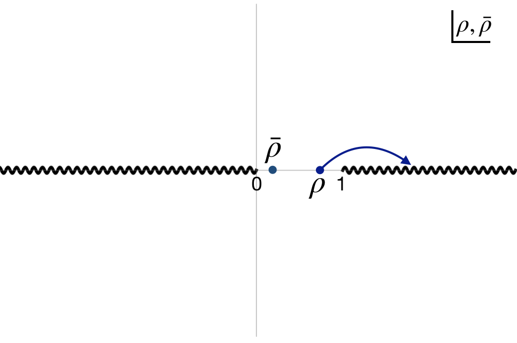
where, twist τp=Δp−ℓp\tau_{p}=\Delta_{p}-\ell_{p} and λp\lambda_{p} is a numerical coefficient exact value of which will not be important for us.77 7 The exact value of λp\lambda_{p} can be computed from the three-point function ⟨𝒪𝒪†𝒪μ1μ2⋯p⟩\langle{\cal O}{\cal O}^{\dagger}{\cal O}_{\mu_{1}\mu_{2}\cdots}^{p}\rangle λp=(−1)ℓp​c𝒪𝒪†​𝒪p​2Δp​Γ​(Δp+ℓp+12)cp​π​Γ​(Δp+ℓp2)2,\lambda_{p}=\frac{(-1)^{\ell_{p}}c_{{\cal O}{\cal O}^{\dagger}{\cal O}_{p}}2^{\Delta_{p}}\Gamma\left(\frac{\Delta_{p}+\ell_{p}+1}{2}\right)}{c_{p}\sqrt{\pi}\Gamma\left(\frac{\Delta_{p}+\ell_{p}}{2}\right)^{2}}\ , where, cpc_{p} is the coefficient of the two-point function of 𝒪μ1μ2⋯p{\cal O}_{\mu_{1}\mu_{2}\cdots}^{p}. Note that for real scalar primaries only operators with even spins can appear in the OPE. Hence, the factor of (−1)ℓp(-1)^{\ell_{p}} is not there in [10] for real scalars. This lightcone OPE can be used inside arbitrary correlators. In particular, we can use this OPE to derive the contribution of the 𝒪𝒪†→𝒪p→X​X¯{\cal O}{\cal O}^{\dagger}\rightarrow{\cal O}_{p}\rightarrow X\overline{X} conformal block to the correlator ⟨X⁡(𝟏)​𝒪​(𝝆)​𝒪⁡(𝝆)¯​X⁡(𝟏)¯⟩\langle X(\mathbf{1}){\cal O}(\text{\boldmath$\rho$})\overline{{\cal O}(\text{\boldmath$\rho$})}\ \overline{X(\mathbf{1})}\rangle in the Lorentzian lightcone limit (3.5). This Lorentzian correlator can be obtained from the Euclidean one by analytically continuing ρ\rho along the path shown in figure 2. The corresponding contour for the ρ′\rho^{\prime}-integral follows directly from the way operators are ordered inside the correlator.88 8 See [10] for a detailed discussion.
Refer to caption
Figure 2: The Lorentzian correlator GG of (3.1) is obtained from the Euclidean correlator by analytically continuing ρ\rho along the blue path.

Of course, we intend to utilize the analyticity and positivity conditions (i) and (ii). Hence, it is more convenient to study the lightcone limit of normalized correlators G⁡(η,σ)G(\eta,\sigma) and G0​(η,σ)G_{0}(\eta,\sigma), as defined in (3.1), using variables (3.3). In these variables, the Lorentzian lightcone limit (3.5) can be equivalently defined as 0<η≪|σ|≪10<\eta\ll|\sigma|\ll 1. As an immediate consequence of the lightcone OPE (3.7), we can write the contribution of the operator 𝒪p{\cal O}_{p} to G⁡(η,σ)−G0​(η,σ)G(\eta,\sigma)-G_{0}(\eta,\sigma) in the Lorentzian lightcone limit as an expansion

G⁡(η,σ)|𝒪p−G0​(η,σ)|𝒪p=i​ητp2σℓp−1​(Cℓp,ℓp+∑n=2,4,⋯Cℓp,ℓp−n​σn)+⋯,\displaystyle G(\eta,\sigma)|_{{\cal O}_{p}}-G_{0}(\eta,\sigma)|_{{\cal O}_{p}}=i\frac{\eta^{\frac{\tau_{p}}{2}}}{\sigma^{\ell_{p}-1}}\left(C_{\ell_{p},\ell_{p}}+\sum_{n=2,4,\cdots}C_{\ell_{p},\ell_{p}-n}\sigma^{n}\right)+\cdots\ , (3.8)

where dots represent correction terms that are either suppressed by higher powers of η\eta or decay for small σ\sigma. Notice that the sum in the above equation is only over even integers. Moreover, coefficients Cℓp,ℓ′C_{\ell_{p},\ell^{\prime}} are real which can be computed from the lightcone OPE (3.7). For example

Cℓp,ℓp=λp​Im⟨X(𝟏)∫−∞∞dρ′𝒪p−−⋯−(ρ′,0,0→)X⁡(𝟏)¯⟩⟨X⁡(𝟏)​X⁡(𝟏)¯⟩C_{\ell_{p},\ell_{p}}=\lambda_{p}\frac{\mbox{Im}\ \langle X(\mathbf{1})\int_{-\infty}^{\infty}d\rho^{\prime}{\cal O}^{p}_{--\cdots-}(\rho^{\prime},0,\vec{0})\overline{X(\mathbf{1})}\rangle}{\langle X(\mathbf{1})\overline{X(\mathbf{1})}\rangle} (3.9)

which is nonzero by definition and all other coefficients Cℓp,ℓ′∝Cℓp,ℓpC_{\ell_{p},\ell^{\prime}}\propto C_{\ell_{p},\ell_{p}}. Since, however, these coefficients do not depend on η\eta or σ\sigma, their actual values are not important to us.

By using the i​ϵi\epsilon prescription we can convince ourselves that that we do not need to cross any branch cuts to obtain a Rindler reflection symmetric correlator, even when some of the operators are time-like separated. Hence, the correlator G0​(η,σ)G_{0}(\eta,\sigma) can be computed by using the Euclidean OPE. This implies that G0​(η,σ)G_{0}(\eta,\sigma) is trivial in the lightcone limit (3.5) where it is dominated by the identity exchange

G0​(η,σ)=1+⋯,G_{0}(\eta,\sigma)=1+\cdots\ , (3.10)

where dots represent correction terms that are suppressed by positive powers of η\eta and σ\sigma.

The 𝒪𝒪†{\cal O}{\cal O}^{\dagger} OPE converges only when all operators are spacelike separated in a correlator. On the other hand, the 𝒪𝒪†{\cal O}{\cal O}^{\dagger} OPE in a Lorentzian correlator such as G⁡(η,σ)G(\eta,\sigma) may diverge. Notice that contributions of individual operators in (3.8) become increasingly singular with increasing spin which is a manifestation of the fact that the lightcone OPE (3.7) does not converge on the second sheet. However, by considering scalar four-point functions it was argued in [24] that the second sheet conformal blocks still can be trusted in the lightcone limit. The same argument applies in general implying any finite number of terms in the lightcone OPE on the second sheet produce a reliable asymptotic expansion in the limit η→0\eta\rightarrow 0 [10]. Hence, G⁡(η,σ)G(\eta,\sigma) in the Lorentzian lightcone limit can be expressed as a divergent asymptotic series which is organized by twist99 9 In the equation (3.11), we have ignored terms that decay for small σ\sigma. Any term in G⁡(η,σ)G(\eta,\sigma) that decay for small σ\sigma can be subtracted by analytically continuing G0​(η,σ)G_{0}(\eta,\sigma) appropriately and hence these terms do not play any role in our argument. This has been explained in detail in appendix A.

G⁡(η,σ)∼G0​(η,σ)+i​∑τp≤τc​u​t​o​f​fητp2σℓp−1​(Cℓp,ℓp+∑n=2,4,⋯Cℓp,ℓp−n​σn+⋯),G(\eta,\sigma)\sim G_{0}(\eta,\sigma)+i\sum_{\tau_{p}\leq\tau_{cutoff}}\frac{\eta^{\frac{\tau_{p}}{2}}}{\sigma^{\ell_{p}-1}}\left(C_{\ell_{p},\ell_{p}}+\sum_{n=2,4,\cdots}C_{\ell_{p},\ell_{p}-n}\sigma^{n}+\cdots\right)\ , (3.11)

where, dots represent terms that are suppressed by positive powers of both η\eta and σ\sigma. The spectrum of operators that appear both in the OPE 𝒪𝒪†{\cal O}{\cal O}^{\dagger} and X​X¯X\overline{X} can have an accumulation point in the twist. In that case, it is generally expected that the above asymptotic expansion is not valid beyond the accumulation point in the twist spectrum.

3.2 Nachtmann Theorem in CFT

We now have all the ingredients to derive and generalize the CFT Nachtmann theorem. Our starting point is the correlator ⟨X⁡(𝟏)​𝒪​(𝝆)​𝒪⁡(𝝆)¯​X⁡(𝟏)¯⟩\langle X(\mathbf{1}){\cal O}(\text{\boldmath$\rho$})\overline{{\cal O}(\text{\boldmath$\rho$})}\ \overline{X(\mathbf{1})}\rangle, where 𝒪{\cal O} is a scalar primary and XX is a completely arbitrary operator. The lightcone limit of this conformal four-point function, as we learned from equation (3.11), is an expansion in twist. So, in this limit only the family of minimal twist operators is important.

The family of minimal twist operators is defined in the usual way. In the present context, consider all spin ℓ\ell operators that appear in the OPE of both 𝒪𝒪†{\cal O}{\cal O}^{\dagger} and X​X¯X\overline{X}. Among these operators, we pick the operator 𝒪~ℓ\tilde{{\cal O}}_{\ell} which has the lowest twist. The family of minimal twist operators is then defined as {𝒪~ℓ|ℓ∈ℤ≥}\{\tilde{{\cal O}}_{\ell}\ |\ \ell\in{\mathbb{Z}}^{\geq}\}. We adopt the notation τ~ℓ\tilde{\tau}_{\ell} to denote the twist of 𝒪~ℓ\tilde{{\cal O}}_{\ell}.

Clearly, the spectrum of operators that appear in the OPE of both 𝒪𝒪†{\cal O}{\cal O}^{\dagger} and X​X¯X\overline{X} can have both even and odd spins when 𝒪{\cal O} is a complex scalar. In that case, it is more convenient to discuss the even and odd (spin) family of minimal twist operators separately.

Refer to caption
Figure 3: The integration contour in the complex-σ\sigma plane.

First, we derive a general sum rule by integrating δ​G​(η,σ)\delta G(\eta,\sigma), where

δ​G​(η,σ)≡G0​(η,σ)−G⁡(η,σ).\delta G(\eta,\sigma)\equiv G_{0}(\eta,\sigma)-G(\eta,\sigma)\ . (3.12)

As in [10], we choose an integration contour which is a half-disk near σ=0\sigma=0, just below the real line in the complex-σ\sigma plane (see figure 3). The radius RR of the semicircle is such that it satisfies η≪R≪1\eta\ll R\ll 1. Strictly speaking, G0​(η,σ)G_{0}(\eta,\sigma) is only defined on the real line. However, we can still define a function G0(−)​(η,σ)G_{0}^{(-)}(\eta,\sigma) which is analytic on the lower half σ\sigma-plane and has the property Re​G0(−)​(η,σ)=G0​(η,σ)\mbox{Re}\ G_{0}^{(-)}(\eta,\sigma)=G_{0}(\eta,\sigma) (for a detailed discussion see appendix A). The analyticity property (i) then requires that

Re​∮d​σ​σn​(G0(−)​(η,σ)−G⁡(η,σ))=0\mbox{Re}\oint d\sigma\ \sigma^{n}\left(G_{0}^{(-)}(\eta,\sigma)-G(\eta,\sigma)\right)=0\ (3.13)

for integer n≥0n\geq 0. The above contour integral can be divided into two parts – one over the real line and one over the semicircle. The lightcone limit expression (3.8) is valid over the entire semicircle. Moreover, the semicircle integral can be further and crucially simplified using the identity

Re​i​∫Sd​σ​σn=π​δn,−1,\mbox{Re}\ i\int_{S}d\sigma\sigma^{n}=\pi\delta_{n,-1}\ , (3.14)

where, S={R​ei​θ,θ∈[0,−π]}S=\{Re^{i\theta},\theta\in[0,-\pi]\}. This enables us to write a sum rule

∑ℓ′≥ℓCℓ′,ℓ​ητ~ℓ′2=1π​∫−RRd​σ​σℓ−2​Re​(δ​G​(η,σ)),integer​ℓ≥2\sum_{\ell^{\prime}\geq\ell}C_{\ell^{\prime},\ell}\ \eta^{\frac{\tilde{\tau}_{\ell^{\prime}}}{2}}=\frac{1}{\pi}\int_{-R}^{R}d\sigma\ \sigma^{\ell-2}\mbox{Re}(\delta G(\eta,\sigma))\ ,\qquad\text{integer}\ \ell\geq 2 (3.15)

where 0<η≪R≪10<\eta\ll R\ll 1. The left hand side of the above relation is written as a formal sum which reflects the fact that any operator 𝒪~ℓ′\tilde{{\cal O}}_{\ell^{\prime}} with ℓ′=ℓ+2​N\ell^{\prime}=\ell+2N (for non-negative integer NN) can contribute to the correlator G⁡(η,σ)G(\eta,\sigma) a term that grows exactly as 1σℓ−1\frac{1}{\sigma^{\ell-1}} in the Lorentzian lightcone limit. However, it should be understood that for any ℓ\ell only the term (or terms) with the lowest τ~ℓ′\tilde{\tau}_{\ell^{\prime}} dominates.

The observant reader may have noticed that dots in equation (3.8) contain terms that decay with positive but non-integer powers of σ\sigma when operators with non-integer dimensions are exchanged. These terms appear to spoil the projection to a specific power of 1σ\frac{1}{\sigma} by using the identity (3.14). However, these terms do not actually contribute to the sum rule (3.15), since these terms get exactly canceled by G0(−)​(η,σ)G_{0}^{(-)}(\eta,\sigma). This is explained in detail in appendix A.

Next we use the sum rule (3.15) to derive the monotonicity and convexity properties of the even spin family of minimal twist operators.

Monotonicity

The positivity condition (ii) immediately implies that the left hand side of (3.15) must be non-negative for any even ℓ\ell.1010 10 Strictly speaking, the inequality (3.4) is valid only for real σ\sigma. There is a complexified version of Rindler positivity, as discussed in [10], which implies (3.4) on the straight line part of the contour 3 even when it lies just below the real axis in the complex-σ\sigma plane. Furthermore, the positivity condition (ii) also leads to the following inequality for any two even ℓ2>ℓ1≥2\ell_{2}>\ell_{1}\geq 2

∫−RRd​σ​σℓ2−2​Re​(δ​G​(η,σ))∫−RRd​σ​σℓ1−2​Re​(δ​G​(η,σ))≤Rℓ2−ℓ1≪1.\frac{\int_{-R}^{R}d\sigma\ \sigma^{\ell_{2}-2}\mbox{Re}(\delta G(\eta,\sigma))}{\int_{-R}^{R}d\sigma\ \sigma^{\ell_{1}-2}\mbox{Re}(\delta G(\eta,\sigma))}\leq R^{\ell_{2}-\ell_{1}}\ll 1\ . (3.16)

Hence, the sum rule (3.15) implies that

∑ℓ′≥ℓ2Cℓ′,ℓ2​ητ~ℓ′2∑ℓ′≥ℓ1Cℓ′,ℓ1​ητ~ℓ′2≪1\frac{\sum_{\ell^{\prime}\geq\ell_{2}}C_{\ell^{\prime},\ell_{2}}\ \eta^{\frac{\tilde{\tau}_{\ell^{\prime}}}{2}}}{\sum_{\ell^{\prime}\geq\ell_{1}}C_{\ell^{\prime},\ell_{1}}\ \eta^{\frac{\tilde{\tau}_{\ell^{\prime}}}{2}}}\ll 1

in the limit η→0\eta\rightarrow 0. Since, Cℓ,ℓ′C_{\ell,\ell^{\prime}} do not scale with η\eta, the above inequality can be satisfied iff

τ~ℓ2≥τ~ℓ1,ℓ2>ℓ1≥2\tilde{\tau}_{\ell_{2}}\geq\tilde{\tau}_{\ell_{1}}\ ,\qquad\ell_{2}>\ell_{1}\geq 2\ (3.17)

for all even ℓ1\ell_{1} and ℓ2\ell_{2}. The equality in the above relation holds only for free CFTs and 2d CFTs. In these CFTs, the relation (3.17) is trivially satisfied since they contain an infinite tower of higher spin conserved currents.

The monotonicity condition (3.17) greatly simplifies the sum rule (3.15) for interacting CFTs in d>2d>2 dimensions. For any even ℓ\ell, clearly the first term Cℓ,ℓ​ητ~ℓ2C_{\ell,\ell}\eta^{\frac{\tilde{\tau}_{\ell}}{2}} dominates in the left hand side implying three-point functions

Cℓ,ℓ>0for even ℓ≥2C_{\ell,\ell}>0\qquad\text{for even $\ell\geq 2$} (3.18)

which is consistent with the averaged null energy condition and its higher spin generalization as derived in [10].

Convexity

Similar to [6], we can actually derive a stronger constraint on the family of minimal twist operators with even spins. For any even ℓ≥2\ell\geq 2, the Cauchy-Schwarz inequality of real integrable functions imposes

0<(∫−RRd​σ​σℓ​Re​(δ​G​(η,σ)))2∫−RRd​σ​σℓ−2​Re​(δ​G​(η,σ))​∫−RRd​σ​σℓ+2​Re​(δ​G​(η,σ))≤1.0<\frac{\left(\int_{-R}^{R}d\sigma\ \sigma^{\ell}\mbox{Re}(\delta G(\eta,\sigma))\right)^{2}}{\int_{-R}^{R}d\sigma\ \sigma^{\ell-2}\mbox{Re}(\delta G(\eta,\sigma))\int_{-R}^{R}d\sigma\ \sigma^{\ell+2}\mbox{Re}(\delta G(\eta,\sigma))}\leq 1\ . (3.19)

In the regime 0<η≪R≪10<\eta\ll R\ll 1, we can use the sum rule (3.15) and the monotonicity condition (3.17) to rewrite the above inequality as

0<limη→0(Cℓ+2,ℓ+22Cℓ,ℓ​Cℓ+4,ℓ+4)​η12​(2​τ~ℓ+2−τ~ℓ−τ~ℓ+4)≤10<\lim_{\eta\rightarrow 0}\left(\frac{C_{\ell+2,\ell+2}^{2}}{C_{\ell,\ell}C_{\ell+4,\ell+4}}\right)\eta^{\frac{1}{2}\left(2\tilde{\tau}_{\ell+2}-\tilde{\tau}_{\ell}-\tilde{\tau}_{\ell+4}\right)}\leq 1 (3.20)

implying 2​τ~ℓ+2≥τ~ℓ+τ~ℓ+42\tilde{\tau}_{\ell+2}\geq\tilde{\tau}_{\ell}+\tilde{\tau}_{\ell+4} for any even ℓ≥2\ell\geq 2. This local convexity condition can be applied iteratively to obtain

τ~ℓ3−τ~ℓ1ℓ3−ℓ1≤τ~ℓ2−τ~ℓ1ℓ2−ℓ1,2≤ℓ1<ℓ2<ℓ3\frac{\tilde{\tau}_{\ell_{3}}-\tilde{\tau}_{\ell_{1}}}{\ell_{3}-\ell_{1}}\leq\frac{\tilde{\tau}_{\ell_{2}}-\tilde{\tau}_{\ell_{1}}}{\ell_{2}-\ell_{1}}\ ,\qquad 2\leq\ell_{1}<\ell_{2}<\ell_{3} (3.21)

for all even ℓ1\ell_{1}, ℓ2\ell_{2} and ℓ3\ell_{3}.

To summarize, twist is a monotonically increasing convex function of the spin for the even (spin) family of minimal twist operators appearing in the OPE of both 𝒪𝒪†{\cal O}{\cal O}^{\dagger} and X​X¯X\overline{X}, where 𝒪{\cal O} is a scalar primary and XX is a completely arbitrary operator with or without spin (not necessarily local or primary) in any interacting unitary CFT in d≥3d\geq 3 dimensions. This is, in general, stronger than the convexity theorem of [6] (with ℓc=2\ell_{c}=2). In particular, different choices of XX can lead to different families of minimal twist operators and the conditions (3.17) and (3.21) apply to each such family. For example, in theories with global symmetries, the OPE 𝒪𝒪†{\cal O}{\cal O}^{\dagger} may contain several different families of operators that obey the monotonicity and the convexity conditions.

Family of minimal twist operators with odd spins

Let us now move on to minimal twist operators with odd spins. This discussion is relevant only when 𝒪{\cal O} is complex. Clearly, the integrand in (3.15) is not strictly positive for odd ℓ\ell. Hence, the family of minimal twist operators with odd spins does not in general obey the monotonicity and the convexity conditions. This should not be surprising since there are known examples that would violate any such conditions [25]. However, it is not true that the family of minimal twist operators with odd spins is completely free of constraints. For any even ℓe\ell_{e} and odd ℓo\ell_{o} satisfying ℓo>ℓe≥2\ell_{o}>\ell_{e}\geq 2, the positivity condition (ii) imposes

|∑ℓ′≥ℓoCℓ′,ℓo​ητ~ℓ′2|Cℓe,ℓe​ητ~ℓe2=|∫−RRd​σ​σℓo−2​Re​(δ​G​(η,σ))|∫−RRd​σ​σℓe−2​Re​(δ​G​(η,σ))≤Rℓo−ℓe≪1\frac{|\sum_{\ell^{\prime}\geq\ell_{o}}C_{\ell^{\prime},\ell_{o}}\ \eta^{\frac{\tilde{\tau}_{\ell^{\prime}}}{2}}|}{C_{\ell_{e},\ell_{e}}\ \eta^{\frac{\tilde{\tau}_{\ell_{e}}}{2}}}=\frac{|\int_{-R}^{R}d\sigma\ \sigma^{\ell_{o}-2}\mbox{Re}(\delta G(\eta,\sigma))|}{\int_{-R}^{R}d\sigma\ \sigma^{\ell_{e}-2}\mbox{Re}(\delta G(\eta,\sigma))}\leq R^{\ell_{o}-\ell_{e}}\ll 1\ (3.22)

implying

τ~ℓo>τ~ℓe,for allℓo>ℓe≥2.\tilde{\tau}_{\ell_{o}}>\tilde{\tau}_{\ell_{e}}\ ,\qquad\text{for all}\qquad\ell_{o}>\ell_{e}\geq 2\ . (3.23)

On the other hand, twists of two odd spin minimal twist operators do not obey any such condition.

Odd spin minimal twist operators also satisfy a local convexity condition. For any odd ℓ0≥3\ell_{0}\geq 3, the Cauchy-Schwarz inequality can be utilized to write

0<(∫−RRd​σ​σℓo−2​Re​(δ​G​(η,σ)))2∫−RRd​σ​σℓo−3​Re​(δ​G​(η,σ))​∫−RRd​σ​σℓo−1​Re​(δ​G​(η,σ))≤1.0<\frac{\left(\int_{-R}^{R}d\sigma\ \sigma^{\ell_{o}-2}\mbox{Re}(\delta G(\eta,\sigma))\right)^{2}}{\int_{-R}^{R}d\sigma\ \sigma^{\ell_{o}-3}\mbox{Re}(\delta G(\eta,\sigma))\int_{-R}^{R}d\sigma\ \sigma^{\ell_{o}-1}\mbox{Re}(\delta G(\eta,\sigma))}\leq 1\ . (3.24)

In the regime 0<η≪R≪10<\eta\ll R\ll 1, we can use the sum rule (3.15) and the condition (3.23) to obtain a local convexity condition for any odd ℓo≥3\ell_{o}\geq 3

τ~ℓo≥τ~ℓo−1+τ~ℓo+12.\tilde{\tau}_{\ell_{o}}\geq\frac{\tilde{\tau}_{\ell_{o}-1}+\tilde{\tau}_{\ell_{o}+1}}{2}\ . (3.25)

Note that this condition is stronger than (3.23). Finally, we can apply this local convexity condition iteratively to obtain

τ~ℓo−τ~ℓeℓo−ℓe≥τ~ℓe′−τ~ℓeℓe′−ℓe,2≤ℓe<ℓo<ℓe′\frac{\tilde{\tau}_{\ell_{o}}-\tilde{\tau}_{\ell_{e}}}{\ell_{o}-\ell_{e}}\geq\frac{\tilde{\tau}_{\ell_{e}^{\prime}}-\tilde{\tau}_{\ell_{e}}}{\ell_{e}^{\prime}-\ell_{e}}\ ,\qquad 2\leq\ell_{e}<\ell_{o}<\ell_{e}^{\prime} (3.26)

for all even ℓe\ell_{e}, ℓe′\ell_{e}^{\prime} and odd ℓo\ell_{o}. In contrast to (3.21), the condition (3.26) only provides a lower bound on τ~ℓo\tilde{\tau}_{\ell_{o}} for ℓo≥3\ell_{o}\geq 3 implying that the family of minimal twist operators with odd spins do not, in general, obey any global convexity condition.

It is possible that there are a stronger bounds on odd spin minimal twist operators. For example, there may be some relation between the continuous even spin and odd spin leading Regge trajectories above ℓ>1\ell>1. We believe that such a relation, if it exists, can be derived by combining our method with the Lorentzian inversion formula.

To summarize, we rederived and extended the convexity theorem of [6] by using analyticity and positivity properties of CFT correlators in Lorentzian signature. We end this section by commenting on a possible limitation of our argument. If the spectrum of operators that appears both in the OPE 𝒪𝒪†{\cal O}{\cal O}^{\dagger} and X​X¯X\overline{X} have an accumulation point in the twist at τ∗\tau_{*}, it is not clear if our derivation is valid beyond τ~ℓ>τ∗\tilde{\tau}_{\ell}>\tau_{*}.

4 OPE of Nonidentical Operators

It is only natural to wonder if the preceding analysis can be extended to OPEs of nonidentical scalar primaries in unitary CFTs. As the discussion of section 2 leads us to expect, the family of minimal twist operators appearing in the OPE of nonidentical scalar primaries does obey some general constraints which we will discuss next. Before we proceed, we introduce the notation

δ⁡⟨𝒪I​(𝟏)​𝒪J​(𝝆)​𝒪K​(−𝝆)​𝒪L​(−𝟏)⟩=\displaystyle\delta\langle{\cal O}_{I}(\mathbf{1}){\cal O}_{J}(\text{\boldmath$\rho$}){\cal O}_{K}(-\text{\boldmath$\rho$}){\cal O}_{L}(-\mathbf{1})\rangle= ⟨𝒪I​(𝟏)​𝒪J​(𝝆)​𝒪K​(−𝟏)​𝒪L​(−𝝆)⟩\displaystyle\langle{\cal O}_{I}(\mathbf{1}){\cal O}_{J}(\text{\boldmath$\rho$}){\cal O}_{K}(-\mathbf{1}){\cal O}_{L}(-\text{\boldmath$\rho$})\rangle
−⟨𝒪I​(𝟏)​𝒪J​(𝝆)​𝒪K​(−𝝆)​𝒪L​(−𝟏)⟩,\displaystyle-\langle{\cal O}_{I}(\mathbf{1}){\cal O}_{J}(\text{\boldmath$\rho$}){\cal O}_{K}(-\text{\boldmath$\rho$}){\cal O}_{L}(-\mathbf{1})\rangle\ , (4.1)

where operators are ordered as written. As remarked before, we do not need to cross any branch cuts to obtain the Lorentzian correlator ⟨𝒪I​(𝟏)​𝒪J​(𝝆)​𝒪K​(−𝟏)​𝒪L​(−𝝆)⟩\langle{\cal O}_{I}(\mathbf{1}){\cal O}_{J}(\text{\boldmath$\rho$}){\cal O}_{K}(-\mathbf{1}){\cal O}_{L}(-\text{\boldmath$\rho$})\rangle and hence this correlators can be determined by using the Euclidean OPE even for ρ>1\rho>1. Clearly, the same argument holds for the Lorentzian correlator ⟨𝒪J​(𝝆)​𝒪I​(𝟏)​𝒪L​(−𝝆)​𝒪K​(−𝟏)⟩\langle{\cal O}_{J}(\text{\boldmath$\rho$}){\cal O}_{I}(\mathbf{1}){\cal O}_{L}(-\text{\boldmath$\rho$}){\cal O}_{K}(-\mathbf{1})\rangle as well which implies that ⟨𝒪I​(𝟏)​𝒪J​(𝝆)​𝒪K​(−𝟏)​𝒪L​(−𝝆)=⟨𝒪J​(𝝆)​𝒪I​(𝟏)​𝒪L​(−𝝆)​𝒪K​(−𝟏)⟩⟩\langle{\cal O}_{I}(\mathbf{1}){\cal O}_{J}(\text{\boldmath$\rho$}){\cal O}_{K}(-\mathbf{1}){\cal O}_{L}(-\text{\boldmath$\rho$})=\langle{\cal O}_{J}(\text{\boldmath$\rho$}){\cal O}_{I}(\mathbf{1}){\cal O}_{L}(-\text{\boldmath$\rho$}){\cal O}_{K}(-\mathbf{1})\rangle\rangle even when ρ>1\rho>1.

4.1 Mixed Correlators and Rindler Positivity

A Nachtmann-like theorem for nonidentical scalar primaries requires a condition similar to (3.4) for the mixed correlator ⟨𝒪2†​(𝟏)​𝒪1​(𝝆)​𝒪2​(−𝝆)​𝒪1†​(−𝟏)⟩\langle{\cal O}_{2}^{\dagger}(\mathbf{1}){\cal O}_{1}(\text{\boldmath$\rho$}){\cal O}_{2}(-\text{\boldmath$\rho$}){\cal O}_{1}^{\dagger}(-\mathbf{1})\rangle. In unitary Lorentzian QFTs, such a condition can be derived by utilizing Rindler positivity. Consider two operators AA and BB with support in the left Rindler wedge. We can define a positive inner product (A,B)≡⟨B​A¯⟩+⟨A​B¯⟩(A,B)\equiv\langle B\overline{A}\rangle+\langle A\overline{B}\rangle by using Rindler positivity. This comes with the Cauchy-Schwarz identity

(A,B)2≤(A,A)​(B,B).(A,B)^{2}\leq(A,A)(B,B)\ . (4.2)

Inequality I

Now consider two scalar primaries 𝒪1{\cal O}_{1} and 𝒪2{\cal O}_{2} with dimensions Δ1\Delta_{1} and Δ2\Delta_{2} respectively. First, we choose

A\displaystyle A =(ρ​ρ¯)Δ2+δ22​𝒪1​(𝟏)​𝒪2†​(𝝆)±(ρ​ρ¯)Δ1+δ12​𝒪2†​(𝟏)​𝒪1​(𝝆),\displaystyle=(\rho\bar{\rho})^{\frac{\Delta_{2}+\delta_{2}}{2}}{\cal O}_{1}(\mathbf{1}){\cal O}_{2}^{\dagger}(\text{\boldmath$\rho$})\pm(\rho\bar{\rho})^{\frac{\Delta_{1}+\delta_{1}}{2}}{\cal O}_{2}^{\dagger}(\mathbf{1}){\cal O}_{1}(\text{\boldmath$\rho$})\ ,
B\displaystyle B =±(ρ​ρ¯)Δ1+δ12​𝒪1​(𝝆)​𝒪2†​(𝟏)+(ρ​ρ¯)Δ2+δ22​𝒪2†​(𝝆)​𝒪1​(𝟏),\displaystyle=\pm(\rho\bar{\rho})^{\frac{\Delta_{1}+\delta_{1}}{2}}{\cal O}_{1}(\text{\boldmath$\rho$}){\cal O}_{2}^{\dagger}(\mathbf{1})+(\rho\bar{\rho})^{\frac{\Delta_{2}+\delta_{2}}{2}}{\cal O}_{2}^{\dagger}(\text{\boldmath$\rho$}){\cal O}_{1}(\mathbf{1})\ , (4.3)

where δ1\delta_{1} and δ2\delta_{2} are arbitrary real numbers that we will fix later. The Cauchy-Schwarz identity (4.2) now leads to an inequality which applies to any unitary QFT. This inequality can be further simplified for CFTs where some of the correlators are related because of conformal symmetry. Specifically for 0<ρ¯​<1,ρ>​10<\bar{\rho}<1,\ \rho>1 we obtain1111 11 Note that we are using the notation (4).

±2​Re​δ​⟨𝒪2†​(𝟏)​𝒪1​(𝝆)​𝒪2​(−𝝆)​𝒪1†​(−𝟏)⟩≤(ρ​ρ¯)Δ21+δ212\displaystyle\pm 2\mbox{Re}\ \delta\langle{\cal O}_{2}^{\dagger}(\mathbf{1}){\cal O}_{1}(\text{\boldmath$\rho$}){\cal O}_{2}(-\text{\boldmath$\rho$}){\cal O}_{1}^{\dagger}(-\mathbf{1})\rangle\leq(\rho\bar{\rho})^{\frac{\Delta_{21}+\delta_{21}}{2}} Re​δ​⟨𝒪1†​(𝟏)​𝒪2​(𝝆)​𝒪2†​(−𝝆)​𝒪1​(−𝟏)⟩\displaystyle\mbox{Re}\ \delta\langle{\cal O}_{1}^{\dagger}(\mathbf{1}){\cal O}_{2}(\text{\boldmath$\rho$}){\cal O}_{2}^{\dagger}(-\text{\boldmath$\rho$}){\cal O}_{1}(-\mathbf{1})\rangle
+(ρ​ρ¯)−Δ21+δ212​Re​δ\displaystyle+(\rho\bar{\rho})^{-\frac{\Delta_{21}+\delta_{21}}{2}}\mbox{Re}\ \delta ⟨𝒪2†​(𝟏)​𝒪1​(𝝆)​𝒪1†​(−𝝆)​𝒪2​(−𝟏)⟩\displaystyle\langle{\cal O}_{2}^{\dagger}(\mathbf{1}){\cal O}_{1}(\text{\boldmath$\rho$}){\cal O}_{1}^{\dagger}(-\text{\boldmath$\rho$}){\cal O}_{2}(-\mathbf{1})\rangle\ (4.4)

for any real δ1\delta_{1} and δ2\delta_{2}, where operators inside correlators are ordered as written. In the above equation, we have defined Δ21=Δ2−Δ1\Delta_{21}=\Delta_{2}-\Delta_{1} and δ21=δ2−δ1\delta_{21}=\delta_{2}-\delta_{1}.

Inequality II

Likewise, we can derive a similar inequality for a different mixed correlator by choosing

A\displaystyle A =(ρ​ρ¯)Δ1+δ12​𝒪1​(𝟏)​𝒪1†​(𝝆)±(ρ​ρ¯)Δ2+δ22​𝒪2†​(𝟏)​𝒪2​(𝝆),\displaystyle=(\rho\bar{\rho})^{\frac{\Delta_{1}+\delta_{1}}{2}}{\cal O}_{1}(\mathbf{1}){\cal O}_{1}^{\dagger}(\text{\boldmath$\rho$})\pm(\rho\bar{\rho})^{\frac{\Delta_{2}+\delta_{2}}{2}}{\cal O}_{2}^{\dagger}(\mathbf{1}){\cal O}_{2}(\text{\boldmath$\rho$})\ ,
B\displaystyle B =(ρ​ρ¯)Δ1+δ12​𝒪1†​(𝝆)​𝒪1​(𝟏)±(ρ​ρ¯)Δ2+δ22​𝒪2​(𝝆)​𝒪2†​(𝟏).\displaystyle=(\rho\bar{\rho})^{\frac{\Delta_{1}+\delta_{1}}{2}}{\cal O}_{1}^{\dagger}(\text{\boldmath$\rho$}){\cal O}_{1}(\mathbf{1})\pm(\rho\bar{\rho})^{\frac{\Delta_{2}+\delta_{2}}{2}}{\cal O}_{2}(\text{\boldmath$\rho$}){\cal O}_{2}^{\dagger}(\mathbf{1})\ . (4.5)

For 0<ρ¯​<1,ρ>​10<\bar{\rho}<1,\ \rho>1, the Cauchy-Schwarz identity (4.2) imposes

±2Reδ⟨𝒪2†(𝟏)𝒪2(𝝆)𝒪1(−𝝆)\displaystyle\pm 2\mbox{Re}\ \delta\langle{\cal O}_{2}^{\dagger}(\mathbf{1}){\cal O}_{2}(\text{\boldmath$\rho$}){\cal O}_{1}(-\text{\boldmath$\rho$}) 𝒪1†(−𝟏)⟩≤(ρρ¯)−Δ21+δ212Reδ⟨𝒪1†(𝟏)𝒪1(𝝆)𝒪1†(−𝝆)𝒪1(−𝟏)⟩\displaystyle{\cal O}_{1}^{\dagger}(-\mathbf{1})\rangle\leq(\rho\bar{\rho})^{-\frac{\Delta_{21}+\delta_{21}}{2}}\mbox{Re}\ \delta\langle{\cal O}_{1}^{\dagger}(\mathbf{1}){\cal O}_{1}(\text{\boldmath$\rho$}){\cal O}_{1}^{\dagger}(-\text{\boldmath$\rho$}){\cal O}_{1}(-\mathbf{1})\rangle
+(ρ​ρ¯)Δ21+δ212​Re​δ​⟨𝒪2†​(𝟏)​𝒪2​(𝝆)​𝒪2†​(−𝝆)​𝒪2​(−𝟏)⟩\displaystyle+(\rho\bar{\rho})^{\frac{\Delta_{21}+\delta_{21}}{2}}\mbox{Re}\ \delta\langle{\cal O}_{2}^{\dagger}(\mathbf{1}){\cal O}_{2}(\text{\boldmath$\rho$}){\cal O}_{2}^{\dagger}(-\text{\boldmath$\rho$}){\cal O}_{2}(-\mathbf{1})\rangle\ (4.6)

for any real δ1\delta_{1} and δ2\delta_{2}. Of course, the above argument holds for any unitary QFT. However, conformal symmetry was used to simplify the Cauchy-Schwarz identity to obtain the final inequalities (4.1) and (4.1). So, for non-conformal QFTs, one must use the exact expression obtained from the Cauchy-Schwarz identity (4.2) for AA and BB given in (4.1) or (4.1).

The inequalities (4.1) and (4.1) together, as we explain below, impose constraints on the family of minimal twist operators appearing in the OPE 𝒪1​𝒪2{\cal O}_{1}{\cal O}_{2}. To derive any such constraint, first it is necessary to understand the Lorentzian lightcone limit of the mixed correlator ⟨𝒪2†​(𝟏)​𝒪1​(𝝆)​𝒪2​(−𝝆)​𝒪1†​(−𝟏)⟩\langle{\cal O}_{2}^{\dagger}(\mathbf{1}){\cal O}_{1}(\text{\boldmath$\rho$}){\cal O}_{2}(-\text{\boldmath$\rho$}){\cal O}_{1}^{\dagger}(-\mathbf{1})\rangle.

4.2 Lightcone OPE

It is straightforward to generalize the lightcone OPE of [10] for nonidentical scalar primaries. The contribution of the primary operator 𝒪pμ1μ2⋯{\cal O}^{p}_{\mu_{1}\mu_{2}\cdots} with conformal dimension Δp\Delta_{p} and spin ℓp\ell_{p} and its descendants to the OPE 𝒪1​𝒪2{\cal O}_{1}{\cal O}_{2} in the lightcone limit ρ​ρ¯→0\rho\bar{\rho}\rightarrow 0 can be written as

𝒪1(𝝆)𝒪2(−𝝆)|𝒪p=λ~p(ρ​ρ¯)τp2​ρℓp−1(2​ρ​ρ¯)Δ1+Δ22∫−ρρdρ′(1−ρ′ρ)−Δ12+hp−22(1+ρ′ρ)Δ12+hp−22𝒪−⋯−p(ρ′)\displaystyle{\cal O}_{1}(\text{\boldmath$\rho$}){\cal O}_{2}(-\text{\boldmath$\rho$})|_{{\cal O}_{p}}=\tilde{\lambda}_{p}\frac{\left(\rho\bar{\rho}\right)^{\frac{\tau_{p}}{2}}\rho^{\ell_{p}-1}}{(2\rho\bar{\rho})^{\frac{\Delta_{1}+\Delta_{2}}{2}}}\int_{-\rho}^{\rho}d\rho^{\prime}\left(1-\frac{{\rho^{\prime}}}{\rho}\right)^{\frac{-\Delta_{12}+h_{p}-2}{2}}\left(1+\frac{{\rho^{\prime}}}{\rho}\right)^{\frac{\Delta_{12}+h_{p}-2}{2}}{\cal O}^{p}_{-\cdots-}(\rho^{\prime}) (4.7)

where, hp=Δp+ℓph_{p}=\Delta_{p}+\ell_{p} and twist τp=Δp−ℓp\tau_{p}=\Delta_{p}-\ell_{p}. Actual value of the coefficient λ~p\tilde{\lambda}_{p} is not important for our purpose, however let us note it here anyway

λ~p=(−2)−ℓp​2​c𝒪1​𝒪2​𝒪p​Γ​(hp)cp​Γ​(12​(hp−Δ21))​Γ​(12​(hp+Δ21))\tilde{\lambda}_{p}=(-2)^{-\ell_{p}}\frac{2c_{{\cal O}_{1}{\cal O}_{2}{\cal O}_{p}}\Gamma\left(h_{p}\right)}{c_{p}\Gamma\left(\frac{1}{2}\left(h_{p}-\Delta_{21}\right)\right)\Gamma\left(\frac{1}{2}\left(h_{p}+\Delta_{21}\right)\right)} (4.8)

where, cpc_{p} is the coefficient of the two-point function of ⟨𝒪p​𝒪p⟩\langle{\cal O}_{p}{\cal O}_{p}\rangle.1212 12 See [26] for conventions. The lightcone OPE (4.7) allows us to derive the contribution of the 𝒪1​𝒪2→𝒪p→𝒪1†​𝒪2†{\cal O}_{1}{\cal O}_{2}\rightarrow{\cal O}_{p}\rightarrow{\cal O}_{1}^{\dagger}{\cal O}_{2}^{\dagger} conformal block to the correlator ⟨𝒪2†​(𝟏)​𝒪1​(𝝆)​𝒪2​(−𝝆)​𝒪1†​(−𝟏)⟩\langle{\cal O}_{2}^{\dagger}(\mathbf{1}){\cal O}_{1}(\text{\boldmath$\rho$}){\cal O}_{2}(-\text{\boldmath$\rho$}){\cal O}_{1}^{\dagger}(-\mathbf{1})\rangle (or any other related Lorentzian correlators) in the lightcone limit. In particular, in the Lorentzian lightcone limit 0<η≪|σ|≪10<\eta\ll|\sigma|\ll 1 we obtain1313 13 Variables η\eta and σ\sigma are defined in (3.3).

δ⁡⟨𝒪2†​(𝟏)​𝒪1​(𝝆)​𝒪2​(−𝝆)​𝒪1†​(−𝟏)⟩|𝒪p=−i​η12​(τp−Δ1−Δ2)σℓp−1​(C~ℓp,ℓp+∑n=1ℓp−1C~ℓp,ℓp−n​σn)\displaystyle\delta\langle{\cal O}_{2}^{\dagger}(\mathbf{1}){\cal O}_{1}(\text{\boldmath$\rho$}){\cal O}_{2}(-\text{\boldmath$\rho$}){\cal O}_{1}^{\dagger}(-\mathbf{1})\rangle|_{{\cal O}_{p}}=-i\frac{\eta^{\frac{1}{2}\left(\tau_{p}-\Delta_{1}-\Delta_{2}\right)}}{\sigma^{\ell_{p}-1}}\left(\tilde{C}_{\ell_{p},\ell_{p}}+\sum_{n=1}^{\ell_{p}-1}\tilde{C}_{\ell_{p},\ell_{p}-n}\sigma^{n}\right) (4.9)

plus correction terms that are either suppressed by higher powers of η\eta or decay for small σ\sigma. For our argument, as explained in appendix B, we can safely ignore these correction terms. In the above equation, actual values of coefficients C~ℓp,ℓ′∝|c𝒪1​𝒪2​𝒪p|2\tilde{C}_{\ell_{p},\ell^{\prime}}\propto|c_{{\cal O}_{1}{\cal O}_{2}{\cal O}_{p}}|^{2} are not important. These coefficients can be computed either from the OPE (4.7) or by using the lightcone conformal block derived by Dolan and Osborn in [27]. Finally, the mixed correlator in the Lorentzian lightcone limit can also be expressed as an asymptotic series which is organized by twist

δ⟨𝒪2†(𝟏)𝒪1(𝝆)𝒪2(−𝝆)𝒪1†(−𝟏)⟩∼−i∑τp≤τc​u​t​o​f​fη12​(τp−Δ1−Δ2)σℓp−1(C~ℓp,ℓp+∑n=1ℓp−1C~ℓp,ℓp−nσn).\delta\langle{\cal O}_{2}^{\dagger}(\mathbf{1}){\cal O}_{1}(\text{\boldmath$\rho$}){\cal O}_{2}(-\text{\boldmath$\rho$}){\cal O}_{1}^{\dagger}(-\mathbf{1})\rangle\sim-i\sum_{\tau_{p}\leq\tau_{cutoff}}\frac{\eta^{\frac{1}{2}\left(\tau_{p}-\Delta_{1}-\Delta_{2}\right)}}{\sigma^{\ell_{p}-1}}\left(\tilde{C}_{\ell_{p},\ell_{p}}+\sum_{n=1}^{\ell_{p}-1}\tilde{C}_{\ell_{p},\ell_{p}-n}\sigma^{n}\right)\ . (4.10)

4.3 Constraints on the Family of Minimal Twist Operators

x+x^{+}x−\ x^{-}𝒪2†​(𝟏)\ {\cal O}_{2}^{\dagger}(\mathbf{1})𝒪1†​(−𝟏){\cal O}_{1}^{\dagger}(-\mathbf{1})𝒪1​(𝝆){\cal O}_{1}(\text{\boldmath$\rho$})𝒪2​(−𝝆){\cal O}_{2}(-\text{\boldmath$\rho$})
Figure 4: A non-Rindler symmetric four-point function of two scalar primaries 𝒪1{\cal O}_{1} and 𝒪2{\cal O}_{2}.

We are now in a position to derive constraints on the family of minimal twist operators that appears in the OPE 𝒪1​𝒪2{\cal O}_{1}{\cal O}_{2}. Consider the mixed Lorentzian correlator

Gm​i​x​e​d​(η,σ)=η12​(Δ1+Δ2+δ1+δ2)​⟨𝒪2†​(𝟏)​𝒪1​(𝝆)​𝒪2​(−𝝆)​𝒪1†​(−𝟏)⟩\displaystyle G_{mixed}(\eta,\sigma)=\eta^{\frac{1}{2}\left(\Delta_{1}+\Delta_{2}+\delta_{1}+\delta_{2}\right)}\langle{\cal O}_{2}^{\dagger}(\mathbf{1}){\cal O}_{1}(\text{\boldmath$\rho$}){\cal O}_{2}(-\text{\boldmath$\rho$}){\cal O}_{1}^{\dagger}(-\mathbf{1})\rangle (4.11)

in a unitary CFT in d≥3d\geq 3 spacetime dimensions (see figure 4). Moreover, in order to lighten the notation, we also define

GI​J​(η,σ)=ηΔJ+δJ​⟨𝒪I†​(𝟏)​𝒪J​(𝝆)​𝒪J†​(−𝝆)​𝒪I​(−𝟏)⟩\displaystyle G_{IJ}(\eta,\sigma)=\eta^{\Delta_{J}+\delta_{J}}\langle{\cal O}_{I}^{\dagger}(\mathbf{1}){\cal O}_{J}(\text{\boldmath$\rho$}){\cal O}_{J}^{\dagger}(-\text{\boldmath$\rho$}){\cal O}_{I}(-\mathbf{1})\rangle\ (4.12)

with I,J=1,2I,J=1,2. Similarly, we can define δ​Gm​i​x​e​d​(η,σ)\delta G_{mixed}(\eta,\sigma) and δ​GI​J​(η,σ)\delta G_{IJ}(\eta,\sigma) following (4). The positivity condition (3.4) again implies that Re​δ​GI​J​(η,σ)≥0\mbox{Re}\ \delta G_{IJ}(\eta,\sigma)\geq 0 for real σ\sigma with |σ|≪1|\sigma|\ll 1. Likewise, inequalities (4.1) and (4.1) impose an upper bound on the real part of δ​Gm​i​x​e​d​(η,σ)\delta G_{mixed}(\eta,\sigma). In particular, the inequality (4.1) implies that 2​|Re​δ​Gm​i​x​e​d|≤Re​(δ​G12+δ​G21)2|\mbox{Re}\ \delta G_{mixed}|\leq\mbox{Re}\ (\delta G_{12}+\delta G_{21}) for real positive σ\sigma. On the other hand, for negative σ\sigma a similar bound can be obtained by using the covariant i​ϵi\epsilon prescription to relate Re​δ​Gm​i​x​e​d\mbox{Re}\delta G_{mixed} with the left hand side of (4.1). To summarize, correlators Gm​i​x​e​d​(η,σ)G_{mixed}(\eta,\sigma) and GI​J​(η,σ)G_{IJ}(\eta,\sigma) for 0<η<10<\eta<1 obey the following important properties:

  1. (a)

    As a function of complex σ\sigma, Gm​i​x​e​d​(η,σ)G_{mixed}(\eta,\sigma) and GI​J​(η,σ)G_{IJ}(\eta,\sigma) are analytic near σ∼0\sigma\sim 0 on the lower-half σ\sigma-plane. This follows from the analyticity condition (2.1).

  2. (b)

    The real part of the correlator δ​GI​J​(η,σ)\delta G_{IJ}(\eta,\sigma) for real σ\sigma with |σ|<1|\sigma|<1 is non-negative.

  3. (c)

    The real part of the correlator δ​Gm​i​x​e​d​(η,σ)\delta G_{mixed}(\eta,\sigma) for real σ\sigma with |σ|<1|\sigma|<1 is bounded

    |Re​δ​Gm​i​x​e​d​(η,|σ|)|≤12​Re​(δ​G12​(η,|σ|)+δ​G21​(η,|σ|)),\displaystyle|\mbox{Re}\ \delta G_{mixed}(\eta,|\sigma|)|\leq\frac{1}{2}\mbox{Re}\left(\delta G_{12}(\eta,|\sigma|)+\delta G_{21}(\eta,|\sigma|)\right)\ ,
    |Re​δ​Gm​i​x​e​d​(η,−|σ|)|≤12​Re​(δ​G11​(η,|σ|)+δ​G22​(η,|σ|))\displaystyle|\mbox{Re}\ \delta G_{mixed}(\eta,-|\sigma|)|\leq\frac{1}{2}\mbox{Re}\left(\delta G_{11}(\eta,|\sigma|)+\delta G_{22}(\eta,|\sigma|)\right) (4.13)

    for real but arbitrary δ1\delta_{1} and δ2\delta_{2}, where the corrections on the right-hand sides are suppressed by positive powers of both η\eta and σ\sigma.

Conditions (a) and (c) together suggest that in interacting CFTs in d≥3d\geq 3 dimensions there must be some relation between three families of minimal twist operators which we define next. First, consider all spin ℓ\ell operators that appear in the OPE 𝒪1​𝒪2{\cal O}_{1}{\cal O}_{2}. Among these operators, we pick the lowest twist operator 𝒪~ℓ(12)\tilde{{\cal O}}^{(12)}_{\ell} which has twist τ~ℓ(12)\tilde{\tau}^{(12)}_{\ell}. The set of operators {𝒪~ℓ(12)|ℓ∈ℤ≥}\{\tilde{{\cal O}}^{(12)}_{\ell}\ |\ \ell\in{\mathbb{Z}}^{\geq}\} is defined as the the family of minimal twist operators in the OPE 𝒪1​𝒪2{\cal O}_{1}{\cal O}_{2}. Similarly, we can define families of minimal twist operators for the OPE 𝒪1​𝒪1†{\cal O}_{1}{\cal O}_{1}^{\dagger} and the OPE 𝒪2​𝒪2†{\cal O}_{2}{\cal O}_{2}^{\dagger}. Twists of these operators are denoted by τ~ℓ(11)\tilde{\tau}^{(11)}_{\ell} and τ~ℓ(22)\tilde{\tau}^{(22)}_{\ell} respectively. Of course, there can be a distinct family of minimal twist operators with twist τ~ℓ(11∩22)\tilde{\tau}^{(11\cap 22)}_{\ell} which appears both in 𝒪1​𝒪1†{\cal O}_{1}{\cal O}_{1}^{\dagger} and 𝒪2​𝒪2†{\cal O}_{2}{\cal O}_{2}^{\dagger}, however, they always obey τ~ℓ(11∩22)≥τ~ℓ(11),τ~ℓ(22)\tilde{\tau}^{(11\cap 22)}_{\ell}\geq\tilde{\tau}^{(11)}_{\ell},\tilde{\tau}^{(22)}_{\ell}.

Lower bound on τ~ℓ(12)\tilde{\tau}^{(12)}_{\ell} for even ℓ≥2\ell\geq 2

We can now use positivity properties (b) and (c) of CFT correlators to write the following relation for any two even ℓ2≥ℓ1≥2\ell_{2}\geq\ell_{1}\geq 2

∫−RRd​σ​σℓ2−2​Re​δ​Gm​i​x​e​d​(η,σ)∫−RRd​σ​σℓ1−2​∑I,J=1,2Re​δ​GI​J​(η,σ)≤∫−RRd​σ​σℓ2−2​|Re​δ​Gm​i​x​e​d​(η,σ)|∫0Rd​σ​σℓ1−2​∑I,J=1,2Re​δ​GI​J​(η,σ)≤12​Rℓ2−ℓ1<1\frac{\int_{-R}^{R}d\sigma\ \sigma^{\ell_{2}-2}\mbox{Re}\delta G_{mixed}(\eta,\sigma)}{\int_{-R}^{R}d\sigma\ \sigma^{\ell_{1}-2}\sum_{I,J=1,2}\mbox{Re}\delta G_{IJ}(\eta,\sigma)}\leq\frac{\int_{-R}^{R}d\sigma\ \sigma^{\ell_{2}-2}|\mbox{Re}\delta G_{mixed}(\eta,\sigma)|}{\int_{0}^{R}d\sigma\ \sigma^{\ell_{1}-2}\sum_{I,J=1,2}\mbox{Re}\delta G_{IJ}(\eta,\sigma)}\leq\frac{1}{2}R^{\ell_{2}-\ell_{1}}<1 (4.14)

implying that the quantity on the left hand side must not grow in the limit η→0\eta\rightarrow 0.

As discussed in detail in appendices A and B, we can again define functions δ​Gm​i​x​e​d(−)​(η,σ)\delta G_{mixed}^{(-)}(\eta,\sigma) and δ​GI​J(−)​(η,σ)\delta G_{IJ}^{(-)}(\eta,\sigma) which are analytic on the lower half σ\sigma-plane and have the property

Re​δ​Gm​i​x​e​d(−)​(η,σ)=Re​δ​Gm​i​x​e​d​(η,σ),Re​δ​GI​J(−)​(η,σ)=Re​δ​GI​J​(η,σ)\mbox{Re}\ \delta G_{mixed}^{(-)}(\eta,\sigma)=\mbox{Re}\ \delta G_{mixed}(\eta,\sigma)\ ,\qquad\mbox{Re}\ \delta G_{IJ}^{(-)}(\eta,\sigma)=\mbox{Re}\ \delta G_{IJ}(\eta,\sigma) (4.15)

on the real line. The analyticity condition (a) now allows us to relate the line integrals of Re​δ​Gm​i​x​e​d​(η,σ)\mbox{Re}\ \delta G_{mixed}(\eta,\sigma) and Re​δ​GI​J​(η,σ)\mbox{Re}\ \delta G_{IJ}(\eta,\sigma) to integrals over a semicircle by using the contour 3. In the regime 0<η≪R≪10<\eta\ll R\ll 1, we can use lightcone conformal blocks (3.8) and (4.9) to calculate the correlators δ​Gm​i​x​e​d​(η,σ)\delta G_{mixed}(\eta,\sigma) and δ​GI​J​(η,σ)\delta G_{IJ}(\eta,\sigma) on the semicircle. The generalized correlators δ​Gm​i​x​e​d(−)​(η,σ)\delta G_{mixed}^{(-)}(\eta,\sigma) and δ​GI​J(−)​(η,σ)\delta G_{IJ}^{(-)}(\eta,\sigma) are then obtained by simply removing all terms from δ​Gm​i​x​e​d​(η,σ)\delta G_{mixed}(\eta,\sigma) and δ​GI​J​(η,σ)\delta G_{IJ}(\eta,\sigma) that decay for small σ\sigma (see appendices A and B). Hence, the semicircle integrals can be further simplified by utilizing the identity (3.14). In particular, the leading contribution in the limit 0<η≪R≪10<\eta\ll R\ll 1 can be obtained from

∫−RRd​σ​σℓ2−2​Re​δ​Gm​i​x​e​d​(η,σ)∫−RRd​σ​σℓ1−2​∑I,J=1,2Re​δ​GI​J​(η,σ)=∑ℓ′≥ℓ2C~ℓ′,ℓ2​η12​(τ~ℓ′(12)+δ1+δ2)Cℓ1,ℓ1(11)​η12​τ~ℓ1(11)+δ1+Cℓ1,ℓ1(22)​η12​τ~ℓ1(22)+δ2\frac{\int_{-R}^{R}d\sigma\ \sigma^{\ell_{2}-2}\mbox{Re}\delta G_{mixed}(\eta,\sigma)}{\int_{-R}^{R}d\sigma\ \sigma^{\ell_{1}-2}\sum_{I,J=1,2}\mbox{Re}\delta G_{IJ}(\eta,\sigma)}=\frac{\sum_{\ell^{\prime}\geq\ell_{2}}\tilde{C}_{\ell^{\prime},\ell_{2}}\ \eta^{\frac{1}{2}\left(\tilde{\tau}^{(12)}_{\ell^{\prime}}+\delta_{1}+\delta_{2}\right)}}{C^{(11)}_{\ell_{1},\ell_{1}}\eta^{\frac{1}{2}\tilde{\tau}^{(11)}_{\ell_{1}}+\delta_{1}}+C^{(22)}_{\ell_{1},\ell_{1}}\eta^{\frac{1}{2}\tilde{\tau}^{(22)}_{\ell_{1}}+\delta_{2}}} (4.16)

where we have ignored terms with η12​τ~ℓ(11∩22)\eta^{\frac{1}{2}\tilde{\tau}^{(11\cap 22)}_{\ell}} which never dominate because τ~ℓ(11∩22)≥τ~ℓ(11),τ~ℓ(22)\tilde{\tau}^{(11\cap 22)}_{\ell}\geq\tilde{\tau}^{(11)}_{\ell},\tilde{\tau}^{(22)}_{\ell}. In the above equation, coefficients C~ℓ′,ℓ2\tilde{C}_{\ell^{\prime},\ell_{2}}, Cℓ1,ℓ1(11)C^{(11)}_{\ell_{1},\ell_{1}}, and Cℓ1,ℓ1(22)C^{(22)}_{\ell_{1},\ell_{1}} do not depend on η\eta and hence this equation can be consistent with (4.14) for any two even ℓ2≥ℓ1≥2\ell_{2}\geq\ell_{1}\geq 2 if and only if τ~ℓ1(12)≥Min​[τ~ℓ1(11)+δ1−δ2,τ~ℓ1(22)+δ2−δ1]\tilde{\tau}^{(12)}_{\ell_{1}}\geq\mbox{Min}[\tilde{\tau}^{(11)}_{\ell_{1}}+\delta_{1}-\delta_{2},\tilde{\tau}^{(22)}_{\ell_{1}}+\delta_{2}-\delta_{1}] for any real δ1\delta_{1} and δ2\delta_{2}. The optimal bound is obtained for δ1−δ2=(τ~ℓ1(22)−τ~ℓ1(11))/2\delta_{1}-\delta_{2}=(\tilde{\tau}^{(22)}_{\ell_{1}}-\tilde{\tau}^{(11)}_{\ell_{1}})/2 implying

τ~ℓ(12)≥12​(τ~ℓ(11)+τ~ℓ(22))\tilde{\tau}^{(12)}_{\ell}\geq\frac{1}{2}\left(\tilde{\tau}^{(11)}_{\ell}+\tilde{\tau}^{(22)}_{\ell}\right) (4.17)

for any even ℓ≥2\ell\geq 2.

Lower bound on τ~ℓ(12)\tilde{\tau}^{(12)}_{\ell} for odd ℓ≥3\ell\geq 3

Clearly, the preceding argument applies even when ℓ2\ell_{2} is odd implying τ~ℓo(12)≥12​(τ~ℓo−1(11)+τ~ℓo−1(22))\tilde{\tau}^{(12)}_{\ell_{o}}\geq\frac{1}{2}(\tilde{\tau}^{(11)}_{\ell_{o}-1}+\tilde{\tau}^{(22)}_{\ell_{o}-1}) for any odd ℓo≥3\ell_{o}\geq 3. Furthermore, this condition enables us to derive a stronger lower bound. For any odd ℓo≥3\ell_{o}\geq 3, the Cauchy-Schwarz inequality of integrable functions allows us to write1414 14 We are using the following notation δ​Gm​i​x​e​dδ1,δ2​(η,σ)≡η12​(Δ1+Δ2+δ1+δ2)​δ​⟨𝒪2†​(𝟏)​𝒪1​(𝝆)​𝒪2​(−𝝆)​𝒪1†​(−𝟏)⟩.\delta G^{\delta_{1},\delta_{2}}_{mixed}(\eta,\sigma)\equiv\eta^{\frac{1}{2}\left(\Delta_{1}+\Delta_{2}+\delta_{1}+\delta_{2}\right)}\delta\langle{\cal O}_{2}^{\dagger}(\mathbf{1}){\cal O}_{1}(\text{\boldmath$\rho$}){\cal O}_{2}(-\text{\boldmath$\rho$}){\cal O}_{1}^{\dagger}(-\mathbf{1})\rangle\ .

(∫−RRd​σ​σℓo−2​Re​δ​Gm​i​x​e​dδ1+δ1′,δ2+δ2′​(η,σ))2\displaystyle\left(\int_{-R}^{R}d\sigma\ \sigma^{\ell_{o}-2}\mbox{Re}\ \delta G^{\delta_{1}+\delta_{1}^{\prime},\delta_{2}+\delta_{2}^{\prime}}_{mixed}(\eta,\sigma)\right)^{2}
≤(∫−RRd​σ​σℓo−3​Re​δ​Gm​i​x​e​d2​δ1,2​δ2​(η,σ))​(∫−RRd​σ​σℓo−1​Re​δ​Gm​i​x​e​d2​δ1′,2​δ2′​(η,σ))\displaystyle\qquad\leq\left(\int_{-R}^{R}d\sigma\ \sigma^{\ell_{o}-3}\mbox{Re}\ \delta G^{2\delta_{1},2\delta_{2}}_{mixed}(\eta,\sigma)\right)\left(\int_{-R}^{R}d\sigma\ \sigma^{\ell_{o}-1}\mbox{Re}\ \delta G^{2\delta_{1}^{\prime},2\delta_{2}^{\prime}}_{mixed}(\eta,\sigma)\right) (4.18)

for any real δ1,δ2,δ1′,δ2′\delta_{1},\delta_{2},\delta_{1}^{\prime},\delta_{2}^{\prime}. The rest of the argument is exactly the same as before. In the regime 0<η≪R≪10<\eta\ll R\ll 1, inequalities (4.14) and (4.3) impose a lower bound on τ~ℓo(12)\tilde{\tau}^{(12)}_{\ell_{o}} that depends on δ1,δ2,δ1′,δ2′\delta_{1},\delta_{2},\delta_{1}^{\prime},\delta_{2}^{\prime}. By choosing δ1−δ2=(τ~ℓo−1(22)−τ~ℓo−1(11))/4\delta_{1}-\delta_{2}=(\tilde{\tau}^{(22)}_{\ell_{o}-1}-\tilde{\tau}^{(11)}_{\ell_{o}-1})/4 and δ1′−δ2′=(τ~ℓo+1(22)−τ~ℓo+1(11))/4\delta_{1}^{\prime}-\delta_{2}^{\prime}=(\tilde{\tau}^{(22)}_{\ell_{o}+1}-\tilde{\tau}^{(11)}_{\ell_{o}+1})/4 we obtain a local convexity condition for τ~ℓo(12)\tilde{\tau}^{(12)}_{\ell_{o}}

τ~ℓo(12)≥12​(τ~ℓo−1(11)+τ~ℓo−1(22)2+τ~ℓo+1(11)+τ~ℓo+1(22)2),\tilde{\tau}^{(12)}_{\ell_{o}}\geq\frac{1}{2}\left(\frac{\tilde{\tau}^{(11)}_{\ell_{o}-1}+\tilde{\tau}^{(22)}_{\ell_{o}-1}}{2}+\frac{\tilde{\tau}^{(11)}_{\ell_{o}+1}+\tilde{\tau}^{(22)}_{\ell_{o}+1}}{2}\right)\ , (4.19)

for any odd ℓo≥3\ell_{o}\geq 3. Similar to the preceding section, formally bounds (4.17) and (4.19) are valid up to the first twist accumulation point of the 𝒪1​𝒪2{\cal O}_{1}{\cal O}_{2} OPE.

The above constraints suggest that there are some general relations among various continuous spin leading Regge trajectories. It is possible that such relations can be derived by generalizing the analysis of [8] for mixed correlators.

5 3d Ising Model and Other Examples

In this section we provide some simple examples to demonstrate that unitary CFTs in d≥3d\geq 3 dimensions indeed obey the above constraints.

5.1 3d Ising CFT

The first example that we consider is the 3d Ising CFT. This CFT contains operators σ\sigma and ϵ\epsilon which are the lowest-dimension ℤ2\mathbb{Z}_{2}-odd and ℤ2\mathbb{Z}_{2}-even scalar primaries of the theory, respectively. In recent years, numerical bootstrap methods have led to significant progress in constraining the data of the 3d Ising CFT. For instance, the bootstrap has provided precise conformal dimensions for operators σ\sigma and ϵ\epsilon just from crossing symmetry and unitarity [28, 29, 30, 31, 32, 12]. Furthermore, the same principles, as demonstrated in [12], are also sufficient to determine the spectrum of the 3d Ising CFT numerically in a systematic way. In fact, the numerical data of [12] is so precise for several low-lying operators that we can actually study and compare families of minimal twist operators that appear in the OPE of σ​σ\sigma\sigma, ϵ​ϵ\epsilon\epsilon, and σ​ϵ\sigma\epsilon.

Figure 5: Families of minimal twist operators in 3d Ising CFT. In figure (a), using the numerical data of [12] we show that the family [σ​σ]0[\sigma\sigma]_{0} indeed obeys the Nachtmann theorem. Moreover, the bounds (4.17) and (4.19) imply that the shaded region in figure (b) is ruled out for the [σ​ϵ]0[\sigma\epsilon]_{0} family. The numerical results for even and odd spin operators in the [σ​ϵ]0[\sigma\epsilon]_{0} family are shown in yellow and green respectively.

Let us now examine the numerical 3d Ising data of [12]. The set of operators [σ​σ]0[\sigma\sigma]_{0} is of particular importance since these operators form the family of minimal twist operators for both σ​σ\sigma\sigma and ϵ​ϵ\epsilon\epsilon OPEs. Clearly, the numerical data of [12] for the family [σ​σ]0[\sigma\sigma]_{0} is consistent with the Nachtmann theorem (see figure 5). Moreover, as we explained in the last section, the [σ​σ]0[\sigma\sigma]_{0} family also provides a lower bound for the twists of [σ​ϵ]0[\sigma\epsilon]_{0} operators (both even and odd spins) which are minimal twist operators for the σ​ϵ\sigma\epsilon OPE. This lower bound is stronger than the unitarity bound, however, it is still relatively weak. Of course, the numerical data of [12] for the family [σ​ϵ]0[\sigma\epsilon]_{0}, as we show in figure 5, is consistent with analytic bounds (4.17) and (4.19).

Interestingly, both even and odd spin operators in the family [σ​ϵ]0[\sigma\epsilon]_{0} exhibit some nice features. For example, the 3d Ising data suggests that the twists of odd (or even) spin operators in the family [σ​ϵ]0[\sigma\epsilon]_{0} obey some monotonicity and convexity conditions. However, we believe that these conditions are not true in generic CFTs.

5.2 Large Spin Bootstrap

Real Scalars

Constraints (4.17) and (4.19) are also visible from the large spin bootstrap of real scalar primaries [6, 11]. Consider the CFT correlator ⟨ϕ1​(x1)​ϕ1​(x2)​ϕ2​(x3)​ϕ2​(x4)⟩\langle\phi_{1}(x_{1})\phi_{1}(x_{2})\phi_{2}(x_{3})\phi_{2}(x_{4})\rangle of two real scalar primaries ϕ1\phi_{1} and ϕ2\phi_{2} with dimensions Δ1\Delta_{1} and Δ2\Delta_{2}, respectively. The crossing relation in the traditional lightcone limit can be approximated as

     ϕ1    ϕ1    𝟏    ϕ2    ϕ2    +     ϕ1    ϕ1    𝒪m    ϕ2    ϕ2    ≈∑n,ℓ     ϕ1    ϕ2    [ϕ1​ϕ2]n,ℓ    ϕ2    ϕ1    ,\hbox to92.33pt{\vbox to44.01pt{\pgfpicture\makeatletter\hbox{\hskip 46.16324pt\lower-22.00383pt\hbox to0.0pt{\lxSVG@begingroup@{_scopebegin} \lxSVG@begingroup@{stroke} \lxSVG@begingroup@{fill} \lxSVG@setlinewidth{\the\pgflinewidth}\lxSVG@begingroup@{stroke-width} \lx@inpgf@ignorespaces\nullfont\hbox to0.0pt{\lxSVG@begingroup@{_scopebegin} {}{{\lx@inpgf@ignorespaces}}\lx@inpgf@ignorespaces\hbox{\hbox{{\lxSVG@begingroup@{_scopebegin} {{}{{}}{}{}} \lxSVG@closescope }}} {}{{\lx@inpgf@ignorespaces}}\lx@inpgf@ignorespaces\hbox{\hbox{{\lxSVG@begingroup@{_scopebegin} {{}{{}}{}{}} \lxSVG@closescope }}} {}{{\lx@inpgf@ignorespaces}}\lx@inpgf@ignorespaces\hbox{\hbox{{\lxSVG@begingroup@{_scopebegin} {{}{{}}{}{}} \lxSVG@closescope }}} {}{{\lx@inpgf@ignorespaces}}\lx@inpgf@ignorespaces\hbox{\hbox{{\lxSVG@begingroup@{_scopebegin} {{}{{}}{}{}} \lxSVG@closescope }}} {}{{\lx@inpgf@ignorespaces}}\lx@inpgf@ignorespaces\hbox{\hbox{{\lxSVG@begingroup@{_scopebegin} {{}{{}}{}{}} \lxSVG@closescope }}} {}{{\lx@inpgf@ignorespaces}}\lx@inpgf@ignorespaces\hbox{\hbox{{\lxSVG@begingroup@{_scopebegin} {{}{{}}{}{}} \lxSVG@closescope }}} \lxSVG@begingroup@{_scopebegin} \lxSVG@setlinewidth{\the\pgflinewidth}\lxSVG@begingroup@{stroke-width} \lx@inpgf@ignorespaces {{}}{}{{}}{}{{}}{{}} {}{}{}\lxSVG@stroke\lxSVG@drawpath@unclipped{M -39.37 -19.69 L -19.69 0}{fill:none} \lx@inpgf@ignorespaces\hbox{\hbox{{\lxSVG@begingroup@{_scopebegin} {{}{}{{{}{}}}{{}{}} {{}{{\lx@inpgf@ignorespaces}}}{{}{\lx@inpgf@ignorespaces}}{}{{}{\lx@inpgf@ignorespaces}} {\lx@inpgf@ignorespaces }{{{{\lx@inpgf@ignorespaces}}\lxSVG@begingroup@{_scopebegin} \lxSVG@transformcm{1.0}{0.0}{0.0}{1.0}{-42.83023pt}{-16.72638pt}\lxSVG@begingroup@{transform} \pgfsys@hbox{58}\lxSVG@closescope }}} \lxSVG@closescope }}} {{}}{}{{}}{}{{}}{{}} {}{}{}\lxSVG@stroke\lxSVG@drawpath@unclipped{M -39.37 19.69 L -19.69 0}{fill:none} \lx@inpgf@ignorespaces\hbox{\hbox{{\lxSVG@begingroup@{_scopebegin} {{}{}{{{}{}}}{{}{}} {{}{{\lx@inpgf@ignorespaces}}}{{}{\lx@inpgf@ignorespaces}}{}{{}{\lx@inpgf@ignorespaces}} {\lx@inpgf@ignorespaces }{{{{\lx@inpgf@ignorespaces}}\lxSVG@begingroup@{_scopebegin} \lxSVG@transformcm{1.0}{0.0}{0.0}{1.0}{-42.83023pt}{11.72638pt}\lxSVG@begingroup@{transform} \pgfsys@hbox{58}\lxSVG@closescope }}} \lxSVG@closescope }}} {{}}{}{{}}{}{{}} {}{}{}{}{{{}{}}}{}\lxSVG@stroke\lxSVG@drawpath@unclipped{M 19.69 0 L -19.69 0}{fill:none} \lx@inpgf@ignorespaces\hbox{\hbox{{\lxSVG@begingroup@{_scopebegin} {{}{}{{ {}{}}}{ {}{}} {{}{{\lx@inpgf@ignorespaces}}}{{}{\lx@inpgf@ignorespaces}}{}{{}{\lx@inpgf@ignorespaces}} {\lx@inpgf@ignorespaces }{{{{\lx@inpgf@ignorespaces}}\lxSVG@begingroup@{_scopebegin} \lxSVG@transformcm{1.0}{0.0}{0.0}{1.0}{-2.87498pt}{3.93301pt}\lxSVG@begingroup@{transform} \pgfsys@hbox{58}\lxSVG@closescope }}} \lxSVG@closescope }}} {{}}{}{{}}{}{{}}{{}} {}{}{}\lxSVG@stroke\lxSVG@drawpath@unclipped{M 39.37 19.69 L 19.69 0}{fill:none} \lx@inpgf@ignorespaces\hbox{\hbox{{\lxSVG@begingroup@{_scopebegin} {{}{}{{ {}{}}}{ {}{}} {{}{{\lx@inpgf@ignorespaces}}}{{}{\lx@inpgf@ignorespaces}}{}{{}{\lx@inpgf@ignorespaces}} {\lx@inpgf@ignorespaces }{{{{\lx@inpgf@ignorespaces}}\lxSVG@begingroup@{_scopebegin} \lxSVG@transformcm{1.0}{0.0}{0.0}{1.0}{32.38577pt}{11.72638pt}\lxSVG@begingroup@{transform} \pgfsys@hbox{58}\lxSVG@closescope }}} \lxSVG@closescope }}} {{}}{}{{}}{}{{}}{{}} {}{}{}\lxSVG@stroke\lxSVG@drawpath@unclipped{M 39.37 -19.69 L 19.69 0}{fill:none} \lx@inpgf@ignorespaces\hbox{\hbox{{\lxSVG@begingroup@{_scopebegin} {{}{}{{ {}{}}}{ {}{}} {{}{{\lx@inpgf@ignorespaces}}}{{}{\lx@inpgf@ignorespaces}}{}{{}{\lx@inpgf@ignorespaces}} {\lx@inpgf@ignorespaces }{{{{\lx@inpgf@ignorespaces}}\lxSVG@begingroup@{_scopebegin} \lxSVG@transformcm{1.0}{0.0}{0.0}{1.0}{32.38577pt}{-16.72638pt}\lxSVG@begingroup@{transform} \pgfsys@hbox{58}\lxSVG@closescope }}} \lxSVG@closescope }}} \lxSVG@closescope \lxSVG@closescope {\lx@inpgf@ignorespaces}{\lx@inpgf@ignorespaces}{\lx@inpgf@ignorespaces}\hss}\lxSVG@discardpath\lxSVG@closescope \hss}}\lxSVG@closescope\endpgfpicture}}+\hbox to92.33pt{\vbox to44.01pt{\pgfpicture\makeatletter\hbox{\hskip 46.16324pt\lower-22.00383pt\hbox to0.0pt{\lxSVG@begingroup@{_scopebegin} \lxSVG@begingroup@{stroke} \lxSVG@begingroup@{fill} \lxSVG@setlinewidth{\the\pgflinewidth}\lxSVG@begingroup@{stroke-width} \lx@inpgf@ignorespaces\nullfont\hbox to0.0pt{\lxSVG@begingroup@{_scopebegin} {}{{\lx@inpgf@ignorespaces}}\lx@inpgf@ignorespaces\hbox{\hbox{{\lxSVG@begingroup@{_scopebegin} {{}{{}}{}{}} \lxSVG@closescope }}} {}{{\lx@inpgf@ignorespaces}}\lx@inpgf@ignorespaces\hbox{\hbox{{\lxSVG@begingroup@{_scopebegin} {{}{{}}{}{}} \lxSVG@closescope }}} {}{{\lx@inpgf@ignorespaces}}\lx@inpgf@ignorespaces\hbox{\hbox{{\lxSVG@begingroup@{_scopebegin} {{}{{}}{}{}} \lxSVG@closescope }}} {}{{\lx@inpgf@ignorespaces}}\lx@inpgf@ignorespaces\hbox{\hbox{{\lxSVG@begingroup@{_scopebegin} {{}{{}}{}{}} \lxSVG@closescope }}} {}{{\lx@inpgf@ignorespaces}}\lx@inpgf@ignorespaces\hbox{\hbox{{\lxSVG@begingroup@{_scopebegin} {{}{{}}{}{}} \lxSVG@closescope }}} {}{{\lx@inpgf@ignorespaces}}\lx@inpgf@ignorespaces\hbox{\hbox{{\lxSVG@begingroup@{_scopebegin} {{}{{}}{}{}} \lxSVG@closescope }}} \lxSVG@begingroup@{_scopebegin} \lxSVG@setlinewidth{\the\pgflinewidth}\lxSVG@begingroup@{stroke-width} \lx@inpgf@ignorespaces {{}}{}{{}}{}{{}}{{}} {}{}{}\lxSVG@stroke\lxSVG@drawpath@unclipped{M -39.37 -19.69 L -19.69 0}{fill:none} \lx@inpgf@ignorespaces\hbox{\hbox{{\lxSVG@begingroup@{_scopebegin} {{}{}{{{}{}}}{{}{}} {{}{{\lx@inpgf@ignorespaces}}}{{}{\lx@inpgf@ignorespaces}}{}{{}{\lx@inpgf@ignorespaces}} {\lx@inpgf@ignorespaces }{{{{\lx@inpgf@ignorespaces}}\lxSVG@begingroup@{_scopebegin} \lxSVG@transformcm{1.0}{0.0}{0.0}{1.0}{-42.83023pt}{-16.72638pt}\lxSVG@begingroup@{transform} \pgfsys@hbox{58}\lxSVG@closescope }}} \lxSVG@closescope }}} {{}}{}{{}}{}{{}}{{}} {}{}{}\lxSVG@stroke\lxSVG@drawpath@unclipped{M -39.37 19.69 L -19.69 0}{fill:none} \lx@inpgf@ignorespaces\hbox{\hbox{{\lxSVG@begingroup@{_scopebegin} {{}{}{{{}{}}}{{}{}} {{}{{\lx@inpgf@ignorespaces}}}{{}{\lx@inpgf@ignorespaces}}{}{{}{\lx@inpgf@ignorespaces}} {\lx@inpgf@ignorespaces }{{{{\lx@inpgf@ignorespaces}}\lxSVG@begingroup@{_scopebegin} \lxSVG@transformcm{1.0}{0.0}{0.0}{1.0}{-42.83023pt}{11.72638pt}\lxSVG@begingroup@{transform} \pgfsys@hbox{58}\lxSVG@closescope }}} \lxSVG@closescope }}} {{}}{}{{}}{}{{}} {}{}{}{}{{{}{}}}{}\lxSVG@stroke\lxSVG@drawpath@unclipped{M 19.69 0 L -19.69 0}{fill:none} \lx@inpgf@ignorespaces\hbox{\hbox{{\lxSVG@begingroup@{_scopebegin} {{}{}{{ {}{}}}{ {}{}} {{}{{\lx@inpgf@ignorespaces}}}{{}{\lx@inpgf@ignorespaces}}{}{{}{\lx@inpgf@ignorespaces}} {\lx@inpgf@ignorespaces }{{{{\lx@inpgf@ignorespaces}}\lxSVG@begingroup@{_scopebegin} \lxSVG@transformcm{1.0}{0.0}{0.0}{1.0}{-7.77863pt}{5.43301pt}\lxSVG@begingroup@{transform} \pgfsys@hbox{58}\lxSVG@closescope }}} \lxSVG@closescope }}} {{}}{}{{}}{}{{}}{{}} {}{}{}\lxSVG@stroke\lxSVG@drawpath@unclipped{M 39.37 19.69 L 19.69 0}{fill:none} \lx@inpgf@ignorespaces\hbox{\hbox{{\lxSVG@begingroup@{_scopebegin} {{}{}{{ {}{}}}{ {}{}} {{}{{\lx@inpgf@ignorespaces}}}{{}{\lx@inpgf@ignorespaces}}{}{{}{\lx@inpgf@ignorespaces}} {\lx@inpgf@ignorespaces }{{{{\lx@inpgf@ignorespaces}}\lxSVG@begingroup@{_scopebegin} \lxSVG@transformcm{1.0}{0.0}{0.0}{1.0}{32.38577pt}{11.72638pt}\lxSVG@begingroup@{transform} \pgfsys@hbox{58}\lxSVG@closescope }}} \lxSVG@closescope }}} {{}}{}{{}}{}{{}}{{}} {}{}{}\lxSVG@stroke\lxSVG@drawpath@unclipped{M 39.37 -19.69 L 19.69 0}{fill:none} \lx@inpgf@ignorespaces\hbox{\hbox{{\lxSVG@begingroup@{_scopebegin} {{}{}{{ {}{}}}{ {}{}} {{}{{\lx@inpgf@ignorespaces}}}{{}{\lx@inpgf@ignorespaces}}{}{{}{\lx@inpgf@ignorespaces}} {\lx@inpgf@ignorespaces }{{{{\lx@inpgf@ignorespaces}}\lxSVG@begingroup@{_scopebegin} \lxSVG@transformcm{1.0}{0.0}{0.0}{1.0}{32.38577pt}{-16.72638pt}\lxSVG@begingroup@{transform} \pgfsys@hbox{58}\lxSVG@closescope }}} \lxSVG@closescope }}} \lxSVG@closescope \lxSVG@closescope {\lx@inpgf@ignorespaces}{\lx@inpgf@ignorespaces}{\lx@inpgf@ignorespaces}\hss}\lxSVG@discardpath\lxSVG@closescope \hss}}\lxSVG@closescope\endpgfpicture}}\approx\sum_{n,\ell}\hbox to76.7pt{\vbox to72.46pt{\pgfpicture\makeatletter\hbox{\hskip 31.93686pt\lower-36.23021pt\hbox to0.0pt{\lxSVG@begingroup@{_scopebegin} \lxSVG@begingroup@{stroke} \lxSVG@begingroup@{fill} \lxSVG@setlinewidth{\the\pgflinewidth}\lxSVG@begingroup@{stroke-width} \lx@inpgf@ignorespaces\nullfont\hbox to0.0pt{\lxSVG@begingroup@{_scopebegin} {}{{\lx@inpgf@ignorespaces}}\lx@inpgf@ignorespaces\hbox{\hbox{{\lxSVG@begingroup@{_scopebegin} {{}{{}}{}{}} \lxSVG@closescope }}} {}{{\lx@inpgf@ignorespaces}}\lx@inpgf@ignorespaces\hbox{\hbox{{\lxSVG@begingroup@{_scopebegin} {{}{{}}{}{}} \lxSVG@closescope }}} {}{{\lx@inpgf@ignorespaces}}\lx@inpgf@ignorespaces\hbox{\hbox{{\lxSVG@begingroup@{_scopebegin} {{}{{}}{}{}} \lxSVG@closescope }}} {}{{\lx@inpgf@ignorespaces}}\lx@inpgf@ignorespaces\hbox{\hbox{{\lxSVG@begingroup@{_scopebegin} {{}{{}}{}{}} \lxSVG@closescope }}} {}{{\lx@inpgf@ignorespaces}}\lx@inpgf@ignorespaces\hbox{\hbox{{\lxSVG@begingroup@{_scopebegin} {{}{{}}{}{}} \lxSVG@closescope }}} {}{{\lx@inpgf@ignorespaces}}\lx@inpgf@ignorespaces\hbox{\hbox{{\lxSVG@begingroup@{_scopebegin} {{}{{}}{}{}} \lxSVG@closescope }}} \lxSVG@begingroup@{_scopebegin} \lxSVG@setlinewidth{\the\pgflinewidth}\lxSVG@begingroup@{stroke-width} \lx@inpgf@ignorespaces {{}}{}{{}}{}{{}}{{}} {}{}{}\lxSVG@stroke\lxSVG@drawpath@unclipped{M -19.69 39.37 L 0 19.69}{fill:none} \lx@inpgf@ignorespaces\hbox{\hbox{{\lxSVG@begingroup@{_scopebegin} {{}{}{{{}{}}}{{}{}} {{}{{\lx@inpgf@ignorespaces}}}{{}{\lx@inpgf@ignorespaces}}{}{{}{\lx@inpgf@ignorespaces}} {\lx@inpgf@ignorespaces }{{{{\lx@inpgf@ignorespaces}}\lxSVG@begingroup@{_scopebegin} \lxSVG@transformcm{1.0}{0.0}{0.0}{1.0}{-28.60385pt}{25.95276pt}\lxSVG@begingroup@{transform} \pgfsys@hbox{58}\lxSVG@closescope }}} \lxSVG@closescope }}} {{}}{}{{}}{}{{}}{{}} {}{}{}\lxSVG@stroke\lxSVG@drawpath@unclipped{M 19.69 39.37 L 0 19.69}{fill:none} \lx@inpgf@ignorespaces\hbox{\hbox{{\lxSVG@begingroup@{_scopebegin} {{}{}{{ {}{}}}{ {}{}} {{}{{\lx@inpgf@ignorespaces}}}{{}{\lx@inpgf@ignorespaces}}{}{{}{\lx@inpgf@ignorespaces}} {\lx@inpgf@ignorespaces }{{{{\lx@inpgf@ignorespaces}}\lxSVG@begingroup@{_scopebegin} \lxSVG@transformcm{1.0}{0.0}{0.0}{1.0}{18.1594pt}{25.95276pt}\lxSVG@begingroup@{transform} \pgfsys@hbox{58}\lxSVG@closescope }}} \lxSVG@closescope }}} {{}}{}{{}}{}{{}} {}{}{}{}{{{}{}}}{}\lxSVG@stroke\lxSVG@drawpath@unclipped{M 0 -19.69 L 0 19.69}{fill:none} \lx@inpgf@ignorespaces\hbox{\hbox{{\lxSVG@begingroup@{_scopebegin} {{}{}{{ {}{}}}{ {}{}} {{}{{\lx@inpgf@ignorespaces}}}{{}{\lx@inpgf@ignorespaces}}{}{{}{\lx@inpgf@ignorespaces}} {\lx@inpgf@ignorespaces }{{{{\lx@inpgf@ignorespaces}}\lxSVG@begingroup@{_scopebegin} \lxSVG@transformcm{1.0}{0.0}{0.0}{1.0}{3.93301pt}{-2.31946pt}\lxSVG@begingroup@{transform} \pgfsys@hbox{58}\lxSVG@closescope }}} \lxSVG@closescope }}} {{}}{}{{}}{}{{}}{{}} {}{}{}\lxSVG@stroke\lxSVG@drawpath@unclipped{M 19.69 -39.37 L 0 -19.69}{fill:none} \lx@inpgf@ignorespaces\hbox{\hbox{{\lxSVG@begingroup@{_scopebegin} {{}{}{{ {}{}}}{ {}{}} {{}{{\lx@inpgf@ignorespaces}}}{{}{\lx@inpgf@ignorespaces}}{}{{}{\lx@inpgf@ignorespaces}} {\lx@inpgf@ignorespaces }{{{{\lx@inpgf@ignorespaces}}\lxSVG@begingroup@{_scopebegin} \lxSVG@transformcm{1.0}{0.0}{0.0}{1.0}{18.1594pt}{-30.95276pt}\lxSVG@begingroup@{transform} \pgfsys@hbox{58}\lxSVG@closescope }}} \lxSVG@closescope }}} {{}}{}{{}}{}{{}}{{}} {}{}{}\lxSVG@stroke\lxSVG@drawpath@unclipped{M -19.69 -39.37 L 0 -19.69}{fill:none} \lx@inpgf@ignorespaces\hbox{\hbox{{\lxSVG@begingroup@{_scopebegin} {{}{}{{{}{}}}{{}{}} {{}{{\lx@inpgf@ignorespaces}}}{{}{\lx@inpgf@ignorespaces}}{}{{}{\lx@inpgf@ignorespaces}} {\lx@inpgf@ignorespaces }{{{{\lx@inpgf@ignorespaces}}\lxSVG@begingroup@{_scopebegin} \lxSVG@transformcm{1.0}{0.0}{0.0}{1.0}{-28.60385pt}{-30.95276pt}\lxSVG@begingroup@{transform} \pgfsys@hbox{58}\lxSVG@closescope }}} \lxSVG@closescope }}} \lxSVG@closescope \lxSVG@closescope {\lx@inpgf@ignorespaces}{\lx@inpgf@ignorespaces}{\lx@inpgf@ignorespaces}\hss}\lxSVG@discardpath\lxSVG@closescope \hss}}\lxSVG@closescope\endpgfpicture}}\ , (5.1)

where each diagram represents a conformal block and 𝒪m{\cal O}_{m} is the lowest twist operator that appears both in ϕ1​ϕ1\phi_{1}\phi_{1} and ϕ2​ϕ2\phi_{2}\phi_{2} OPEs. Twists τn,ℓ[ϕ1​ϕ2]\tau^{[\phi_{1}\phi_{2}]}_{n,\ell} of the double twist operators [ϕ1​ϕ2]n,ℓ[\phi_{1}\phi_{2}]_{n,\ell} for large spin can be obtained by solving the above crossing equation. In particular, for the minimal twist tower (both even and odd spins) at large spin we get [25]

τ0,ℓ[ϕ1​ϕ2]=Δ1+Δ2−ξΔ1,Δ2𝒪m​cϕ1​ϕ1​𝒪m​cϕ2​ϕ2​𝒪m2ℓm​ℓτm,ξΔ1,Δ2𝒪m=2​Γ​(τm+2​ℓm)Γ​(τm2+ℓm)2​∏i=1,2Γ⁡(Δi)Γ⁡(Δi−τm2)\tau^{[\phi_{1}\phi_{2}]}_{0,\ell}=\Delta_{1}+\Delta_{2}-\xi^{{\cal O}_{m}}_{\Delta_{1},\Delta_{2}}\frac{c_{\phi_{1}\phi_{1}{\cal O}_{m}}c_{\phi_{2}\phi_{2}{\cal O}_{m}}}{2^{\ell_{m}}\ell^{\tau_{m}}}\ ,\quad\xi^{{\cal O}_{m}}_{\Delta_{1},\Delta_{2}}=\frac{2\Gamma\left(\tau_{m}+2\ell_{m}\right)}{\Gamma\left(\frac{\tau_{m}}{2}+\ell_{m}\right)^{2}}\prod_{i=1,2}\frac{\Gamma\left(\Delta_{i}\right)}{\Gamma\left(\Delta_{i}-\frac{\tau_{m}}{2}\right)} (5.2)

where τm\tau_{m} is the twist and ℓm\ell_{m} is the spin of 𝒪m{\cal O}_{m} and cϕ1​ϕ1​𝒪m,cϕ2​ϕ2​𝒪mc_{\phi_{1}\phi_{1}{\cal O}_{m}},c_{\phi_{2}\phi_{2}{\cal O}_{m}} are OPE coefficients. Similarly, by considering the u-channel, for large spin we obtain

τ0,ℓ[ϕ1​ϕ1]=2​Δ1−ξΔ1,Δ1𝒪m​cϕ1​ϕ1​𝒪m22ℓm​ℓτm,τ0,ℓ[ϕ2​ϕ2]=2​Δ2−ξΔ2,Δ2𝒪m​cϕ2​ϕ2​𝒪m22ℓm​ℓτm\tau^{[\phi_{1}\phi_{1}]}_{0,\ell}=2\Delta_{1}-\xi^{{\cal O}_{m}}_{\Delta_{1},\Delta_{1}}\frac{c_{\phi_{1}\phi_{1}{\cal O}_{m}}^{2}}{2^{\ell_{m}}\ell^{\tau_{m}}}\ ,\qquad\tau^{[\phi_{2}\phi_{2}]}_{0,\ell}=2\Delta_{2}-\xi^{{\cal O}_{m}}_{\Delta_{2},\Delta_{2}}\frac{c_{\phi_{2}\phi_{2}{\cal O}_{m}}^{2}}{2^{\ell_{m}}\ell^{\tau_{m}}} (5.3)

implying 2​τ0,ℓ[ϕ1​ϕ2]≥τ0,ℓ[ϕ1​ϕ1]+τ0,ℓ[ϕ2​ϕ2]2\tau^{[\phi_{1}\phi_{2}]}_{0,\ell}\geq\tau^{[\phi_{1}\phi_{1}]}_{0,\ell}+\tau^{[\phi_{2}\phi_{2}]}_{0,\ell} which agrees with (4.17) and (4.19) at large ℓ\ell. In fact, if we consider exchange of multiple operators in the t-channel, contributions of each such operator to τ0,ℓ[ϕ1​ϕ2]\tau^{[\phi_{1}\phi_{2}]}_{0,\ell}, τ0,ℓ[ϕ1​ϕ1]\tau^{[\phi_{1}\phi_{1}]}_{0,\ell}, and τ0,ℓ[ϕ2​ϕ2]\tau^{[\phi_{2}\phi_{2}]}_{0,\ell} satisfy the above inequality individually.

Complex Scalars

All the bounds discussed in this paper can be nicely demonstrated by studying the large spin behaviors of various double twist operators of a complex scalar primary 𝒪{\cal O} which is charged under a global U⁡(1)U(1) symmetry. This scenario has been analyzed in detail in [6, 25]. Consider the correlator ⟨𝒪⁡(x1)​𝒪†​(x2)​𝒪​(x3)​𝒪†​(x4)⟩\langle{\cal O}(x_{1}){\cal O}^{\dagger}(x_{2}){\cal O}(x_{3}){\cal O}^{\dagger}(x_{4})\rangle. The crossing equation in the lightcone limit has the general form

     𝒪†    𝒪    𝟏    𝒪†    𝒪    +     𝒪†    𝒪    S+J+T    𝒪†    𝒪    ≈∑n,ℓ     𝒪    𝒪†    [𝒪𝒪†]n,ℓ    𝒪    𝒪†    ,\displaystyle{\small\hbox to93.03pt{\vbox to42.65pt{\pgfpicture\makeatletter\hbox{\hskip 46.51569pt\lower-21.32524pt\hbox to0.0pt{\lxSVG@begingroup@{_scopebegin} \lxSVG@begingroup@{stroke} \lxSVG@begingroup@{fill} \lxSVG@setlinewidth{\the\pgflinewidth}\lxSVG@begingroup@{stroke-width} \lx@inpgf@ignorespaces\nullfont\hbox to0.0pt{\lxSVG@begingroup@{_scopebegin} {}{{\lx@inpgf@ignorespaces}}\lx@inpgf@ignorespaces\hbox{\hbox{{\lxSVG@begingroup@{_scopebegin} {{}{{}}{}{}} \lxSVG@closescope }}} {}{{\lx@inpgf@ignorespaces}}\lx@inpgf@ignorespaces\hbox{\hbox{{\lxSVG@begingroup@{_scopebegin} {{}{{}}{}{}} \lxSVG@closescope }}} {}{{\lx@inpgf@ignorespaces}}\lx@inpgf@ignorespaces\hbox{\hbox{{\lxSVG@begingroup@{_scopebegin} {{}{{}}{}{}} \lxSVG@closescope }}} {}{{\lx@inpgf@ignorespaces}}\lx@inpgf@ignorespaces\hbox{\hbox{{\lxSVG@begingroup@{_scopebegin} {{}{{}}{}{}} \lxSVG@closescope }}} {}{{\lx@inpgf@ignorespaces}}\lx@inpgf@ignorespaces\hbox{\hbox{{\lxSVG@begingroup@{_scopebegin} {{}{{}}{}{}} \lxSVG@closescope }}} {}{{\lx@inpgf@ignorespaces}}\lx@inpgf@ignorespaces\hbox{\hbox{{\lxSVG@begingroup@{_scopebegin} {{}{{}}{}{}} \lxSVG@closescope }}} \lxSVG@begingroup@{_scopebegin} \lxSVG@setlinewidth{\the\pgflinewidth}\lxSVG@begingroup@{stroke-width} \lx@inpgf@ignorespaces {{}}{}{{}}{}{{}}{{}} {}{}{}\lxSVG@stroke\lxSVG@drawpath@unclipped{M -39.37 -19.69 L -19.69 0}{fill:none} \lx@inpgf@ignorespaces\hbox{\hbox{{\lxSVG@begingroup@{_scopebegin} {{}{}{{{}{}}}{{}{}} {{}{{\lx@inpgf@ignorespaces}}}{{}{\lx@inpgf@ignorespaces}}{}{{}{\lx@inpgf@ignorespaces}} {\lx@inpgf@ignorespaces }{{{{\lx@inpgf@ignorespaces}}\lxSVG@begingroup@{_scopebegin} \lxSVG@transformcm{1.0}{0.0}{0.0}{1.0}{-43.51598pt}{-18.32553pt}\lxSVG@begingroup@{transform} \pgfsys@hbox{58}\lxSVG@closescope }}} \lxSVG@closescope }}} {{}}{}{{}}{}{{}}{{}} {}{}{}\lxSVG@stroke\lxSVG@drawpath@unclipped{M -39.37 19.69 L -19.69 0}{fill:none} \lx@inpgf@ignorespaces\hbox{\hbox{{\lxSVG@begingroup@{_scopebegin} {{}{}{{{}{}}}{{}{}} {{}{{\lx@inpgf@ignorespaces}}}{{}{\lx@inpgf@ignorespaces}}{}{{}{\lx@inpgf@ignorespaces}} {\lx@inpgf@ignorespaces }{{{{\lx@inpgf@ignorespaces}}\lxSVG@begingroup@{_scopebegin} \lxSVG@transformcm{1.0}{0.0}{0.0}{1.0}{-39.39934pt}{11.1514pt}\lxSVG@begingroup@{transform} \pgfsys@hbox{58}\lxSVG@closescope }}} \lxSVG@closescope }}} {{}}{}{{}}{}{{}} {}{}{}{}{{{}{}}}{}\lxSVG@stroke\lxSVG@drawpath@unclipped{M 19.69 0 L -19.69 0}{fill:none} \lx@inpgf@ignorespaces\hbox{\hbox{{\lxSVG@begingroup@{_scopebegin} {{}{}{{ {}{}}}{ {}{}} {{}{{\lx@inpgf@ignorespaces}}}{{}{\lx@inpgf@ignorespaces}}{}{{}{\lx@inpgf@ignorespaces}} {\lx@inpgf@ignorespaces }{{{{\lx@inpgf@ignorespaces}}\lxSVG@begingroup@{_scopebegin} \lxSVG@transformcm{1.0}{0.0}{0.0}{1.0}{-2.66246pt}{3.59972pt}\lxSVG@begingroup@{transform} \pgfsys@hbox{58}\lxSVG@closescope }}} \lxSVG@closescope }}} {{}}{}{{}}{}{{}}{{}} {}{}{}\lxSVG@stroke\lxSVG@drawpath@unclipped{M 39.37 19.69 L 19.69 0}{fill:none} \lx@inpgf@ignorespaces\hbox{\hbox{{\lxSVG@begingroup@{_scopebegin} {{}{}{{ {}{}}}{ {}{}} {{}{{\lx@inpgf@ignorespaces}}}{{}{\lx@inpgf@ignorespaces}}{}{{}{\lx@inpgf@ignorespaces}} {\lx@inpgf@ignorespaces }{{{{\lx@inpgf@ignorespaces}}\lxSVG@begingroup@{_scopebegin} \lxSVG@transformcm{1.0}{0.0}{0.0}{1.0}{32.05247pt}{10.12723pt}\lxSVG@begingroup@{transform} \pgfsys@hbox{58}\lxSVG@closescope }}} \lxSVG@closescope }}} {{}}{}{{}}{}{{}}{{}} {}{}{}\lxSVG@stroke\lxSVG@drawpath@unclipped{M 39.37 -19.69 L 19.69 0}{fill:none} \lx@inpgf@ignorespaces\hbox{\hbox{{\lxSVG@begingroup@{_scopebegin} {{}{}{{ {}{}}}{ {}{}} {{}{{\lx@inpgf@ignorespaces}}}{{}{\lx@inpgf@ignorespaces}}{}{{}{\lx@inpgf@ignorespaces}} {\lx@inpgf@ignorespaces }{{{{\lx@inpgf@ignorespaces}}\lxSVG@begingroup@{_scopebegin} \lxSVG@transformcm{1.0}{0.0}{0.0}{1.0}{32.05247pt}{-17.30136pt}\lxSVG@begingroup@{transform} \pgfsys@hbox{58}\lxSVG@closescope }}} \lxSVG@closescope }}} \lxSVG@closescope \lxSVG@closescope {\lx@inpgf@ignorespaces}{\lx@inpgf@ignorespaces}{\lx@inpgf@ignorespaces}\hss}\lxSVG@discardpath\lxSVG@closescope \hss}}\lxSVG@closescope\endpgfpicture}}+\hbox to121.49pt{\vbox to42.65pt{\pgfpicture\makeatletter\hbox{\hskip 60.74207pt\lower-21.32524pt\hbox to0.0pt{\lxSVG@begingroup@{_scopebegin} \lxSVG@begingroup@{stroke} \lxSVG@begingroup@{fill} \lxSVG@setlinewidth{\the\pgflinewidth}\lxSVG@begingroup@{stroke-width} \lx@inpgf@ignorespaces\nullfont\hbox to0.0pt{\lxSVG@begingroup@{_scopebegin} {}{{\lx@inpgf@ignorespaces}}\lx@inpgf@ignorespaces\hbox{\hbox{{\lxSVG@begingroup@{_scopebegin} {{}{{}}{}{}} \lxSVG@closescope }}} {}{{\lx@inpgf@ignorespaces}}\lx@inpgf@ignorespaces\hbox{\hbox{{\lxSVG@begingroup@{_scopebegin} {{}{{}}{}{}} \lxSVG@closescope }}} {}{{\lx@inpgf@ignorespaces}}\lx@inpgf@ignorespaces\hbox{\hbox{{\lxSVG@begingroup@{_scopebegin} {{}{{}}{}{}} \lxSVG@closescope }}} {}{{\lx@inpgf@ignorespaces}}\lx@inpgf@ignorespaces\hbox{\hbox{{\lxSVG@begingroup@{_scopebegin} {{}{{}}{}{}} \lxSVG@closescope }}} {}{{\lx@inpgf@ignorespaces}}\lx@inpgf@ignorespaces\hbox{\hbox{{\lxSVG@begingroup@{_scopebegin} {{}{{}}{}{}} \lxSVG@closescope }}} {}{{\lx@inpgf@ignorespaces}}\lx@inpgf@ignorespaces\hbox{\hbox{{\lxSVG@begingroup@{_scopebegin} {{}{{}}{}{}} \lxSVG@closescope }}} \lxSVG@begingroup@{_scopebegin} \lxSVG@setlinewidth{\the\pgflinewidth}\lxSVG@begingroup@{stroke-width} \lx@inpgf@ignorespaces {{}}{}{{}}{}{{}}{{}} {}{}{}\lxSVG@stroke\lxSVG@drawpath@unclipped{M -59.06 -19.69 L -39.37 0}{fill:none} \lx@inpgf@ignorespaces\hbox{\hbox{{\lxSVG@begingroup@{_scopebegin} {{}{}{{{}{}}}{{}{}} {{}{{\lx@inpgf@ignorespaces}}}{{}{\lx@inpgf@ignorespaces}}{}{{}{\lx@inpgf@ignorespaces}} {\lx@inpgf@ignorespaces }{{{{\lx@inpgf@ignorespaces}}\lxSVG@begingroup@{_scopebegin} \lxSVG@transformcm{1.0}{0.0}{0.0}{1.0}{-57.74236pt}{-18.32553pt}\lxSVG@begingroup@{transform} \pgfsys@hbox{58}\lxSVG@closescope }}} \lxSVG@closescope }}} {{}}{}{{}}{}{{}}{{}} {}{}{}\lxSVG@stroke\lxSVG@drawpath@unclipped{M -59.06 19.69 L -39.37 0}{fill:none} \lx@inpgf@ignorespaces\hbox{\hbox{{\lxSVG@begingroup@{_scopebegin} {{}{}{{{}{}}}{{}{}} {{}{{\lx@inpgf@ignorespaces}}}{{}{\lx@inpgf@ignorespaces}}{}{{}{\lx@inpgf@ignorespaces}} {\lx@inpgf@ignorespaces }{{{{\lx@inpgf@ignorespaces}}\lxSVG@begingroup@{_scopebegin} \lxSVG@transformcm{1.0}{0.0}{0.0}{1.0}{-53.62572pt}{11.1514pt}\lxSVG@begingroup@{transform} \pgfsys@hbox{58}\lxSVG@closescope }}} \lxSVG@closescope }}} {{}}{}{{}}{}{{}} {}{}{}{}{{{}{}}}{}\lxSVG@stroke\lxSVG@drawpath@unclipped{M 39.37 0 L -39.37 0}{fill:none} \lx@inpgf@ignorespaces\hbox{\hbox{{\lxSVG@begingroup@{_scopebegin} {{}{}{{ {}{}}}{ {}{}} {{}{{\lx@inpgf@ignorespaces}}}{{}{\lx@inpgf@ignorespaces}}{}{{}{\lx@inpgf@ignorespaces}} {\lx@inpgf@ignorespaces }{{{{\lx@inpgf@ignorespaces}}\lxSVG@begingroup@{_scopebegin} \lxSVG@transformcm{1.0}{0.0}{0.0}{1.0}{-20.70421pt}{4.43303pt}\lxSVG@begingroup@{transform} \pgfsys@hbox{58}\lxSVG@closescope }}} \lxSVG@closescope }}} {{}}{}{{}}{}{{}}{{}} {}{}{}\lxSVG@stroke\lxSVG@drawpath@unclipped{M 59.06 19.69 L 39.37 0}{fill:none} \lx@inpgf@ignorespaces\hbox{\hbox{{\lxSVG@begingroup@{_scopebegin} {{}{}{{ {}{}}}{ {}{}} {{}{{\lx@inpgf@ignorespaces}}}{{}{\lx@inpgf@ignorespaces}}{}{{}{\lx@inpgf@ignorespaces}} {\lx@inpgf@ignorespaces }{{{{\lx@inpgf@ignorespaces}}\lxSVG@begingroup@{_scopebegin} \lxSVG@transformcm{1.0}{0.0}{0.0}{1.0}{46.27885pt}{10.12723pt}\lxSVG@begingroup@{transform} \pgfsys@hbox{58}\lxSVG@closescope }}} \lxSVG@closescope }}} {{}}{}{{}}{}{{}}{{}} {}{}{}\lxSVG@stroke\lxSVG@drawpath@unclipped{M 59.06 -19.69 L 39.37 0}{fill:none} \lx@inpgf@ignorespaces\hbox{\hbox{{\lxSVG@begingroup@{_scopebegin} {{}{}{{ {}{}}}{ {}{}} {{}{{\lx@inpgf@ignorespaces}}}{{}{\lx@inpgf@ignorespaces}}{}{{}{\lx@inpgf@ignorespaces}} {\lx@inpgf@ignorespaces }{{{{\lx@inpgf@ignorespaces}}\lxSVG@begingroup@{_scopebegin} \lxSVG@transformcm{1.0}{0.0}{0.0}{1.0}{46.27885pt}{-17.30136pt}\lxSVG@begingroup@{transform} \pgfsys@hbox{58}\lxSVG@closescope }}} \lxSVG@closescope }}} \lxSVG@closescope \lxSVG@closescope {\lx@inpgf@ignorespaces}{\lx@inpgf@ignorespaces}{\lx@inpgf@ignorespaces}\hss}\lxSVG@discardpath\lxSVG@closescope \hss}}\lxSVG@closescope\endpgfpicture}}\approx\sum_{n,\ell}\hbox to73.67pt{\vbox to71.1pt{\pgfpicture\makeatletter\hbox{\hskip 32.2893pt\lower-35.55162pt\hbox to0.0pt{\lxSVG@begingroup@{_scopebegin} \lxSVG@begingroup@{stroke} \lxSVG@begingroup@{fill} \lxSVG@setlinewidth{\the\pgflinewidth}\lxSVG@begingroup@{stroke-width} \lx@inpgf@ignorespaces\nullfont\hbox to0.0pt{\lxSVG@begingroup@{_scopebegin} {}{{\lx@inpgf@ignorespaces}}\lx@inpgf@ignorespaces\hbox{\hbox{{\lxSVG@begingroup@{_scopebegin} {{}{{}}{}{}} \lxSVG@closescope }}} {}{{\lx@inpgf@ignorespaces}}\lx@inpgf@ignorespaces\hbox{\hbox{{\lxSVG@begingroup@{_scopebegin} {{}{{}}{}{}} \lxSVG@closescope }}} {}{{\lx@inpgf@ignorespaces}}\lx@inpgf@ignorespaces\hbox{\hbox{{\lxSVG@begingroup@{_scopebegin} {{}{{}}{}{}} \lxSVG@closescope }}} {}{{\lx@inpgf@ignorespaces}}\lx@inpgf@ignorespaces\hbox{\hbox{{\lxSVG@begingroup@{_scopebegin} {{}{{}}{}{}} \lxSVG@closescope }}} {}{{\lx@inpgf@ignorespaces}}\lx@inpgf@ignorespaces\hbox{\hbox{{\lxSVG@begingroup@{_scopebegin} {{}{{}}{}{}} \lxSVG@closescope }}} {}{{\lx@inpgf@ignorespaces}}\lx@inpgf@ignorespaces\hbox{\hbox{{\lxSVG@begingroup@{_scopebegin} {{}{{}}{}{}} \lxSVG@closescope }}} \lxSVG@begingroup@{_scopebegin} \lxSVG@setlinewidth{\the\pgflinewidth}\lxSVG@begingroup@{stroke-width} \lx@inpgf@ignorespaces {{}}{}{{}}{}{{}}{{}} {}{}{}\lxSVG@stroke\lxSVG@drawpath@unclipped{M -19.69 39.37 L 0 19.69}{fill:none} \lx@inpgf@ignorespaces\hbox{\hbox{{\lxSVG@begingroup@{_scopebegin} {{}{}{{{}{}}}{{}{}} {{}{{\lx@inpgf@ignorespaces}}}{{}{\lx@inpgf@ignorespaces}}{}{{}{\lx@inpgf@ignorespaces}} {\lx@inpgf@ignorespaces }{{{{\lx@inpgf@ignorespaces}}\lxSVG@begingroup@{_scopebegin} \lxSVG@transformcm{1.0}{0.0}{0.0}{1.0}{-25.17296pt}{25.37778pt}\lxSVG@begingroup@{transform} \pgfsys@hbox{58}\lxSVG@closescope }}} \lxSVG@closescope }}} {{}}{}{{}}{}{{}}{{}} {}{}{}\lxSVG@stroke\lxSVG@drawpath@unclipped{M 19.69 39.37 L 0 19.69}{fill:none} \lx@inpgf@ignorespaces\hbox{\hbox{{\lxSVG@begingroup@{_scopebegin} {{}{}{{ {}{}}}{ {}{}} {{}{{\lx@inpgf@ignorespaces}}}{{}{\lx@inpgf@ignorespaces}}{}{{}{\lx@inpgf@ignorespaces}} {\lx@inpgf@ignorespaces }{{{{\lx@inpgf@ignorespaces}}\lxSVG@begingroup@{_scopebegin} \lxSVG@transformcm{1.0}{0.0}{0.0}{1.0}{17.8261pt}{24.3536pt}\lxSVG@begingroup@{transform} \pgfsys@hbox{58}\lxSVG@closescope }}} \lxSVG@closescope }}} {{}}{}{{}}{}{{}} {}{}{}{}{{{}{}}}{}\lxSVG@stroke\lxSVG@drawpath@unclipped{M 0 -19.69 L 0 19.69}{fill:none} \lx@inpgf@ignorespaces\hbox{\hbox{{\lxSVG@begingroup@{_scopebegin} {{}{}{{ {}{}}}{ {}{}} {{}{{\lx@inpgf@ignorespaces}}}{{}{\lx@inpgf@ignorespaces}}{}{{}{\lx@inpgf@ignorespaces}} {\lx@inpgf@ignorespaces }{{{{\lx@inpgf@ignorespaces}}\lxSVG@begingroup@{_scopebegin} \lxSVG@transformcm{1.0}{0.0}{0.0}{1.0}{3.59972pt}{-2.84915pt}\lxSVG@begingroup@{transform} \pgfsys@hbox{58}\lxSVG@closescope }}} \lxSVG@closescope }}} {{}}{}{{}}{}{{}}{{}} {}{}{}\lxSVG@stroke\lxSVG@drawpath@unclipped{M 19.69 -39.37 L 0 -19.69}{fill:none} \lx@inpgf@ignorespaces\hbox{\hbox{{\lxSVG@begingroup@{_scopebegin} {{}{}{{ {}{}}}{ {}{}} {{}{{\lx@inpgf@ignorespaces}}}{{}{\lx@inpgf@ignorespaces}}{}{{}{\lx@inpgf@ignorespaces}} {\lx@inpgf@ignorespaces }{{{{\lx@inpgf@ignorespaces}}\lxSVG@begingroup@{_scopebegin} \lxSVG@transformcm{1.0}{0.0}{0.0}{1.0}{17.8261pt}{-31.52774pt}\lxSVG@begingroup@{transform} \pgfsys@hbox{58}\lxSVG@closescope }}} \lxSVG@closescope }}} {{}}{}{{}}{}{{}}{{}} {}{}{}\lxSVG@stroke\lxSVG@drawpath@unclipped{M -19.69 -39.37 L 0 -19.69}{fill:none} \lx@inpgf@ignorespaces\hbox{\hbox{{\lxSVG@begingroup@{_scopebegin} {{}{}{{{}{}}}{{}{}} {{}{{\lx@inpgf@ignorespaces}}}{{}{\lx@inpgf@ignorespaces}}{}{{}{\lx@inpgf@ignorespaces}} {\lx@inpgf@ignorespaces }{{{{\lx@inpgf@ignorespaces}}\lxSVG@begingroup@{_scopebegin} \lxSVG@transformcm{1.0}{0.0}{0.0}{1.0}{-29.2896pt}{-32.55191pt}\lxSVG@begingroup@{transform} \pgfsys@hbox{58}\lxSVG@closescope }}} \lxSVG@closescope }}} \lxSVG@closescope \lxSVG@closescope {\lx@inpgf@ignorespaces}{\lx@inpgf@ignorespaces}{\lx@inpgf@ignorespaces}\hss}\lxSVG@discardpath\lxSVG@closescope \hss}}\lxSVG@closescope\endpgfpicture}}\ ,} (5.4)

where TT is the stress tensor, JJ is the U⁡(1)U(1) symmetry current and SS is a low dimensional scalar (if present). Similarly, we can write a slightly different crossing equation in the lightcone limit

     𝒪†    𝒪    𝟏    𝒪    𝒪†    +     𝒪†    𝒪    S+J+T    𝒪    𝒪†    ≈∑n,ℓ     𝒪    𝒪    [𝒪𝒪]n,ℓ    𝒪†    𝒪†    ,\displaystyle{\small\hbox to93.03pt{\vbox to41.63pt{\pgfpicture\makeatletter\hbox{\hskip 46.51569pt\lower-21.32524pt\hbox to0.0pt{\lxSVG@begingroup@{_scopebegin} \lxSVG@begingroup@{stroke} \lxSVG@begingroup@{fill} \lxSVG@setlinewidth{\the\pgflinewidth}\lxSVG@begingroup@{stroke-width} \lx@inpgf@ignorespaces\nullfont\hbox to0.0pt{\lxSVG@begingroup@{_scopebegin} {}{{\lx@inpgf@ignorespaces}}\lx@inpgf@ignorespaces\hbox{\hbox{{\lxSVG@begingroup@{_scopebegin} {{}{{}}{}{}} \lxSVG@closescope }}} {}{{\lx@inpgf@ignorespaces}}\lx@inpgf@ignorespaces\hbox{\hbox{{\lxSVG@begingroup@{_scopebegin} {{}{{}}{}{}} \lxSVG@closescope }}} {}{{\lx@inpgf@ignorespaces}}\lx@inpgf@ignorespaces\hbox{\hbox{{\lxSVG@begingroup@{_scopebegin} {{}{{}}{}{}} \lxSVG@closescope }}} {}{{\lx@inpgf@ignorespaces}}\lx@inpgf@ignorespaces\hbox{\hbox{{\lxSVG@begingroup@{_scopebegin} {{}{{}}{}{}} \lxSVG@closescope }}} {}{{\lx@inpgf@ignorespaces}}\lx@inpgf@ignorespaces\hbox{\hbox{{\lxSVG@begingroup@{_scopebegin} {{}{{}}{}{}} \lxSVG@closescope }}} {}{{\lx@inpgf@ignorespaces}}\lx@inpgf@ignorespaces\hbox{\hbox{{\lxSVG@begingroup@{_scopebegin} {{}{{}}{}{}} \lxSVG@closescope }}} \lxSVG@begingroup@{_scopebegin} \lxSVG@setlinewidth{\the\pgflinewidth}\lxSVG@begingroup@{stroke-width} \lx@inpgf@ignorespaces {{}}{}{{}}{}{{}}{{}} {}{}{}\lxSVG@stroke\lxSVG@drawpath@unclipped{M -39.37 -19.69 L -19.69 0}{fill:none} \lx@inpgf@ignorespaces\hbox{\hbox{{\lxSVG@begingroup@{_scopebegin} {{}{}{{{}{}}}{{}{}} {{}{{\lx@inpgf@ignorespaces}}}{{}{\lx@inpgf@ignorespaces}}{}{{}{\lx@inpgf@ignorespaces}} {\lx@inpgf@ignorespaces }{{{{\lx@inpgf@ignorespaces}}\lxSVG@begingroup@{_scopebegin} \lxSVG@transformcm{1.0}{0.0}{0.0}{1.0}{-43.51598pt}{-18.32553pt}\lxSVG@begingroup@{transform} \pgfsys@hbox{58}\lxSVG@closescope }}} \lxSVG@closescope }}} {{}}{}{{}}{}{{}}{{}} {}{}{}\lxSVG@stroke\lxSVG@drawpath@unclipped{M -39.37 19.69 L -19.69 0}{fill:none} \lx@inpgf@ignorespaces\hbox{\hbox{{\lxSVG@begingroup@{_scopebegin} {{}{}{{{}{}}}{{}{}} {{}{{\lx@inpgf@ignorespaces}}}{{}{\lx@inpgf@ignorespaces}}{}{{}{\lx@inpgf@ignorespaces}} {\lx@inpgf@ignorespaces }{{{{\lx@inpgf@ignorespaces}}\lxSVG@begingroup@{_scopebegin} \lxSVG@transformcm{1.0}{0.0}{0.0}{1.0}{-39.39934pt}{11.1514pt}\lxSVG@begingroup@{transform} \pgfsys@hbox{58}\lxSVG@closescope }}} \lxSVG@closescope }}} {{}}{}{{}}{}{{}} {}{}{}{}{{{}{}}}{}\lxSVG@stroke\lxSVG@drawpath@unclipped{M 19.69 0 L -19.69 0}{fill:none} \lx@inpgf@ignorespaces\hbox{\hbox{{\lxSVG@begingroup@{_scopebegin} {{}{}{{ {}{}}}{ {}{}} {{}{{\lx@inpgf@ignorespaces}}}{{}{\lx@inpgf@ignorespaces}}{}{{}{\lx@inpgf@ignorespaces}} {\lx@inpgf@ignorespaces }{{{{\lx@inpgf@ignorespaces}}\lxSVG@begingroup@{_scopebegin} \lxSVG@transformcm{1.0}{0.0}{0.0}{1.0}{-2.66246pt}{3.59972pt}\lxSVG@begingroup@{transform} \pgfsys@hbox{58}\lxSVG@closescope }}} \lxSVG@closescope }}} {{}}{}{{}}{}{{}}{{}} {}{}{}\lxSVG@stroke\lxSVG@drawpath@unclipped{M 39.37 19.69 L 19.69 0}{fill:none} \lx@inpgf@ignorespaces\hbox{\hbox{{\lxSVG@begingroup@{_scopebegin} {{}{}{{ {}{}}}{ {}{}} {{}{{\lx@inpgf@ignorespaces}}}{{}{\lx@inpgf@ignorespaces}}{}{{}{\lx@inpgf@ignorespaces}} {\lx@inpgf@ignorespaces }{{{{\lx@inpgf@ignorespaces}}\lxSVG@begingroup@{_scopebegin} \lxSVG@transformcm{1.0}{0.0}{0.0}{1.0}{32.05247pt}{11.1514pt}\lxSVG@begingroup@{transform} \pgfsys@hbox{58}\lxSVG@closescope }}} \lxSVG@closescope }}} {{}}{}{{}}{}{{}}{{}} {}{}{}\lxSVG@stroke\lxSVG@drawpath@unclipped{M 39.37 -19.69 L 19.69 0}{fill:none} \lx@inpgf@ignorespaces\hbox{\hbox{{\lxSVG@begingroup@{_scopebegin} {{}{}{{ {}{}}}{ {}{}} {{}{{\lx@inpgf@ignorespaces}}}{{}{\lx@inpgf@ignorespaces}}{}{{}{\lx@inpgf@ignorespaces}} {\lx@inpgf@ignorespaces }{{{{\lx@inpgf@ignorespaces}}\lxSVG@begingroup@{_scopebegin} \lxSVG@transformcm{1.0}{0.0}{0.0}{1.0}{32.05247pt}{-18.32553pt}\lxSVG@begingroup@{transform} \pgfsys@hbox{58}\lxSVG@closescope }}} \lxSVG@closescope }}} \lxSVG@closescope \lxSVG@closescope {\lx@inpgf@ignorespaces}{\lx@inpgf@ignorespaces}{\lx@inpgf@ignorespaces}\hss}\lxSVG@discardpath\lxSVG@closescope \hss}}\lxSVG@closescope\endpgfpicture}}+\hbox to121.49pt{\vbox to41.63pt{\pgfpicture\makeatletter\hbox{\hskip 60.74207pt\lower-21.32524pt\hbox to0.0pt{\lxSVG@begingroup@{_scopebegin} \lxSVG@begingroup@{stroke} \lxSVG@begingroup@{fill} \lxSVG@setlinewidth{\the\pgflinewidth}\lxSVG@begingroup@{stroke-width} \lx@inpgf@ignorespaces\nullfont\hbox to0.0pt{\lxSVG@begingroup@{_scopebegin} {}{{\lx@inpgf@ignorespaces}}\lx@inpgf@ignorespaces\hbox{\hbox{{\lxSVG@begingroup@{_scopebegin} {{}{{}}{}{}} \lxSVG@closescope }}} {}{{\lx@inpgf@ignorespaces}}\lx@inpgf@ignorespaces\hbox{\hbox{{\lxSVG@begingroup@{_scopebegin} {{}{{}}{}{}} \lxSVG@closescope }}} {}{{\lx@inpgf@ignorespaces}}\lx@inpgf@ignorespaces\hbox{\hbox{{\lxSVG@begingroup@{_scopebegin} {{}{{}}{}{}} \lxSVG@closescope }}} {}{{\lx@inpgf@ignorespaces}}\lx@inpgf@ignorespaces\hbox{\hbox{{\lxSVG@begingroup@{_scopebegin} {{}{{}}{}{}} \lxSVG@closescope }}} {}{{\lx@inpgf@ignorespaces}}\lx@inpgf@ignorespaces\hbox{\hbox{{\lxSVG@begingroup@{_scopebegin} {{}{{}}{}{}} \lxSVG@closescope }}} {}{{\lx@inpgf@ignorespaces}}\lx@inpgf@ignorespaces\hbox{\hbox{{\lxSVG@begingroup@{_scopebegin} {{}{{}}{}{}} \lxSVG@closescope }}} \lxSVG@begingroup@{_scopebegin} \lxSVG@setlinewidth{\the\pgflinewidth}\lxSVG@begingroup@{stroke-width} \lx@inpgf@ignorespaces {{}}{}{{}}{}{{}}{{}} {}{}{}\lxSVG@stroke\lxSVG@drawpath@unclipped{M -59.06 -19.69 L -39.37 0}{fill:none} \lx@inpgf@ignorespaces\hbox{\hbox{{\lxSVG@begingroup@{_scopebegin} {{}{}{{{}{}}}{{}{}} {{}{{\lx@inpgf@ignorespaces}}}{{}{\lx@inpgf@ignorespaces}}{}{{}{\lx@inpgf@ignorespaces}} {\lx@inpgf@ignorespaces }{{{{\lx@inpgf@ignorespaces}}\lxSVG@begingroup@{_scopebegin} \lxSVG@transformcm{1.0}{0.0}{0.0}{1.0}{-57.74236pt}{-18.32553pt}\lxSVG@begingroup@{transform} \pgfsys@hbox{58}\lxSVG@closescope }}} \lxSVG@closescope }}} {{}}{}{{}}{}{{}}{{}} {}{}{}\lxSVG@stroke\lxSVG@drawpath@unclipped{M -59.06 19.69 L -39.37 0}{fill:none} \lx@inpgf@ignorespaces\hbox{\hbox{{\lxSVG@begingroup@{_scopebegin} {{}{}{{{}{}}}{{}{}} {{}{{\lx@inpgf@ignorespaces}}}{{}{\lx@inpgf@ignorespaces}}{}{{}{\lx@inpgf@ignorespaces}} {\lx@inpgf@ignorespaces }{{{{\lx@inpgf@ignorespaces}}\lxSVG@begingroup@{_scopebegin} \lxSVG@transformcm{1.0}{0.0}{0.0}{1.0}{-53.62572pt}{11.1514pt}\lxSVG@begingroup@{transform} \pgfsys@hbox{58}\lxSVG@closescope }}} \lxSVG@closescope }}} {{}}{}{{}}{}{{}} {}{}{}{}{{{}{}}}{}\lxSVG@stroke\lxSVG@drawpath@unclipped{M 39.37 0 L -39.37 0}{fill:none} \lx@inpgf@ignorespaces\hbox{\hbox{{\lxSVG@begingroup@{_scopebegin} {{}{}{{ {}{}}}{ {}{}} {{}{{\lx@inpgf@ignorespaces}}}{{}{\lx@inpgf@ignorespaces}}{}{{}{\lx@inpgf@ignorespaces}} {\lx@inpgf@ignorespaces }{{{{\lx@inpgf@ignorespaces}}\lxSVG@begingroup@{_scopebegin} \lxSVG@transformcm{1.0}{0.0}{0.0}{1.0}{-20.70421pt}{4.43303pt}\lxSVG@begingroup@{transform} \pgfsys@hbox{58}\lxSVG@closescope }}} \lxSVG@closescope }}} {{}}{}{{}}{}{{}}{{}} {}{}{}\lxSVG@stroke\lxSVG@drawpath@unclipped{M 59.06 19.69 L 39.37 0}{fill:none} \lx@inpgf@ignorespaces\hbox{\hbox{{\lxSVG@begingroup@{_scopebegin} {{}{}{{ {}{}}}{ {}{}} {{}{{\lx@inpgf@ignorespaces}}}{{}{\lx@inpgf@ignorespaces}}{}{{}{\lx@inpgf@ignorespaces}} {\lx@inpgf@ignorespaces }{{{{\lx@inpgf@ignorespaces}}\lxSVG@begingroup@{_scopebegin} \lxSVG@transformcm{1.0}{0.0}{0.0}{1.0}{46.27885pt}{11.1514pt}\lxSVG@begingroup@{transform} \pgfsys@hbox{58}\lxSVG@closescope }}} \lxSVG@closescope }}} {{}}{}{{}}{}{{}}{{}} {}{}{}\lxSVG@stroke\lxSVG@drawpath@unclipped{M 59.06 -19.69 L 39.37 0}{fill:none} \lx@inpgf@ignorespaces\hbox{\hbox{{\lxSVG@begingroup@{_scopebegin} {{}{}{{ {}{}}}{ {}{}} {{}{{\lx@inpgf@ignorespaces}}}{{}{\lx@inpgf@ignorespaces}}{}{{}{\lx@inpgf@ignorespaces}} {\lx@inpgf@ignorespaces }{{{{\lx@inpgf@ignorespaces}}\lxSVG@begingroup@{_scopebegin} \lxSVG@transformcm{1.0}{0.0}{0.0}{1.0}{46.27885pt}{-18.32553pt}\lxSVG@begingroup@{transform} \pgfsys@hbox{58}\lxSVG@closescope }}} \lxSVG@closescope }}} \lxSVG@closescope \lxSVG@closescope {\lx@inpgf@ignorespaces}{\lx@inpgf@ignorespaces}{\lx@inpgf@ignorespaces}\hss}\lxSVG@discardpath\lxSVG@closescope \hss}}\lxSVG@closescope\endpgfpicture}}\approx\sum_{n,\ell}\hbox to69.55pt{\vbox to70.08pt{\pgfpicture\makeatletter\hbox{\hskip 32.2893pt\lower-35.55162pt\hbox to0.0pt{\lxSVG@begingroup@{_scopebegin} \lxSVG@begingroup@{stroke} \lxSVG@begingroup@{fill} \lxSVG@setlinewidth{\the\pgflinewidth}\lxSVG@begingroup@{stroke-width} \lx@inpgf@ignorespaces\nullfont\hbox to0.0pt{\lxSVG@begingroup@{_scopebegin} {}{{\lx@inpgf@ignorespaces}}\lx@inpgf@ignorespaces\hbox{\hbox{{\lxSVG@begingroup@{_scopebegin} {{}{{}}{}{}} \lxSVG@closescope }}} {}{{\lx@inpgf@ignorespaces}}\lx@inpgf@ignorespaces\hbox{\hbox{{\lxSVG@begingroup@{_scopebegin} {{}{{}}{}{}} \lxSVG@closescope }}} {}{{\lx@inpgf@ignorespaces}}\lx@inpgf@ignorespaces\hbox{\hbox{{\lxSVG@begingroup@{_scopebegin} {{}{{}}{}{}} \lxSVG@closescope }}} {}{{\lx@inpgf@ignorespaces}}\lx@inpgf@ignorespaces\hbox{\hbox{{\lxSVG@begingroup@{_scopebegin} {{}{{}}{}{}} \lxSVG@closescope }}} {}{{\lx@inpgf@ignorespaces}}\lx@inpgf@ignorespaces\hbox{\hbox{{\lxSVG@begingroup@{_scopebegin} {{}{{}}{}{}} \lxSVG@closescope }}} {}{{\lx@inpgf@ignorespaces}}\lx@inpgf@ignorespaces\hbox{\hbox{{\lxSVG@begingroup@{_scopebegin} {{}{{}}{}{}} \lxSVG@closescope }}} \lxSVG@begingroup@{_scopebegin} \lxSVG@setlinewidth{\the\pgflinewidth}\lxSVG@begingroup@{stroke-width} \lx@inpgf@ignorespaces {{}}{}{{}}{}{{}}{{}} {}{}{}\lxSVG@stroke\lxSVG@drawpath@unclipped{M -19.69 39.37 L 0 19.69}{fill:none} \lx@inpgf@ignorespaces\hbox{\hbox{{\lxSVG@begingroup@{_scopebegin} {{}{}{{{}{}}}{{}{}} {{}{{\lx@inpgf@ignorespaces}}}{{}{\lx@inpgf@ignorespaces}}{}{{}{\lx@inpgf@ignorespaces}} {\lx@inpgf@ignorespaces }{{{{\lx@inpgf@ignorespaces}}\lxSVG@begingroup@{_scopebegin} \lxSVG@transformcm{1.0}{0.0}{0.0}{1.0}{-25.17296pt}{25.37778pt}\lxSVG@begingroup@{transform} \pgfsys@hbox{58}\lxSVG@closescope }}} \lxSVG@closescope }}} {{}}{}{{}}{}{{}}{{}} {}{}{}\lxSVG@stroke\lxSVG@drawpath@unclipped{M 19.69 39.37 L 0 19.69}{fill:none} \lx@inpgf@ignorespaces\hbox{\hbox{{\lxSVG@begingroup@{_scopebegin} {{}{}{{ {}{}}}{ {}{}} {{}{{\lx@inpgf@ignorespaces}}}{{}{\lx@inpgf@ignorespaces}}{}{{}{\lx@inpgf@ignorespaces}} {\lx@inpgf@ignorespaces }{{{{\lx@inpgf@ignorespaces}}\lxSVG@begingroup@{_scopebegin} \lxSVG@transformcm{1.0}{0.0}{0.0}{1.0}{17.8261pt}{25.37778pt}\lxSVG@begingroup@{transform} \pgfsys@hbox{58}\lxSVG@closescope }}} \lxSVG@closescope }}} {{}}{}{{}}{}{{}} {}{}{}{}{{{}{}}}{}\lxSVG@stroke\lxSVG@drawpath@unclipped{M 0 -19.69 L 0 19.69}{fill:none} \lx@inpgf@ignorespaces\hbox{\hbox{{\lxSVG@begingroup@{_scopebegin} {{}{}{{ {}{}}}{ {}{}} {{}{{\lx@inpgf@ignorespaces}}}{{}{\lx@inpgf@ignorespaces}}{}{{}{\lx@inpgf@ignorespaces}} {\lx@inpgf@ignorespaces }{{{{\lx@inpgf@ignorespaces}}\lxSVG@begingroup@{_scopebegin} \lxSVG@transformcm{1.0}{0.0}{0.0}{1.0}{3.59972pt}{-2.125pt}\lxSVG@begingroup@{transform} \pgfsys@hbox{58}\lxSVG@closescope }}} \lxSVG@closescope }}} {{}}{}{{}}{}{{}}{{}} {}{}{}\lxSVG@stroke\lxSVG@drawpath@unclipped{M 19.69 -39.37 L 0 -19.69}{fill:none} \lx@inpgf@ignorespaces\hbox{\hbox{{\lxSVG@begingroup@{_scopebegin} {{}{}{{ {}{}}}{ {}{}} {{}{{\lx@inpgf@ignorespaces}}}{{}{\lx@inpgf@ignorespaces}}{}{{}{\lx@inpgf@ignorespaces}} {\lx@inpgf@ignorespaces }{{{{\lx@inpgf@ignorespaces}}\lxSVG@begingroup@{_scopebegin} \lxSVG@transformcm{1.0}{0.0}{0.0}{1.0}{17.8261pt}{-32.55191pt}\lxSVG@begingroup@{transform} \pgfsys@hbox{58}\lxSVG@closescope }}} \lxSVG@closescope }}} {{}}{}{{}}{}{{}}{{}} {}{}{}\lxSVG@stroke\lxSVG@drawpath@unclipped{M -19.69 -39.37 L 0 -19.69}{fill:none} \lx@inpgf@ignorespaces\hbox{\hbox{{\lxSVG@begingroup@{_scopebegin} {{}{}{{{}{}}}{{}{}} {{}{{\lx@inpgf@ignorespaces}}}{{}{\lx@inpgf@ignorespaces}}{}{{}{\lx@inpgf@ignorespaces}} {\lx@inpgf@ignorespaces }{{{{\lx@inpgf@ignorespaces}}\lxSVG@begingroup@{_scopebegin} \lxSVG@transformcm{1.0}{0.0}{0.0}{1.0}{-29.2896pt}{-32.55191pt}\lxSVG@begingroup@{transform} \pgfsys@hbox{58}\lxSVG@closescope }}} \lxSVG@closescope }}} \lxSVG@closescope \lxSVG@closescope {\lx@inpgf@ignorespaces}{\lx@inpgf@ignorespaces}{\lx@inpgf@ignorespaces}\hss}\lxSVG@discardpath\lxSVG@closescope \hss}}\lxSVG@closescope\endpgfpicture}}\ ,} (5.5)

which already suggests that twists of [𝒪𝒪]n,ℓ[{\cal O}{\cal O}]_{n,\ell} and [𝒪𝒪†]n,ℓ[{\cal O}{\cal O}^{\dagger}]_{n,\ell} are not completely unrelated at large spin. Finally, let us also include the possibility of a low dimensional charged scalar CC that can appear in the 𝒪𝒪{\cal O}{\cal O} OPE. This leads to another crossing relation in the lightcone limit

     𝒪    𝒪    C    𝒪†    𝒪†    ≈∑n,ℓ     𝒪    𝒪†    [𝒪𝒪†]n,ℓ    𝒪†    𝒪    .\displaystyle{\small\hbox to88.92pt{\vbox to42.65pt{\pgfpicture\makeatletter\hbox{\hskip 42.39905pt\lower-21.32524pt\hbox to0.0pt{\lxSVG@begingroup@{_scopebegin} \lxSVG@begingroup@{stroke} \lxSVG@begingroup@{fill} \lxSVG@setlinewidth{\the\pgflinewidth}\lxSVG@begingroup@{stroke-width} \lx@inpgf@ignorespaces\nullfont\hbox to0.0pt{\lxSVG@begingroup@{_scopebegin} {}{{\lx@inpgf@ignorespaces}}\lx@inpgf@ignorespaces\hbox{\hbox{{\lxSVG@begingroup@{_scopebegin} {{}{{}}{}{}} \lxSVG@closescope }}} {}{{\lx@inpgf@ignorespaces}}\lx@inpgf@ignorespaces\hbox{\hbox{{\lxSVG@begingroup@{_scopebegin} {{}{{}}{}{}} \lxSVG@closescope }}} {}{{\lx@inpgf@ignorespaces}}\lx@inpgf@ignorespaces\hbox{\hbox{{\lxSVG@begingroup@{_scopebegin} {{}{{}}{}{}} \lxSVG@closescope }}} {}{{\lx@inpgf@ignorespaces}}\lx@inpgf@ignorespaces\hbox{\hbox{{\lxSVG@begingroup@{_scopebegin} {{}{{}}{}{}} \lxSVG@closescope }}} {}{{\lx@inpgf@ignorespaces}}\lx@inpgf@ignorespaces\hbox{\hbox{{\lxSVG@begingroup@{_scopebegin} {{}{{}}{}{}} \lxSVG@closescope }}} {}{{\lx@inpgf@ignorespaces}}\lx@inpgf@ignorespaces\hbox{\hbox{{\lxSVG@begingroup@{_scopebegin} {{}{{}}{}{}} \lxSVG@closescope }}} \lxSVG@begingroup@{_scopebegin} \lxSVG@setlinewidth{\the\pgflinewidth}\lxSVG@begingroup@{stroke-width} \lx@inpgf@ignorespaces {{}}{}{{}}{}{{}}{{}} {}{}{}\lxSVG@stroke\lxSVG@drawpath@unclipped{M -39.37 -19.69 L -19.69 0}{fill:none} \lx@inpgf@ignorespaces\hbox{\hbox{{\lxSVG@begingroup@{_scopebegin} {{}{}{{{}{}}}{{}{}} {{}{{\lx@inpgf@ignorespaces}}}{{}{\lx@inpgf@ignorespaces}}{}{{}{\lx@inpgf@ignorespaces}} {\lx@inpgf@ignorespaces }{{{{\lx@inpgf@ignorespaces}}\lxSVG@begingroup@{_scopebegin} \lxSVG@transformcm{1.0}{0.0}{0.0}{1.0}{-39.39934pt}{-17.30136pt}\lxSVG@begingroup@{transform} \pgfsys@hbox{58}\lxSVG@closescope }}} \lxSVG@closescope }}} {{}}{}{{}}{}{{}}{{}} {}{}{}\lxSVG@stroke\lxSVG@drawpath@unclipped{M -39.37 19.69 L -19.69 0}{fill:none} \lx@inpgf@ignorespaces\hbox{\hbox{{\lxSVG@begingroup@{_scopebegin} {{}{}{{{}{}}}{{}{}} {{}{{\lx@inpgf@ignorespaces}}}{{}{\lx@inpgf@ignorespaces}}{}{{}{\lx@inpgf@ignorespaces}} {\lx@inpgf@ignorespaces }{{{{\lx@inpgf@ignorespaces}}\lxSVG@begingroup@{_scopebegin} \lxSVG@transformcm{1.0}{0.0}{0.0}{1.0}{-39.39934pt}{11.1514pt}\lxSVG@begingroup@{transform} \pgfsys@hbox{58}\lxSVG@closescope }}} \lxSVG@closescope }}} {{}}{}{{}}{}{{}} {}{}{}{}{{{}{}}}{}\lxSVG@stroke\lxSVG@drawpath@unclipped{M 19.69 0 L -19.69 0}{fill:none} \lx@inpgf@ignorespaces\hbox{\hbox{{\lxSVG@begingroup@{_scopebegin} {{}{}{{ {}{}}}{ {}{}} {{}{{\lx@inpgf@ignorespaces}}}{{}{\lx@inpgf@ignorespaces}}{}{{}{\lx@inpgf@ignorespaces}} {\lx@inpgf@ignorespaces }{{{{\lx@inpgf@ignorespaces}}\lxSVG@begingroup@{_scopebegin} \lxSVG@transformcm{1.0}{0.0}{0.0}{1.0}{-3.62143pt}{3.59972pt}\lxSVG@begingroup@{transform} \pgfsys@hbox{58}\lxSVG@closescope }}} \lxSVG@closescope }}} {{}}{}{{}}{}{{}}{{}} {}{}{}\lxSVG@stroke\lxSVG@drawpath@unclipped{M 39.37 19.69 L 19.69 0}{fill:none} \lx@inpgf@ignorespaces\hbox{\hbox{{\lxSVG@begingroup@{_scopebegin} {{}{}{{ {}{}}}{ {}{}} {{}{{\lx@inpgf@ignorespaces}}}{{}{\lx@inpgf@ignorespaces}}{}{{}{\lx@inpgf@ignorespaces}} {\lx@inpgf@ignorespaces }{{{{\lx@inpgf@ignorespaces}}\lxSVG@begingroup@{_scopebegin} \lxSVG@transformcm{1.0}{0.0}{0.0}{1.0}{32.05247pt}{10.12723pt}\lxSVG@begingroup@{transform} \pgfsys@hbox{58}\lxSVG@closescope }}} \lxSVG@closescope }}} {{}}{}{{}}{}{{}}{{}} {}{}{}\lxSVG@stroke\lxSVG@drawpath@unclipped{M 39.37 -19.69 L 19.69 0}{fill:none} \lx@inpgf@ignorespaces\hbox{\hbox{{\lxSVG@begingroup@{_scopebegin} {{}{}{{ {}{}}}{ {}{}} {{}{{\lx@inpgf@ignorespaces}}}{{}{\lx@inpgf@ignorespaces}}{}{{}{\lx@inpgf@ignorespaces}} {\lx@inpgf@ignorespaces }{{{{\lx@inpgf@ignorespaces}}\lxSVG@begingroup@{_scopebegin} \lxSVG@transformcm{1.0}{0.0}{0.0}{1.0}{32.05247pt}{-18.32553pt}\lxSVG@begingroup@{transform} \pgfsys@hbox{58}\lxSVG@closescope }}} \lxSVG@closescope }}} \lxSVG@closescope \lxSVG@closescope {\lx@inpgf@ignorespaces}{\lx@inpgf@ignorespaces}{\lx@inpgf@ignorespaces}\hss}\lxSVG@discardpath\lxSVG@closescope \hss}}\lxSVG@closescope\endpgfpicture}}\approx\sum_{n,\ell}\hbox to69.55pt{\vbox to71.1pt{\pgfpicture\makeatletter\hbox{\hskip 28.17267pt\lower-35.55162pt\hbox to0.0pt{\lxSVG@begingroup@{_scopebegin} \lxSVG@begingroup@{stroke} \lxSVG@begingroup@{fill} \lxSVG@setlinewidth{\the\pgflinewidth}\lxSVG@begingroup@{stroke-width} \lx@inpgf@ignorespaces\nullfont\hbox to0.0pt{\lxSVG@begingroup@{_scopebegin} {}{{\lx@inpgf@ignorespaces}}\lx@inpgf@ignorespaces\hbox{\hbox{{\lxSVG@begingroup@{_scopebegin} {{}{{}}{}{}} \lxSVG@closescope }}} {}{{\lx@inpgf@ignorespaces}}\lx@inpgf@ignorespaces\hbox{\hbox{{\lxSVG@begingroup@{_scopebegin} {{}{{}}{}{}} \lxSVG@closescope }}} {}{{\lx@inpgf@ignorespaces}}\lx@inpgf@ignorespaces\hbox{\hbox{{\lxSVG@begingroup@{_scopebegin} {{}{{}}{}{}} \lxSVG@closescope }}} {}{{\lx@inpgf@ignorespaces}}\lx@inpgf@ignorespaces\hbox{\hbox{{\lxSVG@begingroup@{_scopebegin} {{}{{}}{}{}} \lxSVG@closescope }}} {}{{\lx@inpgf@ignorespaces}}\lx@inpgf@ignorespaces\hbox{\hbox{{\lxSVG@begingroup@{_scopebegin} {{}{{}}{}{}} \lxSVG@closescope }}} {}{{\lx@inpgf@ignorespaces}}\lx@inpgf@ignorespaces\hbox{\hbox{{\lxSVG@begingroup@{_scopebegin} {{}{{}}{}{}} \lxSVG@closescope }}} \lxSVG@begingroup@{_scopebegin} \lxSVG@setlinewidth{\the\pgflinewidth}\lxSVG@begingroup@{stroke-width} \lx@inpgf@ignorespaces {{}}{}{{}}{}{{}}{{}} {}{}{}\lxSVG@stroke\lxSVG@drawpath@unclipped{M -19.69 39.37 L 0 19.69}{fill:none} \lx@inpgf@ignorespaces\hbox{\hbox{{\lxSVG@begingroup@{_scopebegin} {{}{}{{{}{}}}{{}{}} {{}{{\lx@inpgf@ignorespaces}}}{{}{\lx@inpgf@ignorespaces}}{}{{}{\lx@inpgf@ignorespaces}} {\lx@inpgf@ignorespaces }{{{{\lx@inpgf@ignorespaces}}\lxSVG@begingroup@{_scopebegin} \lxSVG@transformcm{1.0}{0.0}{0.0}{1.0}{-25.17296pt}{25.37778pt}\lxSVG@begingroup@{transform} \pgfsys@hbox{58}\lxSVG@closescope }}} \lxSVG@closescope }}} {{}}{}{{}}{}{{}}{{}} {}{}{}\lxSVG@stroke\lxSVG@drawpath@unclipped{M 19.69 39.37 L 0 19.69}{fill:none} \lx@inpgf@ignorespaces\hbox{\hbox{{\lxSVG@begingroup@{_scopebegin} {{}{}{{ {}{}}}{ {}{}} {{}{{\lx@inpgf@ignorespaces}}}{{}{\lx@inpgf@ignorespaces}}{}{{}{\lx@inpgf@ignorespaces}} {\lx@inpgf@ignorespaces }{{{{\lx@inpgf@ignorespaces}}\lxSVG@begingroup@{_scopebegin} \lxSVG@transformcm{1.0}{0.0}{0.0}{1.0}{17.8261pt}{24.3536pt}\lxSVG@begingroup@{transform} \pgfsys@hbox{58}\lxSVG@closescope }}} \lxSVG@closescope }}} {{}}{}{{}}{}{{}} {}{}{}{}{{{}{}}}{}\lxSVG@stroke\lxSVG@drawpath@unclipped{M 0 -19.69 L 0 19.69}{fill:none} \lx@inpgf@ignorespaces\hbox{\hbox{{\lxSVG@begingroup@{_scopebegin} {{}{}{{ {}{}}}{ {}{}} {{}{{\lx@inpgf@ignorespaces}}}{{}{\lx@inpgf@ignorespaces}}{}{{}{\lx@inpgf@ignorespaces}} {\lx@inpgf@ignorespaces }{{{{\lx@inpgf@ignorespaces}}\lxSVG@begingroup@{_scopebegin} \lxSVG@transformcm{1.0}{0.0}{0.0}{1.0}{3.59972pt}{-2.84915pt}\lxSVG@begingroup@{transform} \pgfsys@hbox{58}\lxSVG@closescope }}} \lxSVG@closescope }}} {{}}{}{{}}{}{{}}{{}} {}{}{}\lxSVG@stroke\lxSVG@drawpath@unclipped{M 19.69 -39.37 L 0 -19.69}{fill:none} \lx@inpgf@ignorespaces\hbox{\hbox{{\lxSVG@begingroup@{_scopebegin} {{}{}{{ {}{}}}{ {}{}} {{}{{\lx@inpgf@ignorespaces}}}{{}{\lx@inpgf@ignorespaces}}{}{{}{\lx@inpgf@ignorespaces}} {\lx@inpgf@ignorespaces }{{{{\lx@inpgf@ignorespaces}}\lxSVG@begingroup@{_scopebegin} \lxSVG@transformcm{1.0}{0.0}{0.0}{1.0}{17.8261pt}{-32.55191pt}\lxSVG@begingroup@{transform} \pgfsys@hbox{58}\lxSVG@closescope }}} \lxSVG@closescope }}} {{}}{}{{}}{}{{}}{{}} {}{}{}\lxSVG@stroke\lxSVG@drawpath@unclipped{M -19.69 -39.37 L 0 -19.69}{fill:none} \lx@inpgf@ignorespaces\hbox{\hbox{{\lxSVG@begingroup@{_scopebegin} {{}{}{{{}{}}}{{}{}} {{}{{\lx@inpgf@ignorespaces}}}{{}{\lx@inpgf@ignorespaces}}{}{{}{\lx@inpgf@ignorespaces}} {\lx@inpgf@ignorespaces }{{{{\lx@inpgf@ignorespaces}}\lxSVG@begingroup@{_scopebegin} \lxSVG@transformcm{1.0}{0.0}{0.0}{1.0}{-25.17296pt}{-31.52774pt}\lxSVG@begingroup@{transform} \pgfsys@hbox{58}\lxSVG@closescope }}} \lxSVG@closescope }}} \lxSVG@closescope \lxSVG@closescope {\lx@inpgf@ignorespaces}{\lx@inpgf@ignorespaces}{\lx@inpgf@ignorespaces}\hss}\lxSVG@discardpath\lxSVG@closescope \hss}}\lxSVG@closescope\endpgfpicture}}\ .} (5.6)

One can solve these crossing equations simultaneously to obtain twists τn,ℓ[𝒪𝒪†]\tau^{[{\cal O}{\cal O}^{\dagger}]}_{n,\ell} and τn,ℓ[𝒪𝒪]\tau^{[{\cal O}{\cal O}]}_{n,\ell} of the double twist operators [𝒪𝒪†]n,ℓ[{\cal O}{\cal O}^{\dagger}]_{n,\ell} and [𝒪𝒪]n,ℓ[{\cal O}{\cal O}]_{n,\ell}, respectively, at large ℓ\ell. First, we focus on the minimal twist tower [𝒪𝒪†]0,ℓ[{\cal O}{\cal O}^{\dagger}]_{0,\ell}. Because of the charged scalar CC, even and odd spin operators in [𝒪𝒪†]0,ℓ[{\cal O}{\cal O}^{\dagger}]_{0,\ell} behave differently. In particular, in dd spacetime dimensions following [25] one can obtain

τ0,ℓ±[𝒪𝒪†]≈2​Δ𝒪−1ℓd−2​Sd2​(d2​Δ𝒪2​ξΔ𝒪,Δ𝒪T4​(d−1)2​CT+ξΔ𝒪,Δ𝒪J2​CJ)−|c𝒪𝒪†​S|2​ξΔ𝒪,Δ𝒪SℓΔS∓|c𝒪𝒪†​C|2​ξΔ𝒪,Δ𝒪CℓΔC\tau^{[{\cal O}{\cal O}^{\dagger}]}_{0,\ell^{\pm}}\approx 2\Delta_{\cal O}-\frac{1}{\ell^{d-2}S_{d}^{2}}\left(\frac{d^{2}\Delta_{\cal O}^{2}\xi^{T}_{\Delta_{\cal O},\Delta_{\cal O}}}{4(d-1)^{2}C_{T}}+\frac{\xi^{J}_{\Delta_{\cal O},\Delta_{\cal O}}}{2C_{J}}\right)-\frac{|c_{{\cal O}{\cal O}^{\dagger}S}|^{2}\xi^{S}_{\Delta_{\cal O},\Delta_{\cal O}}}{\ell^{\Delta_{S}}}\mp\frac{|c_{{\cal O}{\cal O}^{\dagger}C}|^{2}\xi^{C}_{\Delta_{\cal O},\Delta_{\cal O}}}{\ell^{\Delta_{C}}} (5.7)

for large even (ℓ+\ell^{+}) and odd (ℓ−\ell^{-}) spins. In the above equation, we have used the notation of [25] where CJC_{J} and CTC_{T} are central charges and Sd=2​πd/2Γ⁡(d/2)S_{d}=\frac{2\pi^{d/2}}{\Gamma(d/2)}. Note that ξΔ1,Δ2𝒪m\xi^{{\cal O}_{m}}_{\Delta_{1},\Delta_{2}} is a positive quantity and hence τ0,ℓ[𝒪𝒪†]\tau^{[{\cal O}{\cal O}^{\dagger}]}_{0,\ell} for even spin is consistent with the Nachtmann theorem. Whereas, for odd spin τ0,ℓ[𝒪𝒪†]\tau^{[{\cal O}{\cal O}^{\dagger}]}_{0,\ell} does not in general have to be a monotonically increasing convex function of ℓ\ell. Moreover, the equation (5.7) also implies that for large spin τ0,ℓ−[𝒪𝒪†]≥τ0,ℓ+[𝒪𝒪†]\tau^{[{\cal O}{\cal O}^{\dagger}]}_{0,\ell^{-}}\geq\tau^{[{\cal O}{\cal O}^{\dagger}]}_{0,\ell^{+}} which is consistent with (3.25).

Similarly, for the minimal twist tower [𝒪𝒪]0,ℓ[{\cal O}{\cal O}]_{0,\ell} at large spin we obtain [25]

τ0,ℓ[𝒪𝒪]≈2​Δ𝒪−1ℓd−2​Sd2​(d2​Δ𝒪2​ξΔ𝒪,Δ𝒪T4​(d−1)2​CT−ξΔ𝒪,Δ𝒪J2​CJ)−|c𝒪𝒪†​S|2​ξΔ𝒪,Δ𝒪SℓΔS\tau^{[{\cal O}{\cal O}]}_{0,\ell}\approx 2\Delta_{\cal O}-\frac{1}{\ell^{d-2}S_{d}^{2}}\left(\frac{d^{2}\Delta_{\cal O}^{2}\xi^{T}_{\Delta_{\cal O},\Delta_{\cal O}}}{4(d-1)^{2}C_{T}}-\frac{\xi^{J}_{\Delta_{\cal O},\Delta_{\cal O}}}{2C_{J}}\right)-\frac{|c_{{\cal O}{\cal O}^{\dagger}S}|^{2}\xi^{S}_{\Delta_{\cal O},\Delta_{\cal O}}}{\ell^{\Delta_{S}}} (5.8)

implying that τ0,ℓ[𝒪𝒪]\tau^{[{\cal O}{\cal O}]}_{0,\ell} does not obey a Nachtmann-like theorem in general. However, τ0,ℓ[𝒪𝒪]\tau^{[{\cal O}{\cal O}]}_{0,\ell} is bounded from below by a monotonically increasing convex function of ℓ\ell: τ0,ℓ[𝒪𝒪]≥τ0,ℓ+[𝒪𝒪†]\tau^{[{\cal O}{\cal O}]}_{0,\ell}\geq\tau^{[{\cal O}{\cal O}^{\dagger}]}_{0,\ell^{+}} which is consistent with (4.17). This is easy to understand in the context of the AdS/CFT correspondence where anomalous dimensions correspond to binding energies between two well separated rotating charged particles. In the bulk, U⁡(1)U(1) gauge interactions result in a repulsive force between like-charged particles but an attractive force between oppositely charged particles. This immediately implies that anomalous dimensions of [𝒪𝒪†]0,ℓ+[{\cal O}{\cal O}^{\dagger}]_{0,\ell^{+}} cannot be larger than anomalous dimensions of [𝒪𝒪]0,ℓ[{\cal O}{\cal O}]_{0,\ell}.

The leading order lightcone bootstrap results can be extended to all orders in inverse powers of the spin, and for all twists by using the large spin perturbation theory framework of [13, 14, 15]. Our non-perturbative results are completely consistent with perturbation theory results.

6 Regge Limit and Large NN CFTs

We now consider another intrinsically Lorentzian limit of a CFT four-point function – the CFT Regge limit. Our starting point is again the corrrelator ⟨O4​(𝟏)​O1​(𝝆)​O2​(−𝝆)​O3​(−𝟏)⟩\langle O_{4}(\mathbf{1})O_{1}(\text{\boldmath$\rho$})O_{2}(-\text{\boldmath$\rho$})O_{3}(-\mathbf{1})\rangle where operators are ordered as written with 1>ρ¯>01>\bar{\rho}>0 and ρ>1\rho>1. Similar to the Lorentzian lightcone limit, operator pairs O4​(x4),O1​(x1)O_{4}(x_{4}),O_{1}(x_{1}) and O2​(x2),O3​(x3)O_{2}(x_{2}),O_{3}(x_{3}) are time-like separated. This Lorentzian correlator is obtained from the Euclidean correlator by analytically continuing ρ\rho along the path shown in figure 2. The CFT Regge limit is then defined by [33, 34, 35, 36]

σ→0,withη=fixed\sigma\rightarrow 0\ ,\qquad\text{with}\qquad\eta=\text{fixed} (6.1)

of the Lorentzian correlator ⟨O4​(𝟏)​O1​(𝝆)​O2​(−𝝆)​O3​(−𝟏)⟩\langle O_{4}(\mathbf{1})O_{1}(\text{\boldmath$\rho$})O_{2}(-\text{\boldmath$\rho$})O_{3}(-\mathbf{1})\rangle, where σ\sigma and η\eta are defined in (3.3). Clearly, the Lorentzian lightcone limit is a special case of the Regge limit.

The main point we wish to emphasize in this section is that equations (3.16), (3.19), (3.24) as well as equations (4.14), (4.3) are valid even in the regime 0<R≪η<10<R\ll\eta<1. Just like before, the analyticity condition of CFT correlators in Lorentzian signature now constraints the Regge behavior of certain CFT correlators by relating σ\sigma-integrals on the real line to an integral of the Regge limit of CFT correlators over the semicircle. However, these constraints are expected to be theory dependent because the Regge limit, for finite η\eta, is dominated by high spin exchanges which are non-universal.

For the purpose of demonstration, we circumvent the intricacies of the Regge limit by assuming a specific Regge behavior. We consider CFTs in which the correlator ⟨O1​(𝟏)​O2​(𝝆)​O2​(𝝆)¯​O1​(𝟏)¯⟩\langle O_{1}(\mathbf{1})O_{2}(\text{\boldmath$\rho$})\overline{O_{2}(\text{\boldmath$\rho$})}\ \overline{O_{1}(\mathbf{1})}\rangle in the Regge limit admits an expansion

⟨O1​(𝟏)​O2​(𝝆)​O2​(𝝆)¯​O1​(𝟏)¯⟩⟨O1​(𝟏)​O1​(𝟏)¯⟩​⟨O2​(𝝆)​O2​(𝝆)¯⟩∼1+i​∑L=1,2,⋯cLσL−1,1Λ≪|σ|≪η<1\frac{\langle O_{1}(\mathbf{1})O_{2}(\text{\boldmath$\rho$})\overline{O_{2}(\text{\boldmath$\rho$})}\ \overline{O_{1}(\mathbf{1})}\rangle}{\langle O_{1}(\mathbf{1})\overline{O_{1}(\mathbf{1})}\rangle\langle O_{2}(\text{\boldmath$\rho$})\overline{O_{2}(\text{\boldmath$\rho$})}\rangle}\sim 1+i\sum_{L=1,2,\cdots}\frac{c_{L}}{\sigma^{L-1}}\ ,\qquad\frac{1}{\Lambda}\ll|\sigma|\ll\eta<1 (6.2)

for some operators O1O_{1} and O2O_{2} with or without spin, where Λ\Lambda is some cut-off scale and cLc_{L} are σ\sigma independent real coefficients. This happens naturally in large-NN CFTs. At first sight, the expansion (6.2) for L>2L>2 appears to be in contradiction with the chaos bound [22, 37]. This suggests that coefficients cLc_{L} are highly constrained. Alternatively, relations (3.16), (3.19) and (3.24) impose constraints on cLc_{L}. These constraints ensure that the expansion (6.2) is consistent with the chaos bound.

Let us now be more precise. First, conditions (i) and (ii) lead to a positivity condition

cL≥0,foreven​L≥2.c_{L}\geq 0\ ,\qquad\text{for}\qquad\text{even}\ L\geq 2\ . (6.3)

Moreover, the condition (ii) along with the relation (3.16) in the limit 1Λ≪R≪η<1\frac{1}{\Lambda}\ll R\ll\eta<1 also imply the parametric bound

|cL+1|cL≲1Λ,cL+2cL≲1Λ2\frac{|c_{L+1}|}{c_{L}}\lesssim\frac{1}{\Lambda}\ ,\qquad\frac{c_{L+2}}{c_{L}}\lesssim\frac{1}{\Lambda^{2}}\ (6.4)

for any even L≥2L\geq 2. Similarly, equations (3.19) and (3.24) in the limit 1Λ≪R≪η<1\frac{1}{\Lambda}\ll R\ll\eta<1 lead to the following quadratic relations

(cL+2)2≤cLcL+4,(cL+1)2≤cLcL+2for evenL≥2.\left(c_{L+2}\right)^{2}\leq c_{L}c_{L+4}\ ,\qquad\left(c_{L+1}\right)^{2}\leq c_{L}c_{L+2}\qquad\text{for even}\quad L\geq 2\ . (6.5)

Therefore, all coefficients with L>2L>2 must be parametrically suppressed in a systematic way implying that terms in (6.2) that grow faster than 1/σ1/\sigma can never dominate for 1≫|σ|≫1Λ1\gg|\sigma|\gg\frac{1}{\Lambda}. This makes the expansion (6.2) consistent with the chaos bound. The above constraints are particularly useful in the context of the AdS/CFT correspondence where these constraints should be interpreted as bounds on various interactions of low energy effective field theories in AdS from UV consistency.

Of course, the discussion of this section can be extended to the mixed correlator ⟨O2†​(𝟏)​O1​(𝝆)​O2​(−𝝆)​O1†​(−𝟏)⟩\langle O_{2}^{\dagger}(\mathbf{1})O_{1}(\text{\boldmath$\rho$})O_{2}(-\text{\boldmath$\rho$})O_{1}^{\dagger}(-\mathbf{1})\rangle simply by following the discussion of section 4. If the mixed correlator admits an expansion similar to (6.2) in the Regge limit, one can derive analogous bounds by exploiting equations (4.14) and (4.3) in the regime 1Λ<R≪η<1\frac{1}{\Lambda}<R\ll\eta<1.


This concludes our discussion of various generalizations of the Nachtmann theorem in CFT.

Acknowledgments

It is my pleasure to thank Nima Afkhami-Jeddi, Luis Alday, Tom Hartman, Jared Kaplan, David Meltzer, Joao Penedones, Slava Rychkov, Zahra Zahraee, and Alexander Zhiboedov for helpful discussions. I was supported in part by the Simons Collaboration Grant on the Non-Perturbative Bootstrap. I am grateful to Perimeter Institute for Theoretical Physics and the Simons Bootstrap Collaboration for hospitality and support during the Bootstrap 2019 workshop where part of this work was completed. I also thank the Simons Center for Geometry and Physics of Stony Brook University for providing additional support during the workshop on Developments in the Numerical Bootstrap where some of this work was done.

Appendix A A Detailed Derivation of the Sum Rule

We now provide a complete derivation of the sum rule (3.15) by emphasizing some of the important points. The main argument is simple when all exchanged operators have integer dimensions. The argument is more subtle when operators with non-integer dimensions are exchanged. The dots in equation (3.8) contain terms that decay with a non-integer but positive powers of σ\sigma when operators with non-integer dimensions are exchanged. These terms lead to additional contributions which appear to spoil the sum rule (3.15). However, these contributions can be subtracted by analytically continuing G0​(η,σ)G_{0}(\eta,\sigma) appropriately, as we explain next.

First, we use the OPE (3.7) to derive the contribution of the 𝒪𝒪†→𝒪p→X​X¯{\cal O}{\cal O}^{\dagger}\rightarrow{\cal O}_{p}\rightarrow X\overline{X} conformal block to the correlator

G0​(η,σ)=⟨X⁡(𝟏)​𝒪​(𝝆)​X⁡(𝟏)¯​𝒪⁡(𝝆)¯⟩⟨X⁡(𝟏)​X⁡(𝟏)¯⟩​⟨𝒪⁡(𝝆)​𝒪⁡(𝝆)¯⟩G_{0}(\eta,\sigma)=\frac{\langle X(\mathbf{1}){\cal O}(\text{\boldmath$\rho$})\overline{X(\mathbf{1})}\ \overline{{\cal O}(\text{\boldmath$\rho$})}\rangle}{\langle X(\mathbf{1})\overline{X(\mathbf{1})}\rangle\langle{\cal O}(\text{\boldmath$\rho$})\overline{{\cal O}(\text{\boldmath$\rho$})}\rangle} (A.1)

in the lightcone limit. Clearly, the correlator G0​(η,σ)G_{0}(\eta,\sigma) is well defined only for real σ\sigma. In particular, for real positive σ≪1\sigma\ll 1, we can write the following expansion in the lightcone limit

G0​(η,σ)|𝒪p=ητp2​σΔp​(∑n=0,2,4,⋯Cn(p)​σn)+⋯,\displaystyle G_{0}(\eta,\sigma)|_{{\cal O}_{p}}=\eta^{\frac{\tau_{p}}{2}}\sigma^{\Delta_{p}}\left(\sum_{n=0,2,4,\cdots}C^{(p)}_{n}\sigma^{n}\right)+\cdots\ , (A.2)

where Cn(p)C^{(p)}_{n} are real coefficients and dots represent terms that are suppressed by higher powers of η\eta. Obviously, the correction terms are suppressed by positive powers of σ\sigma as well. Moreover, notice that for negative σ\sigma

G0​(η,σ)|𝒪p=(−1)ℓp​G0​(η,|σ|)|𝒪p.G_{0}(\eta,\sigma)|_{{\cal O}_{p}}=(-1)^{\ell_{p}}G_{0}(\eta,|\sigma|)|_{{\cal O}_{p}}\ . (A.3)

Next, we consider the correlator

G⁡(η,σ)=⟨X⁡(𝟏)​𝒪​(𝝆)​𝒪⁡(𝝆)¯​X⁡(𝟏)¯⟩⟨X⁡(𝟏)​X⁡(𝟏)¯⟩​⟨𝒪⁡(𝝆)​𝒪⁡(𝝆)¯⟩G(\eta,\sigma)=\frac{\langle X(\mathbf{1}){\cal O}(\text{\boldmath$\rho$})\overline{{\cal O}(\text{\boldmath$\rho$})}\ \overline{X(\mathbf{1})}\rangle}{\langle X(\mathbf{1})\overline{X(\mathbf{1})}\rangle\langle{\cal O}(\text{\boldmath$\rho$})\overline{{\cal O}(\text{\boldmath$\rho$})}\rangle} (A.4)

in the lightcone limit. The goal is to figure out the behavior of G⁡(η,σ)G(\eta,\sigma) for complex σ\sigma with |σ|<1|\sigma|<1. The contribution of the 𝒪𝒪†→𝒪p→X​X¯{\cal O}{\cal O}^{\dagger}\rightarrow{\cal O}_{p}\rightarrow X\overline{X} conformal block to the above correlator in the Lorentzian lightcone limit can be computed using the OPE (3.7). For real positive σ≪1\sigma\ll 1, this contribution has the following structure

G⁡(η,σ)|𝒪p=G0​(η,σ)|𝒪p+(Gi​n​t(p)​(η,σ)+Gn​i​n​t(p)​(η,σ))+(δ​Gi​n​t(p)​(η,σ)+δ​Gn​i​n​t(p)​(η,σ))G(\eta,\sigma)|_{{\cal O}_{p}}=G_{0}(\eta,\sigma)|_{{\cal O}_{p}}+\left(G^{(p)}_{int}(\eta,\sigma)+G^{(p)}_{nint}(\eta,\sigma)\right)+\left(\delta G^{(p)}_{int}(\eta,\sigma)+\delta G^{(p)}_{nint}(\eta,\sigma)\right) (A.5)

where the real part of G⁡(η,σ)|𝒪pG(\eta,\sigma)|_{{\cal O}_{p}} is exactly G0​(η,σ)|𝒪pG_{0}(\eta,\sigma)|_{{\cal O}_{p}} which is given in (A.2). The rest of the terms in the above equation, for real positive σ≪1\sigma\ll 1, are completely imaginary. This follows from the fact that G⁡(η,σ)|𝒪p−G0​(η,σ)|𝒪pG(\eta,\sigma)|_{{\cal O}_{p}}-G_{0}(\eta,\sigma)|_{{\cal O}_{p}} can be written as an integral of the discontinuity of some correlator across a branch cut in the ρ\rho-plane. The leading imaginary contribution in the lightcone limit has two distinct parts Gi​n​t(p)​(η,σ)G^{(p)}_{int}(\eta,\sigma) and Gn​i​n​t(p)​(η,σ)G^{(p)}_{nint}(\eta,\sigma). The contribution Gi​n​t(p)​(η,σ)G^{(p)}_{int}(\eta,\sigma) which only has integer powers of σ\sigma, grows for small σ\sigmas

Gi​n​t(p)(η,σ)=−iητp2σℓp−1∑n=0,2,4,⋯Cℓp,ℓp−nσn.G^{(p)}_{int}(\eta,\sigma)=-i\frac{\eta^{\frac{\tau_{p}}{2}}}{\sigma^{\ell_{p}-1}}\sum_{n=0,2,4,\cdots}C_{\ell_{p},\ell_{p}-n}\sigma^{n}\ . (A.6)

This is the contribution that dominates in the Lorentzian lightcone limit, however, there can be other terms with non-integer powers1515 15 For simplicity, we are assuming that all exchanged operators have non-integer dimensions. Of course, for integer Δp\Delta_{p}, one can take the integer limit at the end. of σ\sigma that decay for small σ\sigma

Gn​i​n​t(p)​(η,σ)=i​ητp2​σΔp​∑n=0,2,4,⋯C~n(p)​σn.\displaystyle G^{(p)}_{nint}(\eta,\sigma)=i\eta^{\frac{\tau_{p}}{2}}\sigma^{\Delta_{p}}\sum_{n=0,2,4,\cdots}\tilde{C}^{(p)}_{n}\sigma^{n}\ . (A.7)

In fact, later we will argue that Gn​i​n​t(p)​(η,σ)G^{(p)}_{nint}(\eta,\sigma) must be present in order to make G⁡(η,σ)G(\eta,\sigma) analytic on the lower half complex-σ\sigma plane. Finally, δ​Gi​n​t(p)​(η,σ)\delta G^{(p)}_{int}(\eta,\sigma) and δ​Gn​i​n​t(p)​(η,σ)\delta G^{(p)}_{nint}(\eta,\sigma) represent terms that are suppressed by higher powers of η\eta. These correction terms are more difficult to compute since they depend on higher order terms of the lightcone OPE (3.7). Nonetheless, it is easy to estimate the general behaviors of these correction terms. First of all, conformal invariance dictates that the correction terms with integer powers of σ\sigma cannot grow faster than 1/σℓ−11/\sigma^{\ell-1}. On the other hand, correction terms with non-integer powers of σ\sigma are fixed by the correction terms in (A.2) from analyticity and crossing. Thus, we conclude that

δ​Gi​n​t(p)​(η,σ)=𝒪⁡(i​ητp2+1σℓ−1),δ​Gi​n​t(p)​(η,σ)=𝒪⁡(i​ητp2+1​σa),\delta G^{(p)}_{int}(\eta,\sigma)={\cal O}\left(i\frac{\eta^{\frac{\tau_{p}}{2}+1}}{\sigma^{\ell-1}}\right)\ ,\qquad\delta G^{(p)}_{int}(\eta,\sigma)={\cal O}\left(i\eta^{\frac{\tau_{p}}{2}+1}\sigma^{a}\right)\ , (A.8)

where aa is some positive number.

For real negative |σ|≪1|\sigma|\ll 1, we can write down a Lorentzian crossing equation. In particular, discussion of section 2 implies that

G⁡(η,σ)|𝒪p=(−1)ℓp​(G⁡(η,|σ|)|𝒪p)∗.G(\eta,\sigma)|_{{\cal O}_{p}}=(-1)^{\ell_{p}}\left(G(\eta,|\sigma|)|_{{\cal O}_{p}}\right)^{*}\ . (A.9)

Hence, if we rotate sigma σ→|σ|​e−i​π\sigma\rightarrow|\sigma|e^{-i\pi} in equation (A.5), that must be consistent with the above relation. The contribution Gi​n​t(p)​(η,σ)G^{(p)}_{int}(\eta,\sigma) indeed satisfies this requirement. On the other hand, G0​(η,σ)|𝒪pG_{0}(\eta,\sigma)|_{{\cal O}_{p}} in general does not obey the crossing relation. This implies that G⁡(η,σ)|𝒪pG(\eta,\sigma)|_{{\cal O}_{p}} must contain an imaginary part with non-integer powers of σ\sigma, which we have denoted as Gn​i​n​t(p)​(η,σ)G^{(p)}_{nint}(\eta,\sigma), such that the combination G0​(η,σ)|𝒪p+Gn​i​n​t(p)​(η,σ)G_{0}(\eta,\sigma)|_{{\cal O}_{p}}+G^{(p)}_{nint}(\eta,\sigma) has the right behavior.

To be specific, let us consider a term Cn(p)​ητp2​σΔp+nC^{(p)}_{n}\eta^{\frac{\tau_{p}}{2}}\sigma^{\Delta_{p}+n} from the expansion (A.2). Clearly, this term is not consistent with the crossing equation (A.9). So, Gn​i​n​t(p)​(η,σ)G^{(p)}_{nint}(\eta,\sigma) must contain a similar term i​C~n(p)​ητp2​σΔp+ni\tilde{C}^{(p)}_{n}\eta^{\frac{\tau_{p}}{2}}\sigma^{\Delta_{p}+n} such that (Cn(p)+i​C~n(p))​ητp2​σΔp+n(C^{(p)}_{n}+i\tilde{C}^{(p)}_{n})\eta^{\frac{\tau_{p}}{2}}\sigma^{\Delta_{p}+n} is consistent with crossing. This imposes

e−i​π​Δp​(Cn(p)+i​C~n(p))=(−1)ℓp​(Cn(p)−i​C~n(p))e^{-i\pi\Delta_{p}}\left(C^{(p)}_{n}+i\tilde{C}^{(p)}_{n}\right)=(-1)^{\ell_{p}}\left(C^{(p)}_{n}-i\tilde{C}^{(p)}_{n}\right) (A.10)

implying1616 16 Note that nn is an even integer.

C~n(p)=Cn(p)​tan⁡(12​π​(Δp+ℓp)).\tilde{C}^{(p)}_{n}=C^{(p)}_{n}\tan\left(\frac{1}{2}\pi(\Delta_{p}+\ell_{p})\right)\ . (A.11)

This relation is a manifestation of the fact that the lightcone limit conformal block (A.5) is valid even on the lower-half complex-σ\sigma plane.1717 17 Clearly, the relation (A.11) blows up when Δp+ℓp\Delta_{p}+\ell_{p} is an odd integer. In that case, we should add terms like i​σΔp​log⁡σi\sigma^{\Delta_{p}}\log\sigma in Gn​i​n​t(p)​(η,σ)G^{(p)}_{nint}(\eta,\sigma). Alternatively, we can treat Δp\Delta_{p} as a non-integer and take the integer limit at the end. So, G⁡(η,σ)G(\eta,\sigma) in the Lorentzian lightcone limit for Im​σ<0\mbox{Im}\ \sigma<0 can be expressed as an asymptotic series which is organized by twist

G⁡(η,σ)∼1+∑τp≤τc​u​t​o​f​fG⁡(η,σ)|𝒪p,G(\eta,\sigma)\sim 1+\sum_{\tau_{p}\leq\tau_{cutoff}}G(\eta,\sigma)|_{{\cal O}_{p}}\ , (A.12)

where we have isolated the identity contribution. Note that this discussion applies to all correction terms in δ​Gn​i​n​t(p)​(η,σ)\delta G^{(p)}_{nint}(\eta,\sigma) as well.

Note that along the contour 3

∮d​σ​σm​σΔp+n=0\oint d\sigma\ \sigma^{m}\sigma^{\Delta_{p}+n}=0 (A.13)

for any non-negative integer mm. Hence, we can define the following generalized correlator on the lower-half σ\sigma plane

G0(−)​(η,σ)∼1+∑p≠𝟙τp≤τc​u​t​o​f​f(G0​(η,σ)|𝒪p+Gn​i​n​t(p)​(η,σ)+δ​Gn​i​n​t(p)​(η,σ)),G_{0}^{(-)}(\eta,\sigma)\sim 1+\sum_{p\neq\mathbb{1}}^{\tau_{p}\leq\tau_{cutoff}}\left(G_{0}(\eta,\sigma)|_{{\cal O}_{p}}+G^{(p)}_{nint}(\eta,\sigma)+\delta G^{(p)}_{nint}(\eta,\sigma)\right)\ , (A.14)

where we have again isolated the identity contribution. Clearly, the generalized correlator has the following properties

Re​G0(−)​(η,σ)=G0​(η,σ)forIm​σ=0\mbox{Re}\ G_{0}^{(-)}(\eta,\sigma)=G_{0}(\eta,\sigma)\qquad\text{for}\qquad\mbox{Im}\ \sigma=0 (A.15)

and for any integer mm

∮d​σ​σm​G0(−)​(η,σ)=0\oint d\sigma\ \sigma^{m}G_{0}^{(-)}(\eta,\sigma)=0 (A.16)

along the contour 3. This now implies that

Re​∮d​σ​σm​(G0(−)​(η,σ)−G⁡(η,σ))=0\mbox{Re}\oint d\sigma\ \sigma^{m}\left(G_{0}^{(-)}(\eta,\sigma)-G(\eta,\sigma)\right)=0 (A.17)

for any non-negative integer mm. Therefore, we can write

Re​∫−RRd​σ​σm​(G0​(η,σ)−G⁡(η,σ))=Re​∫Sd​σ​σm​∑pGi​n​t(p)​(η,σ)\mbox{Re}\int_{-R}^{R}d\sigma\ \sigma^{m}\left(G_{0}(\eta,\sigma)-G(\eta,\sigma)\right)=\mbox{Re}\int_{S}d\sigma\ \sigma^{m}\sum_{p}G^{(p)}_{int}(\eta,\sigma) (A.18)

where, S={R​ei​θ,θ∈[0,−π]}S=\{Re^{i\theta},\theta\in[0,-\pi]\} with 0<η≪R≪10<\eta\ll R\ll 1. To be precise, we should also include the correction term δ​Gi​n​t(p)​(η,σ)\delta G^{(p)}_{int}(\eta,\sigma) in the right hand side. Since, however, terms in δ​Gi​n​t(p)​(η,σ)\delta G^{(p)}_{int}(\eta,\sigma) are always subleading compared to terms in Gi​n​t(p)​(η,σ)G^{(p)}_{int}(\eta,\sigma), for our purpose we can safely ignore δ​Gi​n​t(p)​(η,σ)\delta G^{(p)}_{int}(\eta,\sigma). This immediately implies that we can use the identity (3.14) to project to different powers of 1/σ1/\sigma obtaining the sum rule

Re​∫−RRd​σ​σℓ−2​(G0​(η,σ)−G⁡(η,σ))=∑ℓ′≥ℓCℓ′,ℓ​ητ~ℓ′2,\mbox{Re}\int_{-R}^{R}d\sigma\ \sigma^{\ell-2}\left(G_{0}(\eta,\sigma)-G(\eta,\sigma)\right)=\sum_{\ell^{\prime}\geq\ell}C_{\ell^{\prime},\ell}\ \eta^{\frac{\tilde{\tau}_{\ell^{\prime}}}{2}}\ , (A.19)

where, ℓ≥2\ell\geq 2 is an integer.

It is clear from the derivation of the sum rule that terms in (A.6) with positive powers of σ\sigma do not contribute in the above sum rule. Any such term in (A.6) can be absorbed in the definition of G0(−)​(η,σ)G_{0}^{(-)}(\eta,\sigma) without affecting (A.15) and (A.16).

A.1 Scalar Example

For the purpose of demonstration, let us consider the special case where X=ψX=\psi is a scalar primary. We can use the explicit lightcone conformal block derived by Dolan and Osborn in [27] to obtain

G0​(η,σ)|𝒪p=ap​ητp2​σΔp​π​Γ​(ℓp+Δp2)2​F1​(12,ℓp+Δp2,12​(ℓp+Δp+1),σ2)2​Γ​(12​(ℓp+Δp+1))+⋯,G_{0}(\eta,\sigma)|_{{\cal O}_{p}}=a_{p}\eta^{\frac{\tau_{p}}{2}}\sigma^{\Delta_{p}}\frac{\sqrt{\pi}\Gamma\left(\frac{\ell_{p}+\Delta_{p}}{2}\right)\,_{2}F_{1}\left(\frac{1}{2},\frac{\ell_{p}+\Delta_{p}}{2};\frac{1}{2}(\ell_{p}+\Delta_{p}+1);\sigma^{2}\right)}{2\Gamma\left(\frac{1}{2}(\ell_{p}+\Delta_{p}+1)\right)}+\cdots\ , (A.20)

where terms that are suppressed by higher powers of η\eta are represented by dots and

ap=2Δp+ℓp−2​(−1)ℓp​c𝒪𝒪†​𝒪p​cψ​ψ†​𝒪p​2Δp​Γ​(Δp+ℓp+12)cp​π​Γ​(Δp+ℓp2)2.a_{p}=2^{\Delta_{p}+\ell_{p}-2}\frac{(-1)^{\ell_{p}}c_{{\cal O}{\cal O}^{\dagger}{\cal O}_{p}}c_{\psi\psi^{\dagger}{\cal O}_{p}}2^{\Delta_{p}}\Gamma\left(\frac{\Delta_{p}+\ell_{p}+1}{2}\right)}{c_{p}\sqrt{\pi}\Gamma\left(\frac{\Delta_{p}+\ell_{p}}{2}\right)^{2}}\ . (A.21)

Similarly, we can analytic continue the Dolan-Osborn block along the path shown in figure 2 to obtain G⁡(η,σ)|𝒪pG(\eta,\sigma)|_{{\cal O}_{p}}. In particular, using appendix B of [38], at the leading order in the Lorentzian lightcone limit we find

G⁡(η,σ)|𝒪p\displaystyle G(\eta,\sigma)|_{{\cal O}_{p}} =G0​(η,σ)|𝒪p​(1+i​tan⁡π⁡(Δp+ℓp2))\displaystyle=G_{0}(\eta,\sigma)|_{{\cal O}_{p}}\left(1+i\tan\pi\left(\frac{\Delta_{p}+\ell_{p}}{2}\right)\right)
−ap​ητp2σℓp−1​i​π23/2​F1​(12,12​(−ℓp−Δp+2),12​(−ℓp−Δp+3),σ2)cos⁡(12​π​(Δp+ℓp))​Γ​(ℓp+Δp2)​Γ​(12​(−ℓp−Δp+3))\displaystyle-a_{p}\frac{\eta^{\frac{\tau_{p}}{2}}}{\sigma^{\ell_{p}-1}}\frac{i\pi^{3/2}\,_{2}F_{1}\left(\frac{1}{2},\frac{1}{2}(-\ell_{p}-\Delta_{p}+2);\frac{1}{2}(-\ell_{p}-\Delta_{p}+3);\sigma^{2}\right)}{\cos\left(\frac{1}{2}\pi(\Delta_{p}+\ell_{p})\right)\Gamma\left(\frac{\ell_{p}+\Delta_{p}}{2}\right)\Gamma\left(\frac{1}{2}(-\ell_{p}-\Delta_{p}+3)\right)} (A.22)

for complex |σ|<1|\sigma|<1 with Re​σ>0\mbox{Re}\ \sigma>0. This is completely consistent with the preceding discussion.

Appendix B Mixed Correlators in the Lightcone Limit

We can make a similar argument for the mixed correlator

Gm​i​x​e​d​(η,σ)=⟨𝒪2†​(𝟏)​𝒪1​(𝝆)​𝒪2​(−𝝆)​𝒪1†​(−𝟏)⟩G_{mixed}(\eta,\sigma)=\langle{\cal O}_{2}^{\dagger}(\mathbf{1}){\cal O}_{1}(\text{\boldmath$\rho$}){\cal O}_{2}(-\text{\boldmath$\rho$}){\cal O}_{1}^{\dagger}(-\mathbf{1})\rangle (B.1)

to show that terms that decay for small σ\sigma can be safely ignored even in section 4. However, since 𝒪1{\cal O}_{1} and 𝒪2{\cal O}_{2} are scalar primaries, we can provide a more direct argument. Again we only consider the non-trivial case where the dimensions of the exchanged operators are non-integers.

First, we start with a simpler Lorentzian correlator

G~m​i​x​e​d​(η,σ)=⟨𝒪2†​(𝟏)​𝒪1​(𝝆)​𝒪1†​(−𝟏)​𝒪2​(−𝝆)⟩\tilde{G}_{mixed}(\eta,\sigma)=\langle{\cal O}_{2}^{\dagger}(\mathbf{1}){\cal O}_{1}(\text{\boldmath$\rho$}){\cal O}_{1}^{\dagger}(-\mathbf{1}){\cal O}_{2}(-\text{\boldmath$\rho$})\rangle (B.2)

which can be determined by using the Euclidean OPE even for σ<1\sigma<1. The contribution of the 𝒪1​𝒪2→𝒪p→𝒪1†​𝒪2†{\cal O}_{1}{\cal O}_{2}\rightarrow{\cal O}_{p}\rightarrow{\cal O}_{1}^{\dagger}{\cal O}_{2}^{\dagger} conformal block to the correlator G~m​i​x​e​d​(η,σ)\tilde{G}_{mixed}(\eta,\sigma) can be computed by using the lightcone OPE (4.7) or the lightcone conformal block derived by Dolan and Osborn in [27]. At the leading order in the lightcone limit, for real positive σ<1\sigma<1 we obtain

G~m​i​x​e​d\displaystyle\tilde{G}_{mixed} (η,σ)|𝒪p=a~p​ητp−Δ1−Δ22​σΔp(1+σ)ℓp+Δp\displaystyle(\eta,\sigma)|_{{\cal O}_{p}}=\tilde{a}_{p}\eta^{\frac{\tau_{p}-\Delta_{1}-\Delta_{2}}{2}}\frac{\sigma^{\Delta_{p}}}{\left(1+\sigma\right)^{\ell_{p}+\Delta_{p}}}
×2F1(12(−Δ12+ℓp+Δp),12(Δ12+ℓp+Δp);ℓp+Δp;4​σ(σ+1)2)\displaystyle\times\ _{2}F_{1}\left(\frac{1}{2}\left(-\Delta_{12}+\ell_{p}+\Delta_{p}\right),\frac{1}{2}\left(\Delta_{12}+\ell_{p}+\Delta_{p}\right);\ell_{p}+\Delta_{p};\frac{4\sigma}{(\sigma+1)^{2}}\right) (B.3)

where

a~p=(−12)ℓp​c𝒪1​𝒪2​𝒪p​c𝒪1†​𝒪2†​𝒪p22​(−Δp+Δ1+Δ2)​cp.\tilde{a}_{p}=\left(-\frac{1}{2}\right)^{\ell_{p}}\frac{c_{{\cal O}_{1}{\cal O}_{2}{\cal O}_{p}}c_{{\cal O}_{1}^{\dagger}{\cal O}_{2}^{\dagger}{\cal O}_{p}}}{2^{2(-\Delta_{p}+\Delta_{1}+\Delta_{2})}c_{p}}\ . (B.4)

Similarly, we can analytic continue the lightcone conformal block along the path shown in figure 2 to obtain G~m​i​x​e​d​(η,σ)𝒪p\tilde{G}_{mixed}(\eta,\sigma)_{{\cal O}_{p}}. In particular, using appendix B of [38], at the leading order in the Lorentzian lightcone limit, for real positive σ<1\sigma<1, we find (when Δp\Delta_{p} is not an integer)

Gm​i​x​e​d\displaystyle G_{mixed} (η,σ)|𝒪p=(1+i​cos⁡(π​Δ12)−cos⁡(π⁡(ℓp+Δp))sin⁡(π⁡(ℓp+Δp)CLOSE)​G~m​i​x​e​d​(η,σ)|𝒪p\displaystyle(\eta,\sigma)|_{{\cal O}_{p}}=\left(1+i\frac{\cos\left(\pi\Delta_{12}\right)-\cos\left(\pi\left(\ell_{p}+\Delta_{p}\right)\right)}{\sin\left(\pi\left(\ell_{p}+\Delta_{p}\right)\right.}\right)\tilde{G}_{mixed}(\eta,\sigma)|_{{\cal O}_{p}} (B.5)
+8​π​i​a~p22​(Δp+ℓp)​ητp−Δ1−Δ22σℓp−1​(1+σ)ℓp+Δp−2​Γ​(ℓp+Δp−1)​Γ​(ℓp+Δp)Γ​(12​(ℓp−Δ12+Δp))2​Γ​(12​(ℓp+Δ12+Δp))2\displaystyle+\frac{8\pi i\tilde{a}_{p}}{2^{2(\Delta_{p}+\ell_{p})}}\frac{\eta^{\frac{\tau_{p}-\Delta_{1}-\Delta_{2}}{2}}}{\sigma^{\ell_{p}-1}}\frac{\left(1+\sigma\right)^{\ell_{p}+\Delta_{p}-2}\Gamma\left(\ell_{p}+\Delta_{p}-1\right)\Gamma\left(\ell_{p}+\Delta_{p}\right)}{\Gamma\left(\frac{1}{2}\left(\ell_{p}-\Delta_{12}+\Delta_{p}\right)\right)^{2}\Gamma\left(\frac{1}{2}\left(\ell_{p}+\Delta_{12}+\Delta_{p}\right)\right)^{2}}
×2F1(12(−Δ12−ℓp−Δp+2),12(Δ12−ℓp−Δp+2),−ℓp−Δp+2,4​σ(σ+1)2).\displaystyle\times\ _{2}F_{1}\left(\frac{1}{2}\left(-\Delta_{12}-\ell_{p}-\Delta_{p}+2\right),\frac{1}{2}\left(\Delta_{12}-\ell_{p}-\Delta_{p}+2\right),-\ell_{p}-\Delta_{p}+2,\frac{4\sigma}{(\sigma+1)^{2}}\right)\ .

Clearly, terms with non-integer powers of σ\sigma can only come from the first line. Similar to the previous case, we can utilize equation (A.13) to analytically continue (B.2) to the lower-half σ\sigma plane in the lightcone limit

G~m​i​x​e​d(−)​(η,σ)∼∑p(1+i​cos⁡(π​Δ12)−cos⁡(π⁡(ℓp+Δp))sin⁡(π⁡(ℓp+Δp)CLOSE)​G~m​i​x​e​d​(η,σ)|𝒪p\tilde{G}_{mixed}^{(-)}(\eta,\sigma)\sim\sum_{p}\left(1+i\frac{\cos\left(\pi\Delta_{12}\right)-\cos\left(\pi\left(\ell_{p}+\Delta_{p}\right)\right)}{\sin\left(\pi\left(\ell_{p}+\Delta_{p}\right)\right.}\right)\tilde{G}_{mixed}(\eta,\sigma)|_{{\cal O}_{p}} (B.6)

which enjoys the following properties. First, for any integer mm

∮d​σ​σm​G~m​i​x​e​d(−)​(η,σ)=0\oint d\sigma\ \sigma^{m}\tilde{G}_{mixed}^{(-)}(\eta,\sigma)=0 (B.7)

along the contour 3. Secondly, for real σ|<1\sigma|<1

Re​G~m​i​x​e​d(−)​(η,σ)=Re​G~m​i​x​e​d​(η,σ).\mbox{Re}\ \tilde{G}_{mixed}^{(-)}(\eta,\sigma)=\mbox{Re}\ \tilde{G}_{mixed}(\eta,\sigma)\ . (B.8)

The last relation is rather obvious for positive σ\sigma. For negative σ\sigma, the above relation can be derived by using the lightcone conformal block. The above two relations are sufficient to conclude that terms in (B.5) with non-integer powers of σ\sigma do not contribute in the argument of section 4. Moreover, note that terms in (B.5) with integer but positive powers of σ\sigma can be absorbed in the definition of G~m​i​x​e​d(−)​(η,σ)\tilde{G}_{mixed}^{(-)}(\eta,\sigma) without affecting (B.7) and (B.8). Hence, only terms in (B.5) that grow for small σ\sigma contribute in the semicircle integral.

References

  • [1] K. G. Wilson, “Renormalization group and critical phenomena. 1. Renormalization group and the Kadanoff scaling picture,” Phys. Rev. B 4, 3174 (1971). doi:10.1103/PhysRevB.4.3174
  • [2] K. G. Wilson, “Renormalization group and critical phenomena. 2. Phase space cell analysis of critical behavior,” Phys. Rev. B 4, 3184 (1971). doi:10.1103/PhysRevB.4.3184
  • [3] W. Zimmermann, “Lectures on Elementary Particles and Quantum Field Theory,” Brandeis Summer Institute in Theoretical Physics. MIT Press, Cambridge, Mass., 1970.
  • [4] G. Mack, “Convergence of Operator Product Expansions on the Vacuum in Conformal Invariant Quantum Field Theory,” Commun. Math. Phys. 53, 155 (1977). doi:10.1007/BF01609130
  • [5] D. Pappadopulo, S. Rychkov, J. Espin and R. Rattazzi, “OPE Convergence in Conformal Field Theory,” Phys. Rev. D 86, 105043 (2012) doi:10.1103/PhysRevD.86.105043 [arXiv:1208.6449 [hep-th]].
  • [6] Z. Komargodski and A. Zhiboedov, “Convexity and Liberation at Large Spin,” JHEP 1311, 140 (2013) doi:10.1007/JHEP11(2013)140 [arXiv:1212.4103 [hep-th]].
  • [7] O. Nachtmann, “Positivity constraints for anomalous dimensions,” Nucl. Phys. B 63, 237 (1973). doi:10.1016/0550-3213(73)90144-2
  • [8] M. S. Costa, T. Hansen and J. Penedones, “Bounds for OPE coefficients on the Regge trajectory,” JHEP 1710, 197 (2017) doi:10.1007/JHEP10(2017)197 [arXiv:1707.07689 [hep-th]].
  • [9] S. Caron-Huot, “Analyticity in Spin in Conformal Theories,” JHEP 1709, 078 (2017) doi:10.1007/JHEP09(2017)078 [arXiv:1703.00278 [hep-th]].
  • [10] T. Hartman, S. Kundu and A. Tajdini, “Averaged Null Energy Condition from Causality,” JHEP 1707, 066 (2017) doi:10.1007/JHEP07(2017)066 [arXiv:1610.05308 [hep-th]].
  • [11] A. L. Fitzpatrick, J. Kaplan, D. Poland and D. Simmons-Duffin, “The Analytic Bootstrap and AdS Superhorizon Locality,” JHEP 1312, 004 (2013) doi:10.1007/JHEP12(2013)004 [arXiv:1212.3616 [hep-th]].
  • [12] D. Simmons-Duffin, “The Lightcone Bootstrap and the Spectrum of the 3d Ising CFT,” JHEP 1703, 086 (2017) doi:10.1007/JHEP03(2017)086 [arXiv:1612.08471 [hep-th]].
  • [13] L. F. Alday, A. Bissi and T. Lukowski, “Large spin systematics in CFT,” JHEP 11, 101 (2015) doi:10.1007/JHEP11(2015)101 [arXiv:1502.07707 [hep-th]].
  • [14] L. F. Alday and A. Zhiboedov, “Conformal Bootstrap With Slightly Broken Higher Spin Symmetry,” JHEP 06, 091 (2016) doi:10.1007/JHEP06(2016)091 [arXiv:1506.04659 [hep-th]].
  • [15] L. F. Alday, “Large Spin Perturbation Theory for Conformal Field Theories,” Phys. Rev. Lett. 119, no.11, 111601 (2017) doi:10.1103/PhysRevLett.119.111601 [arXiv:1611.01500 [hep-th]].
  • [16] K. Osterwalder and R. Schrader, “Axioms For Euclidean Green’s Functions,” Commun. Math. Phys. 31, 83 (1973). doi:10.1007/BF01645738
  • [17] K. Osterwalder and R. Schrader, “Axioms for Euclidean Green’s Functions. 2.,” Commun. Math. Phys. 42, 281 (1975). doi:10.1007/BF01608978
  • [18] P. Kravchuk, J. Qiao and S. Rychkov, “Distributions in CFT I. Cross-Ratio Space,” arXiv:2001.08778 [hep-th].
  • [19] P. Kravchuk, J. Qiao, S. Rychkov, “Distributions in CFT II. Minkowski Space,” and “Distributions in CFT III. Lorentzian Cylinder,” Work in progress.
  • [20] R. Haag, Local quantum physics: Fields, particles, algebras, Berlin, Germany: Springer (1992). R. F. Streater and A. S. Wightman, PCT, spin and statistics, and all that, New York, USA: WA Benjamin (1964).
  • [21] H. Casini, “Wedge reflection positivity,” J. Phys. A 44, 435202 (2011) doi:10.1088/1751-8113/44/43/435202 [arXiv:1009.3832 [hep-th]].
  • [22] J. Maldacena, S. H. Shenker and D. Stanford, “A bound on chaos,” JHEP 1608, 106 (2016) doi:10.1007/JHEP08(2016)106 [arXiv:1503.01409 [hep-th]].
  • [23] F. Rosso, “Global aspects of conformal symmetry and the ANEC in dS and AdS,” JHEP 03, 186 (2020) doi:10.1007/JHEP03(2020)186 [arXiv:1912.08897 [hep-th]].
  • [24] T. Hartman, S. Jain and S. Kundu, “Causality Constraints in Conformal Field Theory,” JHEP 1605, 099 (2016) doi:10.1007/JHEP05(2016)099 [arXiv:1509.00014 [hep-th]].
  • [25] D. Li, D. Meltzer and D. Poland, “Non-Abelian Binding Energies from the Lightcone Bootstrap,” JHEP 1602, 149 (2016) doi:10.1007/JHEP02(2016)149 [arXiv:1510.07044 [hep-th]].
  • [26] M. S. Costa, J. Penedones, D. Poland and S. Rychkov, “Spinning Conformal Correlators,” JHEP 1111, 071 (2011) doi:10.1007/JHEP11(2011)071 [arXiv:1107.3554 [hep-th]].
  • [27] F. A. Dolan and H. Osborn, “Conformal four point functions and the operator product expansion,” Nucl. Phys. B 599, 459 (2001) doi:10.1016/S0550-3213(01)00013-X [hep-th/0011040].
  • [28] S. El-Showk, M. F. Paulos, D. Poland, S. Rychkov, D. Simmons-Duffin and A. Vichi, “Solving the 3D Ising Model with the Conformal Bootstrap,” Phys. Rev. D 86, 025022 (2012) doi:10.1103/PhysRevD.86.025022 [arXiv:1203.6064 [hep-th]].
  • [29] S. El-Showk, M. F. Paulos, D. Poland, S. Rychkov, D. Simmons-Duffin and A. Vichi, “Solving the 3d Ising Model with the Conformal Bootstrap II. c-Minimization and Precise Critical Exponents,” J. Stat. Phys. 157, 869 (2014) doi:10.1007/s10955-014-1042-7 [arXiv:1403.4545 [hep-th]].
  • [30] F. Kos, D. Poland and D. Simmons-Duffin, “Bootstrapping Mixed Correlators in the 3D Ising Model,” JHEP 1411, 109 (2014) doi:10.1007/JHEP11(2014)109 [arXiv:1406.4858 [hep-th]].
  • [31] D. Simmons-Duffin, “A Semidefinite Program Solver for the Conformal Bootstrap,” JHEP 1506, 174 (2015) doi:10.1007/JHEP06(2015)174 [arXiv:1502.02033 [hep-th]].
  • [32] F. Kos, D. Poland, D. Simmons-Duffin and A. Vichi, “Precision Islands in the Ising and O⁡(N)O(N) Models,” JHEP 1608, 036 (2016) doi:10.1007/JHEP08(2016)036 [arXiv:1603.04436 [hep-th]].
  • [33] R. C. Brower, J. Polchinski, M. J. Strassler and C. I. Tan, “The Pomeron and gauge/string duality,” JHEP 0712, 005 (2007) doi:10.1088/1126-6708/2007/12/005 [hep-th/0603115].
  • [34] L. Cornalba, “Eikonal methods in AdS/CFT: Regge theory and multi-reggeon exchange,” arXiv:0710.5480 [hep-th].
  • [35] L. Cornalba, M. S. Costa and J. Penedones, “Eikonal Methods in AdS/CFT: BFKL Pomeron at Weak Coupling,” JHEP 0806, 048 (2008) doi:10.1088/1126-6708/2008/06/048 [arXiv:0801.3002 [hep-th]].
  • [36] M. S. Costa, V. Goncalves and J. Penedones, “Conformal Regge theory,” JHEP 1212, 091 (2012) doi:10.1007/JHEP12(2012)091 [arXiv:1209.4355 [hep-th]].
  • [37] N. Afkhami-Jeddi, T. Hartman, S. Kundu and A. Tajdini, “Einstein gravity 3-point functions from conformal field theory,” JHEP 1712, 049 (2017) doi:10.1007/JHEP12(2017)049 [arXiv:1610.09378 [hep-th]].
  • [38] S. Kundu, “Renormalization Group Flows, the aa-Theorem and Conformal Bootstrap,” arXiv:1912.09479 [hep-th].