Node Immunization with Non-backtracking Eigenvalues
Abstract
The non-backtracking matrix and its eigenvalues have many applications in network science and graph mining, such as node and edge centrality, community detection, length spectrum theory, graph distance, and epidemic and percolation thresholds. Moreover, in network epidemiology, the reciprocal of the largest eigenvalue of the non-backtracking matrix is a good approximation for the epidemic threshold of certain network dynamics. In this work, we develop techniques that identify which nodes have the largest impact on the leading non-backtracking eigenvalue. We do so by studying the behavior of the spectrum of the non-backtracking matrix after a node is removed from the graph. From this analysis we derive two new centrality measures: -degree and X-non-backtracking centrality. We perform extensive experimentation with targeted immunization strategies derived from these two centrality measures. Our spectral analysis and centrality measures can be broadly applied, and will be of interest to both theorists and practitioners alike.
Keywords. Non-backtracking matrix, epidemic threshold, perturbation analysis
1 Introduction
A non-backtracking walk in a graph is a sequence of pairwise adjacent edges such that no edge is traversed twice in succession, i.e., the walk does not contain backtracks. Non-backtracking walks are known to mix faster than standard random walks [1], whereas non-backtracking cycles (i.e. closed non-backtracking walks) contain important topological information from the so-called length spectrum of the graph [2]. The associated non-backtracking matrix is the unnormalized transition matrix of a random walker that does not trace backtracks, and it has many applications such as community detection [3, 4], influencer identification [5, 6], graph distance [2, 7], etc. Additionally, the non-backtracking centrality of nodes, defined in terms of the principal eigenvector of the non-backtracking matrix, has more desirable properties than the standard eigenvector centrality [8]. The non-backtracking framework has also been adapted to directed networks [9], weighted networks [10], and multi-layer networks [11]. In this paper, to avoid repetition we use the prefix “NB” to mean non-backtracking. For example, we refer to the non-backtracking matrix as the NB-matrix.
The eigenvalues of the NB-matrix (or NB-eigenvalues for short) are related to certain kinds of spreading dynamics. Karrer et al. 2014 and Hamilton and Pryadko 2014 showed that the percolation threshold is approximated by the inverse of the largest NB-eigenvalue . This implies that the epidemic threshold of susceptible-infectious-recovered (SIR) dynamics can also be approximated by [14, 15]. Furthermore, Shrestha et al. 2015 argued the same for susceptible-infectious-susceptible (SIS) dynamics, though Castellano and Pastor-Satorras 2018 highlight that this may only hold for networks with certain amounts of degree heterogeneity, and propose a fully non-backtracking version of SIS dynamics where the NB-walks also play a large role. Whether one is talking about the percolation threshold or the epidemic threshold on SIR or SIS dynamics, of the NB-matrix provides a better approximation to the true epidemic threshold than the largest eigenvalue of the adjacency matrix [16, 12].
Given the importance of the largest NB-eigenvalue in network dynamics, we ask: which nodes have the largest influence on the largest NB-eigenvalue? In the cases of SIR and SIS dynamics, answering this question will lead to targeted immunization strategies, as it is equivalent to asking which are the nodes whose removal from the network causes the epidemic threshold to increase the most. In the case of percolation, this is equivalent to determining which nodes’ removal will put the network closer to splitting into many connected components. Operationally, we frame this question as follows.
Problem 1.
Consider a graph with largest NB-eigenvalue . Given an arbitrary node , define as the largest NB-eigenvalue of the network after removing . Define as the eigen-drop induced by . Which node induces the maximum eigen-drop?
The contributions of the present work are as follows:
- •
We develop the spectral theory of the NB-matrix to study the behavior of its eigenvalues under the removal of a node.
- •
For Problem 1, we propose two new centrality measures, -degree and -non-backtracking (or -NB) centrality. Further, -degree can be computed in approximately log-linear time in the number of nodes.
- •
Our experiments show that immunization strategies induced by -degree and -NB centrality are more effective than other methods.
In Section 2 we present the necessary background theory. In Section 3 we develop a spectral perturbation theory of the NB-matrix. We use this theory in Section 4 to introduce two new centrality measures and argue why they are effective at identifying nodes with largest eigen-drops. In Section 5 we review previous studies related to the present work. In Section 6 we provide experimental evidence for our claims. We conclude the paper in Section 7.
2 Background
Let be a simple undirected graph with node set and edge set . We consider the set of directed edges where each undirected edge gives rise to two directed edges and . A walk in is a sequence of directed edges , …, , where for each . Here, is the length of the walk. A walk is closed if . A backtrack is a walk of length of the form . A walk is a non-backtracking walk, or NB-walk, if no two consecutive edges in it form a backtrack. The non-backtracking matrix, or NB-matrix, is the unnormalized transition matrix of a walker that does not perform backtracks. Concretely, is indexed in the rows and columns by elements of . Let , then is of size , and it is defined by
| (1) |
where is the Kronecker delta. In words, is iff and is not a backtrack. Notably, the powers of count the number of NB-walks in , i.e. is the number of NB-walks that start with and end with of length .
Among other applications, the NB-matrix has been used to define a notion of node centrality that has more desirable properties than the usual eigenvector centrality [8, 18]. Concretely, let be the largest eigenvalue of and let be the corresponding unit right eigenvector. By Perron-Frobenius theory, is positive, real, and has multiplicity one, while can be chosen to be non-negative. The non-backtracking centrality of a node is defined as
| (2) |
where is the adjacency matrix of . Now let be the diagonal matrix with the degree of each node, and let be the left principal eigenvector of
| (3) |
where is the identity matrix of size . We have that , where is of size , and it is known that is parallel to the vector of NB-centralities, [8]. It is more efficient to use than when computing the NB-centrality, since the former matrix is of size , where .
The NB-matrix is not symmetric and therefore its eigenvalues, other than the largest one, can be complex numbers. Even so, it contains a subtle structure, sometimes called PT-symmetry [3]. Indeed, let be the matrix such that for any vector indexed by . It is readily checked that (i) the product is symmetric, and (ii) there exists a basis where can be written as
| (4) |
3 Non-backtracking eigenvalues under node removal
We are interested in the behavior of the NB-eigenvalues when we remove a node from . Suppose the target node we want to remove is , and partition the edges in as those that are incident to and those that are not. Sort the rows and columns of accordingly, so that it takes the block form
| (5) |
as shown in Figure 1. Here, is the NB-matrix of the graph after node is removed, while is the NB-matrix of the star graph centered at ; if is the degree of , then is of size . Further, is indexed in the rows by directed edges not incident to , and in the columns by directed edges incident to , and vice versa for .
3.1 The characteristic polynomial
The NB-eigenvalues are the roots of the characteristic polynomial . The theory of Schur complements gives us an identity for the determinant of a block matrix,
| (8) |
where the size of is given by context. This formula holds whenever is invertible, i.e., whenever is not an eigenvalue of . To simplify this expression, we make the following observations.
Lemma 3.1.
Let be the degree of target node . With as in Equation (5), we have and . Therefore, is nilpotent, that is, all its eigenvalues are zero, and hence . Finally, we have when .
Proof.
Since are sub-matrices of , their element is given by Equation (1). Hence, computing and is straightforward, as long as care is placed in keeping track of the appropriate indices for the rows and columns of the involved matrices. Now, implies that all its eigenvalues are zero and that . Finally, one can manually check that . ∎
Theorem 3.2.
For a graph and target node , suppose the NB-matrix of is and the NB-matrix after removing is , and let be as in Equation (11). If is not an eigenvalue of then we have
| (12) |
Proof.
Immediate from (11) by factoring out . ∎
If has degree , then equals the zero matrix, and Equation (12) simplifies to show that removing has no influence on the non-zero NB-eigenvalues. There are other nodes whose removal do not influence the non-zero NB-eigenvalues, which are characterized as follows. Let the -core of be the graph that remains after iteratively removing nodes of degree . Let the -shell of be the graph induced by the nodes outside of the -core.
Corollary 1.
If is in the -shell of , removing it does not change the non-zero NB-eigenvalues.
Proof.
If has degree , Equation (9) gives . In this case, (12) becomes , which implies the assertion. In general, if is in the -shell, then it must have degree after iteratively removing some sequence of nodes each of which has degree at the time of removal. Each of these removals has no effect on the non-zero eigenvalues, and therefore neither does the removal of . ∎
Remark 1.
Intuitively, since is the NB-matrix of a star graph, which contains no NB-walks of length or more, then immediately we have . Following Figure 1, counts the number of NB-walks of length whose edges are yellow-yellow-yellow, of which there are none. Similarly, counts the NB-walks whose edges are blue-yellow-blue, which also do not exist. Finally, counts the NB-walks of color blue-yellow-yellow-blue, which are precisely those that are destroyed when removing . It is then no surprise that the rest of our analysis pivots fundamentally on the matrix .
3.2 The largest eigenvalue
We now pivot to study the eigen-drop induced by removing . The larger this eigen-drop, the more influential the target node is in determining the epidemic or percolation thresholds.
Theorem 3.3.
With the same assumptions as in Theorem 3.2, let be the largest eigenvalue of and let be a vector such that in Equation (11) we have
| (13) |
Suppose is a basis of right eigenvectors of and write in this basis, . Let be the left eigenvector of corresponding to , and set . Finally, let be the largest eigenvalue of , so that the eigen-drop induced by is . Then, we have
| (14) |
Proof.
If corresponds to the eigenvalue , then (13) gives
| (15) |
Let be the left eigenvector corresponding to normalized such that . Recall that is orthogonal to every right eigenvector corresponding to a different eigenvalue. Since has multiplicity one, we have for each . Multiply by on the left to get
| (16) |
Define and rearrange to get Equation (14). ∎
Remark 2.
We can reverse our argument and interpret (14) in terms of node addition rather than removal. Suppose the original graph does not contain , and therefore its NB-matrix is . Then, the NB-matrix after adding node is given by (5). All our arguments are valid in this setting, and (14) then says that the new largest NB-eigenvalue is the solution to a third-degree polynomial, the coefficients of which depend on the full eigendecomposition of .
3.2.1 An approximation
Unfortunately, Equation (14) requires knowledge of all eigenvectors of . However, in our experience, the vector is extremely closely aligned to and therefore the coefficients . In this case, all but one term in the right-hand side of Equation (14) can be neglected and we get
| (17) |
Here, the larger , the larger the eigen-drop . Therefore, we study the significance of next.
Proposition 3.4.
Let be the left and right eigenvectors of normalized such that . Then we have
| (18) |
where is the NB-centrality of node in the graph after removal (see Equation (2)). We call the -non-backtracking centrality, or -NB centrality, of .
Proof.
The Proposition establishes that the behavior of the eigen-drop in (17) is governed by the -NB centrality of in (18), which is a function only of the NB-centralities of ’s neighbors. Importantly, these centralities are measured after is removed. We come back to this point in Section 4. Notably, the principal eigenvector is normalized by , i.e. it does not have unit length.
3.2.2 An upper bound
An alternative way of studying the eigen-drop is by choosing such that , and bounding
| (19) |
which drives the right-hand side of Equation (14).
Suppose that is the matrix whose columns are the eigenvectors , and let such that , where is the diagonal matrix of the eigenvalues . The rows of are left eigenvectors of , in particular, is the first row of . Then we have , and is the dot product between the first row of and ,
| (20) |
where . Using the cyclic property of the trace, and the fact that , we now have
| (21) |
Applying the Cauchy-Schwarz inequality for the trace gives us
| (22) |
where is the Frobenius norm. Finally, the fact that is a matrix with rank one gives
| (23) |
As before, we have and since we chose , the term is very close to . Therefore, we obtain as an (approximate) upper bound for . Observe that since is non-negative, we have , where .
Proposition 3.5.
In Equation (14), let be such that , and define . The quantity is an approximate upper bound for , that is, . Furthermore, we have
| (24) |
where is the degree of node in the original graph, before removal. We call the -degree centrality of .
Proof.
The first claim was proved in the previous paragraphs. The second claim comes from direct evaluation of using , keeping in mind the degrees are measured after removal. ∎
Remark 3.
The fact that the -degree of , , bounds only approximately merits further theoretical consideration. However, it will be immaterial in our exposition going forward, as our experiments will show that, in practice, the -degree of nodes is an excellent predictor of the node’s eigen-gap, regardless of the value of .
3.3 X-centrality
In Section 3.2.1 we use the -NB centrality, , while in Section 3.2.2 we use the -degree centrality, , both for the purpose of studying the eigen-drop induced by . The former is a function of the NB-centralities of the neighbors of (Proposition 3.4), while the latter is a function of their degrees (Proposition 3.5). Importantly, both centralities are measured after has been removed.
Consider a fixed target node , which in turn fixes and . The matrix is capable of defining new node-level statistics given a vector of values for each directed edge. It does so by aggregating the edge values along NB-walks that go through ; following Figure 1, this aggregation is done along blue-yellow-yellow-blue walks. Recall that if has (undirected) edges and has degree , then and are of size . Given an arbitrary vector of size , we have
| (25) |
One can evaluate the right-hand side of (25) for any vector of size , and use only the entries that correspond to edges not incident to . In other words, we do not need to know or , but only who the neighbors of are. Since determines both and , the same vector can be evaluated using different target nodes. Therefore the quantity in (25) naturally corresponds to whichever target node was used to evaluate it, and can be thought of as a node-level quantity derived from .
Now define and let be the variance of the values corresponding to neighbors of . Then we have
| (26) |
which differs from (25) only in sign and a (non-linear) normalization. Accordingly, will have large values when has little variability among the neighbors of .
Using this framework we could define, for example, -closeness centrality, -betweenness centrality, etc. Whether these concepts are as useful as the two studied here remains an open question.
4 Node immunization
Targeted immunization works as follows. Given a graph and an integer , we want to remove from the nodes that increase the epidemic threshold the most (equivalently, decrease the largest NB-eigenvalue the most). Common strategies involve three steps: (i) the nodes are sorted by decreasing values of a certain statistic, for example degree; (ii) the node with the highest value of this statistic is removed from the graph; and (iii) the statistic has to be recomputed after each time a node is removed. These steps are repeated until the target number has been removed. In this context, our framework presents two major obstacles:
- a)
Both the -NB and -degree centralities of a node must be computed after the node has been removed. So, to execute the step (i) above, we need to temporarily remove each node in turn before we decide which one to ultimately remove, which defeats the purpose of targeted immunization.
- b)
For step (iii), we must guarantee that recomputing the statistic of every node at each step is an efficient procedure.
4.1 Using X-NB centrality
Algorithm 1 naively follows the steps above to implement an immunization strategy based on -NB centrality. We are tempted to think this strategy is the “right” one, as it approximates the true effect of a node’s removal in the epidemic threshold. However, we must address the obstacles mentioned above.
To overcome obstacle (a), we propose to approximate Equation (18) by using the NB-centralities in the original graph before removing any node even temporarily. Algorithm 2 takes this approximation into account. The error incurred by this approximation is dampened by the fact that what we are ultimately interested in is the ranking of the nodes rather than the actual values of their centralities. For obstacle (b), one could use a strategy similar to [19], where they devise an algorithm to approximate the impact on a node’s eigenvector centrality after the removal of a node without having to recompute the values again. However, doing so for -NB centrality remains an open question.
Complexity Analysis
We assume that is given in adjacency list format. In Algorithm 1, lines and take operations each. Line creates a copy of the adjacency list and removes the target node from it (but leaves intact). Line uses Equation (3) to compute the auxiliary NB-matrix, which takes time, and it takes to compute the principal eigenvector (using, e.g. the Lanczos algorithm with a number of iterations that does not depend on the parameters). Line uses Lemma A.2 to compute the correctly normalized NB-centralities, and Equation (18) to compute -NB centralities, both of which take operations. The remaining lines take constant time. Accounting for loops, Algorithm 1 takes a total of . In Algorithm 2, the NB-centralities are computed outside of the inner loop, which gives a complexity of , or for constant .
4.2 Using X-degree
-degree can be easily computed without temporarily removing any nodes, see Equation (24). Indeed, all we need to know about the graph after removal is the degree of each node. Hence, obstacle (a) is easily overcome in this case. Further, after each step we need not recompute the -degree of all nodes, but only of those nodes two steps away from the target node. Indeed, removing changes the degree of its neighbors, which in turn changes the -degree of its neighbors’ neighbors. So obstacle (b) is also overcome. Algorithm 3 implements this strategy. Importantly, it does not involve the computation of any matrices or their eigenvectors.
Complexity Analysis
Lines of Algorithm 3 take constant time, while line takes . When using a standard map (or dictionary) to store the -degree values, line takes operations, and line takes . Now suppose that the nodes removed by Algorithm 3 are, in order, . At iteration , the loop in line takes operations, and the double loop in lines takes as many iterations as the number of nodes two steps away from , say . This yields a total of . We can also implement Algorithm 3 using an indexed priority queue (IPQ) to store the -degree values instead of a map; see Appendix B. In this case the worst case scenario complexity is . In Appendix B we refine this analysis for networks with homogeneous or heterogeneous degree distributions, and show that the map or IPQ versions have better worst case scenario scalability for different values of network parameters.
Importantly, the average runtime of both versions is in fact close to linear, with the IPQ version being the fastest. Figure 2 shows the average runtime of both versions on random power-law configuration model graphs with varying degree exponent and constant (see Appendix B for details). The reason the average runtime is considerably faster than the worst-case scenario is because graphs typically have very few large hubs. That is, roughly speaking, there are many nodes that take time to process, while there are many nodes that take time to process. This effect is intensified the closer is to , which counterbalances the exponent in the worst case scenario.
5 Related work
Perturbation of NB-matrix
Zhang 2015 briefly treats the case of eigenvalue perturbation of a matrix derived from the NB-matrix in the case of edge removal, while Coste and Zhu 2019 analyze the perturbation of quadratic eigenvalue problems, with applications to the NB-eigenvalues of the stochastic block model. Our theory is more general since it studies node removal (as opposed to single edge removal), and it applies to any arbitrary graph.
NB centrality
Many notions of centrality based on the NB-matrix exist, for example NB-PageRank [22], NB-centrality [8, 18], and Collective Influence [6, 5]. The latter two have been proposed as solutions to the problem of “influencer identification”. This problem aims to find nodes that determine the course of spreading dynamics, and is thus more general than our objective of increasing the epidemic threshold. Collective Influence in particular is similar to -degree; see Appendix C.1. Also in this context, Kitsak et al. 2010 propose to use the -core index, and Poux-Médard et al. 2019 highlight the importance of node degree. We compare our algorithms to all of these baselines in Section 6. Finally, Everett and Borgatti 2010 study the influence of a node’s removal in other nodes’ centrality, which is reminiscent to our -centrality framework.
Targeted immunization
Pastor-Satorras et al. 2015 review general immunization strategies and other generalities of spreading dynamics on networks. Chen et al. 2016 propose NetShield, an efficient algorithm for immunization focusing on decreasing the largest eigenvalue of the adjacency matrix. We prefer to focus on decreasing the largest NB-eigenvalue instead since it provides a tighter bound to the true epidemic threshold in certain cases [12, 13, 16]. Lin et al. 2017 study the percolation threshold in terms of so-called high-order non-backtracking matrices. Percolation thresholds are tightly related to epidemic thresholds of SIR dynamics [14, 15].
6 Experiments
6.1 Approximating the Eigenvalue
How close is the approximation in Equation (17)? We first compute the largest NB-eigenvalue of a graph . Then we fix a target node and remove it from and compute the new eigenvalue . (For ease of notation, in this section we use instead of , and instead of .) Finally, we use (17) to compute two approximations,
| (27) |
where is the true -NB centrality of , and is the approximate -NB centrality used in Algorithm 2, i.e., it is computed using the NB-centralities before removing . We now compare the approximations and to the true value of for randomly selected nodes of synthetic graphs. We use different synthetic random graph models: Watts-Strogatz (WS) [27], Stochastic Block Model (SBM) [28, 29], Barabási-Albert (BA) [30], and Block Two–Level Erdős-Rényi (BTER) [31]. See Section C.2 for more details on the data sets, and Section C.3 for details on the experimental setup.

Fig. 3a shows that our approximation is extremely close for all graphs tested, though it tends to underestimate the eigen-drop in WS graphs. Fig. 3c shows the average relative error versus degree. Our approximation worsens as degree increases, though it is quite small for most degrees. In the worst case, the relative error is less than , or . Fig. 3b shows the eigen-drop computed using the approximate version of -NB. This approximation is systematically overestimating the true eigen-drop. Fig. 3d shows that this systematic error is of the order of in the worst case, though it is negligible for small degrees. In all, Figure 3 confirms the accuracy of our approximations, and it points to the fact that the terms neglected in (17) will become larger as degree increases.
6.2 Predicting the Eigen-drop
How well can -NB centrality and -degree predict a node’s eigen-drop? Unlike in Experiment 6.1, here we do not approximate the eigen-drop, but only seek to predict its size. (In fact, we cannot use -degree to approximate the eigen-drop at all.) See Section C.4 for experimental setup, and Section C.2 for details on data sets.
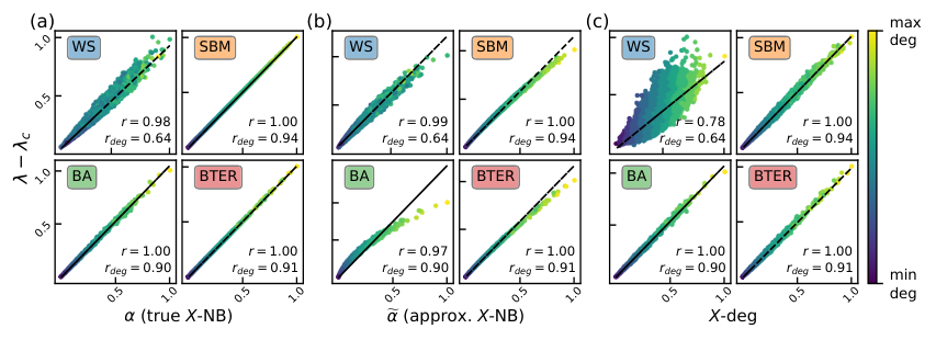
In Fig. 4a we measure how correlated the true value of -NB, denoted by , is to the true eigen-drop. For SBM, BA, and BTER graphs, the magnitude of lines up extremely closely with the value of the eigen-drop, showing a correlation coefficient of . In all cases, is better correlated to the eigen-drop than degree (as shown by the correlation coefficients ). In WS we see considerably more variance than in other ensembles though is still an excellent predictor of the eigen-drop, at . This picture repeats itself when using the approximate value of -NB, (Fig. 4b), and -degree (Fig. 4c). seems to slightly underestimate the eigen-drop, while -degree has noticeably more variance than the other two statistics, especially in WS. All three statistics are better correlated to the eigen-drop than degree in all graph ensembles. We highlight that even when some of the panels in Fig. 4 are not precisely linear, they all show that the eigen-drop is an increasing function of all of , , and -degree. These results encourage us to use -NB and -degree as immunization strategies. Further, using has very little advantage over , and therefore we are justified in using Algorithm 2 instead Algorithm 1 for computational reasons.
6.3 Immunization with X-NB and X-degree
How effective are -NB and -degree at immunization? We remove and percent of nodes using different strategies and evaluate the resulting eigenvalue. We use the immunization strategies node degree (degree), -core index (core), NetShield (NS), Collective Influence (CI), NB-centrality (NB), approximate -NB (XNB), and -degree (Xdeg). For computational reasons, we do not use the true value of -NB; for more details on baselines see Section C.1. In all data sets, core had the least performance and is therefore not shown in our results. We hypothesize this is because many nodes can have the same -core index at the same time, so core cannot identify which is the best one among all of them.
| degree | NS | CI | Xdeg | NB | XNB | |
|---|---|---|---|---|---|---|
| 1% | 62.76 | 61.44 | 62.88 | 62.90 | 62.92 | 62.91 |
| BA 2% | 68.84 | 66.94 | 68.97 | 68.99 | 69.01 | 69.01 |
| 3% | 72.42 | 70.09 | 72.56 | 72.57 | 72.59 | 72.59 |
| 1% | 6.28 | 6.40 | 6.41 | 6.45 | 6.46 | 6.46 |
| BTER 2% | 10.60 | 10.72 | 10.80 | 10.85 | 10.86 | 10.86 |
| 3% | 14.31 | 14.40 | 14.55 | 14.61 | 14.63 | 14.63 |
| 1% | 3.31 | 3.41 | 3.40 | 3.43 | 3.44 | 3.44 |
| SBM 2% | 6.00 | 6.16 | 6.19 | 6.23 | 6.25 | 6.25 |
| 3% | 8.52 | 8.66 | 8.76 | 8.80 | 8.82 | 8.82 |
| 1% | 1.41 | 1.17 | 1.50 | 1.52 | 1.63 | 1.63 |
| WS 2% | 2.52 | 2.09 | 2.97 | 2.98 | 3.11 | 3.11 |
| 3% | 3.66 | 2.94 | 4.41 | 4.41 | 4.57 | 4.58 |
| degree | CI | Xdeg | degree | CI | Xdeg | degree | CI | Xdeg | |
|---|---|---|---|---|---|---|---|---|---|
| AS-1 | 0.74 | 0.74 | 2.35 | 6.70 | 13.51 | 15.43 | 71.65 | 78.26 | 75.92 |
| AS-2 | 2.02 | 2.02 | 4.00 | 17.09 | 22.36 | 28.17 | 87.60 | 89.61 | 87.02 |
| Social-Slashdot | 0.95 | 1.02 | 1.02 | 4.63 | 6.06 | 6.94 | 23.65 | 28.11 | 30.30 |
| Social-Twitter | 2.18 | 2.18 | 1.98 | 13.21 | 13.97 | 13.68 | 41.10 | 42.88 | 43.39 |
| Transport-California | 0.00 | 0.00 | 0.65 | 2.65 | 0.65 | 2.65 | 5.09 | 5.09 | 7.80 |
| Transport-Sydney | 0.00 | 0.00 | 0.00 | 0.00 | 0.00 | 6.50 | 0.00 | 7.37 | 9.49 |
| Web-NotreDame | 9.34 | 9.34 | 9.34 | 12.10 | 13.79 | 13.79 | 14.37 | 14.37 | 19.22 |
Table 1 shows the percentage reduction of the eigenvalue after immunization, averaged over repetitions on synthetic graphs. We can arrange immunization strategies in tiers according to increasing performance: strategies within a tier have comparable performance across data sets. The third tier is made up of NS and degree. They perform similarly because NS targets the largest eigenvalue of the adjacency matrix, which is largely dominated by node degree. Strategies in this tier perform substantially better than core (not shown), and are very close to the strategies in the next two tiers, i.e. degree is a very strong baseline in this task. The second tier is comprised of CI and Xdeg, with Xdeg having a slight advantage over CI. Finally, the best performance was achieved by NB and XNB. Their performances were almost indistinguishable in most data sets, though they have a small margin over CI and Xdeg.
Strategies in the best two tiers, i.e. CI, Xdeg, NB and XNB, all showed standard deviations of similar magnitude across all data sets (not shown), and the ordering in increasing performance CI ¡ Xdeg ¡ NB XNB is statistically significant at (see Appendix C.5). Further, the best two (NB and XNB) use the principal NB-eigenvector, whereas CI and Xdeg depend only on node degree, and are therefore much more computationally efficient.
Table 2 shows the results on real data sets, where we have run only degree, CI, and Xdeg for computational reasons. We use social networks [32, 33], transportation networks, [34, 35, 33], Autonomous Systems (AS) of the Internet networks [36, 12], and web crawl networks [37]. See Section C.2 for data set descriptions. We remove from each network , , and nodes at a time. Again, degree is a very strong baseline, but it is never better than both CI and Xdeg at the same time. All three strategies are able to drastically immunize the autonomous systems networks AS-1 and AS-2 at nodes removed, probably owing to the fact that their degree distribution is extremely heterogeneous and thus the nodes with largest degree have a large eigen-drop. In all other networks, -degree achieves the best performance. An interesting case is that of Transport-Sydney. The node identified by all three strategies has an eigen-drop of exactly . Following Corollary 1, this means that the chosen node lies outside of the -core of the graph and thus has no impact on non-zero NB-eigenvalues. After nodes are removed, both degree and CI continue to achieve zero eigen-drop, while Xdeg already identifies the correct nodes and ahieves decrease. Even at nodes removed, degree cannot identify nodes that generate an eigen-drop. A similar case occurs on Transport-California, where the first node identified by degree and CI generates no eigen-drop, while Xdeg is able to correctly identify influential nodes.
We conclude that in cases where efficiency is of the essence, Xdeg is the best overall immunization strategy, as it has a slight advantage over CI and its performance is close to optimal. If effectiveness is more important than efficiency, either XNB or NB should be used.
7 Conclusion
We developed a theory of spectral analysis for the NB-matrix by studying what happens to its largest eigenvalue when one node is removed from the network. Our theory is independent of the structure of the graph, i.e. we make no assumptions of locally tree-like structure or density or length of cycles, as is usual in other studies. We find two new node-level statistics, or centrality measures, -NB centrality and -degree, which are excellent predictors of a node’s influence on the largest NB-eigenvalue. Finally, we focus on the application of targeted immunization, where we propose two new algorithms that are shown to be more effective than other strategies for a variety of real and synthetic graph ensembles.
Our techniques open many possibilities for further research. For instance, the left-hand side of Equation (12) is reminiscent to certain quantities used in the theory of eigenvalue interlacing [38], while the matrix on the right-hand side is known as the resolvent of , which has many applications in random matrix theory [39]. On a different note, Cvetkovic et al. 1980 highlight that most matrices associated to graphs are linear combinations of , , and , whereas the NB-matrix is associated with a quadratic combination of , , and , via Equation (3). In the future, we will explore which other matrices associated with graphs can be studied via quadratic, or higher order, combinations of , , and .
We focused on the application to targeted immunization. However, other applications of NB-eigenvalues exist – e.g., community detection and graph distance. Further studying the behavior of NB-eigenvalues under small perturbations of the graph, using the framework presented here, has potential to affect those applications.
Acknowledgements
L.T. thanks Gabor Lippner for many invaluable discussions.
References
- Alon et al. [2007] Noga Alon, Itai Benjamini, Eyal Lubetzky, and Sasha Sodin. Non-backtracking random walks mix faster. Commun. Contemp. Math., 9(4):585–603, 2007.
- Torres et al. [2019] Leo Torres, Pablo Suárez-Serrato, and Tina Eliassi-Rad. Non-backtracking cycles: length spectrum theory and graph mining applications. Applied Network Science, 4(1), 2019.
- Bordenave et al. [2015] Charles Bordenave, Marc Lelarge, and Laurent Massoulié. Non-backtracking spectrum of random graphs: Community detection and non-regular ramanujan graphs. In FOCS, pages 1347–1357, 2015.
- Krzakala et al. [2013] Florent Krzakala, Cristopher Moore, Elchanan Mossel, Joe Neeman, Allan Sly, Lenka Zdeborová, and Pan Zhang. Spectral redemption in clustering sparse networks. Proc. Natl. Acad. Sci. USA, 110(52):20935–20940, 2013. ISSN 0027-8424.
- Morone et al. [2016] Flaviano Morone, Byungjoon Min, Lin Bo, Romain Mari, and Hernán A Makse. Collective influence algorithm to find influencers via optimal percolation in massively large social media. Scientific Reports, 6:30062, 2016.
- Morone and Makse [2015] Flaviano Morone and Hernán A Makse. Influence maximization in complex networks through optimal percolation. Nature, 524(7563):65, 2015.
- Mellor and Grusovin [2019] Andrew Mellor and Angelica Grusovin. Graph comparison via the nonbacktracking spectrum. Phys. Rev. E, 99(052309), 2019.
- Martin et al. [2014] Travis Martin, Xiao Zhang, and M. E. J. Newman. Localization and centrality in networks. Phys. Rev. E, 90(052808), 2014.
- Arrigo et al. [2018a] Francesca Arrigo, Peter Grindrod, Desmond J. Higham, and Vanni Noferini. Non-backtracking walk centrality for directed networks. J. Complex Networks, 6(1):54–78, 2018a.
- Kempton [2016] Mark Kempton. Non-backtracking random walks and a weighted ihara’s theorem. Open Journal of Discrete Mathematics, 6:207–226, 2016.
- Arrigo et al. [2018b] Francesca Arrigo, Peter Grindrod, Desmond J. Higham, and Vanni Noferini. On the exponential generating function for non-backtracking walks. Linear Algebra and its Applications, 556:381 – 399, 2018b.
- Karrer et al. [2014] Brian Karrer, Mark EJ Newman, and Lenka Zdeborová. Percolation on sparse networks. Phys. Rev. Lett., 113(208702), 2014.
- Hamilton and Pryadko [2014] Kathleen E Hamilton and Leonid P Pryadko. Tight lower bound for percolation threshold on an infinite graph. Phys. Rev. Lett., 113(208701), 2014.
- Pastor-Satorras et al. [2015] Romualdo Pastor-Satorras, Claudio Castellano, Piet Van Mieghem, and Alessandro Vespignani. Epidemic processes in complex networks. Rev. Mod. Phys., 87(3), 2015.
- Newman [2002] Mark EJ Newman. Spread of epidemic disease on networks. Phys. Rev. E, 66(016128), 2002.
- Shrestha et al. [2015] Munik Shrestha, Samuel V Scarpino, and Cristopher Moore. Message-passing approach for recurrent-state epidemic models on networks. Phys. Rev. E, 92(022821), 2015.
- Castellano and Pastor-Satorras [2018] Claudio Castellano and Romualdo Pastor-Satorras. Relevance of backtracking paths in recurrent-state epidemic spreading on networks. Phys. Rev. E, 98(052313), 2018.
- Radicchi and Castellano [2016] Filippo Radicchi and Claudio Castellano. Leveraging percolation theory to single out influential spreaders in networks. Phys. Rev. E, 93(062314), 2016.
- Chen et al. [2016] Chen Chen, Hanghang Tong, B. Aditya Prakash, Charalampos E. Tsourakakis, Tina Eliassi-Rad, Christos Faloutsos, and Duen Horng Chau. Node immunization on large graphs: Theory and algorithms. TKDE, 28(1):113–126, 2016.
- Zhang [2015] Pan Zhang. Nonbacktracking operator for the ising model and its applications in systems with multiple states. Phys. Rev. E, 91(042120), 2015.
- Coste and Zhu [2019] Simon Coste and Yizhe Zhu. Eigenvalues of the non-backtracking operator detached from the bulk. CoRR, abs/1907.05603, 2019.
- Arrigo et al. [2019] Francesca Arrigo, Desmond J. Higham, and Vanni Noferini. Non-backtracking pagerank. J. Sci. Comput., 80(3):1419–1437, 2019.
- Kitsak et al. [2010] Maksim Kitsak, Lazaros K Gallos, Shlomo Havlin, Fredrik Liljeros, Lev Muchnik, H Eugene Stanley, and Hernán A Makse. Identification of influential spreaders in complex networks. Nature Physics, 6(11):888, 2010.
- Poux-Médard et al. [2019] Gaël Poux-Médard, Romualdo Pastor-Satorras, and Claudio Castellano. Influential spreaders for recurrent epidemics on networks. CoRR, abs/1912.08459, 2019.
- Everett and Borgatti [2010] Martin G. Everett and Stephen P. Borgatti. Induced, endogenous and exogenous centrality. Social Networks, 32(4):339–344, 2010.
- Lin et al. [2017] Yuan Lin, Wei Chen, and Zhongzhi Zhang. Assessing percolation threshold based on high-order non-backtracking matrices. In WWW, pages 223–232, 2017.
- Watts and Strogatz [1998] Duncan J Watts and Steven H Strogatz. Collective dynamics of ‘small-world’networks. Nature, 393(6684):440, 1998.
- Girvan and Newman [2002] Michelle Girvan and Mark EJ Newman. Community structure in social and biological networks. Proc. Natl. Acad. Sci. USA, 99(12):7821–7826, 2002.
- Karrer and Newman [2011] Brian Karrer and Mark EJ Newman. Stochastic blockmodels and community structure in networks. Phys. Rev. E, 83(016107), 2011.
- Albert and Barabási [2002] Réka Albert and Albert-László Barabási. Statistical mechanics of complex networks. Reviews of Modern Physics, 74(1):47, 2002.
- Seshadhri et al. [2012] Comandur Seshadhri, Tamara G Kolda, and Ali Pinar. Community structure and scale-free collections of erdős-rényi graphs. Phys. Rev. E, 85(056109), 2012.
- De Domenico et al. [2013] Manlio De Domenico, Antonio Lima, Paul Mougel, and Mirco Musolesi. The anatomy of a scientific rumor. Scientific Reports, 3:2980, 2013.
- Leskovec et al. [2009] Jure Leskovec, Kevin J. Lang, Anirban Dasgupta, and Michael W. Mahoney. Community structure in large networks: Natural cluster sizes and the absence of large well-defined clusters. Internet Mathematics, 6(1):29–123, 2009.
- Opsahl [2011] Tore Opsahl. Why anchorage is not (that) important: Binary ties and sample selection, 2011. URL toreopsahl.com/datasets/#usairports.
- for Research Core Team [2013] Transportation Networks for Research Core Team. Transportation networks for research, 2013. URL github.com/bstabler/TransportationNetworks/.
- Zhang et al. [2004] Beichuan Zhang, Raymond A. Liu, Daniel Massey, and Lixia Zhang. Collecting the internet as-level topology. Computer Communication Review, 35(1):53–61, 2004.
- Albert et al. [1999] Réka Albert, Hawoong Jeong, and Albert-László Barabási. Diameter of the world-wide web. Nature, 401(6749):130–131, 1999.
- Godsil and Royle [2013] Chris Godsil and Gordon F Royle. Algebraic graph theory, volume 207. Springer Science & Business Media, 2013.
- Tao [2010] Terrence Tao. The semi-circular law, 2010. URL terrytao.wordpress.com/2010/02/02/254a-notes-4-the-semi-circular-law.
- Cvetkovic et al. [1980] Dragoš M Cvetkovic, Michael Doob, Horst Sachs, et al. Spectra of graphs, volume 10. Academic Press, New York, 1980.
- Barabási [2016] Albert-László Barabási. Network science. Cambridge University Press, 2016.
- Kolda et al. [2014] Tamara G. Kolda, Ali Pinar, Todd D. Plantenga, and C. Seshadhri. A scalable generative graph model with community structure. SIAM J. Sci. Comput., 36(5), 2014.
- Hagberg et al. [2008] Aric Hagberg, Pieter Swart, and Daniel S Chult. Exploring network structure, dynamics, and function using networkx. Technical report, Los Alamos National Lab.(LANL), Los Alamos, NM (United States), 2008.
Appendix A Technical Lemmas
In this subsection, is the NB-matrix of a graph , is defined in Section 2, and are the Perron eigenvalue and corresponding unit right eigenvector of . Let also as in Equation (2) and let .
Lemma A.1.
is a left eigenvector of corresponding to .
Proof.
Since is symmetric and , we have . Now implies , which completes the proof. ∎
Lemma A.2.
Suppose is such that . Let be the left unit eigenvector of corresponding to . Then, we have , where
| (28) |
Proof.
Remark 4.
Both and determine the same node centrality ranking, though the latter is easier to compute. However, the normalization is fundamental in our theory, which makes the more appropriate choice. Lemma A.2 allows us to compute only with the knowledge of and , which is much more efficient than computing and directly.
Appendix B Complexity Analysis of Algorithm 3
In Section 4.2 we used a standard map (i.e. hash table, or dictionary) to store the -degree values in line of Algorithm 3. Alternatively, we can use an indexed priority queue (IPQ). An IPQ is a data structure that behaves like a priority queue except that, additionally, elements in the IPQ can be updated efficiently. The underlying data structure is a max-heap. An IPQ can find the maximum element in the heap, as well as update any element, in logarithmic time.
In this case, line of Algorithm 3 takes operations to compute the -degree values plus operations to heapify the IPQ. Further, lines and take time, which yields a time complexity of
| (31) |
B.1 Homogeneous degree distribution
In networks with a homogeneous degree distribution (e.g. Poisson) we can estimate and , where is the average degree. This yields total complexity for the IPQ version, while the map version gives . If and , the IPQ version scales better in the worst case scenario.
B.2 Heterogeneous degree distribution
In networks whose degree distribution is well approximated by a power law, the probability of finding a node of degree scales as , for some . In this case, the first few nodes removed by Algorithm 3 will usually have large degree, comparable to the largest degree in the network, for each . Further, in the worst case scenario, each of their neighbors will also have a degree comparable to and thus for each . Using [41] yields for the map version and for the IPQ version. In the typical case , the exponent varies between and .
B.3 Average runtime
We have provided the analysis of worst case scenario runtime. However, the average runtime of both the IPQ and map versions is close to linear, as shown in Figure 2. This figure was generated by first sampling a degree sequence from a power-law density , and then generating a graph at random using the configuration model. Self-loops and multi-edges were removed and only the largest component was kept. Each marker is the average of repetitions. We used .
| nodes | edges | |||||
|---|---|---|---|---|---|---|
| AS-1 [36] | AS | digital communication | 34,761 | 107,720 | 151.442 | 2,760 |
| AS-2 [12] | AS | digital communication | 22,963 | 48,436 | 64.678 | 2,390 |
| Social-Slashdot [33] | users | friendships | 77,360 | 469,180 | 128.550 | 2,539 |
| Social-Twitter [32] | users | friendships | 456,290 | 12,508,221 | 636.147 | 51,386 |
| Transport-California [35] | intersections | roads | 1,957,027 | 2,760,388 | 3.321 | 12 |
| Transport-Sydney [35] | intersections | roads | 32,956 | 38,787 | 2.266 | 10 |
| Web-NotreDame [37] | websites | hyperlinks | 325,729 | 1,090,108 | 175.657 | 10,721 |
Appendix C Experimental Setup
C.1 Base lines
Degree.
The degree of a node , denoted is the number of neighbors it has in the graph. Nodes of degree have zero Collective Influence, -degree, NB-centrality, -NB centrality.
-core index.
The -core index of a node, also called coreness, is defined as follows. First, iteratively remove all nodes of degree until there are none. All nodes removed in this step are assigned a value of -core index of . Then, iteratively remove all nodes of degree ; all nodes removed at this step have -core . Repeat this process until there are no more nodes in the graph. Notably, following Corollary 1, all nodes with -core value of have zero NB-centrality.
NB-centrality.
NetShield.
NetShield is an efficient algorithm that identifies a subset of nodes with the highest “shield-value”, which is defined as the impact a node, or set of nodes, has on the largest eigenvalue of the adjacency matrix [19].
Collective Influence.
The Collective Influence (CI) of node is
| (32) |
though this definition can be generalized to include nodes in arbitrarily large neighborhoods around [6]. Note that this is quite similar in nature to -degree in Equation (24). We think of -degree as a second-order aggregation of the values of the neighbors of , while CI is a first-order aggregation. Further, one can apply Algorithm 3 to perform targeted immunization based on CI instead of -degree, and hence they have the same running time complexity (see Section 4.2 and Appendix B). Morone et al. 2016 claim that the CI algorithm runs in time, though we were not able to reproduce this result. In any case, any efficient algorithm that computes CI can be used to compute -degree as well.
C.2 Data sets
All synthetic graphs have nodes and parameters were chosen so that the average degree was approximately . SBM graphs were generated with two blocks, or communities, so that the average within-block degree is and the between-block degree is . WS graphs generated with rewiring probability . BTER graphs were generated with target average local clustering coefficient of , and target global clustering coefficient of . BTER graphs were generated with the authors’ implementation [42]; all other graphs were generated using NetworkX [43] version 2.3. After generation, we extracted the largest connected component of each graph and converted all multi-edges to single edges and deleted self-loops. graphs were generated from each ensemble. Table 3 describes the real data sets used. Directed networks were converted to undirected, and only the largest connected component of each data set was used.
C.3 Approximating the Largest Eigenvalue
Since nodes of large degree are bound to induce a larger eigen-drop than those of small degree, we chose target nodes at random by sampling of nodes from each graph, proportionally to their degree. This was achieved by sampling one edge at random, with replacement, and then choosing one of its endpoints randomly. This yields a probability of sampling node equal to .
C.4 Predicting the Eigen-drop
Nodes were sampled in the same way as in C.3. Figure 4 shows correlation coefficients, defined as the covariance divided by the product of the standard deviations of the two variables. We computed the correlation between the eigen-drop and each of the statistics: , , -degree, and degree. No three-way correlation was computed.
C.5 Immunization with X-NB and X-degree
To confirm the ordering in increasing performance CI Xdeg NB XNB, we used a one-sided Wilcoxon signed-rank test, which is a non-parametric version of the paired T-test. In a paired sample setting, this test tests the null hypothesis that the median of the differences between the two samples is positive, against the alternative that it is negative. Therefore, a small -value means that there is little probability that the first sample’s median is smaller than the second’s. For each graph ensemble and each percentage of removed nodes (1%, 2%, 3%), the ranking CI Xdeg NB was confirmed with in all cases. Further, we have NB XNB in WS networks () and BTER networks (), and NB XNB in BA networks () and SBM networks (). We summarize these results by writing CI Xdeg NB XNB.