Photon-mediated Peierls Transition of a 1D Gas in a Multimode Optical Cavity
Abstract
The Peierls instability toward a charge density wave is a canonical example of phonon-driven strongly correlated physics and is intimately related to topological quantum matter and exotic superconductivity. We propose a method to realize an analogous photon-mediated Peierls transition, using a system of one-dimensional tubes of interacting Bose or Fermi atoms trapped inside a multimode confocal cavity. Pumping the cavity transversely engineers a cavity-mediated metal–to–insulator transition in the atomic system. For strongly interacting bosons in the Tonks-Girardeau limit, this transition can be understood (through fermionization) as being the Peierls instability. We extend the calculation to finite values of the interaction strength and derive analytic expressions for both the cavity field and mass gap. They display nontrivial power law dependence on the dimensionless matter-light coupling.
Introduction — The interaction between electrons and phonons has traditionally played a leading role in the formation of quantum phases of matter, with superconductivity being a prime example. Quantum simulation in optical lattices provides an enticing platform to explore new phases Bloch et al. 2008, but phonon-driven physics lies beyond traditional optical lattice capabilities as they are externally imposed and rigid. The use of high-finesse optical cavities has been suggested as a route to overcome this by making the optical lattice fully dynamical and compliant Lewenstein et al. 2006; Gopalakrishnan et al. 2009; Gopalakrishnan et al. 2010. This requires cavities that support multiple degenerate modes, as single-mode cavities only allow dynamics of the lattice intensity, not its period. That is, while single-mode cavities have provided access to a diverse array of exotic quantum phenomena including self-organization Domokos and Ritsch 2002, supersolids Leonard et al. 2017, spinor density-wave polariton condensates Kroeze et al. 2018, dynamical Mott insulators Klinder et al. 2015; Landig et al. 2016, and dynamical spin-orbit coupling Kroeze et al. 2019, only multimode cavities support fully emergent optical lattices whose amplitude and periodicity may vary Lewenstein et al. 2006; Gopalakrishnan et al. 2009; Gopalakrishnan et al. 2010. Multimode cavity experiments have already engineered a variety of photon-mediated interatomic interactions Kollár et al. 2014; Vaidya et al. 2018; Guo et al. 2019a; Guo et al. 2019b. These could lead to the creation of new many-body systems and states of matter such as quantum liquid crystals made of photons and superfluid atoms Gopalakrishnan et al. 2009; Gopalakrishnan et al. 2010 and superfluids exhibiting Meissner-like effects Ballantine et al. 2017.
As we will show below, confocal multimode cavities coupled to one dimensional (1D) quantum gases provide a way to realize controllable electron-phonon-like interactions using ultracold atoms. Other proposals to study this physics include coupling fermionic atoms to an optical waveguide Fraser and Piazza 2019, or to a crystal of trapped ions Bissbort et al. 2013. One-dimensional ultracold gases also allow one to explore pairing physics with bosons, as resonant atomic collisions provide a knob to make bosons strongly repel Chin et al. 2010; Haller et al. 2010, even to the point that they behave like fermions Paredes et al. 2004; Kinoshita et al. 2004; Haller et al. 2009. For such systems, the addition of attractive interactions can cause dramatic effects. Indeed, for 1D systems, even weakly attractive interactions result in instabilities leading to strong correlations such that the quasiparticle picture breaks down and collective modes emerge Giamarchi 2003; Gogolin et al. 2004; Tsvelik 2003. A paradigmatic example is the Peierls instability that occurs because the susceptibility of a free Fermi gas diverges due to infinitesimal density perturbations at twice the Fermi wavevector Peierls 1996. If free phonons exist, then it is possible for the system to create an emergent lattice that matches this wavevector. Due to the diverging susceptibility, the system undergoes a metal-insulator transition and dynamically generates a mass gap. The Peierls transition is a canonical example of phonon-driven physics and intimately related to the continuum Su-Schrieffer-Heeger (SSH) model of 1D topological insulators in 1D Su et al. 1979. Numerical work has shown the analogue of a Peierls transition for atoms in an optical lattice, where intersite hopping of bosonic atoms is modulated by the spin state of a second species of atoms González-Cuadra et al. 2018.
In this Letter, we show that a Peierls instability occurs in a strong, repulsively interacting 1D bosonic gas trapped inside a transversely pumped confocal multimode optical cavity. Building on demonstrated experimental capabilities Vaidya et al. 2018; Guo et al. 2019a, we predict that by tuning the interatomic interactions to the hard-core, Tonks-Girardeau (TG) limit Tonks 1936; Girardeau 1960, the cavity can mediate a Peierls transition in the bosonic gas, with a mass gap and photon amplitude that is exponential in the matter-light coupling. By using bosonization, we then extend these calculations to finite values of the interatomic interaction, as well as to interacting fermionic systems. In agreement with Ref. González-Cuadra et al. 2018, we show that in these cases, the cavity can mediate a metal-insulator transition, albeit one of different character. Moreover, we show that the dynamically generated mass gap and photon amplitude have a nontrivial power law dependence on the matter-light coupling. Self-organization of fermions in a single-mode cavity has also been previously discussed theoretically Keeling et al. 2014; Piazza and Strack 2014; Chen et al. 2014, but here the diverging susceptibility requires the single cavity mode and Fermi wavevectors to match. Experimentally realizing a photon-mediated Peierls transition would open new avenues toward exploring the role of Fermi surface nesting and charge density waves in exotic superconductors in simulators operating in a quantum-optical, many-body context.

Model — The system considered, depicted in Fig. 1, consists of 1D tubes of atoms placed in a transversely pumped confocal optical cavity. As already noted, multiple optical modes are needed to allow a fully emergent optical lattice. For true multimode operation, these modes must be degenerate or near degenerate. A confocal cavity is the simplest stable resonator allowing such degeneracy Siegman 1986. To achieve a 1D trap geometry and uniform atom-cavity coupling, we confine bosonic atoms in a strong -periodic 2D optical lattice formed by a retroreflected beam along the pump direction and an intracavity standing wave along the cavity axis. A pump field along has a wavevector close to a cavity resonance. By choosing the tube–lattice period such that is an integer, the tubes lie at the peaks of the pump and cavity standing-wave fields so the atoms coherently Bragg scatter light into the cavity. As a result, in contrast to experiments on self-organization Baumann et al. 2010, there is no spontaneous atomic organization in the plane; rather, the atoms superradiantly emit into the cavity regardless of pump strength. We choose the tubes to be near the cavity midplane , and the long Rayleigh range of a confocal cavity ensures that the tubes at different will behave identically. In , we choose all tubes to be centered at the same since tubes at different decouple, as discussed in the Supplemental Material Sup. As such, we will describe the atoms in tube through a bosonic field , varying only along the free direction. Degenerate confocal cavities with BECs in optical traps are practicable with existing technology Guo et al. 2019b.
We can write the Hamiltonian of the system as follows Sup:
| (1) |
The first term, , describes the cavity photons, where is measured with respect to the transverse pump frequency. We sum only over cavity modes that are near resonant with the pump. Modes are labeled by the longitudinal index and transverse index . The second and third terms describe atoms with mass , chemical potential , and a contact interaction of strength . We sum over an array of tubes, labeled by , positioned in an array along . The last term describes the coupling of the atomic density to the cavity photons, as induced by the pump. This term describes how the atomic density scatters photons between the transverse pump and the cavity modes. As described in Ref. Sup, this term can be derived by adiabatically eliminating excited states of the atoms, yielding an effective AC light shift. The photon field is written as a sum over cavity modes . The transverse mode functions are found by taking the eigenmodes of the cavity—Gauss–Hermite functions of order in the and directions, respectively—and convolving these with the Gaussian tube profile in the direction; see Ref. Sup. The factors come from the longitudinal spatial mode profile evaluated at the atom positions, and are discussed below. As noted above, this final term is a source for cavity photons independent of the density profile —the tube spacing causes atoms to coherently scatter the pump into the cavity with intensity Kirton et al. 2019. The prefactor is the effective matter-light coupling where is the bare coupling, the pump Rabi frequency, and is the pump-atom detuning.
As the Gauss–Hermite functions form a complete basis set, one might expect that could take any spatial profile. This would allow the cavity light to match the atomic density, inducing a local interaction. There are complications, however. First, while transverse modes become degenerate at confocal resonances of the cavity, they do so in alternating odd and even families, set by the parity of . We assume even hereon. Secondly, the factors modify the sum over modes. As shown in Ref. Guo et al. 2019a, the longitudinal mode profile assumes a form , where depends on which family we consider. This includes the effects of the Gouy phase Siegman 1986, leading to an dependence. If we consider the special case where is a multiple of , we then see that for successive, even , the factor is sequentially . The missing Gauss–Hermite functions prevent from obtaining an arbitrary form; equivalently, this yields a nonlocal photon-mediated interaction. This can be nulled by using two pumps resonant with families and , yielding a local interaction Guo et al. 2019a.
Both the matter-light coupling and interatomic interaction strength are experimentally tunable parameters Bloch et al. 2008. In particular, the system may be tuned into the TG regime, i.e., , using tight trapping and collisional resonances, where is the average 1D density Kinoshita et al. 2004; Paredes et al. 2004. The atoms behave like free fermions in this limit Tonks 1936; Girardeau 1960 and so will exhibit a Peierls instability. Even strongly repulsive bosons away from the TG limit exhibit this instability.
Steady state — We investigate the Peierls instability using a mean-field description of the photon field. We therefore consider the equations of motion for the expectation of photon operators:
| (2) |
where we have included a term accounting for cavity losses. Assuming a steady state, the mean field is
| (3) |
For simplicity, we consider the perfectly degenerate limit . Pumping two families as discussed above, , allowing for the explicit evaluation of the sum over modes: 11 1 See Ref. Guo et al. 2019a for near-degenerate case where the interaction becomes finite in range; Peierls physics remains the same as long as the interaction range is less than the intertube spacing.. Here, is the transverse width of an individual tube, is the beam waist, and we made a simplifying assumption that the tubes are in the upper half of the cavity, , to avoid mirror-image interactions Vaidya et al. 2018. As all tubes behave identically, we can insert this into Eq. (3) to give:
| (4) |
where we have defined the dimensionless matter-light coupling and is the Fermi velocity in the TG limit. Later, it will be convenient to parameterize this as and also introduce the quantity . The atoms will coherently scatter light into the cavity, so any nonzero density of atoms implies . We will find that becomes nonzero at the Peierls transition, leading to the dynamical generation of a mass gap.
Adiabatic elimination of photons from our model at the mean-field level leads to completely conservative dynamics—this is a generic feature of a Rabi-like matter-light coupling Damanet et al. 2019. The resulting conservative dynamics is determined entirely by an effective Hamiltonian, , and so the steady-state condition becomes equivalent to minimizing this with respect to the mean field . The atomic and atom-cavity coupling parts of come from substituting Eq. (4) into Eq. (1) (considering a single tube), while the cavity part can be written as . We consider only constant values of and , in which case can be absorbed into a redefinition of the chemical potential, . Henceforth we shall deal only with .
Low energy & Bosonization — The atomic system can be described using bosonization, which provides us with a description of our system in terms of two new bosonic fields, and its canonical conjugate Coleman 1975; Haldane 1981; Giamarchi 2003; Gogolin et al. 2004. The former is related to the atomic density via , while the latter is related to the current in the system Haldane 1981. In terms of these, the steady-state condition Eq. (4) reduces to . As such, the effective mean-field Hamiltonian discussed above can be written in terms of the bosonized fields as:
| (5) |
The first line describes the atomic and cavity systems, using the standard result for bosonization of the atoms. The atomic interactions are encoded via the parameter which depends on in a complicated fashion Cazalilla 2004. For large repulsive interactions, this relationship can be approximated by , with the TG limit achieved at , while corresponds to free bosons Cazalilla 2004. The second line describes the relevant part of the matter-light coupling and will generate a gap. We have allowed for the possibility that the matter-light coupling and photon field might carry opposite signs, and we keep only terms which are most relevant in a renormalization group sense, which restricts our analysis to values .
While in the present work our primary system of interest is bosons with short-range, repulsive interactions, bosonization allows one to also describe the low-energy physics of bosons with long-range interactions or interacting fermions Giamarchi 2003; Gogolin et al. 2004; Cazalilla et al. 2011. Such systems are described by a Luttinger parameter , and so in the following, we allow for arbitrary values of . Results for are applicable to bosons with short-ranged interactions or fermions with attractive interactions, whereas corresponds to 1D repulsive fermions or bosonic systems with long-range interactions, the latter of which has been realized in Refs. Tang et al. 2018; Kao et al. 2020.
Tonks-Girardeau limit — The atoms behave as free fermions in the TG limit Tonks 1936; Girardeau 1960. This is evident in our low-energy description at where it is possible to express the bosonic operators as a pair of chiral fermions. In terms of these, the low-energy Hamiltonian Eq. (5) becomes the 1D Dirac Hamiltonian with a mass Luther and Emery 1974; Sup that is subject to the steady state condition. This system is the same as the SSH model Su et al. 1979 whose solution is well known. Carrying it over to the present case, we find that , where is the Fermi energy. The self-consistent photon field is therefore given by
| (6) |
The atomic system is insulating with a mass gap of . The applicability of the low-energy description relies on being the largest scale in the system. In particular, we require that , which in turn requires .
Finite interaction — The system is quite different for . It is strongly correlated and interacting, but can no longer be mapped to the SSH model. Nevertheless, an exact solution for the steady state can be found, although the cases of positive and negative need to be treated separately; we will find below that these correspond to and , respectively. For , the atomic part of the Hamiltonian is that of the Sine-Gordon or massive Thirring model with a positive mass term Coleman 1975; Giamarchi 2003; Gogolin et al. 2004. This is an exactly solvable field theory and many of its properties are well known Bergknoff and Thacker 1979; Zamolodchikov and Zamolodchikov 1979. In particular, the mass gap of the model becomes renormalized due to the interactions, , with a -dependent constant provided in Ref. Sup. Using this, we derive the following steady-state condition from which to determine ,
| (7) |
This has a solution only for . Rearranging, we find that the self-consistent photon field and mass gap are
| (8) | |||||
| (9) |
where is given in Ref. Sup. The amplitude of the photon field now has a power law rather than the exponential dependence on in the TG limit. Furthermore, the exponent differs from that appearing in the mass gap. The TG limit cannot be recovered from the above expression and must be treated separately as in the previous section. This highlights the strong correlations in the interacting system. The photon field oscillates at wavevector , which is times .
The model maps to the massive Thirring model for , but with a negative mass parameter. As explained in Ref. Sup, this change in sign of the mass term results in the spectrum of the model being inverted; i.e., the ground state becomes the highest excited state Sup. Spectral inversion also occurs when changing the sign of the interactions—i.e., taking . Combining these, we find that for and , the renormalized mass gap and self-consistent photon field are
| (10) | ||||
| (11) |
where are related to by .
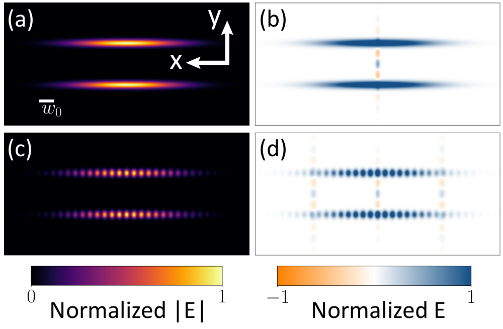
Experimental signatures — One may image the atomic density profile by using the spatial resolving power of the degenerate cavity. This provides a direct signature of the Peierls instability as a density wave. Figure 2 shows this, calculated using results from Ref. Guo et al. 2019a. The spatial modulation of the light amplitude from the atomic image is a signature of the Peierls transition; a mirror image appears at . The geometry of the confocal cavity conveniently provides both the emission of the atomic density image (long thin tubes) and its Fourier transform (vertical stripes) Guo et al. 2019a. Thus, a density modulation of wavevector results in Bragg peaks manifest as vertical stripes. These are positioned at . (Each stripe is the Fourier transform of the -displaced atom image.)
The power-law scaling between the oscillation amplitude of the detected light and the parameter depends critically on the atom interactions; see Eq. (8). The Luttinger parameter can thus be experimentally measured through the dependence of this exponent on . This can be tuned through its dependence on the pump intensity or by the cavity-pump detuning .
Probing the system by stimulating a particular photon mode realizes cavity-enhanced Bragg spectroscopy Mottl et al. 2012. In a degenerate cavity, the probe field profile can be tailored with holographic beam shaping to have a particular wavevector. Thus, dynamic susceptibility can be measured as a function of and excitation energy by also tuning the detuning between the probe and pump. The response of the system manifests as an increase in photon population, allowing the gap to be measured.
In conclusion, we have shown that multimode confocal cavities can be used to realize the Peierls transition for both Bose and Fermi gases. Away from the simple limits of noninteracting fermions or TG bosons, the scaling of the detected light field with pump strength can be used to measure the Luttinger parameter. Looking beyond Peierls transitions, the compliant, phonon-supporting optical lattices inherent in multimode cavity QED make accessible a wider variety of many-body physics explorable in the context of quantum simulation.
Data sharing is not applicable to this article as no datasets were generated or analyzed during the current study.
Acknowledgements.
This work was supported by US-ARO Contract No. W911NF1310172 and Simons Foundation (V. G.), NSF DMR-1613029 (C. R. and V. G.), and US-ARO Contract No. W911NF1910262 (B. L.). Y. G. acknowledges funding from the Stanford Q-FARM Graduate Student Fellowship.References
- Bloch et al. (2008) I. Bloch, J. Dalibard, and W. Zwerger, “Many-body physics with ultracold gases,” Rev. Mod. Phys. 80, 885 (2008).
- Lewenstein et al. (2006) M. Lewenstein, A. Kubasiak, J. Larson, C. Menotti, G. Morigi, K. Osterloh, and A. Sanpera, “Travelling to exotic places with ultracold atoms,” AIP Conf. Proc. 869, 201 (2006).
- Gopalakrishnan et al. (2009) S. Gopalakrishnan, B. L. Lev, and P. M. Goldbart, “Emergent crystallinity and frustration with Bose–Einstein condensates in multimode cavities,” Nat. Phys. 5, 845 (2009).
- Gopalakrishnan et al. (2010) S. Gopalakrishnan, B. L. Lev, and P. M. Goldbart, “Atom-light crystallization of Bose-Einstein condensates in multimode cavities: Nonequilibrium classical and quantum phase transitions, emergent lattices, supersolidity, and frustration,” Phys. Rev. A 82, 043612 (2010).
- Domokos and Ritsch (2002) P. Domokos and H. Ritsch, “Collective cooling and self-organization of atoms in a cavity,” Phys. Rev. Lett. 89, 253003 (2002).
- Leonard et al. (2017) J. Leonard, A. Morales, P. Zupancic, T. Esslinger, and T. Donner, “Supersolid formation in a quantum gas breaking a continuous translational symmetry,” Nature 543, 87–90 (2017).
- Kroeze et al. (2018) R. M. Kroeze, Y. Guo, V. D. Vaidya, J. Keeling, and B. L. Lev, “Spinor Self-Ordering of a Quantum Gas in a Cavity,” Phys. Rev. Lett. 121, 163601 (2018).
- Klinder et al. (2015) J. Klinder, H. Keßler, M. R. Bakhtiari, M. Thorwart, and A. Hemmerich, “Observation of a Superradiant Mott Insulator in the Dicke-Hubbard Model,” Phys. Rev. Lett. 115, 230403 (2015).
- Landig et al. (2016) R. Landig, L. Hruby, N. Dogra, M. Landini, R. Mottl, T. Donner, and T. Esslinger, “Quantum phases from competing short- and long-range interactions in an optical lattice,” Nature 532, 476 (2016).
- Kroeze et al. (2019) R. M. Kroeze, Y. Guo, and B. L. Lev, “Dynamical Spin-Orbit Coupling of a Quantum Gas,” Phys. Rev. Lett. 123, 160404 (2019).
- Kollár et al. (2014) A. Kollár, A. Papageorge, K. Baumann, M. Armen, and B. L. Lev, “An adjustable-length cavity and Bose-Einstein condensate apparatus for multimode cavity QED,” New J. Phys 17, 043012 (2014).
- Vaidya et al. (2018) V. D. Vaidya, Y. Guo, R. M. Kroeze, K. E. Ballantine, A. J. Kollár, J. Keeling, and B. L. Lev, “Tunable-Range, Photon-Mediated Atomic Interactions in Multimode Cavity QED,” Phys. Rev. X 8, 011002 (2018).
- Guo et al. (2019a) Y. Guo, V. D. Vaidya, R. M. Kroeze, R. A. Lunney, B. L. Lev, and J. Keeling, “Emergent and broken symmetries of atomic self-organization arising from Gouy phase shifts in multimode cavity QED,” Phys. Rev. A 99, 053818 (2019a).
- Guo et al. (2019b) Y. Guo, R. M. Kroeze, V. D. Vaidya, J. Keeling, and B. L. Lev, “Sign-changing photon-mediated atom interactions in multimode cavity quantum electrodynamics,” Phys. Rev. Lett. 122, 193601 (2019b).
- Ballantine et al. (2017) K. E. Ballantine, B. L. Lev, and J. Keeling, “Meissner-like Effect for a Synthetic Gauge Field in Multimode Cavity QED,” Phys. Rev. Lett. 118, 045302 (2017).
- Fraser and Piazza (2019) K. A. Fraser and F. Piazza, “Topological soliton-polaritons in 1d systems of light and fermionic matter,” Commun. Phys. 2, 48 (2019).
- Bissbort et al. (2013) U. Bissbort, D. Cocks, A. Negretti, Z. Idziaszek, T. Calarco, F. Schmidt-Kaler, W. Hofstetter, and R. Gerritsma, “Emulating solid-state physics with a hybrid system of ultracold ions and atoms,” Phys. Rev. Lett. 111, 080501 (2013).
- Chin et al. (2010) C. Chin, R. Grimm, P. Julienne, and E. Tiesinga, “Feshbach resonances in ultracold gases,” Rev. Mod. Phys. 82, 1225 (2010).
- Haller et al. (2010) E. Haller, M. J. Mark, R. Hart, J. G. Danzl, L. Reichsöllner, V. Melezhik, P. Schmelcher, and H.-C. Nägerl, “Confinement-Induced Resonances in Low-Dimensional Quantum Systems,” Phys. Rev. Lett. 104, 153203 (2010).
- Paredes et al. (2004) B. Paredes, A. Widera, V. Murg, O. Mandel, S. Fölling, I. Cirac, G. Shlyapnikov, T. Haensch, and I. Bloch, “Tonks-Girardeau gas of ultracold atoms in an optical lattice,” Nature 429, 277 (2004).
- Kinoshita et al. (2004) T. Kinoshita, T. Wenger, and D. Weiss, “Observation of a one-dimensional Tonks-Girardeau gas,” Science 305, 1125 (2004).
- Haller et al. (2009) E. Haller, M. Gustavsson, M. J. Mark, J. G. Danzl, R. Hart, G. Pupillo, and H.-C. Nägerl, “Realization of an Excited, Strongly Correlated Quantum Gas Phase,” Science 325, 1224 (2009).
- Giamarchi (2003) T. Giamarchi, Quantum Physics in One Dimension, International Series of Monographs on Physics (Clarendon Press, 2003).
- Gogolin et al. (2004) A. Gogolin, A. Nersesyan, and A. Tsvelik, Bosonization and Strongly Correlated Systems (Cambridge University Press, 2004).
- Tsvelik (2003) A. M. Tsvelik, Quantum Field Theory in Condensed Matter Physics, 2nd ed. (Cambridge University Press, 2003).
- Peierls (1996) R. Peierls, Quantum Theory of Solids, International Series of Monographs on Physics (Clarendon Press, 1996).
- Su et al. (1979) W. P. Su, J. R. Schrieffer, and A. J. Heeger, “Solitons in polyacetylene,” Phys. Rev. Lett. 42, 1698 (1979).
- González-Cuadra et al. (2018) D. González-Cuadra, P. R. Grzybowski, A. Dauphin, and M. Lewenstein, “Strongly correlated bosons on a dynamical lattice,” Phys. Rev. Lett. 121, 090402 (2018).
- Tonks (1936) L. Tonks, “The complete equation of state of one, two and three-dimensional gases of hard elastic spheres,” Phys. Rev. 50, 955 (1936).
- Girardeau (1960) M. Girardeau, “Relationship between Systems of Impenetrable Bosons and Fermions in One Dimension,” J. Math. Phys. 1, 516 (1960).
- Keeling et al. (2014) J. Keeling, M. J. Bhaseen, and B. D. Simons, “Fermionic superradiance in a transversely pumped optical cavity,” Phys. Rev. Lett. 112, 143002 (2014).
- Piazza and Strack (2014) F. Piazza and P. Strack, “Umklapp Superradiance with a Collisionless Quantum Degenerate Fermi Gas,” Phys. Rev. Lett. 112, 143003 (2014).
- Chen et al. (2014) Y. Chen, Z. Yu, and H. Zhai, “Superradiance of Degenerate Fermi Gases in a Cavity,” Phys. Rev. Lett. 112, 143004 (2014).
- Siegman (1986) A. E. Siegman, Lasers (University Science Books, 1986).
- Baumann et al. (2010) K. Baumann, C. Guerlin, F. Brennecke, and T. Esslinger, “The Dicke Quantum Phase Transition with a Superfluid Gas in an Optical Cavity,” Nature 464, 1301 (2010).
- (36) See Supplemental Material at for information on the origin of the effective Hamiltonian, details of the calculation of the Ground state and solution of the self consistency equation, and discussion of realistic experimental parameters.
- Kirton et al. (2019) P. Kirton, M. M. Roses, J. Keeling, and E. G. Dalla Torre, “Introduction to the Dicke model: From equilibrium to nonequilibrium, and vice versa,” Adv. Quantum Technol. 2, 1800043 (2019).
- (38) See Ref. Guo et al. 2019a for near-degenerate case where the interaction becomes finite in range; Peierls physics remains the same as long as the interaction range is less than the intertube spacing.
- Damanet et al. (2019) F. Damanet, A. J. Daley, and J. Keeling, “Atom-only descriptions of the driven-dissipative Dicke model,” Phys. Rev. A 99, 033845 (2019).
- Coleman (1975) S. Coleman, “Quantum sine-Gordon equation as the massive Thirring model,” Phys. Rev. D 11, 2088 (1975).
- Haldane (1981) F. Haldane, “Effective harmonic-fluid approach to low-energy properties of one-dimensional quantum fluids,” Phys. Rev. Lett. 47, 1840 (1981).
- Cazalilla (2004) M. A. Cazalilla, “Bosonizing one-dimensional cold atomic gases,” J. Phys. B 37, S1 (2004).
- Cazalilla et al. (2011) M. A. Cazalilla, R. Citro, T. Giamarchi, E. Orignac, and M. Rigol, “One dimensional bosons: From condensed matter systems to ultracold gases,” Rev. Mod. Phys. 83, 1405 (2011).
- Tang et al. (2018) Y. Tang, W. Kao, K.-Y. Li, S. Seo, K. Mallayya, M. Rigol, S. Gopalakrishnan, and B. L. Lev, “Thermalization near Integrability in a Dipolar Quantum Newton’s Cradle,” Physical Review X 8, 021030 (2018).
- Kao et al. (2020) W. Kao, K.-Y. Li, K.-Y. Lin, S. Gopalakrishnan, and B. L. Lev, “Creating quantum many-body scars through topological pumping of a 1D dipolar gas,” (2020), 2002.10475 .
- Luther and Emery (1974) A. Luther and V. J. Emery, “Backward scattering in the one-dimensional electron gas,” Phys. Rev. Lett. 33, 589 (1974).
- Bergknoff and Thacker (1979) H. Bergknoff and H. B. Thacker, “Structure and solution of the massive Thirring model,” Phys. Rev. D 19, 3666 (1979).
- Zamolodchikov and Zamolodchikov (1979) A. B. Zamolodchikov and A. B. Zamolodchikov, “Factorized S-Matrices in Two Dimensions as the Exact Solutions of Certain Relativistic Quantum Field Theory Models,” Ann. Phys. 120, 253 (1979).
- Mottl et al. (2012) R. Mottl, F. Brennecke, K. Baumann, R. Landig, T. Donner, and T. Esslinger, “Roton-type mode softening in a quantum gas with cavity-mediated long-range interactions,” Science 336, 1570 (2012).
- Ritsch et al. (2013) H. Ritsch, P. Domokos, F. Brennecke, and T. Esslinger, “Cold atoms in cavity-generated dynamical optical potentials,” Rev. Mod. Phys. 85, 553 (2013).
- Takahashi (1999) M. Takahashi, Thermodynamics of One-Dimensional Solvable Models (Cambridge University Press, 1999).
- Thacker (1981) H. B. Thacker, “Exact Integrability in Quantum Field Theory and Statistical Systems,” Rev. Mod. Phys. 53, 253 (1981).
Supplemental Material
I Origin of the effective Hamiltonian
In this section, we discuss the origin of the matter-light interaction in Eq. (1), starting from a more general description of coupling between atoms and photons in a multimode cavity. In general, the interaction between light and matter can be written as , where is the atom-pump detuning, and we have written a rescaled total light field , including the bare matter-light coupling constant. This coupling corresponds to the standard light shift of atoms by an optical field Ritsch et al. 2013; Guo et al. 2019a. The total light field has two parts; that from the transverse pump along , and that from the cavity along :
| (S1) |
where the Gouy phase is given by , with , the radius of curvature , and the Rayleigh range. This is for a confocal cavity. The transverse mode functions are Gauss-Hermite functions of order in the and directions, respectively.
As discussed in the main text, we consider atoms trapped in tubes along , so that we can write , with describing the trapped atomic Gaussian profile of a single tube in the plane and indicating the center position of each tube. We assume the trapping profile is narrow compared to the wavelength of the pump and cavity light, and that, as noted in the main text, the tubes trap atoms at the maxima of both fields, where is an integer. The light shift gives, in general, three types of terms: pump-only, cavity-only, and cross pump-cavity terms. The pump-only terms induce a constant energy shift and so may be ignored. We will consider the case where the bare coupling is much smaller than , so that the cavity-only term is negligible. We can therefore focus on the cross pump-cavity term. Restricting to points near the cavity center, we find this has the form:
| (S2) |
This can be rewritten directly in the form given by Eq. (1). In writing this we have introduced the function:
| (S3) |
convolving the transverse mode functions with the trapped wavefunction. This is important to regularise the singularity of the cavity-mediated interaction at equal positions. Specifically, when considering the sum over modes appearing in the main text we find:
| (S4) | ||||
| (S5) |
where is the beam waist. If we assume all tubes are in the upper half plane, then we need only consider the term involving . Assuming a Gaussian profile with tube width one finds the above expression reduces to: where restricts to tubes at the same position . In the main text, for simplicity, we assume only a single tube position , simplifying this. For this reason, in the main text we wrote suppressing the dependence on the (constant) coordinate .
II Ground-state energy of the model
We now derive the ground-state energy density for the Sine-Gordon model with both positive and negative mass parameters. To achieve this, we work in the fermionic representation of the Sine-Gordon model, also known as the massive Thirring model Coleman 1975; Giamarchi 2003; Gogolin et al. 2004. Using the right and left moving fermion operators , the Hamiltonians are given by
| (S6) |
where the mass parameter is and is the fermionic interaction strength, which is related to the Luttinger parameter in a way specified below. Therefore, corresponds to and corresponds to . For , we have the low-energy description of the TG gas which is simply the Dirac Hamiltonain with mass .
The Hamiltonian with either positive or negative mass may be solved exactly via Bethe ansatz and the many-body eigenstates determined explicitly Bergknoff and Thacker 1979. We introduce the operators , which in the TG limit are merely the Bogoliubov quasiparticle creation operators for a particle with rapidity , or equivalently, momentum . In terms of these, the -body wavefunctions of both and may be written as
| (S7) |
where is the vacuum state containing no particles and is the two particle phase shift Bergknoff and Thacker 1979
| (S8) | |||
| (S9) |
The two models share a set of common eigenstates, however the change in sign of the mass results in a change in the eigenvalues of these states that are , with the plus sign for and the minus sign for . The ground state consists of all the negative energy particles being filled from some cutoff up to zero energy. Therefore, the ground state of consists of particles whose rapidities have an imaginary part, , while for the rapidities are purely real, . In effect, the two models are related by inverting the spectrum; i.e., the ground state of one model is the highest excited state of the other.
The rapidity parameters are not free, but instead are coupled together via the Bethe ansatz equations. These are given by Bergknoff and Thacker 1979
| (S10) |
and are derived by imposing periodic boundary condition on the wavefunction in Eq. (S7). We may bring the Bethe equations above into a common form by introducing with and , which in terms of the interaction strength are . This shows that the ground state of is described by the Bethe equations
| (S11) |
and has energy .
In the thermodynamic limit , the rapidities can be described by a distribution denoted by such that the sum over rapidities is replaced by . This can subsequently be used to obtain the ground-state energy density . Taking the logarithm of Eq. (S10) and the thermodynamic limit using standard Bethe ansatz techniques (see, e.g., Takahashi 1999; Thacker 1981), we arrive at the integral equation for the rapidity distribution:
| (S12) | |||
| (S13) |
The above integrals need to be regulated in some fashion to solve the integral equation. In the TG case, which is equivalent to the SSH model, a momentum cutoff of is imposed, and so we shall also employ the same strategy in the interacting case. We introduce a rapidity cutoff, , which is determined via . Following the procedure in Thacker 1981, we find that
| (S14) |
where is the renormalized mass gap of the interacting model. It is related to via
| (S15) | |||||
| (S16) |
From this, we can determine the ground-state energy density in the thermodynamic limit to be
| (S17) |
Note that this expression is negative only for and so is actually only the ground state of the model within the regime , excluding the point . That point corresponds to the TG case and needs to be separately considered.
In order to relate these expressions back to the bosonized version of the model, Eq. (5), we need to express in terms the Luttinger parameter . For the positive mass model the relation is known to be Bergknoff and Thacker 1979; Zamolodchikov and Zamolodchikov 1979. To find a similar relationship for the negative mass model, we use the fact that the two are related by , which within bosonization is equivalent to Giamarchi 2003; Gogolin et al. 2004, and therefore .
The basic excitations of consist of adding holes or particles on top of the ground states described above. The addition of a hole to the ground state distribution at leads to a shift due to the interactions in the model. The shift is a solution to the integral equation,
| (S18) |
which can be solved via Fourier transform. The change in energy due to the presence of the hole provides us with the single-particle excitation spectrum, i.e., the energy of the hole :
| (S19) | |||||
| (S20) |
We can translate this into the more familiar language of particle momenta using :
| (S21) |
In the TG limit, this reproduces and shows that the gap is given by .
The excitations of the full system, both atom and cavity, consist of an atomic excitation with momentum and an associated shift of the photon field such that
| (S22) |
where is the expression given in (S21), but evaluated at . From this, we have that to leading order, the shift in the photon field is . The total shift in energy caused by this excitation is then given by
| (S23) |
where the first term in the first line comes from the shift in the ground-state energy density due to the change in , the second is the change in the photon energy and the last is the energy of the atomic excitation which is positive. Upon using the self-consistency condition, we find the first and second terms cancel and .
III Solution of the self-consistency equation
As discussed in the main text, the steady-state/self-consistency condition is equivalent to minimizing the energy of the effective Hamiltonian. For both the TG and interacting cases, this becomes
| (S24) |
Using the expression from the last section, we have that
| (S25) |
Inserting this into Eq. (S24), we have
| (S26) |
The left hand side of this equation is positive by definition whereas the right hand side is positive only for : A solution is only possible within this regime. Restricting to these cases, for or for , and rearranging, we find
| (S27) |
where the proportionality constant is
| (S28) | |||||
| (S29) |
We can express the renormalized mass parameters in terms of this result:
| (S30) |
IV Realistic Experimental Parameters
In this section, we discuss the experimental feasibility of observing the Peierls transition in a 1D system realized with bosonic atoms. Previous experiments have achieved the Tonks-Girardeau limit by trapping in a 2D optical lattice with sufficient lattice depth Kinoshita et al. 2004. To stay within the validity of the low-energy description and maintain sufficient photon population, we require in Eq. (6). In the experiment, the 1D tubes are tightly confined in the transverse direction, with typical excitation energy of 100 kHz, corresponding to a harmonic oscillator length scale of 30 nm. This is far below the wavelength of the cavity light. As such, the parameter in the expression of is determined by the minimum spot size supported by the multimode cavity. In previous work, the smallest spot size measured, 1 m, was in fact limited by the atomic cloud size. We use this estimate as a conservative upper bound. Using cavity QED parameters from Ref. Vaidya et al. 2018, we find (with a pump and cavity GHz detuned from the -line of ) that is achieved with 100 tubes, 0.5m atomic linear density, and a pump Rabi frequency of 50 MHz at MHz pump–cavity detuning. These conditions are realizable with existing technology. The typical temperature of the gas is around 1–10 nK, which is smaller than the mass gap 15 nK. The spontaneous emission rate at such pump power and atomic detuning is 2 Hz, leaving ample time for observing the instability.