Solving non-monotone equilibrium problems via a DIRECT-type approach
Abstract
A global optimization approach for solving non-monotone equilibrium problems (EPs) is proposed. The class of (regularized) gap functions is used to reformulate any EP as a constrained global optimization program and some bounds on the Lipschitz constant of such functions are provided. The proposed global optimization approach is a combination of an improved version of the DIRECT algorithm, which exploits local bounds of the Lipschitz constant of the objective function, with local minimizations. Unlike most existing solution methods for EPs, no monotonicity-type condition is assumed in this paper. Preliminary numerical results on several classes of EPs show the effectiveness of the approach.
Keywords: Equilibrium problem, Gap function, Global optimization, DIRECT algorithm.
MSC (2010): 90C26, 90C33, 90C56.
1 Introduction
Given a bifunction and a closed convex set , we consider the following equilibrium problem:
| find such that , for any . | (EP) |
This framework is a general mathematical model which includes several problems such as scalar and vector optimization, variational inequality (VI), complementarity, saddle point, Nash equilibrium problems in noncooperative games and inverse optimization [2, 4].
Several classes of iterative methods to solve EPs have been proposed in the literature: fixed point approaches [22, 25, 26], extragradient methods [10, 15, 16, 29], descent algorithms [6, 7, 14, 21], proximal point methods [5, 13, 24]. All these approaches need, directly or indirectly, some monotonicity-type assumption on the bifunction (e.g. strong or weak monotonicity, pseudomonotonicity, -monotonicity, etc.) in order to guarantee the convergence to a solution of (EP). On the other hand, it is well known that, without any need of monotonicity-type assumptions on , (EP) can be reformulated as an equivalent global optimization problem via merit functions [27]. This fact suggests to use global optimization approaches to solve non-monotone EPs. Global optimization techniques have been considered in the literature only for two special classes of EPs: linear complementarity problems [1, 28] and VI problems (a branch and bound method was proposed in [19] and a meta-heuristic algorithm in [20]).
In this paper, we propose a DIRECT-type global optimization approach for solving general EPs, without assuming any monotonicity-type condition on . In particular, we first reformulate (EP) as a global optimization problem via the well-known gap functions. We analyze the Lipschitz continuity of gap functions and give simple estimates of the Lipschitz constant for some special classes of EPs. Then, we combine the improved version of the DIRECT algorithm developed in [8], which exploits local bounds of the Lipschitz constant of the objective function, with local searches to find a global minimum point of the gap function, i.e., a solution of (EP). Finally, we show the effectiveness of our approach with some preliminary numerical experiments on instances coming from the literature and randomly generated instances.
The rest of the paper is organized as follows. In Section 2, we recall the definition and the main properties of gap functions for (EP). In Section 3, we provide some general results on the Lipschitz continuity of gap functions and give explicit bounds of the Lipschitz constant for three classes of problems: affine VIs, VIs with trigonometric terms and affine EPs. Section 4 presents the DIRECT-type global optimization approach and recalls the convergence properties of both the standard version of the DIRECT algorithm and its improved version proposed in [8]. Section 5 reports the results of some preliminary numerical tests and shows that the improved version of DIRECT is more efficient than its standard version on most of the considered instances. Conclusions are finally drawn in Section 6.
Throughout the paper we will assume that the feasible set is compact, the bifunction is continuous, is convex and for any . It is well known that under these assumptions the existence of at least one solution of (EP) is guaranteed (see, e.g.,[9]).
2 Preliminary background
Merit functions allow reformulating (EP) as a global optimization problem, whose optimal value is known a priori. Several classes of merit functions for EPs have been introduced in the literature in the last two decades [27]. In this paper, we focus on the class of gap functions.
Theorem 2.1.
Therefore, the solutions of (EP) coincide with the global minimum points of the optimization problem
| (3) |
whose global minimum value is zero. We remark that evaluating the gap function at some point consists in maximizing a concave (when ) or strongly concave (when ) function over the set . Moreover, the regularization term can be replaced by a more general bifunction satisfying suitable conditions (see [21]).
Several descent methods based on the gap function have been developed in the literature for solving EPs (see, e.g.,[6, 7, 21]. However, their convergence to a solution of (EP) is guaranteed provided that some monotonicity-type assumption on the bifunction is assumed. In this paper, we propose a global optimization approach for solving problem (3) that is not based on any monotonicity-type condition on . More specifically, we consider a DIRECT-type method (see, e.g., [12]) with local searches. DIRECT (DIvide RECTangle) is a partitioning strategy that samples points in the domain and uses only objective function evaluations to decide what to do next. The boosted version we use here, called -DIRECT and first proposed in [8], exploits overestimates of the Lipschitz constant related to the objective function to improve the way the subsets to be further partitioned are selected. As we will see in the next section, this choice is well-suited to our problem. Indeed, when our problem has some specific structure, an overestimate of the Lipschitz constant for the function can be easily calculated.
In the rest of the paper, we will consider the class of EPs where the bifunction
for some map . This class of EPs includes two important particular cases: (i) VIs, where the map only depends on the variable and (ii) affine EPs, where for some and . Notice that Nash EPs in noncooperative games with quadratic cost functions are an interesting particular case of affine EPs (see, e.g.,[3]).
3 Lipschitz continuity of gap functions
In this section, we provide some general results on the Lipschitz continuity of gap function and show some simple estimates of its Lipschitz constant for three special classes of EPs. The knowledge of the Lipschitz constant of will be exploited by the global optimization approach described in Section 4 for solving problem (3).
Theorem 3.1.
Suppose that is compact, is continuous on and ) is Lipschitz continuous on , uniformly with respect to , with constant . Then, for any the function is Lipschitz continuous on with constant
where
| (4) |
Proof.
If , then the following chain of equalities and inequalities holds:
where the second inequality follows from the Cauchy-Schwarz inequality, the third one from the Lipschitz continuity of and the last one from the definition of . ∎
Remark 3.1.
Theorem 3.1is a generalization of Lemma 2.1 proved in [19], which provides an estimate of the Lipschitz constant of the gap function for a VI with Lipschitz continuous operator. In fact, when (EP) reduces to a VI, the regularization parameter and the set , then the value of the Lipschitz constant given in Theorem 3.1 coincides with that given in [19, Lemma 2.1].
A further estimate of the Lipschitz constant of , with , can be obtained provided that the map is smooth.
Theorem 3.2.
Suppose that is a convex compact set and is continuously differentiable on . Then, for any the function is Lipschitz continuous on with constant
where and are defined in (4) and
| (5) |
where denotes the Jacobian matrix of at .
Proof.
Theorem 2.1 guarantees that is continuously differentiable on with
where
Let . The mean value theorem guarantees that there exists such that
where . Therefore, we get
∎
In the special case of a VI defined by a smooth map, a third estimate of the Lipschitz constant of can be proved.
Theorem 3.3.
Proof.
Theorem 2.1 guarantees that is continuously differentiable and
with
where denotes the Euclidean projection on the set . If , then the mean value theorem implies
where for some . Therefore, we get
where the third inequality holds since the projection map is nonexpansive, i.e., holds for any . ∎
In the rest of this section we analyze the Lipschitz constant of for some special classes of EPs.
3.1 Affine VIs defined on a box
Suppose that (EP) is a VI defined by an affine operator , for some and , over a box , where . Consider a box , where , such that , i.e., . Then, Theorem 3.1, Theorem 3.2 and Theorem 3.3 guarantee that is Lipschitz continuous on with constant
| (6) |
while, for any , is Lipschitz continuous on with constant
| (7) |
We now show that the exact values (or upper bound) of the constants involved in the above formulas can be easily computed.
Estimate of . The exact value of is
where denotes the set of vertices of . Such a evaluation can be computationally expensive since the vertices of are exponentially many with respect to the number of variables. However, the following upper bounds for can be easily computed. If we denote by the Moore-Penrose pseudoinverse matrix of , then we get
where the -th component of the vector is defined as . Moreover, the following simple upper bounds hold:
Therefore, we have
| (8) |
Remark 3.2.
In [19] the following upper bound for is given:
We remark that this inequality is not true in general, as the following counterexample shows. Let ,
Then, it is easy to check that holds and the pseudoinverse of is
hence for . Therefore, . On the other hand,
Estimate of . The exact value of can be computed by solving independent optimization problems of the form
for . Therefore, we have
| (9) |
Estimates of and . It is easy to check that and .
3.2 VIs with Trigonometric terms defined on a box
Suppose that (EP) is a VI defined over a box , with an operator which is the sum of an affine map and a trigonometric map, i.e.,
where , for , and with . Consider a box , i.e., . Then, Theorem 3.1, Theorem 3.2 and Theorem 3.3 imply that is Lipschitz continuous on with constant (6), while , for any , is Lipschitz continuous on with constant (7).
Estimate of . Since only depends on the and , its exact value is given by (9).
Estimate of . The following upper bound can be obtained:
The Jacobian matrix is diagonal with
hence, for any we get
where denotes the maximum eigenvalue of . Therefore, we have
Estimate of . The Lipschitz constant of can be estimated as follows:
where the second inequality holds because the sine function is Lipschitz continuous with constant 1. Therefore, we have
3.3 Affine EPs defined on a box
Suppose that (EP) is defined by an affine operator , for some and , over a box , where . Consider a box . Then, Theorem 3.1 and Theorem 3.2 imply that is Lipschitz continuous on with constant (6), while, for any , is Lipschitz continuous on with constant
Estimate of . The following bound can be easily obtained:
Similarly to the previous bound, we get
Finally, we have
thus .
Estimates of , and . It is easy to check that is given by (9), and .
4 The DIRECT-type algorithms
We now describe a DIRECT-type approach to globally solve the optimization problem (3) that is equivalent to (EP). In this section, we assume that the feasible region is a box, i.e., .
More specifically, we focus on partition based algorithms, a class of methods with both interesting theoretical properties and efficient computational behavior, and explain why those algorithms represent a good option when dealing with non-monotone EPs. We start by giving some useful details.
Partition based methods produce a sequence of finer and finer partitions of the feasible set . At each iteration , the -th partition is described by:
where
Then the next partition is obtained by selecting and by further partitioning every element of a “particular” subset , where . A partition based algorithm is characterized by the rules used to generate the subset of indices , and by the strategies applied to further partition the subsets .
In [19], the authors consider non-monotone VIs and use a Branch and Bound method similar to the one described in [11] to tackle the considered global optimization problems.
Instead, as previously pointed out, we solve non-monotone EPs by means of an algorithm derived from the well-known DIRECT method (see, e.g., [12]). This approach, called -DIRECT and first proposed in [8], differs from the standard version of DIRECT in the way the set of indices are defined. In the standard version of DIRECT, consists of the indices related to the subsets satisfying the definition reported below:
Definition 4.1.
Given a partition of and a scalar , a subset is potentially optimal with respect to the function if a constant exists such that:
where
| (10) |
In the -DIRECT algorithm, is given by the indices related to those subsets satisfying:
Definition 4.2.
Given a partition of , a scalar , a scalar and a scalar , a subset is -potentially optimal with respect to the function if one of the following conditions is satisfied:
- i)
- ii)
The following inequality holds:
(13)
Remark 4.1.
The difference between the two is that an overestimate of the Lipschitz constant is used in Definition 4.2. This fact obviously enhances the way -DIRECT selects the subsets to be partitioned.
Remark 4.2.
We refer to [12] and [8] for detailed descriptions and discussions of the DIRECT algorithm and the -DIRECT algorithm. Similarly to any partition-based method, the asymptotic behavior shown by the DIRECT and the -DIRECT algorithms is characterized by the partition sequences they produce. Those sequences can be represented equivalently by infinite sequences of nested subsets , defined as follows:
-
Given a set at the iteration , its predecessor is the unique set belonging to the previous partition such that .
Then, the analysis of theoretical properties of DIRECT algorithm and -DIRECT algorithm can be performed by studying the properties of the produced sequences . The partitioning strategy used by the DIRECT algorithm and the -DIRECT algorithm guarantees (regardless of the particular choice of set ) that the produced sequences satisfy one of the following properties (see [17]):
- -
-
Property 1: an index exists such that for all ;
- -
-
Property 2: .
Then the so-called everywhere dense convergence can be stated by the following proposition.
Proposition 4.1.
DIRECT algorithm has the following properties:
- i)
All the sequences of sets produced satisfy Property 2;
- ii)
For every , the DIRECT algorithm produces a sequence of sets satisfying Property 2 and such that
The properties of the -DIRECT algorithm also depend on the choice of the scalar included in the definition of -potentially optimal subsets. In particular, the following assumption can be introduced.
Assumption 1. For every global minimum point of problem (3), there exists an index (possibly depending on ) such that, if is the subset satisfying , then
where is the local Lipschitz constant of the function over the subset .
Now it possible to state the following result.
Proposition 4.2.
If Assumption 1 holds, then -DIRECT algorithm has the following properties:
-
i) Every sequence of sets produced by the algorithm which satisfies Property 2 is such that
where is a global minimum of problem (3);
-
ii) For every global minimum of problem (3), the algorithm produces a sequence of sets satisfying Property 2 and
-
iii) Let be the index introduced in Assumption 1. Then, for all , the following inequality holds
(14) where the index is given by:
Points i) and ii) of the previous proposition guarantee that, as the number of iterations increases, -DIRECT generates points that are more and more clustered around the global minima of problem (3). Point iii) gives a practical stopping criterion for the algorithm. The right-hand side of (14) indeed provides an optimality gap.
Remark 4.3.
Proposition 4.2 highlights the main difference between the Branch and Bound algorithm used in [19] and the -DIRECT algorithm. In order to guarantee convergence to a global minimum of the Branch and Bound, an overestimate for the Lipschitz constant of over the whole feasible set is needed from the beginning. On the other hand, convergence of the -DIRECT algorithm can be guaranteed by an overestimate of the local Lipschitz constant of over the subset (keep in mind that this local constant is usually much smaller than the global one). Furthermore, this overestimate is needed only for sufficiently large values of the indices . Hence, the information obtained from the function values calculated in the first iterations of the algorithm can be exploited to get an overestimate of the required local Lipschitz constant.
Corollary 4.1.
The DIRECT Algorithm and, if Assumption 1 holds, also the -DIRECT algorithm satisfy the following property:
-
For every every global minimum point of problem (3) and for every neighborhood of , an index exists such that both the algorithms produce a point satisfying
The previous result points out that the two DIRECT-based methods can be efficiently combined with local searches within a multistart strategy.
5 Numerical Results
In this section, we describe our numerical experience. The goal is twofold: on the one side, we would like to see how DIRECT strategies behave on this class of problems; on the other side, we would like to understand the importance of embedding the Lipschitz constant estimates in those algorithmic schemes. We thus consider two different algorithms in the experiments:
-
DIRECT: the standard version of the method with local searches;
-
-DIRECT: the modified version with Lipschitz constant estimates and local searches.
In both cases we used the SDBOX algorithm [18] to perform the local search. All algorithms were implemented in Matlab and tests were performed with Matlab v2019b. We first considered randomly generated instances for two different classes of problems, that is affine VIs and VIs with trigonometric terms. In the analysis of those randomly generated instances we used performance and data profiles [23] with a gate parameter . Then, we considered 5 affine VI problems coming from the literature. In all the experiments, we considered the gap function defined in (1) with . The detailed results are reported in the next subsections.
5.1 Results on Randomly Generated Affine VIs
We now describe in depth the results obtained on randomly generated affine VI problems. We generated 100 instances with 5 variables. For each instance, the affine operator was randomly built by choosing a matrix with uniformly distributed random numbers in the interval and a vector with uniformly distributed random numbers in the interval . The box constraints were generated by considering two vectors and with uniformly distributed random numbers in the interval and , respectively. We gave a budget of 600 function evaluations to the considered algorithms (500 for the DIRECT strategies and 100 for the local search). Performance and data profiles are reported in Figure 1. The performance profile plot shows that the -DIRECT (red line) is both much more efficient than DIRECT (blue line), since it gives better performance and satisfies the stopping condition with a smaller number of function evaluations for the of the instances, and more reliable (indeed, the percentage of problems that can be solved with the available budget of function evaluations is higher). If we observe the data profiles, we can further see that -DIRECT solves a higher percentage of problems no matter what the budget used is.


5.2 Results on Randomly Generated VIs with Trigonometric Terms
In this subsection we report the results obtained on randomly generated VI problems with trigonometric terms. We generated 100 instances with 5 variables in this case as well. For each instance, the operator , where , for , was randomly built by choosing a matrix with uniformly distributed random numbers in the interval and vectors and with uniformly distributed random numbers in the interval , , and , respectively. The box constraints were generated by considering two vectors and with uniformly distributed random numbers in the interval and , respectively. We used the same budget of function evaluation given for affine VIs. Performance and data profiles are reported in Figure 2. It is easy to see, by taking a look at the performance profile plot, that the -DIRECT (red line) is again more efficient than DIRECT (blue line), since it gives better performance and satisfies the stopping condition with a smaller number of function evaluations for about the of the instances, and also more reliable. Data profiles show that -DIRECT solves a higher number of instances no matter what the budget used is.


5.3 Results on VI Problems from the Literature
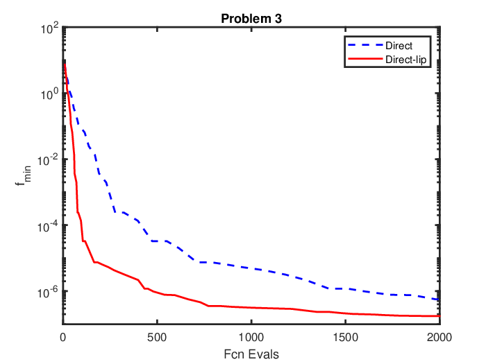
We finally show results on the Problems 2–6 from paper [19]. In order to consider only affine VIs, we dropped the absolute value in the operator of Problems 4 and 5. In Table 1, we report, for each problem, the number of function evaluations needed by the two algorithms to reach a certain gap value (we chose , , ). As we can easily see, the number of function evaluations is usually smaller for -DIRECT (we report in red the cases where -DIRECT needs a higher number of evaluations). In Figure 3, we further report the plots related to the gap reduction with respect to the number of function evaluations used for Problems 3 and 4. We indicate with the gap value (reported on the axis) and with Fcn Evals the number of function evaluations (reported on the axis). As we can see, the use of the Lipschitz constant estimate significantly speeds up the algorithm.

| DIRECT | -DIRECT | ||||||
| Problem | |||||||
| 2 | 3 | 125 | 431 | 977 | 97 | 313 | 749 |
| 3 | 4 | 115 | 277 | 711 | 49 | 77 | 165 |
| 4 | 3 | 79 | 269 | 1479 | 97 | 223 | 891 |
| 5 | 5 | 383 | 1913 | 1969 | 365 | 1961 | 2000 |
| 6 | 10 | 1987 | 1987 | 1987 | 875 | 1341 | 1799 |
6 Conclusions
In this paper, we propose a global optimization approach for solving general EPs without assuming any monotonicity-type condition on . This approach is based on two phases: (i) reformulate an EP as a global optimization problem via gap functions; (ii) use an improved version of the DIRECT algorithm, which exploits local bounds of the Lipschitz constant of the objective function, combined with local searches to solve the considered global optimization problem. Moreover, we provide some general results on Lipschitz continuity of gap functions and, for some special classes of EPs, show simple estimates of their Lipschitz constants that can be exploited in the improved DIRECT algorithm. Preliminary numerical experiments on a set of instances from the literature and sets of randomly generated instances show the effectiveness of our approach for solving non-monotone EPs.
Acknowledgments.
The work of M. Passacantando and F. Rinaldi has been partially supported by the Italian Government project PRIN2015B5F27W “Nonlinear and Combinatorial Aspects of Complex Networks”. M. Passacantando is member of the Gruppo Nazionale per l’Analisi Matematica, la Probabilità e le loro Applicazioni (GNAMPA - National Group for Mathematical Analysis, Probability and their Applications) of the Istituto Nazionale di Alta Matematica (INdAM - National Institute of Higher Mathematics).
References
- [1] F.A. Al-Khayyal. An implicit enumeration procedure for the general linear complementarity problem. Math. Programming Stud., (31):1–20, 1987.
- [2] G. Bigi, M. Castellani, M. Pappalardo, and M. Passacantando. Existence and solution methods for equilibria. European Journal of Operational Research, 227(1):1–11, 2013.
- [3] G. Bigi and M. Passacantando. Twelve monotonicity conditions arising from algorithms for equilibrium problems. Optimization Methods and Software, 30(2):323–337, 2015.
- [4] E. Blum and W. Oettli. From optimization and variational inequalities to equilibrium problems. Math. student, 63:123–145, 1994.
- [5] R. Burachik and G. Kassay. On a generalized proximal point method for solving equilibrium problems in Banach spaces. Nonlinear Analysis: Theory, Methods & Applications, 75(18):6456–6464, 2012.
- [6] O. Chadli, I.V. Konnov, and J.C. Yao. Descent methods for equilibrium problems in a Banach space. Computers & Mathematics with Applications, 48(3-4):609–616, 2004.
- [7] D. Di Lorenzo, M. Passacantando, and M. Sciandrone. A convergent inexact solution method for equilibrium problems. Optimization Methods and Software, 29(5):979–991, 2014.
- [8] G. Di Pillo, G. Liuzzi, S. Lucidi, V. Piccialli, and F. Rinaldi. A DIRECT-type approach for derivative-free constrained global optimization. Computational Optimization and Applications, 65(2):361–397, 2016.
- [9] K. Fan. A minimax inequality and applications. Inequalities, 3:103–113, 1972.
- [10] S.D. Flåm and A.S. Antipin. Equilibrium programming using proximal-like algorithms. Mathematical Programming, 78(1):29–41, 1996.
- [11] R. Horst, P.M. Pardalos, and N. Van Thoai. Introduction to Global Optimization. Introduction to Global Optimization. Springer US, 2000.
- [12] D.R. Jones, C.D. Perttunen, and B.E. Stuckman. Lipschitzian optimization without the Lipschitz constant. Journal of optimization Theory and Applications, 79(1):157–181, 1993.
- [13] I.V. Konnov. Application of the proximal point method to nonmonotone equilibrium problems. Journal of Optimization Theory and Applications, 119(2):317–333, 2003.
- [14] I.V. Konnov and O.V. Pinyagina. D-gap functions for a class of equilibrium problems in Banach spaces. Computational Methods in Applied Mathematics Comput. Methods Appl. Math., 3(2):274–286, 2003.
- [15] N. Langenberg. Interior proximal methods for equilibrium programming: part I. Optimization, 62(9):1247–1266, 2013.
- [16] N. Langenberg. Interior proximal methods for equilibrium programming: part II. Optimization, 62(12):1603–1625, 2013.
- [17] G. Liuzzi, S. Lucidi, and V. Piccialli. Partitioning techniques for global optimization. In V. De Simone, D. Di Serafino, and G. Toraldo, editors, Recent Advances in Nonlinear Optimization and Equilibrium Problems: A Tribute to Marco D’Apuzzo, volume 27 of Quaderni di Matematica, Dipartimento di Matematica, Seconda Università di Napoli, pages 253–272. Aracne Editrice S.r.l., 2012.
- [18] S. Lucidi and M. Sciandrone. A derivative-free algorithm for bound constrained optimization. Computational Optimization and applications, 21(2):119–142, 2002.
- [19] M. Majig, B. Barsbold, R. Enkhbat, and M. Fukushima. A global optimization approach for solving non-monotone variational inequality problems. Optimization, 58(7):871–881, 2009.
- [20] M. Majig, A.R. Hedar, and M. Fukushima. Hybrid evolutionary algorithm for solving general variational inequality problems. Journal of Global Optimization, 38(4):637–651, 2007.
- [21] G. Mastroeni. Gap functions for equilibrium problems. Journal of Global Optimization, 27(4):411–426, 2003.
- [22] G. Mastroeni. On auxiliary principle for equilibrium problems. In Equilibrium problems and variational models, pages 289–298. Springer, 2003.
- [23] J.J. Moré and S.M. Wild. Benchmarking derivative-free optimization algorithms. SIAM Journal on Optimization, 20(1):172–191, 2009.
- [24] A. Moudafi. Proximal point algorithm extended to equilibrium problems. Journal of Natural Geometry, 15(1-2):91–100, 1999.
- [25] L.D. Muu and T.D. Quoc. Regularization algorithms for solving monotone Ky Fan inequalities with application to a Nash-Cournot equilibrium model. Journal of optimization theory and applications, 142(1):185–204, 2009.
- [26] T.T.V. Nguyen, J.-J. Strodiot, and V.H. Nguyen. A bundle method for solving equilibrium problems. Mathematical programming, 116(1-2):529–552, 2009.
- [27] M. Pappalardo, G. Mastroeni, and M. Passacantando. Merit functions: a bridge between optimization and equilibria. Annals of Operations Research, 240(1):271–299, 2016.
- [28] P.M. Pardalos and J.B. Rosen. Global optimization approach to the linear complementarity problem. SIAM Journal on Scientific and Statistical Computing, 9(2):341–353, 1988.
- [29] T.D. Quoc, L.D. Muu, and V.H. Nguyen. Extragradient algorithms extended to equilibrium problems. Optimization, 57(6):749–776, 2008.