False Discovery Rate Control Under General Dependence By Symmetrized Data Aggregation
Abstract
We develop a new class of distribution–free multiple testing rules for false discovery rate (FDR) control under general dependence. A key element in our proposal is a symmetrized data aggregation (SDA) approach to incorporating the dependence structure via sample splitting, data screening and information pooling. The proposed SDA filter first constructs a sequence of ranking statistics that fulfill global symmetry properties, and then chooses a data–driven threshold along the ranking to control the FDR. The SDA filter substantially outperforms the knockoff method in power under moderate to strong dependence, and is more robust than existing methods based on asymptotic -values. We first develop finite–sample theories to provide an upper bound for the actual FDR under general dependence, and then establish the asymptotic validity of SDA for both the FDR and false discovery proportion (FDP) control under mild regularity conditions. The procedure is implemented in the R package sdafilter. Numerical results confirm the effectiveness and robustness of SDA in FDR control and show that it achieves substantial power gain over existing methods in many settings.
Keywords: Empirical distribution; Integrative multiple testing; Moderate deviation theory; Sample-splitting; Uniform convergence.
1 Introduction
Multiple testing provides a useful approach to identifying sparse signals from massive data. Recent developments on false discovery rate (FDR; Benjamini and Hochberg 1995) methodologies have greatly influenced a wide range of scientific disciplines including genomics (Tusher et al. 2001; Roeder and Wasserman 2009), neuroimaging (Pacifico et al. 2004; Schwartzman et al. 2008), geography (Caldas de Castro and Singer 2006; Sun et al. 2015) and finance (Barras et al. 2010). Conventional FDR procedures, such as the Benjamini–Hochberg (BH) procedure, adaptive -value procedure (Benjamini and Hochberg 1997) and adaptive -value procedure based on local FDR (Efron et al. 2001; Sun and Cai 2007), are developed under the assumption that the test statistics are independent. However, data arising from large–scale testing problems are often dependent. FDR control under dependence is a critical problem that requires much research. Two key issues include (a) how the dependence may affect existing FDR methods, and (b) how to properly incorporate the dependence structure into inference.
1.1 FDR control under dependence
The impact of dependence on FDR analysis was first investigated by Benjamini and Yekutieli 2001, who showed that the BH procedure, when adjusted at level with being the number of tests, controls the FDR at level under arbitrary dependence among the -values. However, this adjustment is often too conservative in practice. Benjamini and Yekutieli 2001 further proved that applying BH without any adjustment is valid for FDR control for correlated tests satisfying the PRDS property. This result was strengthened by Sarkar 2002, who showed that the FDR control theory under positive dependence holds for a generalized class of step-wise methods. Storey et al. 2004, Wu 2008 and Clarke and Hall 2009 respectively showed that, in the asymptotic sense, BH is valid under weak dependence, Markovian dependence and linear process models. Although controlling the FDR does not always require independence, some key quantities in FDR analysis, such as the expectation and variance of the number of false positives, may possess substantially different properties under dependence (Owen 2005; Finner et al. 2007). This implies that conventional FDR methods such as BH can suffer from low power and high variability under strong dependence. Efron 2007 and Schwartzman and Lin 2011 showed that strong correlations degrade the accuracy in both estimation and testing. In particular, positive/negative correlations can make the empirical null distributions of -values narrower/wider, which has substantial impact on subsequent FDR analyses. These insightful findings suggest that it is crucial to develop new FDR methods tailored to capture the structural information among dependent tests.
Intuitively high correlations can be exploited to aggregate weak signals from individuals to increase the signal to noise ratio (SNR). Hence informative dependence structures can become a bless for FDR analysis. For example, the works of Benjamini and Heller 2007, Sun and Cai 2009 and Sun and Wei 2011 showed that incorporating functional, spatial, and temporal correlations into inference can improve the power and interpretability of existing methods. However, these methods are not applicable to general dependence structures. Efron 2007, Efron 2010 and Fan et al. 2012 discussed how to obtain more accurate FDR estimates by taking into account arbitrary dependence. For a general class of dependence models, Leek and Storey 2008, Friguet et al. 2009, Fan et al. 2012 and Fan and Han 2017 showed that the overall dependence can be much weakened by subtracting the common factors out, and factor–adjusted -values can be employed to construct more powerful FDR procedures. The works by Hall and Jin 2010, Jin 2012 and Li and Zhong 2017 showed that, under both the global testing and multiple testing contexts, the covariance structures can be utilized, via transformation, to construct test statistics with increased SNR, revealing the beneficial effects of dependence. However, the above methods, for example by Fan and Han 2017 and Li and Zhong 2017, rely heavily on the accuracy of estimated models and the asymptotic normality of the test statistics. Under the finite–sample setting, poor estimates of model parameters or violations of normality assumption may lead to less powerful and even invalid FDR procedures. This article aims to develop a robust and assumption–lean method that effectively controls the FDR under general dependence with much improved power.
1.2 Model and problem formulation
We consider a setup where -dimensional vectors , , follow a multivariate distribution with mean and covariance matrix . The problem of interest is to test hypotheses simultaneously:
The summary statistic obeys a multivariate normal (MVN) model asymptotically
| (1) |
Denote the precision matrix. We first assume that is known. For the case with unknown precision matrix, a data-driven methodology and its theoretical properties are discussed in Section 4. The problem of multiple testing under dependence can be recast as a variable selection problem in linear regression. Specifically, by taking a “whitening” transformation, Model (1) is equivalent to the following model:
| (2) |
where is the pseudo response, is the design matrix, is a -dimensional identity matrix and are noise terms that are approximately independent and normally distributed. The connection between model selection and FDR was discussed in Abramovich et al. 2006 and Bogdan et al. 2015, respectively under the normal means model and regression model with orthogonal designs.
Let , , where is an indicator function, and corresponds to a null/non-null variable. Let be a decision, where indicates that is rejected and otherwise. Let denote the non–null set and the null set. The set of coordinates selected by a multiple testing procedure is denoted . Define the false discovery proportion (FDP) and true discovery proportion (TDP) as:
| (3) |
where . The FDR is the expectation of the FDP: . The average power is defined as .
1.3 FDR control by symmetrized data aggregation
This article introduces a new information pooling strategy, the symmetrized data aggregation (SDA), for handling the dependence issue in multiple testing. The SDA involves splitting and reassembling data to construct a sequence of statistics fulfilling symmetry properties. Our proposed SDA filter for FDR control consists of three steps:
- •
The first step splits the sample into two parts, both of which are utilized to construct statistics to assess the evidence against the null.
- •
The second step aggregates the two statistics to form a new ranking statistic fulfilling symmetry properties.
- •
The third step chooses a threshold along the ranking by exploiting the symmetry property between positive and negative null statistics to control the FDR.
To get intuitions on how the idea works, we start with the independent case [Zou et al. 2020]. The more interesting but complicated dependent case will be described shortly, with detailed discussions, refinements and justifications deferred to later sections. Suppose the vectors are i.i.d. obeying . The proposed SDA method first splits the full sample into two disjoint subsets and , with sizes and and . A pair of statistics, both of which follow under the null, are then calculated to test :
The product is used to aggregate the evidence across the two groups. If is large, then both and tend to have large absolute values with the same sign, thereby leading to a positive and large . By contrast, fulfills the symmetry property under , i.e.
| , for any | (4) |
This motivates one to consider the following selection procedure , where is the threshold chosen to control the FDR at level :
| (5) |
According to the symmetry property (4), the count of negative ’s below strongly resembles the count of false positives in the selected subset (i.e. the null ’s above ). It follows that the fraction in Equation (5) provides a good estimate of the FDP.
The dependent case involves a more carefully designed SDA filter. After sample splitting, we apply variable selection techniques such as LASSO to to construct . , which is calculated based on linear model (2), can effectively capture the dependence structure. Before using to construct , we carry out a data screening step to narrow down the focus. We show that the screening step can significantly increase the SNR of under strong dependence, hence the correlations are exploited again to increase the power. The ranking statistic is constructed by combining and with proven asymptotic symmetry properties. The theory of the proposed SDA filter is divided into two parts: the finite sample theory provides an upper bound for the FDR under general dependence, while the asymptotic theory shows that both the FDR and FDP can be controlled at under mild regularity conditions.
1.4 Connections to existing work and our contributions
The SDA is closely related to existing ideas of sample–splitting (Wasserman and Roeder 2009; Meinshausen et al. 2009) and data carving (Fithian et al. 2014; Lei et al. 2021), both of which firstly divide the data into two independent parts, secondly use one part to narrow down the focus (or rank the hypotheses) and finally use the remainder to perform inference tasks such as variable selection, estimation or multiple testing. These ideas have a common theme with covariate–assisted multiple testing (Lei and Fithian 2018; Cai et al. 2019; Li and Barber 2019), where the primary statistic plays the key role to assess the significance while the side information plays an auxiliary role to assist inference [see also the discussion by Ramdas 2019]. SDA provides a novel way of data aggregation where both parts of data, which are combined under the symmetry principle, play essential roles in both ranking and selection. This substantially reduces the information loss in conventional sample–splitting methods, while the symmetry principle, which is fulfilled by construction, enables the development of an effective and assumption-lean FDR filter.
The SDA is inspired by the elegant knockoff filter for FDR control (Barber and Candès 2015), which creates knockoff features that emulate the correlation structure in original features, to form symmetrized ranking statistics for selecting important variables via the same mechanism (5). The knockoff method, which is originally developed under regression models, can be applied for FDR control in Model (1) via the equivalent Model (2). The knockoff filter employs local pairwise contrasts: the ranking variable is constructed to capture the differential evidences against the null exhibited by the pair (i.e. the original feature vs. its knockoff copy). While it is desirable to make the pair as “independent” as possible, high correlations will greatly restrict the geometric space in which the knockoff can be constructed; see Appendix B.1 for detailed discussions and illustrations. This would significantly increase the difficulty for distinguishing the variable and its knockoff and hence lower the power. By contrast, the SDA filter, which does not rely on pairwise contrasts, will not suffer from high correlations.
To visualize the correlation effects, we consider a setup similar to Figure 5 in Barber and Candès 2015, where correlated normal, , and exponential data are generated based on an autoregressive model (see Section 5.2 for more details about the setup). We vary from to and apply BH, knockoff and SDA at FDR level . The actual FDRs and APs based on 500 replications are summarized in Figure 1. Our first column (normal data) shows that knockoff outperforms BH in some situations, but both the FDR and AP of the knockoff method decrease when correlations grow higher. By contrast, SDA controls the FDR near the nominal level consistently, and the power of SDA increases sharply with growing correlations. This pattern corroborates the insights by Benjamini and Heller 2007, Sun and Cai 2009 and Hall and Jin 2010 that high correlations, which can be exploited to increase the SNR, may become a bless in large–scale inference.

The proposed research improves the previous work by Zou et al. 2020 in several ways. First, Zou et al. 2020 has mainly focused on the independent and weak dependent case, with the major goal of deriving convergence rate of false discovery proportions when simultaneously performing thousands of -tests. The methodology in Zou et al. 2020, which does not utilize LASSO and does not include the data screening step, becomes highly inefficient under strong dependence. See Appendix B.2 for an illustration. Second, our new theories for FDR and FDP control under dependence and the robustness of the SDA filter under model misspecification substantially depart from the theory in Zou et al. 2020.
The SDA filter provides a model–free framework that overcomes the limitations of many selective inference procedures, for example, the methods in Lockhart et al. 2014 and Javanmard and Javadi 2019, which require strong assumptions about the conditional distribution to construct asymptotic -values. Our numerical results show that the methods in Fan and Han 2017 and Li and Zhong 2017, which require correctly specified models, accurate estimates of parameters and normality assumptions, are in general not robust for FDR control. The SDA filter, which employs empirical distributions instead of asymptotic distributions, only requires the global symmetry of the ranking statistics. It is more robust than its competitors for a wide range of scenarios since the asymptotic symmetry property is much easier to achieve in practice compared to asymptotic normality11 1 For example, the average of several -variables fulfills the symmetry property perfectly but violates the normality assumption. For asymmetric distributions such as exponential, we usually need a smaller sample size to achieve asymptotic symmetry compared to asymptotic normality – the latter is stronger than the former since it requires an additional accurate approximation in the tail areas.. As illustrated by the second column (multivariate data) of Figure 1, BH fails to control the FDR under heavy–tailed models. The failure in accounting for the deviations from normality may result in misleading empirical null and severe bias in FDR analysis (Efron 2004; Delaigle et al. 2011; Liu and Shao 2014). Finally, our Theorem 1, which develops a finite–sample upper bound of FDR under dependence, is closely connected to robust knockoffs theory and is established utilizing key arguments from Barber et al. 2020. More specifically, we employ the leave-one-out technique suggested in Barber et al. 2020 to analyze the effect on the SDA filter of possible deviations from normality and the sure screening property, similarly to the analysis of the effect on the Model-X knockoff filter of errors in estimating the true covariance structure. This important connection sheds lights on how the model uncertainty can affect the actual FDR level and how the error bound in FDR can be explicitly quantified using appropriate deviation measures; a detailed discussion is provided in Section B.3 of the Supplementary Material.
1.5 Organization
The remainder of our paper is structured as follows. In Section 2, we introduce the SDA filter for FDR control and discuss the effects of dependence on multiple testing. We develop finite sample and asymptotic theories for FDR control in Section 3. Methodology and theory for the unknown dependence case are discussed in Section 4. Simulation and real data analysis are presented in Sections 5 and 6, respectively. The extensions, proofs of theories and additional comparisons are provided in the Supplementary Material.
Notations. For , let be the design matrix with columns and being the th column. For a matrix or a vector , is similarly defined. Let be the norm, , and . Let and denote the smallest and largest eigenvalues of a square matrix . The notation means that and are both bounded in probability as . The “” and “” are similarly defined. Let denote the two quantities are asymptotically equivalent, in the sense that .
2 The SDA Filter for FDR Control
We start with the assumption that the covariance matrix is known and then move to the case with unknown in Section 4. Our discussion is mainly based on regression model (2); an equivalent description of the methodology via model (1) follows similarly. We first outline in Section 2.1 the steps for constructing the ranking statistics, then provide intuitive explanations on how the SDA filter works in Sections 2.2 and 2.3. The detailed SDA algorithm is provided in Section A.4.
2.1 Construction of ranking statistics and the symmetry property
SDA first splits the data into two independent parts and , which are respectively used to construct statistics and . The information in the two parts is then combined to form the ranking statistic . A wide class of pairs may be constructed from the sample. This section presents a specific pair , which is used in all numerical studies. Examples of other possible pairs are presented in Section A.2 in the Supplementary Material.
We propose to use LASSO (Tibshirani 1996) to extract information from as it simultaneously takes into account the sparsity and dependency structures. Let and . The LASSO estimator is given by , where
| (6) |
Let denote the subset of coordinates selected by LASSO and its complement.
Remark 1
Following Wasserman and Roeder 2009, we suggest using , which provides stable performance across a wide range of settings. To obtain asymptotically unbiased estimator in the next step, it is required that contains all the signals with high probability. In practice, this can be achieved by deliberately choosing an overfitted model that includes most true signals and many false positives; see also Barber and Candès 2019 and Remark 2 in Section 3.2.
Next we use to obtain the least–squares estimates (LSEs). Let , , and 22 2 Specifically, is an -vector with 1 in the th coordinate and 0 elsewhere.. The LSEs are only calculated for coordinates on the narrowed subset . Let , where
Section 2.3 provides insights on why this data screening step can lead to increased SNR.
To aggregate information across both and , let , where
| (9) |
and ’s are the diagonal elements of . A multiple testing procedure consists of two steps: ranking and thresholding. Next we show that ’s play key roles in both steps. Intuitively, the positive ’s can be used for ranking because a large and positive indicates strong evidence against the null. Meanwhile, the negative ’s, which usually correspond to null cases, can be used for thresholding. The key idea is to exploit the following asymptotic symmetry property:
| (10) |
which holds if 33 3 We shall see that contains all signals, then the LSEs of the null coordinates are symmetrically distributed around 0. Hence ’s satisfy (4). It is easy to see that (10) is an asymptotic version of the symmetry property given by (4); see Lemmas S.1-S.2 in Section C of the Supplementary Material for a rigorous discussion.. Next we explain how the SDA filter works.
2.2 FDR thresholding
The asymptotic symmetry property (10) motivates us to choose the following data–driven threshold to control the FDR at level :
| (11) |
Our decision rule is given by Denote the discovery set. To see why (11) makes sense, note that is an overestimation of , which is asymptotically equal to , the number of false positives, due to the asymptotic symmetry property (10). It follows that the fraction in (11) provides an overestimate of the FDP, which (desirably) leads to a conservative FDR control. Moreover, the empirical FDR level is typically very close to because the gap between the fraction in (11) and the actual FDP is usually small in practice, where, for a suitably chosen , most cases in should come from the null.
The operation of the SDA filter can be visualized in Figure 2. We generate from an MVN distribution with and . We randomly set 10% of the coordinates in to be and 0 elsewhere. Panel (a) presents the scatter plot of 288 nonzero ’s with red triangles and black dots respectively denoting true signals and nulls. Panel (d) plots the normalized knockoff statistics that are constructed according to (1.7) in Barber and Candès 201544 4 The normalization, which makes the plot easier to read, does not affect the results of the knockoff method. This is because only the relative magnitudes of matter in the thresholding step of the knockoff method.. We can see that both SDA and knockoff fulfill the symmetry property approximately for the null ’s (black dots). However, SDA achieves a more clearcut separation of signals and noise. As explained in Section B.1 of the Supplement, the symmetrized knockoff statistics suffers from high correlations. By contrast, the construction of SDA statistic, which does not depend pairwise contrasts, eliminates the needs for creating fake variables. We can see from Panel (a) that the SDA ranking places most true signals above 0, and many true signals stay well above the majority of the null cases. However, in Panel (d) that illustrates the knockoff ranking, the true signals are not well separated from the nulls, and many true signals even fall below 0. Since the threshold must be positive, signals with negative ’s will be missed, which leads to substantial power loss.
The impacts on the FDP processes are shown in the second column in Figure 2. We can see that the estimated FDP process [] of SDA approximates the true FDP process [] fairly accurately. However, the knockoff method yields overly conservative estimates of the true FDPs, which leads to overly conservative thresholds (marked by blue vertical lines). The last column in Figure 2 compares the TDP processes of SDA and knockoff. At the FDR level 0.2, the TDP of SDA is 0.87 (threshold ), which is much higher than that of knockoff (TDP=0.03 with threshold ). The low TDP of knockoff is due to the decreased power in distinguishing the signal from noise [Panel (d)] and an overly conservative threshold [Panel (e)].

2.3 Power and effects of dependence
The impact of dependence on FDR analysis has been extensively studied but most discussions have focused on the validity issue. This section first discusses the impact of dependence on power, and then provides insights on the information loss of conventional data splitting methods.
Under the SDA framework, many possible pairs of may be constructed. It is easy to show that constructed via the pairs of sample averages
| (12) |
also fulfill the asymptotic symmetry property. However, the pair in (12), which falls into the class of marginal testing techniques, can be highly inefficient since it completely ignores the dependence structure. Next we provide intuitions on how the dependence structure is incorporated into the SDA filter to improve the efficiency of existing methods.
First, is superior to by leveraging joint modeling techniques. The merit of joint modeling has been carefully illustrated by Barber and Candès 2015 through extensive simulations. Candès et al. 2018 further argued that the conditional testing techniques are in general more powerful in recovering sparse signals than marginal testing methods. is constructed based on LASSO (a conditional inference technique) and serves as a more suitable building block than for constructing . Second, enjoys a higher SNR than by exploiting the dependence between and . Clearly, the expectations of both and are . The covariance of is , where . By the inversion formula of a block matrix, we have Hence, , which is the conditional covariance of given . Let be the -th element of . Then . However, This provides the key insight on the effect of data screening. In regression terms, strong correlations indicate that a large fraction of variability in the variables in can be explained by the variables in . The higher the correlations, the more reductions in the uncertainties and hence the higher SNRs. This explains why SDA becomes more powerful as correlations increase (Figure 1).
Finally, both knockoff and SDA achieve the symmetry property at the expense of possibly reduced SNR: the former increases the dimension of the design matrix by adding noise variables while the latter involves sample splitting. In contrast with the sample splitting method in Wasserman and Roeder 2009, where is thrown away after model selection, SDA provides a new aggregation strategy: is kept and combined with to form the ranking statistic . This substantially reduces the information loss in conventional sample splitting methods.
2.4 Effects of data screening
The data screening step is always beneficial as long as the tests are correlated. Intuitively, the smaller the set , the larger amount of uncertainty can be explained by the variables in . Hence a more effective dimension reduction implies increased SNR and higher power. Meanwhile, our theory on FDR control requires that holds with high probability, indicating that an overly aggressive data screening step can hurt the FDR procedure. In practice, we recommend deliberately choosing an overfitted model to ensure the validity in FDR control; this would slightly compromise the power. To illustrate the tradeoff, Figure 3 presents a numerical study to investigate how the size of may affect both the FDR and power. We can see that the actual FDRs of SDA may deviate from the nominal level when is too small. By contrast, a large (overfitted model) has little impact on the FDR levels, but affects the power negatively.

3 Theoretical Properties of the SDA Filter
This section first establishes finite sample theory for FDR bounds (Section 3.1), and then develops asymptotic theories for FDR and FDP control.
3.1 Finite–sample theory on FDR control
Our finite–sample theory, which requires no model assumptions, establishes an upper bound for the FDR under general dependence. We emphasize that the upper bound holds for both known and estimated covariance matrices.
Our theory is developed for a modified SDA filter (SDA+) which chooses the threshold
SDA+ is slightly more conservative than SDA but their difference is negligible when the number of rejections is large. Recall . Denote and . The key quantity that controls the upper bound is
| (13) |
which can be interpreted as a measure of the extent to which the “flip–sign” property of is violated55 5 For a null variable (i.e. ), the flip–sign property means that is equally likely to be positive or negative conditioning on its magnitude and other ’s in .. Our finite sample theory for FDR control is given by Theorem 1.
Theorem 1
For any , the FDR of the SDA+ method satisfies
| (14) |
Our theorem is closely connected to Theorem 1 in Barber et al. 2020. Both theorems involve assessing how the deviations from the “idealized situation” would affect the actual FDR level. However, the interpretations are very different. In model-X knockoff the deviation (from the assumption of a known X matrix) comes from the estimation errors of the X matrix whereas in SDA the deviation (from the perfect symmetry property) comes from the possible violations of the normality assumption and sure screening property. Our theorem shows that a tight control of ’s leads to effective FDR control. Next we carefully interpret the bound and present several important settings in which the upper bound in (14) exactly achieves or is very close to the nominal level .
Consider the ideal case where (a) the error distribution is symmetric, (b) contains all signals and (c) ’s are independent of each other for . We can show that for all . The upper bound achieves the nominal level exactly since and hence we can set . Even when the error distribution is asymmetric, we expect that ’s would become vanishingly small for moderate sample size due to the convergence of to a symmetric distribution (Lemma S.1). Hence the FDR bound would be close to .
Next we turn to the dependent case. For simplicity, assume that ’s come from a multivariate normal distribution. Let with . The matrix is the conditional covariance matrix of given . The following lemma shows that the magnitude of is controlled by the matrix .
Lemma 1
(Flip–sign property under Gaussian dependence). Assume that ’s obey a multivariate normal distribution. Denote the th column of excluding . If , then .
To provide some intuitions on how close the bound is to in practice, consider the autoregressive (AR) structure . Since the precision matrix of AR structure is tridiagonal, only consecutive coordinates are correlated with each other conditional on remaining variables. Suppose sparse signals are randomly distributed on the coordinates and the dimension reduction via is performed effectively, e.g. . Let be an event such that for any null variable , remaining variables in are conditionally uncorrelated with it. We expect to occur with high probability since for large tridiagonal precision matrices, there is a small chance that two consecutive coordinates are selected into a small set simultaneously. On event , we have and it follows from Lemma 1 that . Consequently the FDR bound would converge to when . In the same vein, we expect that the bound would be close to for the class of power decay covariance matrices and the class of sparse precision matrices.
3.2 Asymptotic theory on FDP control
Under the asymptotic paradigm we can prove that the FDR can be controlled at under suitable conditions (asymptotic validity). Denote . Let , , and . Assume that is uniformly bounded above by some non-random sequence that will be specified later. We start with some regularity conditions.
Condition 1
(Sure screening property) As , .
Remark 2
Condition 1 ensures that is unbiased for . This pre–selection property, which has been commonly used (Wasserman and Roeder 2009; Meinshausen et al. 2009; Barber and Candès 2019), can be fulfilled with suitably chosen under the “zonal” assumption (Bühlmann and Mandozzi 2014). In practice, we recommend applying AIC to deliberately choose an overfitted model. The sure screening property may not hold exactly but missing small ’s is inconsequential. For example, if we ignore “unimportant” signals, then Condition 1 is fulfilled by LASSO for large signals exceeding the rate of . Asymptotically unbiased estimators are usually sufficient for effective FDR control. This has been corroborated by our empirical results in Section 5.
Condition 2
(Estimation accuracy) The estimator fulfills , where is a sequence satisfying and .
Remark 3
Condition 2 assumes that is a reasonable estimator of ; this condition typically holds with for the LASSO solution (Van de Geer and Bühlmann 2009).
The next two conditions are standard: Condition 3 imposes constraints on the diverging rates of and , both of which depend on the existence of certain moments; Condition 4 requires that the eigenvalues of the design matrix are doubly bounded by two constants.
Condition 3
(Moments) There exist two positive diverging sequences and such that and uniformly in and , where . Assume that as , , for some small .
Condition 4
(Covariance) There exist positive constants and such that with probability one,
Condition 5
(Signals) As , , where
Remark 4
Condition 5 implies that the number of identifiable effect sizes should not be too small as . This seems to be a necessary condition for FDP control. For example, Liu and Shao 2014 showed that if a multiple testing method controls the FDP with high probability, then its number of true alternatives must diverge when the number of tests goes to infinity.
Condition 6
(Dependence) Let . Assume that for each , , where , is any small constant, and as .
Remark 5
Condition 6 allows to be correlated with all others but requires that the number of large correlations cannot diverge too fast. The condition appears to be similar to the regularity conditions in Fan et al. 2012 and Xia et al. 2020 but in fact our condition is much weaker. For instance, the correlation between and is just the partial correlation of and given the rest variables. In particular, large correlations would be highly unlikely after data screening for a wide range of popular models, such as the class of power decay covariance matrices and the class of moderately sparse precision matrices. This reveals the advantage of SDA, which effectively de–correlates the strong dependence via data screening and conditioning.
Our main theoretical result on the asymptotic validity of the SDA method for both FDP and FDR control is given by the next theorem.
4 Unknown dependence
Now we turn to the case where the covariance structure is unknown. When is unknown, the SDA filter operates in the same way except that we substitute the estimate in place of .
We propose to estimate using only the first part of the sample . Denote the corresponding estimator. Then the SDA filter can be readily constructed via the steps in Sections 2.1-2.2 with . Various high-dimensional precision matrix estimation methods, such as the graphical LASSO (Friedman et al. 2008) and CLIME (Cai et al. 2011), can be used to obtain . An attractive feature of the SDA filter under unknown dependence is its robustness for FDR control. We next show that the SDA filter is robust for FDR control if is constructed based only on . We first state a modified version of Condition 6, which uses in place of .
Condition 6’ Let and . Assume that for each , , where , is any small constant, and as .
The following theorem, which is in parallel with Theorem 2, establishes the asymptotic validity of the SDA filter for estimated covariance.
Theorem 3
Remark 6
Our FDR theory does not require an accurate estimator for . The accuracy of the estimator only affects the power but not the validity. Consider a working covariance structure that “estimates” as the identity matrix. Then it can be shown that the FDP can still be controlled. This is more attractive than the FDR theories in, for example, Fan and Han 2017 and Li and Zhong 2017 that critically depend on the accuracy of the covariance estimators.
The key step in the proof is to verify the validity of (10). This amounts to addressing two major issues: the asymptotic symmetry of under the null and the uniform convergence of . Because is obtained from , then is unbiased conditional on and thus is approximately equal to , establishing the symmetry property. The dependence assumption on ensures the convergence of .
While sample–splitting ensures the independence between and and hence the robustness of the SDA filter, as one would expect, a more accurate estimate of yields better power. Previously we have proposed to estimate using and construct the LSE (2.1) using . In practice one may consider using to construct , and then obtaining the LSE via the full sample estimator, denoted , that is estimated using . The caveat is that, although can potentially increase the power, stronger conditions will be needed to guarantee the asymptotic validity of the “full–sample” SDA method. As pointed out by an insightful referee, the asymptotic theory requires that must converge to at a very fast rate, which can be impractical in applications. We recommend the robust SDA filter that estimates using only . Next we specify the requirements on the estimation accuracy of .
Condition 7
The estimated precision matrix satisfies with .
The following theorem shows that the FDR and FDP can be controlled asymptotically when is sufficiently close to . Let .
Theorem 4
This theorem, which is a complementary result to Theorem 3, provides conditions that warrant the implementation of a more efficient version of SDA. It is worth further investigating the condition (16), which seems to be unavoidable because and are no longer independent when the whole sample is used to estimate . To fix ideas, suppose that is -sparse, i.e. , and that all its elements s are bounded. First, standard arguments in, for example, Yuan 2010 and Liu et al. 2012 indicate that . Accordingly, with , Equation (16) is equivalent to the condition if is of a polynomial rate of . The condition above imposes restrictions on the diverging rates of , , and . Assume that , and are all bounded. Then we must require that . Alternatively, if we only assume that and are bounded, then a sufficient condition for (16) is (since ). These rates are consistent with those in the literature; see, for example, Portnoy et al. 1984 and Fan and Peng 2004.
5 Simulation
This section first introduces the R package sdafilter (Section 5.1), followed by simulation designs (Section 5.2) and comparison results (Section 5.3). Additional results for comparisons with unknown covariance matrix and other correlation structures are provided in the Supplementary Material.
5.1 Implementation details
We describe the implementation details of the R package sdafilter. For sample–splitting, we follow the strategy in Wasserman and Roeder 2009, which uses for selecting variables, and the rest for obtaining the LSEs. The AIC is used to select the tuning parameter in LASSO. If the number of the variables selected by AIC exceeds , then only the first variables will be retained. For the case with unknown , our default option is to apply the R package glasso to , where the tuning parameter is set by the R package huge. If prior knowledge suggests a nonsparse , the “nonsparse” option in our package can be used. This option first estimates the covariance matrix using the R package POET and then takes its inverse as the input. The stable option implements the R-SDA method described in Section A.1 of the Supplementary Material. The kwd option enables the usage of different estimators to summarizes the information in the first part of data, including the de-biased LASSO, innovated transformation of the sample means (Hall and Jin 2010), and factor-adjusted sample means (Fan and Han 2017).
5.2 Simulation settings
We consider three types of covariance structures: (I) Autoregressive (AR) structure: . (II) Compound symmetry structure: all off-diagonal elements of the are , which can be regarded as a factor model with one principal component. (III) Sparse covariance structure: , where is a matrix and each row of has only one position with nonzero value sampled from uniform distribution .
The diagonal elements are normalized as unity for all three settings. To investigate the robustness of different methods, we consider three error distributions: (i) multivariate normal; (ii) -distribution with and (iii) exponential distribution with scale parameter 2. The observations are then standardized to have mean zero and standard deviation one. The correlation structure remains nearly unchanged after transformation. The following six methods will be compared:
- (a)
The Benjamini–Hochberg (BH) procedure with the -values transformed from the statistics.
- (b)
The principal factor approximation (PFA) procedure proposed by Fan et al. 2012 for known covariance and Fan and Han 2017 for estimated covariance. Two versions of the PFA procedure using the unadjusted -values and adjusted -values are implemented using the R package pfa, denoted as and respectively. We only report the results for as it generally outperforms .
- (c)
The sample-splitting method (SS; Wasserman and Roeder 2009), which conducts data screening using LASSO and then applies BH to the -values calculated based on .
- (d)
The knockoff method (Knockoff; Barber and Candès 2015), which is implemented using function “create.fixed” in the R package knockoff.
- (e)
The DATE method (DATE; Li and Zhong 2017), which we implemented by ourselves.
- (f)
The stability–refined SDA filter (R-SDA) implemented using our package sdafilter with the “stable” option. We only presented R-SDA, which we recommend to use in practice, to make the plots easier to read. SDA has similar performance to R-SDA.
Let be the sample size, the number tests, and the proportion of signals. For each combination , we generate data and apply the six methods at FDR level . The FDR and AP are calculated by averaging the proportions from 500 replications.
5.3 Comparison results for known covariance structures
We fix and generate from the following random mixture model:
where is the dirac delta function (denoting a point mass at 0), and is the density of the non-null distribution, specified as a uniform distribution . The signals ’s are then randomly multiplied by a flip-sign. To assess the effect of signal strength, we vary from to and apply the six methods to simulated data. The results for Structures (I) and (III) are summarized in Figure 4, where in the top row we fix . The results for Structure (II) with are shown in Figure S5 of the Supplementary Material. The following observations can be made.
- (a)
For the Gaussian error case, BH, knockoff, R-SDA and SS control the FDR at the nominal level. The FDR levels of and DATE are inflated when signals are weak.
- (b)
For the non-Gaussian error case, BH, DATE, SS and fail to control the FDR under various settings and the FDR levels can be much higher than the nominal level. Knockoff controls the FDR in all settings but can be very conservative. R-SDA has the most accurate and stable FDR levels among all methods.
- (c)
R-SDA vs SS and BH. As expected, SS and BH control the FDR under the Gaussian case but are not robust for non-Gaussian errors. R-SDA has much higher power than both methods (even when the FDR levels of R-SDA are much lower). It is interesting to note that although SS only uses the second part of the data, its power can be much higher than BH when the correlation structure is highly informative [Normal case under Structure (I) on top left]. This is because the data screening step can significantly increase the SNR (Section 2.3).
- (d)
R-SDA vs Knockoff. R-SDA and knockoff, both of which are distribution–free, are the only methods that can control the FDR at the nominal level across all scenarios. The knockoff method is overly conservative in Setting (I) due to the high correlation. The conservativeness become less severe under Setting (III). By contrast, R-SDA controls the FDR more accurately near the target level and has significantly higher power than knockoff.
- (e)
R-SDA vs DATE and . In some scenarios, DATE and can outperform SDA in power. However, the higher power may be attributed to the severely inflated FDRs. The numerical results reveal the promise of extending the SDA framework by employing other methods, such as factor–adjusted -scores or innovated transformations, as alternatives to the LASSO estimates, to construct .

Next we turn to investigate how the six methods are affected by the strength of correlation. For covariance structures (I) and (II), we fix under alternative and vary the magnitude of correlation from independence () to strong dependence (). The results are summarized in Figure 5. In addition to the observations that we have made based on the previous graph, the following additional patterns are worthy of mentioning.
- (a)
The knockoff method becomes more conservative when correlations become higher. Note that the average correlations in Structure (II) is much higher than that in Structure (I), the power of the knockoff method deteriorates faster for Structure (II) as increases. For Structure (II), the FDR of BH also decreases as increases.
- (b)
In contrast with BH and knockoff, both of which suffer from high correlations, the FDR of R-SDA remains at the nominal level consistently, and the power increases with the correlation. The power grows faster for Structure (II). This corroborates the insights that high correlations can be useful in FDR analysis (Benjamini and Heller 2007; Sun and Cai 2009).
- (c)
In Column 2 of Figure 5, knockoff fails to control the FDR for heavy tailed distributions when correlation is low. By contrast, SDA controls the FDR accurately under non-Gaussian errors.

6 A real-data example
This section illustrates the SDA filter for analysis of high-density oligonucleotide microarrays. The data set, which contains probe sets from 128 adult patients enrolled in the Italian GIMEMA multi–center clinical trial, has been used in Chiaretti et al. 2005 and Bourgon et al. 2010 for identifying genetic factors that are associated with acute lymphoblastic leukemia (ALL). The ALL dataset is available at http://www.bioconductor.org.
We focus on a subset of 79 patients with B-cell differentiation because existing research reveals that malignant cells in B-lineage ALL are often associated with genetic abnormalities that have significant impacts on the clinical course of the disease. The patients are divided into two groups based on the molecular heterogeneity of the B-lineage ALL: 37 with the BCR/ABL mutation and 42 with NEG. We further narrow down the focus to 10% of the genes (i.e., ) before carrying out the FDR analysis. Specifically, the uncorrelated screening method (Bourgon et al. 2010) has been used to remove probe sets with small overall sample variances since they are unlikely to be differentially expressed.

We apply a two–sample version of R-SDA (see Section A.3 for details), BH, SS, , Knockoff and DATE at several significance levels for identifying differentially expressed genes across the two groups. Table 1 summarizes the number of significant probe sets for each method. In Figure 6(a)-(b), we plot the pairwise correlations of the genes. We can see that a significant proportion of the correlations exceed 0.4. These correlations can jointly exhibit non-negligible dependence effect. This explains why the knockoff method is overly conservative. R-SDA is more powerful than SS by exploiting additional information from the second part of data. BH, and DATE claims more significant genes than R-SDA. However, some caveats need to be given regarding the reliability of BH, and DATE, which all require normality assumptions (and the latter two require accurate estimates of the unknown covariance matrices).
Next we conduct a preliminary analysis to investigate the normality assumption, which seems to have been severely violated in this data set. From Column 2 of Figure 6 we can see that the skewness scores of many genes exceed the conventional cutoff . As a comparison, we display in Column 3 of Figure 6 the “ideal” pattern where the normality assumption holds. The histograms in Column 2 are much wider than the histograms in Column 3, indicating a possibly highly skewed error distribution. One possible explanation for the difference in power is that BH, PFA-A and DATE may have inflated FDR levels under violation of normality. This has been observed in our simulation studies (e.g. last column in Figure S3). By contrast, SDA and knockoff are distribution–free methods, which tend to produce more reliable and replicable findings. The lists of 19 highest ranked probe sets by the six methods are presented in Table S1 of Appendix E.
| R-SDA | SS | BH | PFA-A | Knockoff | DATE | |
|---|---|---|---|---|---|---|
| 19 | 7 | 29 | 98 | 2 | 364 | |
| 33 | 15 | 146 | 182 | 2 | 452 | |
| 56 | 37 | 229 | 252 | 2 | 501 | |
| 139 | 68 | 350 | 339 | 7 | 546 |
Acknowledgments
The authors thank the Editor, Associate Editor and two anonymous referees for their many helpful comments that have resulted in significant improvements of the article.
References
- Abramovich et al. (2006) Abramovich, F., Benjamini, Y., Donoho, D. L., and Johnstone, I. M. (2006), “Adapting to unknown sparsity by controlling the false discovery rate,” The Annals of Statistics, 34, 584–653.
- Barber and Candès (2015) Barber, R. F. and Candès, E. J. (2015), “Controlling the false discovery rate via knockoffs,” The Annals of Statistics, 43, 2055–2085.
- Barber and Candès (2019) — (2019), “A knockoff filter for high-dimensional selective inference,” The Annals of Statistics, 47, 2504–2537.
- Barber et al. (2020) Barber, R. F., Candès, E. J., and Samworth, R. J. (2020), “Robust inference with knockoffs,” The Annals of Statistics, 48, 1409–1431.
- Barras et al. (2010) Barras, L., Scaillet, O., and Wermers, R. (2010), “False discoveries in mutual fund performance: Measuring luck in estimated alphas,” The journal of finance, 65, 179–216.
- Benjamini and Heller (2007) Benjamini, Y. and Heller, R. (2007), “False discovery rates for spatial signals,” Journal of the American Statistical Association, 102, 1272–1281.
- Benjamini and Hochberg (1995) Benjamini, Y. and Hochberg, Y. (1995), “Controlling the false discovery rate: a practical and powerful approach to multiple testing,” Journal of the Royal Statistical Society: Series B (Methodological), 57, 289–300.
- Benjamini and Hochberg (1997) — (1997), “Multiple Hypotheses Testing with Weights,” Scandinavian Journal of Statistics, 24, 407–418.
- Benjamini and Yekutieli (2001) Benjamini, Y. and Yekutieli, D. (2001), “The control of the false discovery rate in multiple testing under dependency,” The Annals of Statistics, 29, 1165–1188.
- Bickel and Levina (2008) Bickel, P. J. and Levina, E. (2008), “Regularized estimation of large covariance matrices,” The Annals of Statistics, 36, 199–227.
- Bogdan et al. (2015) Bogdan, M., Van Den Berg, E., Sabatti, C., Su, W., and Candès, E. J. (2015), “SLOPE-daptive variable selection via convex optimization,” The Annals of Applied Statistics, 9, 1103.
- Bourgon et al. (2010) Bourgon, R., Gentleman, R., and Huber, W. (2010), “Independent filtering increases detection power for high-throughput experiments,” Proceedings of the National Academy of Sciences, 107, 9546–9551.
- Bühlmann and Mandozzi (2014) Bühlmann, P. and Mandozzi, J. (2014), “High-dimensional variable screening and bias in subsequent inference, with an empirical comparison,” Computational Statistics, 29, 407–430.
- Cai and Liu (2016) Cai, T. and Liu, W. (2016), “Large-scale multiple testing of correlations,” Journal of the American Statistical Association, 111, 229–240.
- Cai et al. (2011) Cai, T., Liu, W., and Luo, X. (2011), “A constrained minimization approach to sparse precision matrix estimation,” Journal of the American Statistical Association, 106, 594–607.
- Cai et al. (2019) Cai, T. T., Sun, W., and Wang, W. (2019), “CARS: Covariate assisted ranking and screening for large-scale two-sample inference (with discussion),” Journal of the Royal Statistical Society: Series B (Methodological), 81, 187–234.
- Caldas de Castro and Singer (2006) Caldas de Castro, M. and Singer, B. H. (2006), “Controlling the false discovery rate: a new application to account for multiple and dependent tests in local statistics of spatial association,” Geographical Analysis, 38, 180–208.
- Candès et al. (2018) Candès, E., Fan, Y., Janson, L., and Lv, J. (2018), “Panning for gold: model-X knockoffs for high dimensional controlled variable selection,” Journal of the Royal Statistical Society: Series B (Methodological), 80, 551–577.
- Chiaretti et al. (2005) Chiaretti, S., Li, X., Gentleman, R., Vitale, A., Wang, K. S., Mandelli, F., Foa, R., and Ritz, J. (2005), “Gene expression profiles of B-lineage adult acute lymphocytic leukemia reveal genetic patterns that identify lineage derivation and distinct mechanisms of transformation,” Clinical cancer research, 11, 7209–7219.
- Clarke and Hall (2009) Clarke, S. and Hall, P. (2009), “Robustness of multiple testing procedures against dependence,” The Annals of Statistics, 37, 332–358.
- Delaigle et al. (2011) Delaigle, A., Hall, P., and Jin, J. (2011), “Robustness and accuracy of methods for high dimensional data analysis based on Student’s t-statistic,” Journal of the Royal Statistical Society: Series B (Methodological), 73, 283–301.
- Efron (2004) Efron, B. (2004), “Large-scale simultaneous hypothesis testing: the choice of a null hypothesis,” Journal of the American Statistical Association, 99, 96–104.
- Efron (2007) — (2007), “Correlation and large-scale simultaneous significance testing,” Journal of the American Statistical Association, 102, 93–103.
- Efron (2010) — (2010), “Correlated z-values and the accuracy of large-scale statistical estimates,” Journal of the American Statistical Association, 105, 1042–1055.
- Efron et al. (2001) Efron, B., Tibshirani, R., Storey, J. D., and Tusher, V. (2001), “Empirical Bayes analysis of a microarray experiment,” Journal of the American Statistical Association, 96, 1151–1160.
- Fan and Han (2017) Fan, J. and Han, X. (2017), “Estimation of the false discovery proportion with unknown dependence,” Journal of the Royal Statistical Society: Series B (Methodological), 79, 1143–1164.
- Fan et al. (2012) Fan, J., Han, X., and Gu, W. (2012), “Estimating false discovery proportion under arbitrary covariance dependence,” Journal of the American Statistical Association, 107, 1019–1035.
- Fan et al. (2013) Fan, J., Liao, Y., and Mincheva, M. (2013), “Large covariance estimation by thresholding principal orthogonal complements,” Journal of the Royal Statistical Society: Series B (Methodological), 75, 603–680.
- Fan and Peng (2004) Fan, J. and Peng, H. (2004), “Nonconcave penalized likelihood with a diverging number of parameters,” The Annals of Statistics, 32, 928–961.
- Finner et al. (2007) Finner, H., Dickhaus, T., and Roters, M. (2007), “Dependency and false discovery rate: asymptotics,” The Annals of Statistics, 35, 1432–1455.
- Fithian et al. (2014) Fithian, W., Sun, D., and Taylor, J. (2014), “Optimal inference after model selection,” arXiv preprint arXiv:1410.2597.
- Friedman et al. (2008) Friedman, J., Hastie, T., and Tibshirani, R. (2008), “Sparse inverse covariance estimation with the graphical lasso,” Biostatistics, 9, 432–441.
- Friguet et al. (2009) Friguet, C., Kloareg, M., and Causeur, D. (2009), “A factor model approach to multiple testing under dependence,” Journal of the American Statistical Association, 104, 1406–1415.
- Hall and Jin (2010) Hall, P. and Jin, J. (2010), “Innovated higher criticism for detecting sparse signals in correlated noise,” The Annals of Statistics, 38, 1686–1732.
- Javanmard and Javadi (2019) Javanmard, A. and Javadi, H. (2019), “False discovery rate control via debiased lasso,” Electronic Journal of Statistics, 13, 1212–1253.
- Jin (2012) Jin, J. (2012), “Comment,” Journal of the American Statistical Association, 107, 1042–1045.
- Leek and Storey (2008) Leek, J. T. and Storey, J. D. (2008), “A general framework for multiple testing dependence,” Proceedings of the National Academy of Sciences, 105, 18718–18723.
- Lei and Fithian (2018) Lei, L. and Fithian, W. (2018), “AdaPT: an interactive procedure for multiple testing with side information,” Journal of the Royal Statistical Society: Series B (Methodological), 80, 649–679.
- Lei et al. (2021) Lei, L., Ramdas, A., and Fithian, W. (2021), “A general interactive framework for false discovery rate control under structural constraints,” Biometrika, 108, 253–267.
- Li and Barber (2019) Li, A. and Barber, R. F. (2019), “Multiple testing with the structure-adaptive Benjamini–Hochberg algorithm,” Journal of the Royal Statistical Society: Series B (Methodological), 81, 45–74.
- Li and Zhong (2017) Li, J. and Zhong, P.-S. (2017), “A rate optimal procedure for recovering sparse differences between high-dimensional means under dependence,” The Annals of Statistics, 45, 557–590.
- Liu et al. (2012) Liu, H., Han, F., Yuan, M., Lafferty, J., and Wasserman, L. (2012), “High-dimensional semiparametric Gaussian copula graphical models,” The Annals of Statistics, 40, 2293–2326.
- Liu and Shao (2014) Liu, W. and Shao, Q.-M. (2014), “Phase transition and regularized bootstrap in large-scale -tests with false discovery rate control,” The Annals of Statistics, 42, 2003–2025.
- Lockhart et al. (2014) Lockhart, R., Taylor, J., Tibshirani, R. J., and Tibshirani, R. (2014), “A significance test for the lasso,” The Annals of Statistics, 42, 413–468.
- Meinshausen et al. (2009) Meinshausen, N., Meier, L., and Bühlmann, P. (2009), “P-values for high-dimensional regression,” Journal of the American Statistical Association, 104, 1671–1681.
- Owen (2005) Owen, A. B. (2005), “Variance of the number of false discoveries.” Journal of the Royal Statistical Society: Series B (Methodological), 67, 411–426.
- Pacifico et al. (2004) Pacifico, M. P., Genovese, C., Verdinelli, I., and Wasserman, L. (2004), “False Discovery Control for Random Fields,” Journal of the American Statistical Association, 99, 1002–1014.
- Petrov (2002) Petrov, V. (2002), “On probabilities of moderate deviations,” Journal of Mathematical Sciences, 109, 2189–2191.
- Portnoy et al. (1984) Portnoy, S. et al. (1984), “Asymptotic behavior of -estimators of regression parameters when is large. I. Consistency,” The Annals of Statistics, 12, 1298–1309.
- Ramdas (2019) Ramdas, A. (2019), “Discussion of CARS: Covariate assisted ranking and screening for large-scale two-sample inference,” Journal of the Royal Statistical Society: Series B (Methodological), 81, 228.
- Roeder and Wasserman (2009) Roeder, K. and Wasserman, L. (2009), “Genome-wide significance levels and weighted hypothesis testing,” Statistical science: a review journal of the Institute of Mathematical Statistics, 24, 398–413.
- Sarkar (2002) Sarkar, S. K. (2002), “Some results on false discovery rate in stepwise multiple testing procedures,” The Annals of Statistics, 30, 239–257.
- Schwartzman et al. (2008) Schwartzman, A., Dougherty, R. F., and Taylor, J. E. (2008), “False discovery rate analysis of brain diffusion direction maps,” The Annals of Applied Statistics, 2, 153–175.
- Schwartzman and Lin (2011) Schwartzman, A. and Lin, X. (2011), “The effect of correlation in false discovery rate estimation,” Biometrika, 98, 199–214.
- Storey et al. (2004) Storey, J. D., Taylor, J. E., and Siegmund, D. (2004), “Strong control, conservative point estimation and simultaneous conservative consistency of false discovery rates: a unified approach,” Journal of the Royal Statistical Society: Series B (Methodological), 66, 187–205.
- Sun and Cai (2009) Sun, W. and Cai, T. (2009), “Large-scale multiple testing under dependence,” Journal of the Royal Statistical Society: Series B (Methodological), 71, 393–424.
- Sun and Cai (2007) Sun, W. and Cai, T. T. (2007), “Oracle and adaptive compound decision rules for false discovery rate control,” Journal of the American Statistical Association, 102, 901–912.
- Sun et al. (2015) Sun, W., Reich, B. J., Cai, T. T., Guindani, M., and Schwartzman, A. (2015), “False discovery control in large-scale spatial multiple testing,” Journal of the Royal Statistical Society: Series B (Methodological), 77, 59–83.
- Sun and Wei (2011) Sun, W. and Wei, Z. (2011), “Large-Scale multiple testing for pattern identification, with applications to time-course microarray experiments,” Journal of the American Statistical Association, 106, 73–88.
- Tibshirani (1996) Tibshirani, R. (1996), “Regression shrinkage and selection via the lasso,” Journal of the Royal Statistical Society: Series B (Methodological), 58, 267–288.
- Tusher et al. (2001) Tusher, V. G., Tibshirani, R., and Chu, G. (2001), “Significance analysis of microarrays applied to the ionizing radiation response,” Proceedings of the National Academy of Sciences of the United States of America, 98, 5116–5121.
- Van de Geer and Bühlmann (2009) Van de Geer, S. A. and Bühlmann, P. (2009), “On the conditions used to prove oracle results for the Lasso,” Electronic Journal of Statistics, 3, 1360–1392.
- Wasserman and Roeder (2009) Wasserman, L. and Roeder, K. (2009), “High dimensional variable selection,” The Annals of Statistics, 37, 2178–2201.
- Wu (2008) Wu, W. B. (2008), “On false discovery control under dependence,” The Annals of Statistics, 36, 364–380.
- Xia et al. (2020) Xia, Y., Cai, T. T., and Sun, W. (2020), “Gap: A general framework for information pooling in two-sample sparse inference,” Journal of the American Statistical Association, 115, 1236–1250.
- Yuan (2010) Yuan, M. (2010), “High dimensional inverse covariance matrix estimation via linear programming,” The Journal of Machine Learning Research, 11, 2261–2286.
- Zou et al. (2020) Zou, C., Ren, H., Guo, X., and Li, R. (2020), “A New Procedure for Controlling False Discovery Rate in Large-Scale t-tests,” arXiv preprint arXiv:2002.12548.
Supplementary Material for “False Discovery Rate Control Under General Dependence By Symmetrized Data Aggregation”
This supplement contains some refinements and extensions of the SDA filter (Appendix A), comparisons of the SDA filter with related ideas in the literature (Appendix B), the proofs of main theorems (Appendix C), other theoretical results (Appendix D), and additional numerical results (Appendix E).
Appendix A Refinements and Extensions
SDA provides a general framework for constructing symmetrized statistics to aggregate structural information from dependent data. In this section, we discuss some extensions to illustrate how this framework can be implemented in different scenarios.
A.1 A stability refinement
To improve the stability in selection and avoid “-value lottery” occurred in a single sample splitting (Meinshausen et al. 2009), we propose a modified SDA algorithm that employs the “bagging” technique to aggregate results from multiple sample–splitting procedures.
Denote , , the discovery sets from repeatedly applying times the SDA filter at level via random sample splittings. The decisions are aggregated by , the set of variables that are consistently selected in at least 50% of the replications. The stability refinement picks having the biggest overlap with :
| (S.1) |
The new method with stability refinement is denoted R-SDA. The asymptotic theory for the R-SDA filter is presented and proven in Section D. Our theory implies that the FDPs of can be controlled uniformly for all . Hence the discovery set produces more stable results with guaranteed FDR control. Our numerical studies show that compared to SDA, R-SDA generally yields similar FDR and power but smaller variations in the FDP.
A.2 Other types of ranking statistics
The SDA filter utilizes to rank the hypotheses. The asymptotic symmetry property (10) is fulfilled as long as are constructed as the LSEs on a subset that includes all signals with high probability. This leaves much flexibility for constructing . We provide a few examples.
- 1)
, where is the LASSO estimate. In contrast with the scaled version , using directly reflects the preference of selecting large effect sizes over significant ones. In our numerical studies the two methods seem to perform similarly.
- 2)
If there is prior knowledge that the covariance structure can be well described by a factor model, then we can substitute the factor-adjusted statistics (Fan and Han 2017) in place of .
- 3)
is the de-biased estimate of (or its scaled version) based on inverse regression method (Xia et al. 2020).
- 4)
is the innovated transformation of the sample means (Hall and Jin 2010; Jin 2012).
In our simulation studies, we found LASSO works well and stably in a wide range of settings but can be outperformed by other choices of in special situations. How to develop more powerful ranking statistics is an interesting and challenging problem that requires further research. The main message of this section is that in applications practitioners may develop new types of ranking statistics tailored to problem contexts and prior knowledge about the data structure.
Finally we stress that our theory requires that must be chosen so that the asymptotic symmetry property is fulfilled. For example, it is not allowed to use the LASSO estimate again to construct because this improper choice would lead to a violation of the symmetry property, which no longer guarantees that the FDR can be controlled at the nominal level.
A.3 Two–sample inference
Suppose we are interested in identifying features that exhibit differential levels across two conditions. Let be two -dimensional random vectors. The population mean vectors and covariance matrices are and , respectively. Consider the following two-sample multiple testing problem:
| versus , for . |
The SDA filter can be easily generalized to handle the two-sample situation. Denote . First, we split into two disjoint groups and , with sizes and , respectively. Denote . Based on , the LASSO estimator can be obtained via minimizing where , , and . Denote the selected subset by LASSO. Next we calculate the LSEs, using data , for coordinates in . The formula is identical to (2.1) except that now we take and . Finally, we can calculate and determine the threshold using (11). This procedure is implemented in Section 6 in the main text to identify differentially expressed genes in microarray studies. Asymptotic theories for the two–sample SDA method, which are presented in Appendix D, can be established similarly as done for the standard SDA method.
A.4 The SDA algorithm: detailed steps
We summarize the operation of the SDA algorithm in this subsection.
- •
Step 1: Split the data set into two parts and . If the precision matrix is unknown, use to obtain its estimate .
- •
Step 2: Let . Compute by (6) and find the narrowed subset . Record the estimated coefficients .
- •
Step 3: Compute by by restricting on the coordinates in the subset .
- •
Step 4: Compute the ranking statistic by (9).
- •
Step 5: Find the threshold using (11) and output as the selected features.
Appendix B Comparisons with Existing Literature
This section presents comparisons of SDA with existing literature. The goal is to provide insights on the limitations of existing works and highlight some key features of SDA.
B.1 SDA vs. Knockoff
We present some theoretical insights on why the knockoff method suffers from power loss under dependence. The whitening transformation from Model (1) to Model (2) implies that the fixed-design knockoff filter in Barber and Candès 2015 is directly applicable to our problem with the Gram matrix , where is the precision matrix. The augmented design matrix can accordingly be constructed as (c.f. Section 2.1.2 of Barber and Candès 2015). The knockoffs must fulfill and , where is a -dimensional nonnegative vector. Denote the th column of the design matrix and its knockoff copy. In a setting where the features are normalized, i.e. for all , the correlation between and is , where . Intuitively, it is desirable to make the entries of as large as possible; this ensures that would deviate from its knockoff copy as much as possible (hence we will hopefully have sufficient power to distinguish the true signals from faked ones).
Consider two settings where the correlation structures are respectively AR(1) [] and compound symmetric []. We consider two approaches, namely equi-correlated and SDP knockoffs, both of which were considered in Barber and Candès 2015 for optimizing ’s. Figure S1 depicts the “average similarity score” as a function of different correlation levels , where is calculated using both the equi-correlated (left column) and SDP (right column) optimizers. The plots for AR(1) and compound symmetric structures are shown in the top and bottom rows, respectively. We can see that the similarity score increases rapidly in . For example, has already exceeded 95% when is only under the compound symmetric structure. Consequently, it becomes extremely difficult to distinguish the original variables and their faked copies. This leads to substantial power loss of the knockoff filter. The relationship between the similarity scores and the correlation levels are consistent with the patterns in the power loss of the knockoff method as noted in Fig.5 of Barber and Candès 2015 and Figure 1 in the main text of this article.
In contrast with the knockoff filter, the operation of SDA does not rely on pairwise contrasts. It only utilizes the global symmetry property among all ’s. The sample-splitting approach eliminates the needs for constructing fake variables under a possibly highly restricted geometric space. This explains why the SDA does not suffer from high correlations.

B.2 SDA vs. RESS
The reflection via sample-splitting (RESS) method in Zou et al. 2020 was developed for independent two-sample t-tests. It can be substantially improved by SDA that effectively exploits the informative dependence structure. For illustration, Figure S2 compares the FDR levels and average powers (AP) for SDA vs. BH and RESS in Zou et al. 2020 at different correlation levels. The simulation settings are the same as those in Figure 1 in the main text. We can see that the average powers of RESS and BH remain roughly the same across all correlation levels since the dependence structure has been ignored. In contrast, the power of SDA increases sharply with growing correlation levels. Section 2.3 in the main text provides high-level ideas on how the dependence is incorporated into the SDA filter to improve the power.

B.3 Model uncertainty and error bound for FDR analysis
This section highlights the important connection of our theory to the robust knockoff theory in Barber et al. 2020, as pointed out by an insightful referee.
The model-X knockoff assumes that the distribution of the feature vector is known exactly. However, in practical situations the distribution must be estimated. In Theorem 1 of Barber et al. 2020, the KL divergence between the true distribution and its estimate is employed to quantify the effect of estimation errors on FDR control. The KL divergence can be interpreted as a measure of the extent to which the pairwise exchangeability property of the model-X knockoff is violated.
Under the SDA inferential framework, the idealized setting corresponds to the case where the error distribution is perfectly symmetric about 0 and ’s are independent of each other for . This idealized situation implies that . We call this, borrowing the term from Barber et al. 2020, the flip-sign property, which indicates that is equally likely to be positive or negative conditional on its magnitude and other ’s in . However, in practical situations the flip-sign property only holds asymptotically. Therefore the actual FDR would unfortunately deviate from the nominal level. The amount of deviation is characterized by
which can be interpreted as a measure of the extent to which the flip-sign property is violated. We subsequently use ’s to quantify the effect of asymmetry (i.e. deviation from the perfect symmetry assumption) on FDR control.
Barber et al. 2020 introduced an elegant leave-one-out argument to establish the upper bound for the actual FDR level of the model-X knockoff where the X matrix must be estimated from data. The analysis of SDA in Section 3.1 reveals that the technique can be readily extended to other important settings where the issue on model uncertainty must be addressed66 6 In model-X knockoff the model uncertainty comes from the estimation errors whereas in SDA the model uncertainty corresponds to the possible deviation from normality and sure screening property.. In summary, the work of Barber et al. 2020 provides a set of useful technical tools for developing finite sample theory on (a) how the FDR control can be affected by the model uncertainty and (b) how the error bound can be explicitly quantified using appropriate deviation measures. The connection of our theory to the robust knockoff theory also provides insights on the impact of deviation from symmetry on the performance of the SDA filter.
Appendix C Proofs of Main Theorems
C.1 Finite Sample Theory
This section proves Theorem 1. The proof of this theorem has extensively used the techniques developed by Barber et al. 2020, which shows that the Model-X knockoff (Candès et al. 2018) incurs an inflation of the FDR that is proportional to the errors in estimating the distribution of each feature conditional on the remaining features.
Fix and for any , define
Consider the event that . Furthermore, consider a thresholding rule that maps statistics to a threshold . For each index , by adopting the leave-one-out argument in Barber et al. 2020, define
For the SDA filter with threshold , we can write
Next we derive an upper bound for . Note that
| (S.2) |
The last step (S.2) holds since, after conditioning on , the only unknown quantity is the sign of . By the definition of , we have . Hence,
The sum in the last expression can be simplified. If for all null , , then the sum is equal to zero. Otherwise
where the first equality holds because for any , if and , then . Accordingly, we have
which proves the theorem.
C.2 Asymptotic Theory with Known
We present the proofs of Theorem 2 here along with two key lemmas. The lemmas play key roles in our technical arguments and may be of independent interest in their own rights. Other technical lemmas and proofs are provided in Appendix D.
For notational convenience, throughout this section, we consider variables that are included in the set , and suppress “” in all the summations with respect to . Let , , and for .
The first lemma characterizes the closeness between and .
Proof. Define where . Denote for and . Observe that
By Lemma S.7, it can be verified that
where which is independent of . Recall that
Note that and We have
according to Condition 4. The result follows by applying Lemma S.7.
Similarly we get
Note that
This implies that , which completes the proof.
The next lemma establishes the uniform convergence of .
Proof. We only prove the first formula; the second can be proven similarly. In the proof of Lemma S.1, we show that
Similarly we can show that
Hence, it suffices to show that
Note that the is a decreasing and continuous function. Let , and , where with and . Note that uniformly in . It is therefore enough to derive the convergence rate of
Define , and
Note that
However, for each and , conditional on , the Pearson correlation coefficient between and is . By Lemma 1 in Cai and Liu 2016,
uniformly holds, where for .
From the above results, we can get
Moreover, observe that
Finally, note that (a) can be arbitrarily close to 1 such that , and (b) can be made arbitrarily large as long as , we conclude that when . This completes the proof.
In Lemma S.1 and Lemma S.2, we have established the symmetry property and uniform consistency for ’s. Now we are ready to present the proof of Theorem 2.
Proof of Theorem 2
By definition, SDA selects the th variable if , where
We need to establish an asymptotic bound for so that Lemmas S.1-S.2 can be applied.
C.3 Asymptotic Theory with unknown : Proof of Theorems 3 and 4
Proof of Theorem 3
The proof follows similar lines as those of Theorem 2, except that we now establish Lemmas S.1 and S.2 under Conditions 1-5 and 6’. Note that Lemma S.8 still holds under Conditions 1, 3, and 4. With unknown , conditional on , the Pearson correlation coefficient between and is changed to . The rest of the proof is essentially the same as that of Theorem 2 and thus omitted.
Proof of Theorem 4
To establish this theorem, we consider another SDA procedure with the statistics , where is the least–squares estimate that uses and . We choose a threshold by setting
The proof of this theorem involves a careful investigation of the difference between and . The main results are summarized by Lemmas S.3-S.5. Define .
From Lemma S.3, we have, for any ,
Thus for any , under condition that for a small , the absolute difference between and is negligible. While for , we need to consider the relative difference. That is,
In fact, under conditions and , we have:
From Lemma S.4 and Lemma S.5 given below, we conclude that
Under Conditions 1-6, similar to the proof of Theorem 2, we can show that is controlled at the nominal level asymptotically. Thus the claimed result follows.
Proof. Note that
Similar to Lemma S.8, we get . For the analysis of , we note the following fact
Thus, by triangle inequality, we can conclude that
and accordingly .
The next lemma establishes the approximation result of to for those .
Proof. By Lemma S.3, with probability tending to one,
where as . We will deal with only and the part of is similar. Define the events .
where we use Lemmas S.8 and Condition 2 to get . Further note that under the event, , we have
under condition that . Let and . Thus from Lemma S.1, we conclude that
where . The second to last inequality is due to
On the other hand,
Therefore, by Markov inequality and similar arguments in the proof of Lemma S.2, the assertion holds if . Note that can be made arbitrarily small as long as as , from which we completes the proof.
In the next lemma, we obtain the approximation result for those with relatively large .
Proof. Under the designed conditions, we have for any uniformly. Then the results follow.
Appendix D Proofs of Additional Theoretical Results
D.1 Proof of Lemma 1 (the coin-flip property under dependence)
Observe that . Conditional on , we have with
For any , we have . Let and . Then and . So, we obtain that
Denote the th column of excluding . Finally we have
It can be easily verified that if , and consequently .
D.2 Asymptotic results for R-SDA and two–sample SDA
The next result is a direct corollary of Theorem 2 which establishes the FDR control of the multi-splitting procedure R-SDA.
Corollary 1
As in , the FDP is controlled for each replication so is the FDP of R-SDA, resulting in the FDR control.
To establish the FDR control result of SDA procedure for the two-sample problem, we introduce a new sequence of independent random variables defined as follows:
Note that
By the proofs for Theorem 2, if we replace as and set with , Theorem 2 holds also for the two-sample problem.
Corollary 2
D.3 Additional lemmas
The first one is the standard Bernstein’s inequality.
Lemma S.6 (Bernstein’s inequality)
Let be independent centered random variables a.s. bounded by in absolute value. Let . Then for all ,
The second one is a moderate deviation result for the mean; See Petrov 2002.
Lemma S.7 (Moderate deviation for the independent sum)
Suppose that are independent random variables with mean zero, satisfying (). Let . Then,
as uniformly in in the domain , where and is a positive constant satisfying the condition .
The next lemma establishes uniform bounds for .
Proof. Write
Let and note that
Conditioned on the first split ,
| (S.6) |
Here is a small positive value.
Firstly consider the term . Note that are independent centered random variables a.s. bounded by in absolute value. Then the Bernstein inequality in Lemma S.6 yields that
Recall that . Thus
We then have:
| (S.7) |
Next we turn to consider . First note that
Further note that
We then conclude that
From this, we then have
| (S.8) |
Appendix E Additional Numerical Results
E.1 Estimated covariance structures
This section compares the methods mentioned in Section 5 for the unknown covariance case. In practice, one should adopt the most appropriate estimator tailored to specific correlation structures. Specifically, we have used the method based on Cholesky decomposition in Bickel and Levina 2008, the POET method proposed by Fan et al. 2013, and the graphical lasso (Friedman et al. 2008) to estimate the unknown Structures (I)–(III), respectively.
Figure S3 follows the settings in Figure 4 (except that the covariance matrix or its inverse is estimated). Figures S4 uses the same settings as those in Figures 5 with estimated covariance matrix. We omit a detailed discussion as the observed patterns seem to be very similar to those in the known covariance case (except that the FDR control sometimes becomes less accurate due to the additional estimation errors). Our conclusions based on Figure S3 and Figures S4 remain essentially the same as before. Knockoff and R-SDA seem to be the only methods that can control the FDR reasonably well in all scenarios, with the R-SDA method having much higher power in most scenarios.


E.2 Additional comparisons
Figure S5 demonstrates the FDR and AP for various signal magnitude under the compound symmetry error structure (II) and three error distributions, for known and unknown covariance structures, respectively.

E.3 Boxplots of FDPs
When the noises are sampled from the multivariate normal distribution, Figure S6 shows the boxplot of the FDP and AP of the testing procedures for and 0.2, while fixing . The signal magnitude is adjusted according to the covariance structures so that the APs are in a similar range. While the BH is conservative with little power, the R-SDA outperforms the DATE and PFA in the sense that it provides more accurate estimate of FDP and generally higher power. The conclusions are consistent for different choices of , with narrower interquartile range of FDP and AP for larger . As we can expect, the R-SDA has smaller variation than the single-splitting SDA.
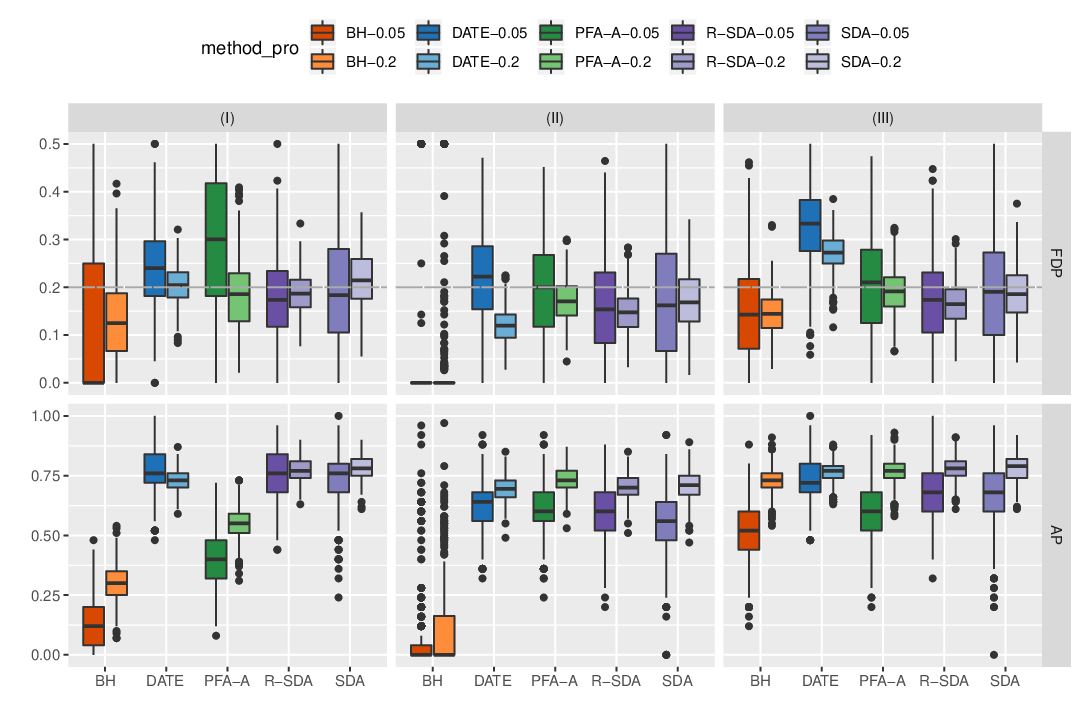
E.4 The impact of the number of tests and sample sizes
We also conduct experiments by altering the number of tests , while keeping . To make the AP comparable across , the signal is adjusted via with depending on the covariance structures. The results are summarized in the top half of Figure S7. We can see that all methods have more accurate control of FDR as increases, but the and DATE fail to control the FDR when is small. To investigate the impact on sample sizes with unknown covariance, we set , fix , and consider the normal error. The results are summarized in the bottom half of Figure S7. We can see that that our R-SDA method is able to control the FDR and close to the nominal level regardless of the choice of . Its superior performance relative to the other three methods is significant in some cases. Though all the methods exhibit steady AP pattern, the BH, PFA and DATE appear to need larger sample to achieve satisfactory FDR control than the R-SDA does. This again concurs with our theoretical result in Theorem 2 and demonstrates the advantage of using the nonparametric estimation of FDP in the SDA procedure.


E.5 List of selected genes by different methods
Table S1 reports the list of 19 most differentially expressed probe sets obtained by the methods R-SDA, BH, SS, PFA-A and DATE in the real-data example.
| R-SDA | BH | SS | PFA | DATE |
|---|---|---|---|---|
| 1635at | 1636gat | 39730at | 1636gat | 36502at |
| 39730at | 39730at | 39317at | 39730at | 38385at |
| 1636gat | 1635at | 37027at | 1635at | 40202at |
| 36502at | 1674at | 38052at | 1674at | 37403at |
| 37403at | 40504at | 1635at | 40202at | 38052at |
| 32134at | 40202at | 1636gat | 37403at | 33690at |
| 38052at | 37015at | 40202at | 32434at | 39317at |
| 36821at | 37027at | 34850at | 37014at | 40876at |
| 38385at | 32434at | 37403at | 32979at | 33440at |
| 37027at | 40167sat | 37024at | 1249at | 1674at |
| 1674at | 40480sat | 1249at | 38111at | 36908at |
| 41872at | 36591at | 36802at | 37015at | 33774at |
| 33440at | 33774at | 37025at | 37147at | 39730at |
| 32434at | 37403at | 32979at | 40504at | 41592at |
| 40876at | 37014at | 34870at | 33440at | 32134at |
| 40202at | 37363at | 36502at | 38112gat | 39070at |
| 39317at | 34472at | 33891at | 36502at | 37558at |
| 32562at | 32542at | 34800at | 31786at | 33304at |
| 34990at | 39329at | 36543at | 34850at | 34180at |