Delayed coincidence in electron-neutrino capture on gallium for neutrino spectroscopy
Abstract
This work explains a delayed-coincidence method to perform MeV-scale neutrino spectroscopy with electron-neutrino capture on gallium. An electron-neutrino possessing energy greater than 407.6 keV can be captured on gallium and produce a daughter germanium nucleus at its first excited state with a mean lifetime of 114 ns. The released electron and gammas before the first excited state of Ge can generate a prompt signal representing the solar neutrino energy and the gamma from the deexcitation of the first excited state, 175 keV, can give a delayed signal. The cross-section of this electron-neutrino capture process is evaluated and is comparable with electron-neutrino capture on chlorine. A possible implementation with a liquid scintillator is discussed to exploit the delayed coincidence. The detection scheme is more feasible than using 115In, etc., but need a larger target. The proposed method can be helpful for the MeV-scale solar neutrino spectroscopy and for solving the gallium anomaly.
I Introduction
The early works by J. Bahcall Joh and R. Davis Cleveland et al. 1998, and many results achieved later by other experiments such as GALLEX Hampel et al. 1999, GNO Altmann et al. 2005, SAGE Abdurashitov et al. 2002, SNO Aharmim et al. 2013, Super Kamiokande Abe et al. 2016, KamLAND Abe et al. 2011, and Borexino Agostini et al. 2019 mark the legend of modern studies of solar neutrino. The standard solar model and neutrino oscillations are the most noteworthy achievements.
However, several theoretical and experimental puzzles continue to exist. The “upturn” effect, which is the increase in solar electron-neutrino survival probability from matter dominant region to vacuum region, is still poorly constrained by experiments de Holanda and Smirnov 2004; Bonventre et al. 2013; Friedland et al. 2004; Maltoni and Smirnov 2016. The carbon-nitrogen-oxygen (CNO) fusion neutrinos from the Sun, which are dominant of the fueling processes of high-temperature massive stars, have not been observed Agostini et al. 201911 1 After the submission of this work, the Borexino collaboration reported a measurement of the CNO neutrino flux of at the ICHEP 2020 conference.. For the metal-element abundance prediction of the Sun, a conflict exists between the helioseismic prediction and the standard-solar-model assumption Haxton 2014; Serenelli et al. 2009a; Serenelli et al. 2011. Moreover, in the source tests with 51Cr and 37Ar at the GALLAX and SAGE experiments, the neutrino flux observations show a deficit from the predictions Hampel et al. 1998; Abdurashitov et al. 1999, known as “gallium anomaly”. Experimental and theoretical progress in the future is expected to address these issues.
Electron-neutrino capture on a nucleus,
| (1) |
provides a detection channel of the pure weak charged-current (CC) interaction for MeV-scale neutrino spectroscopy, in which the energies of the neutrino and the emitted electron simply differ by an energy threshold Bahcall 1964. Neutrino-electron scattering also provides a detection channel of the charged current together with the neutral-current interaction, but the energy of the recoiled electron is a complicated function of the neutrino energy and the electron emission angle, for example, as shown in Giunti and Kim 2007. Comparing these two types of detection channels, a large number of target electrons are easier to collect in water or an organic liquid scintillator, but the -nucleus capture is more convenient to extract the physics depending on the neutrino energy, such as the upturn effect and the structure of CNO neutrinos.
The SNO experiment measured the kinetic energy spectrum above 3.5 MeV Aharmim et al. 2013 using the CC process which has a reaction threshold 1.44 MeV. All the rest -nucleus capture measurements have only chemically detected the final state nuclei and no energy measurement of the emitted electrons is available so far. None of them has effectively addressed the upturn feature and CNO neutrinos.
The delayed-coincidence technique for -nucleus capture has been actively discussed for nuclei, such as 115In, 100Mo, 176Yb, 116Cd, etc. Raghavan 1976; Ejiri et al. 2000; Raghavan 1997; Zuber 2003 because it can greatly decrease the demand for the radioactive purity of the detection material and distinguish the signal from the background -electron scattering. The experimental efforts are still in progress, and facing a lot of technical challenges Yeh et al. 2007, for example, the high radioactivity of 115In.
II Delayed coincidence in capture on gallium
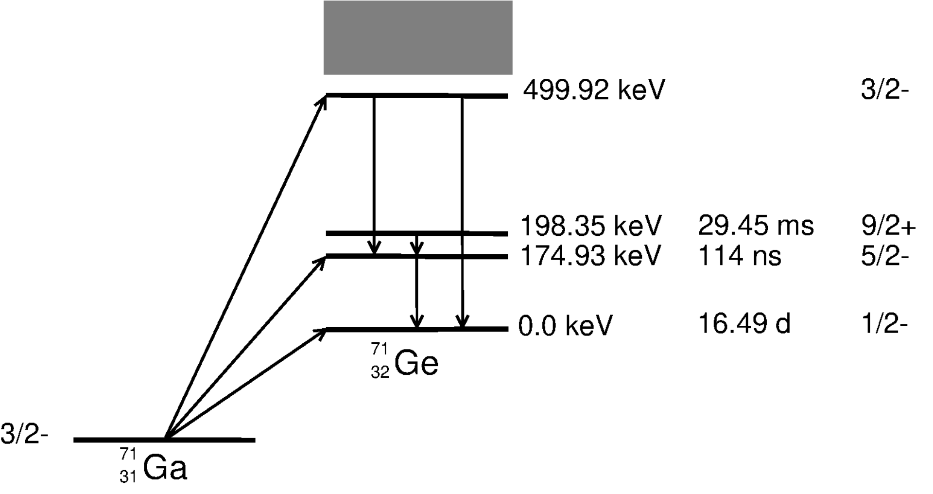
In this work, we propose a delayed-coincidence method to use gallium to perform a study on solar neutrino spectroscopy. An energy level plot of the Ga-Ge system is presented in Fig. for a few relevant states. The process is described in detail below,
| (2) |
which is followed by
| (3) |
Through the charge-current reaction an electron-neutrino is captured on and emits an electron and a nucleus at an excited state. The direct nucleus product can be the first excited state of at 175 keV (5/2-) or other higher levels, which can subsequently decay to the first excited state through one or a few gamma decays with certain probabilities. The first excited state has a mean lifetime of 114 ns Graves and Mitchell 1955; Morgenstern et al. 1968; Taff and Klinken 1978. The electron and deexcitation gammas in Eq. 1 form a prompt signal. The neutrino energy, , is the sum of the prompt energy, , and the reaction threshold ens; Bahcall 1997,
| (4) |
The deexcitation of the first excited state in Eq. 3 results in a delayed signal and coincidence. Note that there is a level at 198 keV with a lifetime of 29.45 ms and must be taken into consideration (Fig. 1). The gallium can be dissolved in a liquid scintillator and the delay-coincidence signals can be detected with a photomultiplier tube (PMT) array and a modern fast electronic readout system.
III Cross-section
The differential capture cross-sections of each energy level, , can be calculated with the approach described in Bahcall 1989; Bahcall 1978; Giunti et al. 2012; Barinov et al. 2018,
| (5) |
where s are the Gamow-Teller strengths for each level, was introduced in Bahcall 1989; Bahcall 1978 in which the ground state transition strength was considered, and are the energy and momentum of the electron in the unit of electron mass, respectively, is the fine-structure constant, and is the Fermi function with and , which can be calculated according to Bahcall 1989; Blatt and Weisskopf 1979. The values were measured through the charge-exchange reaction in Frekers et al. 2015 and are listed in Table 1. For a conservative cross-section estimation, we didn’t take the shell-model calculation result for B(GT) of the 5/2- level, which is five times larger Haxton 1998.
To evaluate the total cross section, , the incident neutrino energy spectrum , all the allowed excited energy levels, and their branching ratios to the first excited state, , are considered
| (6) |
where the energy integral region [, ] is limited by the of interest for detection and the contributions through the 198 keV level are excluded. The branching ratios of the excited states to the first excited state can be calculated based on the information given in ENSDF ens. However, only the data up to approximately 2 MeV are available for this estimation. Table 1 summarizes the branching fractions.
With Eq. 5 and 6 and the input in Table 1, the capture cross-sections of solar pp, 7Be, pep, and CNO neutrinos and 51Cr and 37Ar neutrinos are calculated and listed in Table 2 where the solar neutrino spectrum input is from Joh and the 51Cr and 37Ar spectrum input is from Abdurashitov et al. 1999.
| levels | (GT) | BR |
| MeV | ||
| 0 | 8.52(11) | 0 |
| 174.9 | 0.34(26) | 1 |
| 499.9 | 1.76(14) | 0.004777 |
| 708.2 | 0.11(5) | 0.04489 |
| 808.2 | 2.29(10) | 0.241717 |
| 1095.5 | 1.83(17) | 0.0725541 |
| 1298.7 | 1.33(8) | 0.0249493 |
| 1378.6 | 0.33(4) | 0.409911 |
| 1598.5 | 0.11(5) | 0.201239 |
| 1743.4 | 0.68(2) | 0.170329 |
| 1965 | 0.12(6) | 0 |
| MeV | |||
| pp | 0.42 MeV | 0 | |
| pep | 1.45 MeV | 8.2 | 8.2 |
| 7Be-380 | 0.38 MeV | 0 | 0 |
| 7Be-860 | 0.86 MeV | 1.96 | 1.96 |
| 13N | 1.19 MeV | 1.52 | 1.37 |
| 15O | 1.73 MeV | 3.87 | 3.79 |
| 17F | 1.74 MeV | 3.90 | 3.83 |
| 51Cr | 0.747 MeV | 1.49 | 1.49 |
| 51Cr | 0.752 MeV | 1.51 | 1.51 |
| 51Cr | 0.427 MeV | 0.51 | 0 |
| 51Cr | 0.432 MeV | 0.52 | 0 |
| 51Cr | all | 1.39 | 1.34 |
| 37Ar | 0.811 MeV | 1.74 | 1.74 |
| 37Ar | 0.813 MeV | 1.74 | 1.74 |
| 37Ar | all | 1.74 | 1.74 |
IV Gallium-loaded liquid scintillator detector
One measurement scheme is a Ga-loaded liquid scintillator. The Ga-loaded liquid scintillator is contained in a spherical transparent container. The scintillation and Cherenkov lights emitted by the prompt and delayed signals are detected by PMTs, and subsequently read out with fast electronics.
There are several applications to load different elements into an organic liquid scintillator. The Te-loaded liquid scintillator Biller 2015, In-loaded liquid scintillator Raghavan and the LENS Collaboration 2008, Gd-loaded liquid scintillator Yeh et al. 2007, and Li-loaded liquid scintillator Ashenfelter et al. 2018 are some examples. A method to load other elements into water-based liquid scintillators also exists Yeh et al. 2011.
The timing feature of the PMT and electronics is suitable for such a method. The rising time of the large diameter PMTs (8 inches) Ham is less than 10 ns and their transition time spread is 2-4 ns. Fast waveform digitizers can be found cae with a sampling rate of 1 Giga samples per second and no dead time.
The random coincident background from natural radioactivities is negligible for a 342 ns coincident window (3lifetime) according to the calculation method in Raghavan 1976; Ejiri et al. 2000.
The late pulse of the PMTs should be considered. Actual PMT time residual distributions in a large detector are presented by the SNO experiment (Fig. 5 of Aharmim et al. 2005 and Fig. 3 of Aharmim et al. 2007), where the late pulse rate is approximately 1% of the major pulse height per 0.33 ns from 10 to 80 ns because of the PMT’s, electronics and reflections, and only 0.2% per 0.33 ns after 80 ns. Considering a light yield of 500 photoelectrons (PE) per MeV in a liquid scintillator detector and a prompt 2 MeV signal, the number of PE for the prompt and delayed signals are 1000 and 88, respectively. After 80 ns, the number of PE for the late pulse in a 20 ns window is approximately 4, so that identifying the 175-keV delayed signal is not a concern.
V Requirement for CNO neutrinos
The requirement for the CNO neutrino detection will be discussed in this session. Both statistics and detector energy resolution are important for CNO neutrino detection and for separating each CNO component.
The statistics of the neutrino signals, , can be calculated with the neutrino flux as
| (7) |
where is the number of target nuclei, is the data-taking time, and is the survival probability. So the product of target Ga mass, , and data-taking time, , is the first key factor to consider. With the CNO neutrino flux prediction given in the low-metallicity solar model Serenelli et al. 2009b and the neutrino oscillation parameters Tanabashi et al. 2018, the event rates of 13N and 15O+17F are
| (8) | |||
| (9) |
where the mass is for natural gallium and the signals of 15O and 17F are treated together, because their spectra are indistinguishable and these conventions are used for the whole paper. We found that 52.9 kton year and 29.4 kton year are the thresholds to reach 10% precision for 13N and 15O+17F measurement, respectively.
A good energy resolution, , is also expected so the 13N and 15O+17F neutrinos can be distinguished from other solar neutrino components, i.e. the 7Be and pep neutrinos, and the feature can be seen in Fig. 2. The energy resolution is governed by the light yield, (number of photoelectrons, PE, per MeV) with .
To give a better understanding of the requirement, we simulated the solar neutrino signals according to the neutrino fluxes predicted by the low-metallicity solar model Serenelli et al. 2009b and a few detector configurations with different and . The simulated spectrum is then fitted with the known solar neutrino spectra and the fit result gives the expected uncertainty in determining the 13N and 15O+17F fluxes. An example can be seen in Fig. 2. Here the detection efficiency is assumed to be 100% and no other background is considered. More detail of the method can be found in Ref. Beacom et al. 2017. After scanning through several detector configurations, Tab. 3 gives a few promising results. In summary, assuming a 20-year data-taking time, a few kton of natural gallium is needed to measure the 13N and 15O+17F fluxes.
| 200 PE/MeV | 500 PE/MeV | ||
|---|---|---|---|
| 25 kton year | 13N | 0.37 | 0.25 |
| 15O+17F | 0.25 | 0.19 | |
| 50 kton year | 13N | 0.23 | 0.20 |
| 15O+17F | 0.18 | 0.14 | |
| 100 kton year | 13N | 0.17 | 0.13 |
| 15O+17F | 0.12 | 0.09 |
VI Requirement for 51Cr neutrinos
To study 51Cr neutrino capture cross-section, the number of 51Cr signal, N, is estimated as
| (10) |
where is the strength of the source, is the data-taking time, is the number density of 71Ga, and is the path length through Ga. We assume an intensive 51Cr source is placed in the center of a spherical detector and is the radius of the sensitive region with 100% detection efficiency. The source has a constant rate of 50 PBq similar to GALLEX and SAGE Hampel et al. 1998; Abdurashitov et al. 1999. The Ga-loaded liquid scintillator has a density of 1 g/cm3 and the natural Ga mass fraction is 10%. We must say the above assumptions are not realistic at all, but they will provide a useful estimation for the order of magnitude. The calculation shows
| (11) | |||
| (12) |
To get at least 100 signals, the product of the detector radius and data-taking time must be larger than 13 meter year, or equivalently the natural Ga mass times data-taking time larger than 0.97 kton year.
VII Discussion and conclusion
In this work we explained the delayed-coincidence method in capture on and evaluated the cross-sections below 2 MeV.
Naturally, gallium has only two stable isotopes and the natural abundance of is 39.9%. This overcomes the difficulty of intrinsic background in Raghavan 1976 and Ejiri et al. 2000. The coincident time of is the shortest among 115In, 100Mo, and 116Cd Zuber 2003 and is just over the limitation of PMT system. The delayed energy is higher than 176Yb Raghavan 1997 and is also higher than the endpoint of 14C, which is contained in organic detection material. Experimentally it is easier to implement.
The cross-section going through the first excited state of is 2%-3% of that going through the ground state and much smaller than 115In; however it is comparable with that of Bahcall 1989 which was used by R. Davis. If we take the B(BG) for the 5/2- level of shell-model prediction Haxton 1998, the cross-section is five times larger. This is the largest uncertainty and at this moment, we cannot exclude one or the other. The cross-section beyond 2 MeV can be measured using a neutrino source on a spallation neutron facility Bolozdynya et al. 2012; Chen and Wang 2016 with a known spectrum from the muon decay.
The application of loading Ga into a liquid scintillator is also discussed. The delayed signal is well detectable by a modern PMT-digitizer array. The background situation is promising except for some efficiency loss due to the late PMT pulses.
In the search of the CNO neutrinos, this method is clear of the unfolding complexity of the electron targets and can be useful for directly measuring the solar energy spectrum and extracting 13N and 15O+17F neutrinos separately.
For the gallium anomaly, the method could be interesting, because the considerable focus of the cause is on the neutrino capture cross-section prediction for the first excited state of Haxton 1998; Frekers et al. 2015; Giunti et al. 2012. This method will give an insight into the popular speculation on the systematic uncertainty of the first excited state of 71Ge.
To reach a 10% precision of 13N, 15O+17F, and 51Cr neutrinos, the need for natural Ga mass is at kton scale.
In summary, the delayed-coincidence in 71Ga(,)71Ge reaction involving the first excited state of 71Ge could be technically applicable for MeV neutrino spectroscopy. For the studies of gallium anomaly, upturn, and CNO neutrinos, it is an approach to consider.
Acknowledgement
This work is supported in part by the National Natural Science Foundation of China (Nos. 11620101004, 11475093, and 11235006), the Ministry of Science and Technology of China (No. 2018YFA0404102), the Key Laboratory of Particle & Radiation Imaging (Tsinghua University), and the CAS Center for Excellence in Particle Physics (CCEPP).
References
- (1) J. Bahcall home page: http://www.sns.ias.edu/˜jnb/.
- Cleveland et al. (1998) B. T. Cleveland et al., “Measurement of the solar electron neutrino flux with the Homestake chlorine detector,” Astrophys. J. 496, 505–526 (1998).
- Hampel et al. (1999) W. Hampel et al. (GALLEX), “GALLEX solar neutrino observations: Results for GALLEX IV,” Phys. Lett. B447, 127–133 (1999).
- Altmann et al. (2005) M. Altmann et al. (GNO), “Complete results for five years of GNO solar neutrino observations,” Phys. Lett. B616, 174–190 (2005).
- Abdurashitov et al. (2002) J. N. Abdurashitov et al. (SAGE), “Solar neutrino flux measurements by the Soviet-American Gallium Experiment (SAGE) for half the 22 year solar cycle,” J. Exp. Theor. Phys. 95, 181–193 (2002), [Zh. Eksp. Teor. Fiz.122,211(2002)].
- Aharmim et al. (2013) B. Aharmim et al. (SNO), “Combined Analysis of all Three Phases of Solar Neutrino Data from the Sudbury Neutrino Observatory,” Phys. Rev. C88, 025501 (2013).
- Abe et al. (2016) K. Abe et al. (Super-Kamiokande), “Solar Neutrino Measurements in Super-Kamiokande-IV,” Phys. Rev. D94, 052010 (2016).
- Abe et al. (2011) S. Abe et al. (KamLAND), “Measurement of the 8B Solar Neutrino Flux with the KamLAND Liquid Scintillator Detector,” Phys. Rev. C84, 035804 (2011).
- Agostini et al. (2019) M. Agostini et al. (Borexino), “First Simultaneous Precision Spectroscopy of , 7Be, and Solar Neutrinos with Borexino Phase-II,” Phys. Rev. D100, 082004 (2019).
- de Holanda and Smirnov (2004) P. C. de Holanda and A. Yu. Smirnov, “Homestake result, sterile neutrinos, and low energy solar neutrino experiments,” Phys. Rev. D 69, 113002 (2004).
- Bonventre et al. (2013) R. Bonventre et al., “Non-Standard Models, Solar Neutrinos, and Large ,” Phys. Rev. D88, 053010 (2013).
- Friedland et al. (2004) Alexander Friedland, Cecilia Lunardini, and Carlos Pena-Garay, “Solar neutrinos as probes of neutrino matter interactions,” Phys. Lett. B594, 347 (2004).
- Maltoni and Smirnov (2016) Michele Maltoni and Alexei Yu. Smirnov, “Solar neutrinos and neutrino physics,” Eur. Phys. J. A52, 87 (2016).
- Haxton (2014) Wick Haxton, “Neutrino physics: What makes the Sun shine,” Nature 512, 378–380 (2014).
- Serenelli et al. (2009a) Aldo Serenelli, Sarbani Basu, Jason W. Ferguson, and Martin Asplund, “New Solar Composition: The Problem With Solar Models Revisited,” Astrophys. J. 705, L123–L127 (2009a).
- Serenelli et al. (2011) Aldo M. Serenelli, W. C. Haxton, and Carlos Pena-Garay, “Solar models with accretion. I. Application to the solar abundance problem,” Astrophys. J. 743, 24 (2011).
- Hampel et al. (1998) W Hampel et al., “Final results of the neutrino source experiments in gallex,” Physics Letters B 420, 114 – 126 (1998).
- Abdurashitov et al. (1999) J. N. Abdurashitov et al. (The SAGE Collaboration), “Measurement of the response of a gallium metal solar neutrino experiment to neutrinos from a source,” Phys. Rev. C 59, 2246–2263 (1999).
- Bahcall (1964) John N. Bahcall, “Solar neutrino cross sections and nuclear beta decay,” Phys. Rev. 135, B137–B146 (1964).
- Giunti and Kim (2007) C. Giunti and C. W. Kim, Fundamentals of Neutrino Physics and Astrophysics (Oxford University Press, 2007).
- Raghavan (1976) R. S. Raghavan, “Inverse beta decay of 115-In to 115-Sn*: a new possibility for detecting solar neutrinos from the proton-proton reaction,” Phys. Rev. Lett. 37, 259–262 (1976).
- Ejiri et al. (2000) H. Ejiri, J. Engel, R. Hazama, P. Krastev, N. Kudomi, and R. G. H. Robertson, “Spectroscopy of double beta and inverse beta decays from Mo-100 for neutrinos,” Phys. Rev. Lett. 85, 2917–2920 (2000).
- Raghavan (1997) R. S. Raghavan, “New prospects for real time spectroscopy of low-energy electron neutrinos from the sun,” Phys. Rev. Lett. 78, 3618–3621 (1997).
- Zuber (2003) K. Zuber, “Spectroscopy of low energy solar neutrinos using CdTe detectors,” Phys. Lett. B571, 148–154 (2003).
- Yeh et al. (2007) M. Yeh, A. Garnov, and R.L. Hahn, “Gadolinium-loaded liquid scintillator for high-precision measurements of antineutrino oscillations and the mixing angle, ,” Nucl. Instrum. Meth. A 578, 329 – 339 (2007).
- Graves and Mitchell (1955) William E. Graves and Allan C. G. Mitchell, “Disintegration of ,” Phys. Rev. 97, 1033–1036 (1955).
- Morgenstern et al. (1968) J. Morgenstern, J.W. Schmidt, G. Flgge, and H. Schmidt, “The g factor of the 175 kev state in and hyperfine fields of in and ,” Physics Letters B 27, 370 – 372 (1968).
- Taff and Klinken (1978) L.M. Taff and J. Van Klinken, “Nuclear halflives observed with delayed coincident summing,” Nuclear Instruments and Methods 151, 189 – 199 (1978).
- (29) From ENSDF database as of Nov. 18, 2019. Version available at http://www.nndc.bnl.gov/ensarchivals/.
- Bahcall (1997) John N. Bahcall, “Gallium solar neutrino experiments: Absorption cross sections, neutrino spectra, and predicted event rates,” Phys. Rev. C 56, 3391–3409 (1997).
- Bahcall (1989) John N. Bahcall, Neutrino Astrophysics (Cambridge University Press, 1989).
- Bahcall (1978) John N. Bahcall, “Solar neutrino experiments,” Rev. Mod. Phys. 50, 881–903 (1978).
- Giunti et al. (2012) C. Giunti et al., “Update of Short-Baseline Electron Neutrino and Antineutrino Disappearance,” Phys. Rev. D86, 113014 (2012).
- Barinov et al. (2018) Vladislav Barinov, Bruce Cleveland, Vladimir Gavrin, Dmitry Gorbunov, and Tatiana Ibragimova, “Revised neutrino-gallium cross section and prospects of BEST in resolving the Gallium anomaly,” Phys. Rev. D97, 073001 (2018).
- Blatt and Weisskopf (1979) John M. Blatt and Victor F. Weisskopf, Theoretical nuclear physics (Springer-Verlag, 1979).
- Frekers et al. (2015) D. Frekers et al., “Precision evaluation of the solar neutrino capture rate from the charge-exchange reaction,” Phys. Rev. C 91, 034608 (2015).
- Haxton (1998) W. C. Haxton, “Cross-section uncertainties in the gallium neutrino source experiments,” Phys. Lett. B431, 110–118 (1998).
- Biller (2015) Steven Biller, “+ with tellurium,” Physics Procedia 61, 205 – 210 (2015), 13th International Conference on Topics in Astroparticle and Underground Physics, TAUP 2013.
- Raghavan and the LENS Collaboration (2008) R S Raghavan and the LENS Collaboration, “LENS, MiniLENS—status and outlook,” Journal of Physics: Conference Series 120, 052014 (2008).
- Ashenfelter et al. (2018) J. Ashenfelter et al. (PROSPECT), “Performance of a segmented 6Li-loaded liquid scintillator detector for the PROSPECT experiment,” JINST 13, P06023 (2018).
- Yeh et al. (2011) M. Yeh et al., “A new water-based liquid scintillator and potential applications,” Nucl. Instrum. Meth. A 660, 51 – 56 (2011).
- (42) Hamamatsu Photonics, see also the web link http://www.hamamatsu.com/.
- (43) CAEN, see also the web link https://www.caen.it/.
- Aharmim et al. (2005) B. Aharmim et al. (SNO), “Electron energy spectra, fluxes, and day-night asymmetries of B-8 solar neutrinos from measurements with NaCl dissolved in the heavy-water detector at the Sudbury Neutrino Observatory,” Phys. Rev. C72, 055502 (2005).
- Aharmim et al. (2007) B. Aharmim et al. (SNO), “Determination of the and total 8B solar neutrino fluxes with the Sudbury neutrino observatory phase I data set,” Phys. Rev. C75, 045502 (2007).
- Serenelli et al. (2009b) Aldo Serenelli, Sarbani Basu, Jason W. Ferguson, and Martin Asplund, “New Solar Composition: The Problem With Solar Models Revisited,” Astrophys. J. Lett. 705, L123 (2009b).
- Tanabashi et al. (2018) M. Tanabashi et al. (Particle Data Group), “Review of Particle Physics,” Phys. Rev. D98, 030001 (2018).
- Beacom et al. (2017) John F. Beacom et al. (Jinping), “Physics prospects of the Jinping neutrino experiment,” Chin. Phys. C 41, 023002 (2017), arXiv:1602.01733 [physics.ins-det] .
- Bolozdynya et al. (2012) A. Bolozdynya et al., “Opportunities for Neutrino Physics at the Spallation Neutron Source: A White Paper,” (2012) arXiv:1211.5199 [hep-ex] .
- Chen and Wang (2016) H. Chen and X. Wang, “China’s first pulsed neutron source,” Nature Materials 15, 689–691 (2016).
*