: Efficient Non-linear Pooling for RAM Constrained Inference
Abstract
Standard Convolutional Neural Networks (CNNs) designed for computer vision tasks tend to have large intermediate activation maps. These require large working memory and are thus unsuitable for deployment on resource-constrained devices typically used for inference on the edge. Aggressively downsampling the images via pooling or strided convolutions can address the problem but leads to a significant decrease in accuracy due to gross aggregation of the feature map by standard pooling operators. In this paper, we introduce , a novel pooling operator based on Recurrent Neural Networks (RNNs), that efficiently aggregates features over large patches of an image and rapidly downsamples activation maps. Empirical evaluation indicates that an layer can effectively replace multiple blocks in a variety of architectures such as MobileNets, DenseNet when applied to standard vision tasks like image classification and face detection. That is, can significantly decrease computational complexity and peak memory usage for inference while retaining comparable accuracy. We use with the standard S3FD [50] architecture to construct a face detection method that achieves state-of-the-art MAP for tiny ARM Cortex-M4 class microcontrollers with under KB of RAM. Code is released at https://github.com/Microsoft/EdgeML.
1 Introduction
Convolutional Neural Networks (CNNs) have become ubiquitous for computer vision tasks such as image classification and face detection. Steady progress has led to new CNN architectures that are increasingly accurate, but also require larger memory and more computation for inference. The increased inference complexity renders these models unsuitable for resource-constrained processors that are commonplace on the edge in IoT systems and battery-powered and privacy-centric devices.
To reduce inference complexity, several techniques like quantization [44], sparsification [9, 27], cheaper CNN blocks [37, 22], or neural architecture search [41] have been proposed to train CNN models with lower inference cost and model size while retaining accuracy. However, these models still require large working memory for inference. Memory tends to be the most constrained resource on low power devices as it occupies a large fraction of the device die and has high sustained power requirement [24]. Most low power ARM Cortex-M* microcontrollers have less than 256 KB RAM.
Typical CNNs have large intermediate activation maps, as well as many convolution layers, which put together require large amount of RAM for inference (see Proposition 1). A standard approach to reducing working memory is to use pooling operators or strided convolution to bring down size of the activation map. In fact, standard CNNs have multiple such layers. However, such pooling operators aggregate the underlying activation map in a simplistic manner, which can lead to a significant loss of accuracy. As a result, their use is limited to small receptive fields, typically no larger than , and they can not be used to aggressively reduce the activation map by aggregating larger receptive fields.

In this paper, we propose a novel pooling operator that uses Recurrent Neural Networks (RNNs) to perform a more refined aggregation over a large receptive field of the activation map without compromising on accuracy. can be applied to any tensor structured problem, but we focus on 2D images for ease of exposition. For images, uses RNNs to aggregate information along rows & columns in a given patch. has three parameters – patch size or receptive field, stride, and output dimension – to control its expressiveness and ability to downsample. The operator matches standard pooling operators syntactically, so can be used to replace them in convolutional networks.
allows rapid down-sampling of images and activation maps, eliminating the need for many memory-intensive intermediate layers. is most effective when used to replace multiple CNN blocks in the initial stages of the network where the activation map sizes are large, and hence, require the most memory and compute. There, a single layer of can down-sample by a factor of or . For example, applied to a image with patch-size 16, stride 8, and 32 output channels results in a activation map, which can be stored in about KB, and can be computed one patch at a time without significant memory cost. Replacing a few blocks using reduces peak memory requirement significantly for typical CNN architectures without much loss of accuracy.
Our experiments demonstrate that can be used as an effective replacement for multi-layered, expensive CNN blocks in a variety of architectures such as MobileNets, DenseNets, S3FD, and for varied tasks such as image classification and face detection. For example, in a 10-class image classification task, +MobileNetV2 reduces the peak memory requirement of MobileNetV2 by up to 10 and MAdds (MAdds refers to Multiply-Adds as in MobileNetV2 [37]) by about , while maintaining the same accuracy. Additionally, due to its general formulation, can replace pooling layers anywhere in the architecture. For example, it can replace the final average pool layer in MobileNetV2 and improve accuracy by .
Finally, we modify the S3FD [50] architecture with to construct an accurate face detection model which needs only 225 KB RAM – small enough to be deployed on a Cortex-M4 based device – and achieves 0.78 MAP on the medium category of the WIDER FACE dataset [47] using 80 fewer MAdds than EXTD [48] – a state-of-the-art resource-constrained face detection method.
In summary, we make the following contributions:
- •
A novel pooling operator that can rapidly down-sample input in a variety of standard CNN architectures, e.g., MobileNetV2, DenseNet121 while retaining the expressiveness.
- •
Demonstrate that can reduce working memory and compute requirements for image classification and Visual Wake Words significantly while retaining comparable accuracy.
- •
By combining with S3FD, we obtain a state-of-the-art face detection model for ARM Cortex-M4 class devices.
2 Related Work
Pooling: Max-pooling, average-pooling and strided convolution layers [29] are standard techniques for feature aggregation and for reducing spatial resolution in CNNs. Existing literature on rethinking pooling [51, 15, 10] focuses mainly on increasing accuracy and does not take compute/memory efficiency into consideration which is the primary focus of this paper.
Efficient CNN architectures: Most existing research on efficient CNN architectures aims at reducing model size and number of operations per inference. These methods include designing new architectures such as DenseNet [21], MobileNets [20, 37] or searching for them (ProxylessNAS [3], EfficientNets [41], SqueezeNAS [38]). These architectures do not primarily optimize for the peak working memory, which is a critical constraint on devices powered by tiny microcontrollers. Previous work on memory-optimized inference manipulates existing convolution operator by reordering computations [5, 28] or performing them in place [13]. However, most of these methods provide relatively small memory savings and are validated on low-resolution images like CIFAR-10 [25]. Channel pruning [17] is a method that tries to reduce memory requirement by pruning out multiple convolution kernels in every layer. While effective, channel/filter pruning does not tackle gradual spatial downsampling and thus is a complementary technique to .
Visual Wake Words: Visual cues (visual wake word) to “wake-up" AI-powered home assistant devices require real-time inference on relatively small devices. Chowdhery et al. 2019 proposed a Visual Wake Words dataset and a resource-constrained setting to evaluate various methods. Section 5.2 discusses the efficient based models and their performance for this task.
Face-detection on tiny devices: Recent work including EXTD [48], LFFD [18], FaceBoxes [49] and EagleEye [52] address the problem of accurate real-time face detection on resource-constrained devices. EXTD and LFFD are the most accurate but have high compute and memory requirements. On the other hand, EagleEye and FaceBoxes have lower inference complexity but also suffer from lower MAP scores. Face detection using is discussed in Section 5.3.
RNNs for Computer Vision: RNNs have been successful for sequential tasks but haven’t been extensively explored in the context of computer vision. An early work, ReNet [42], uses RNN based layer as a replacement for a convolution layer but does not aim at improving efficiency. contrasts with ReNet as follows:
- a.
ReNet is designed to replace a convolutional layer by capturing the global context and leaves the local context to be captured by flattening non-overlapping patches. , on the other hand, uses overlapping patches and strongly captures local features and relies on subsequent standard convolutions to capture the global context. Hence, and ReNet are complementary methods and can be combined.
- b.
Semantically, is a generalized pooling operator and can replace any pooling layer or strided convolution. However, ReNet does not correspond to any pooling abstraction, making it hard to combine with existing CNN models. For example, can modify S3FD architecture to achieve state-of-the-art real-time face detection with < 1 MB RAM while ReNet fails to fit in that context as a replacement layer since the receptive field of the output of ReNet layer varies across spatial positions.
- c.
ReNet can still be used as a rapid downsampling layer. Table 2 shows that outperforms ReNet with lower model size and fewer MAdds across datasets and architectures. E.g. ReNet+MobileNetV2 applied to ImageNet-1K is almost 4% less accurate than +MobileNetV2, despite the same working RAM requirement and more MAdds per inference.
Inside-Outside Net [2] uses a ReNet based layer for extracting context features in object detection while PiCANet [31] uses it as a global attention function for salient object detection. L-RNN [45] inserts multiple ReNet based layers but in a cascading fashion. See Appendix B for more discussion.
3 What is ?
Consider the output of an intermediate layer in a CNN of size , where and are the number of rows and columns and is the number of channels. A typical pooling layer (e.g. max or average) with stride would halve the number of rows and columns. So, reducing dimensions by a factor of would require two such blocks of convolutions and pooling. Our goal is to reduce the activation of size to, say, or smaller in a single layer while retaining the information necessary for the downstream task. We do so using an illustrated in Figure 1 that utilizes strided operators.
3.1 The Operator and the
An operator of size takes as input an activation patch of size corresponding to input channels, and uses a pair of RNNs – of hidden dimension and with hidden dimension – to sweep the patch horizontally and vertically to produce a summary of size .
Algorithm 1 describes the operator wich applies two parallel pipelines to a patch and concatenates their outputs. In the first, traverses each row and summarizes the patch horizontally (Line 16) and then trverses the outputs of (Lines 17-18) bi-directionally. In the second pipeline first traverses along columns to summarize the patch vertically (Line 20) and then (Lines 21-22) summarizes bi-directionally.
While it is possible to use GRU [4] or LSTM [19] for the two instances of RNN in , we use FastGRNN [26] for its compact size and fewer MAdds (see Appendix H).
An consists of a single operator strided over an input activation map and takes as input two more parameters: patch size and the stride length. Note that there are only two RNNs ( & ) in an operator, thus weights are shared for both the row-wise and column-wise passes () and all bi-directional passes () across every instance of in an .
3.2 Probing the Efficacy of
Capturing edges, orientations, and shapes: To demonstrate the capabilities of RNNs as spatial operators for vision tasks such as capturing edges, orientations, and shapes, we performed experiments on synthetic data. learns how to capture edges, orientations, and shapes as effectively as convolutional layers which reinforces the choice of RNNs as spatial operators. Appendix C.1 provides further details of these experiments.
4 How to use the ?
can be used to modify standard CNN architectures and reduce their working memory as well as computational requirements. Typically, such modifications involve replacing one or more stacks of convolutions and pooling layers of the “base” (original) architecture with an and retraining from scratch. We describe architecture modification strategies here and demonstrate their effectiveness through extensive experimentation in Section 5.
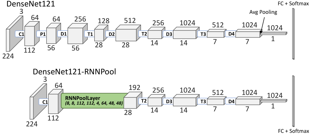
Replacement for a Sequence of Blocks: Consider the DenseNet121 [21] architecture in Figure 2. It consists of one convolutional layer, followed by repetitions of “Dense” (D), “Transition” (T) and “Pooling” (P) blocks which gradually reduce the size of the image while increasing the number of channels. Of all these layers, the first block following the initial convolutional layer (D1) requires the most working memory and compute as it works on large activation maps that are yet to be down-sampled. Further, the presence of 6 layers within each dense block makes it harder to work with small memory (see Proposition 1). This is also true of other architectures such as MobileNetV2, EfficientNet, and ResNet.
We can use an to rapidly down-sample the image size and bypass intermediate large spatial resolution activations. In DenseNet121, we can replace 4 blocks - P1, D1, T1, D2 - spanning 39 layers with a single to reduce the activation map from size to (see Figure 2). The replacement can be executed patch-by-patch without re-computation, thus reducing the need to store the entire activation map across the image. These two factors greatly reduce the working memory size as well as the number of computations. DenseNet121- achieves an accuracy of on ImageNet-10 (see Appendix A for dataset details) which is comparable to of the original DenseNet121 model.
A similar replacement of functional blocks with can be performed for MobileNetV2 as specified in Table 10 of Appendix F, and leads to a similar reduction in the size of the largest activation map while retaining accuracy. These results extend to other networks like EfficientNet, ResNet and GoogLeNet [40], where residual connection based functional blocks in the initial parts can be effectively replaced with the with improvements in working memory and compute, while retaining comparable accuracy. These results are listed in Table 1. Appendix H presents further ablation studies on and its base model.
Replacement for Pooling Layers: has the same input and output interface as any pooling operator and hence, can replace any standard pooling layer while providing more accurate aggregation. For example, DenseNet121- has three pooling layers one each in T2, T3, and the final average pool layer. Table 1 shows that, on ImageNet-10, DensetNet121- loses 0.6% accuracy compared to its base model. But, replacing all three remaining pooling layers in DenseNet121- with a results in almost the same accuracy as the base DenseNet121 but with about 2 and 4 lower compute and RAM requirement respectively. We can further drop 14 dense layers in D3 and 10 layers in D4 to bring down MAdds and RAM requirement to 0.79G MAdds and 0.43 MB, respectively, while still ensuring accuracy.
Replacement in Face Detection models: As in the above architectures, we can use to rapidly down-sample the image by a factor of in the early phase of an S3FD face detector [50]. The resulting set of architectures (with different parameters) are described in Appendix F.2. For example, the -Face-Quant model has a state-of-the-art MAP for methods that are constrained to at most 256 KB of working RAM (Table 4).
| Model | Base | |||||||||
|---|---|---|---|---|---|---|---|---|---|---|
| Accuracy (%) | Parameters | Memory Optimised | Standard Calculation [6, 37] | |||||||
| Peak RAM | MAdds | Peak RAM | MAdds | Accuracy (%) | Parameters | Peak RAM | MAdds | |||
| MobileNetV2 | 94.20 | 2.20M | 0.38 MB | 1.00G | 2.29 MB | 0.30G | 94.40 | 2.00M | 0.24 MB | 0.23G |
| EfficientNet-B0 | 96.00 | 4.03M | 0.40 MB | 1.09G | 2.29 MB | 0.39G | 96.40 | 3.90M | 0.25 MB | 0.33G |
| ResNet18 | 94.80 | 11.20M | 0.38 MB | 21.58G | 3.06 MB | 1.80G | 94.40 | 10.60M | 0.38 MB | 0.95G |
| DenseNet121 | 95.40 | 6.96M | 1.53 MB | 24.41G | 3.06 MB | 2.83G | 94.80 | 5.60M | 0.77 MB | 1.04G |
| GoogLeNet | 96.00 | 9.96M | 1.63 MB | 3.32G | 3.06 MB | 1.57G | 95.60 | 9.35M | 0.78 MB | 0.81G |
Inference memory requirements: Computing exact memory and compute requirement of a large CNN model is challenging as the execution order of activations in various layers can be re-organized to trade-off memory and compute. For example, in the memory-optimized column of Table 1 we present the compute usage of a variety of baseline architectures when their execution order (EO) is restricted to using no more memory than the corresponding based architecture. That is, we identify the memory bottleneck layers in various architectures whose activation map size is almost same as that of the corresponding -based model. We then compute every voxel of this layer by re-computing the required set of convolutions, without storing them. CNNs, in general, have significant compute requirement and such re-compute intensive optimizations make the architecture infeasible even for large devices, e.g. DenseNet121 requires 24.41G MAdds in this scheme (Table 1).
A standard approach is to restrict execution orders that do not require any re-computation of intermediate activation maps. A straightforward and standard EO is the one where the computation is executed layer-by-layer [6, 37]. The memory requirement of such a scheme would correspond to the largest activation map in the architecture, except the output of 1x1 convolution layers which can be computed on the fly. This approach mimics the memory requirement of existing platforms like TF-lite [11] and is proposed as a standard benchmark for comparing resource-constrained inference methods [6]. Following this prior convention, we list the inference complexity for various architectures under the compute-optimized columns in Table 1, unless the operation is easy to compute on the fly like 1x1 convolution or patch-by-patch computation of . Appendix E.2 provides more details about these calculations.
The above scheme is easy to implement and allows an inference pipeline that is more modular and easy to debug and could allow faster inference on neural network accelerators [23]. But, in principle, one can design execution orders (EO) that do not re-compute any intermediate layers, but are still not required to store entire activation maps, especially the largest ones. So, a rigorous quantification of the memory requirement of a model (without any re-compute) needs to show that any valid execution order requires a certain amount of working memory at some point in its execution, and also demonstrate a valid EO with the same memory requirement as a matching upper bound. We achieve this with the following proposition, whose proof and corollaries are in Appendix D.
Proposition 1
Consider an -layer () convolutional network with a final layer of size . Suppose the for each node in the output layer, the size of receptive field in intermediate layer is and that this layer has channels and stride . Any serial execution order of this network that disallows re-computation requires at least memory for nodes in the intermediate layers.
The above proposition shows that for a CNN with receptive field at the -th layer, the memory requirement scales linearly with the height/width of the activation map and with the number of layers. As networks like MobileNetV2 or DenseNet have blocks with a significant number of convolution layers and large receptive field, this proposition implies that it is not possible to significantly reduce the memory requirement over the standard layer-by-layer approach. For example, our un-optimized calculations for architectures still give us x reduction in peak RAM usage when compared to the minimum RAM requirement of the corresponding base architecture (see Appendix E.1). Further, similar optimization can be applied to based architectures, so the relative reduction in memory by does not change significantly. The implications of the above proposition, i.e., the peak memory of various networks without re-compute is calculated in Appendix E.1.
| Method | ImageNet-10 | Visual Wake Words | |||||||||
|---|---|---|---|---|---|---|---|---|---|---|---|
| MobileNetV2 | DenseNet121 | MobileNetV2-0.35 | |||||||||
| Accuracy (%) | MAdds | Parameters | Accuracy (%) | MAdds | Parameters | Accuracy (%) | MAdds | Parameters | |||
| Base Network | 94.20 | 0.300G | 2.2M | 95.40 | 2.83G | 6.96M | 90.20 | 53.2M | 296K | ||
| Last layer | 95.00 | 0.334G | 2.9M | 95.40 | 3.05G | 7.41M | 91.14 | 53.4M | 300K | ||
| Average Pooling | 90.80 | 0.200G | 2.0M | 92.80 | 0.71G | 5.59M | 86.85 | 31.9M | 255K | ||
| Max Pooling | 92.80 | 0.200G | 2.0M | 93.40 | 0.71G | 5.59M | 86.92 | 31.9M | 255K | ||
| Strided Convolution | 93.00 | 0.258G | 2.1M | 93.80 | 1.33G | 6.38M | 88.08 | 39.2M | 264K | ||
| ReNet | 92.20 | 0.296G | 2.3M | 93.00 | 1.35G | 6.41M | 88.10 | 46.4M | 277K | ||
| 94.40 | 0.226G | 2.0M | 94.80 | 1.04G | 5.60M | 89.57 | 37.7M | 255K | |||
|
95.60 | 0.260G | 2.7M | 95.00 | 1.26G | 6.06M | 89.65 | 37.9M | 259K | ||
5 Evaluation of on Vision Tasks
We present empirical evidence that operator is compatible with popular CNN architectures for vision tasks, and can push the envelope of compute/memory usage vs accuracy curve. Further, we show that combined with MobileNetV2 [37] generates accurate models for Visual wake words and face detection problems that can be deployed on tiny Cortex-M4 microcontrollers. See Appendix G for more details about model training and hyperparameters used for the experiments.
5.1 for Image Classification
We first focus on ImageNet-10, a 10 class subset of ImageNet-1K [7] where the classes correspond to the categories in CIFAR-10 [25]. We study this dataset because in several realistic tiny devices scenario, like intrusion detection, we are interested in identifying the presence/absence of a few, rather than 1000, classes of objects. The dataset is divided into 1300 images for training and 50 for validation per class. More details and rationale about the dataset can be found in the Appendix A.
Table 2 compares against other standard pooling operators as used in MobileNetV2 and DenseNet121 base networks (see Appendix F.1 for description of the architecture). It shows that with the same memory usage, is up to % more accurate than the standard pooling operators. While standard pooling operators are cheaper than , the overall compute requirement of based architectures is similar to pooling based architectures. Furthermore, replacing the last average pooling layer in the base network with further increases accuracy, thus demonstrating the flexibility of . Table 2 also contrasts with ReNet [42] as a downsampling layer. We observe that is a much better alternative for downsampling layers in terms of accuracy (better by up to 2%), model size, and MAdds for the same amount of working memory.
Next, we study the compatibility of with different architectures. Table 1 shows that based architectures maintain the accuracy of base models while significantly decreasing memory and compute requirement. See Section 4 and Appendix E for a discussion on the calculation of memory and compute requirements of different models.
| Method | Peak RAM | Parameters | MAdds | Accuracy (%) |
|---|---|---|---|---|
| MobileNetV1 | 3.06MB | 4.2M | 569M | 69.52 |
| MobileNetV1-ReNet | 0.77MB | 4.2M | 487M | 66.90 |
| MobileNetV1- | 0.77MB | 4.1M | 417M | 69.39 |
| MobileNetV2 | 2.29MB | 3.4M | 300M | 71.81 |
| MobileNetV2-ReNet | 0.24MB | 3.6M | 296M | 66.72 |
| MobileNetV2- | 0.24MB | 3.2M | 226M | 70.14 |
Finally, Table 3 presents results on the complete ImageNet-1K [7] dataset with MobileNetV1 and MobileNetV2 as the base architectures. ReNet and based models are constructed in a manner similar to the models in Table 1. See Table 10 for the complete specification of the MobileNetV2+ model. MobileNetV1+ model is constructed similarly with . Consistent with the results on ImageNet-10, retains almost same accuracy as the base models while decreasing memory usage significantly. Furthermore, based models are also % more accurate than ReNet based models. In this work, we focus on state-of-the-art resource-constrained models that do not require neural architecture search (NAS); we leave extension of for NAS based architectures like EfficientNets [41] for future work.
5.2 for Visual Wake Words

The Visual Wake Words challenge [6] presents a relevant use case for computer vision on tiny microcontrollers. It requires detecting the presence of a human in the frame with very little resources — no more than 250 KB peak RAM usage and model size, and no more than 60M MAdds/image. The existing state-of-the-art method [6] is MobileNetV2- with 8 channels for the first convolution and 320 channels for the last convolution layer. We use this as our baseline and replace convolutions with an . After training a floating-point model with the best validation accuracy, we perform per-channel quantization to obtain 8-bit integer weights and activations.
Table 2 compares the accuracy of the baseline and new architectures on this task. Replacing the last average pool layer with increases the accuracy by 1%. Inserting both at the beginning of the network and at the end provides a model whose accuracy is within % of the baseline but with far smaller memory requirement (250 33.68 KB), model size, and MAdds. Peak memory usage is calculated using the same convention as [6].
Further, we sweep across input image resolutions of {96, 128, 160, 192, 224} to trade-off between accuracy and efficiency. Figure 3 shows that models are significantly cheaper during inference in terms of compute and memory while offering the same accuracy as the baselines. For example, peak memory usage of MobileNetV2-0.35 with the lowest resolution images is 40 KB, while our model requires only 34 KB RAM despite using the highest resolution image and providing 4% higher accuracy. Note that ProxylessNAS [14] was the winner of the Visual Wake Words challenge. We report it’s accuracy on the final network provided by the authors. To be consistent, we train the model only on the training data provided, instead of pretraining with ImageNet-1K used by ProxylessNAS in the wake word challenge.
5.3 for Face Detection
| Method | Peak RAM | Parameters | MAdds | MAP | MAP for 3 faces | ||||
|---|---|---|---|---|---|---|---|---|---|
| Easy | Medium | Hard | Easy | Medium | Hard | ||||
| EXTD | 18.75 MB | 0.07M | 8.49G | 0.90 | 0.88 | 0.82 | 0.93 | 0.93 | 0.91 |
| LFFD | 18.75 MB | 2.15M | 9.25G | 0.91 | 0.88 | 0.77 | 0.83 | 0.83 | 0.82 |
| -- | 6.44 MB | 1.52M | 1.80G | 0.92 | 0.89 | 0.70 | 0.95 | 0.94 | 0.92 |
| FaceBoxes | 1.76 MB | 1.01M | 2.84G | 0.84 | 0.77 | 0.39 | - | - | - |
| -- | 1.76 MB | 1.12M | 1.18G | 0.87 | 0.84 | 0.67 | 0.91 | 0.90 | 0.88 |
| EagleEye | 1.17 MB | 0.23M | 0.08G | 0.74 | 0.70 | 0.44 | 0.79 | 0.78 | 0.75 |
| -- | 1.17 MB | 0.06M | 0.10G | 0.77 | 0.75 | 0.53 | 0.81 | 0.79 | 0.77 |
| -- | 225 KB | 0.07M | 0.12G | 0.80 | 0.78 | 0.53 | 0.84 | 0.83 | 0.81 |
We experiment with multiple architectures we call -Face-* for face detection suggested in Section 4 and described in greater detail in Appendix F.2. We train and validate these architectures with the WIDER FACE dataset [47]. Versions Quant, A, B, and C of the -Face use of hidden dimensions 4, 4, 6 and 16, respectively.
Table 4 compares validation Mean Average Precision (MAP) for easy, medium, and hard subsets. MAP is a standard metric for face detection and measures the mean area under the precision-recall curve. We report MAP scores for baselines based on the official open-source code or pre-trained models. For Eagle-Eye [52], we re-implemented the method as the source code was not available. For EXTD [48], we report MAdds of the EXTD-32 version - the computationally cheapest. EXTD and LFFD [18] are accurate but are computationally expensive. In contrast, -Face-C achieves better MAP in the easy and medium subsets despite using less compute and less RAM.
FaceBoxes [49] and Eagle-Eye reduce MAdds and peak memory usage by aggressively down-sampling the image or by decreasing the number of channels leading to inaccurate models. In contrast, -Face-A and -Face-B achieve significantly higher MAPs than these methods while still ensuring smaller MAdds and peak RAM usage. We also compare MAP scores for images that have 3 faces, which is a more realistic face-detection setting for tiny devices. Here also, -Face-C is more accurate than all the baselines. Finally, -Face-Quant uses byte quantization to reduce the model size so it can be deployed on Cortex-M4 devices which typically have KB RAM, while still having MAP accuracy on images with faces. See Appendix I for a qualitative evaluation of our method against the baselines.
5.4 based Model for ARM Cortex-M4 Microcontrollers
Finally, we develop a face detection model for conference/class room settings that can be deployed on ARM Cortex-M4 class devices. To this end, we develop a more compact version of the face detection model, -Face-M4 (Table 15 in Appendix F.2), which has only 4 MBConv blocks. For further reduction in MAdds and model-size, we train the parameters to be sparse. That is, matrix of is 50% non-zeros while the rest of the matrices in are 30% non-zeros.
To not overshoot RAM for storing input image, we use 3202401 monochrome images for training and testing. For evaluation, we first train on the WIDER FACE dataset and then fine-tune on the SCUT-HEAD dataset [35] which consists of images in conference/class rooms. We then use the SeeDot [12] compiler to quantize our model to 8 bits and generate C code for deployment. Table 5 compares the resource requirements and MAP on the SCUT-HEAD validation set (random 80%-20% split) of -Face-M4 against a similarly trained MobileNetV2-SSDLite model which is a state-of-the-art architecture for low-cost detection.
| Model | MAP | Peak RAM | MAdds | Model Size |
|---|---|---|---|---|
| MobileNetV2-SSDLite | 0.63 | 3.51 MB | 540M | 11.32 MB |
| -Face-M4 | 0.58 | 188 KB | 70M | 160 KB |
Note that MobileNetV2-SSDLite cannot be deployed on a Cortex-M4 device even with 8-bit quantization as the peak RAM requirement is much more than the 256 KB limit of the device. -Face-M4 model processes a single image in 10.45 seconds on an ARM Cortex-M4 microcontroller based STM32F439-M4 device clocked at 168 MHz.
6 Conclusions
In this paper, we proposed , an efficient RNN-based pooling operator that can be used to rapidly downsample activation map sizes thus significantly reduce inference-time memory and compute requirements for a variety of standard CNNs. Due to syntax level similarity with pooling layers, we can use in most existing CNN based architectures. These replacements retain accuracy for tasks like image classification and visual wake words. Our S3FD based model for face detection provided accurate models that can be deployed on tiny Cortex-M4 microcontrollers. Finally, we showed with Proposition 1 that calculations of minimum memory requirement for standard architectures can be made rigorous and demonstrate that despite such optimizations of standard CNNs, based models can be significantly more efficient in terms of inference-time working memory. Using neural architecture search for based models to further reduce inference cost is an immediate and interesting direction.
Broader Impact
Pros: ML models are compute-intensive and are typically served on power-intensive cloud hardware with a large resource footprint that adds to the global energy footprint. Our models can help reduce this footprint by (a) allowing low power edge sensors with small memory to analyze images and admit only interesting images for cloud inference, and (b) reducing the inference complexity of the cloud models themselves. Further, edge-first inference enabled by our work can reduce reliance on networks and also help provide privacy guarantees to end-user. Furthermore, vision models on tiny edge devices enables accessible technologies, e.g., Seeing AI [33] for people with visual impairment.
Cons: While our intentions are to enable socially valuable use cases, this technology can enable cheap, low-latency and low-power tracking systems that could enable intrusive surveillance by malicious actors. Similarly, abuse of technology in certain wearables is also possible.
Again, we emphasize that it depends on the user to see the adaptation to either of these scenarios.
Acknowledgements
We are grateful to Shikhar Jaiswal and Aayan Kumar for their assistance in the deployment of models on Cortex-M4 devices. We also thank Sahil Bhatia, Ali Farhadi, Sachin Goyal, Max Horton, Sham Kakade and Ajay Manchepalli for helpful discussions and feedback. Aditya Kusupati did a part of this work during his research fellowship at Microsoft Research India.
References
- Acuna et al. [2018] D. Acuna, H. Ling, A. Kar, and S. Fidler. Efficient interactive annotation of segmentation datasets with polygon-rnn++. In The IEEE conference on Computer Vision and Pattern Recognition, pages 859–868, 2018.
- Bell et al. [2016] S. Bell, C. Lawrence Zitnick, K. Bala, and R. Girshick. Inside-outside net: Detecting objects in context with skip pooling and recurrent neural networks. In The IEEE Conference on Computer Vision and Pattern Recognition, June 2016.
- Cai et al. [2018] H. Cai, L. Zhu, and S. Han. ProxylessNAS: Direct neural architecture search on target task and hardware. arXiv preprint arXiv:1812.00332, 2018.
- Cho et al. [2014] K. Cho, B. Van Merriënboer, C. Gulcehre, D. Bahdanau, F. Bougares, H. Schwenk, and Y. Bengio. Learning phrase representations using rnn encoder-decoder for statistical machine translation. arXiv preprint arXiv:1406.1078, 2014.
- Cho and Brand [2017] M. Cho and D. Brand. Mec: memory-efficient convolution for deep neural network. In International Conference on Machine Learning, pages 815–824. JMLR. org, 2017.
- Chowdhery et al. [2019] A. Chowdhery, P. Warden, J. Shlens, A. Howard, and R. Rhodes. Visual wake words dataset. arXiv preprint arXiv:1906.05721, 2019.
- Deng et al. [2009] J. Deng, W. Dong, R. Socher, L.-J. Li, K. Li, and L. Fei-Fei. Imagenet: A large-scale hierarchical image database. In The IEEE conference on Computer Vision and Pattern Recognition, pages 248–255. Ieee, 2009.
- [8] D. K. Dennis, Y. Gaurkar, S. Gopinath, S. Goyal, C. Gupta, M. Jain, S. Jaiswal, A. Kumar, A. Kusupati, C. Lovett, S. G. Patil, O. Saha, and H. V. Simhadri. EdgeML: Machine Learning for resource-constrained edge devices. URL https://github.com/Microsoft/EdgeML.
- Gale et al. [2019] T. Gale, E. Elsen, and S. Hooker. The state of sparsity in deep neural networks. arXiv preprint arXiv:1902.09574, 2019.
- Gong et al. [2014] Y. Gong, L. Wang, R. Guo, and S. Lazebnik. Multi-scale orderless pooling of deep convolutional activation features. In European Conference on Computer Vision, pages 392–407. Springer, 2014.
- [11] Google. ML for mobile and edge devices - tensorflow lite. URL https://www.tensorflow.org/lite.
- Gopinath et al. [2019] S. Gopinath, N. Ghanathe, V. Seshadri, and R. Sharma. Compiling kb-sized machine learning models to tiny iot devices. In ACM SIGPLAN Conference on Programming Language Design and Implementation, pages 79–95, 2019.
- Gural and Murmann [2019] A. Gural and B. Murmann. Memory-optimal direct convolutions for maximizing classification accuracy in embedded applications. In International Conference on Machine Learning, pages 2515–2524, 2019.
- [14] S. Han, J. Lin, K. Wang, T. Wang, and Z. Wu. Solution to Visual Wakeup Words Challenge’19 (first place). URL https://github.com/mit-han-lab/VWW.
- He et al. [2015] K. He, X. Zhang, S. Ren, and J. Sun. Spatial pyramid pooling in deep convolutional networks for visual recognition. The IEEE transactions on Pattern Analysis and Machine Intelligence, 37(9):1904–1916, 2015.
- He et al. [2016] K. He, X. Zhang, S. Ren, and J. Sun. Deep residual learning for image recognition. In The IEEE conference on Computer Vision and Pattern Recognition, pages 770–778, 2016.
- He et al. [2017] Y. He, X. Zhang, and J. Sun. Channel pruning for accelerating very deep neural networks. In The IEEE International Conference on Computer Vision, pages 1389–1397, 2017.
- He et al. [2019] Y. He, D. Xu, L. Wu, M. Jian, S. Xiang, and C. Pan. LFFD: A light and fast face detector for edge devices. arXiv preprint arXiv:1904.10633, 2019.
- Hochreiter and Schmidhuber [1997] S. Hochreiter and J. Schmidhuber. Long short-term memory. Neural computation, 9(8):1735–1780, 1997.
- Howard et al. [2017] A. G. Howard, M. Zhu, B. Chen, D. Kalenichenko, W. Wang, T. Weyand, M. Andreetto, and H. Adam. Mobilenets: Efficient convolutional neural networks for mobile vision applications. arXiv preprint arXiv:1704.04861, 2017.
- Huang et al. [2017] G. Huang, Z. Liu, L. Van Der Maaten, and K. Q. Weinberger. Densely connected convolutional networks. In The IEEE conference on Computer Vision and Pattern Recognition, pages 4700–4708, 2017.
- Iandola et al. [2016] F. N. Iandola, S. Han, M. W. Moskewicz, K. Ashraf, W. J. Dally, and K. Keutzer. Squeezenet: Alexnet-level accuracy with 50x fewer parameters and< 0.5 mb model size. arXiv preprint arXiv:1602.07360, 2016.
- Jouppi et al. [2017] N. P. Jouppi, C. Young, N. Patil, D. Patterson, G. Agrawal, R. Bajwa, S. Bates, S. Bhatia, N. Boden, A. Borchers, et al. In-datacenter performance analysis of a tensor processing unit. In International Symposium on Computer Architecture, pages 1–12, 2017.
- Kim et al. [2017] D. Kim, J.-Y. Choi, and J.-E. Hong. Evaluating energy efficiency of internet of things software architecture based on reusable software components. International Journal of Distributed Sensor Networks, 13(1):1550147716682738, 2017.
- Krizhevsky et al. [2009] A. Krizhevsky, G. Hinton, et al. Learning multiple layers of features from tiny images. 2009.
- Kusupati et al. [2018] A. Kusupati, M. Singh, K. Bhatia, A. Kumar, P. Jain, and M. Varma. FastGRNN: A fast, accurate, stable and tiny kilobyte sized gated recurrent neural network. In Advances in Neural Information Processing Systems, pages 9017–9028, 2018.
- Kusupati et al. [2020] A. Kusupati, V. Ramanujan, R. Somani, M. Wortsman, P. Jain, S. Kakade, and A. Farhadi. Soft threshold weight reparameterization for learnable sparsity. In International Conference on Machine Learning, 2020.
- Lai et al. [2018] L. Lai, N. Suda, and V. Chandra. Cmsis-nn: Efficient neural network kernels for arm cortex-m cpus. arXiv preprint arXiv:1801.06601, 2018.
- LeCun et al. [2015] Y. LeCun, Y. Bengio, and G. Hinton. Deep learning. nature, 521(7553):436–444, 2015.
- Lin et al. [2014] T.-Y. Lin, M. Maire, S. Belongie, J. Hays, P. Perona, D. Ramanan, P. Dollár, and C. L. Zitnick. Microsoft coco: Common objects in context. In European Conference on Computer Vision, pages 740–755. Springer, 2014.
- Liu et al. [2018] N. Liu, J. Han, and M.-H. Yang. Picanet: Learning pixel-wise contextual attention for saliency detection. In The IEEE Conference on Computer Vision and Pattern Recognition, June 2018.
- Mead [1992] A. Mead. Review of the development of multidimensional scaling methods. Journal of the Royal Statistical Society: Series D (The Statistician), 41(1):27–39, 1992.
- [33] Microsoft. Seeing AI. URL https://www.microsoft.com/en-us/ai/seeing-ai.
- Paszke et al. [2019] A. Paszke, S. Gross, F. Massa, A. Lerer, J. Bradbury, G. Chanan, T. Killeen, Z. Lin, N. Gimelshein, L. Antiga, et al. Pytorch: An imperative style, high-performance deep learning library. In Advances in Neural Information Processing Systems, pages 8024–8035, 2019.
- Peng et al. [2018] D. Peng, Z. Sun, Z. Chen, Z. Cai, L. Xie, and L. Jin. Detecting heads using feature refine net and cascaded multi-scale architecture. arXiv preprint arXiv:1803.09256, 2018.
- Russakovsky et al. [2015] O. Russakovsky, J. Deng, H. Su, J. Krause, S. Satheesh, S. Ma, Z. Huang, A. Karpathy, A. Khosla, M. Bernstein, et al. Imagenet large scale visual recognition challenge. International Journal of Computer Vision, 115(3):211–252, 2015.
- Sandler et al. [2018] M. Sandler, A. Howard, M. Zhu, A. Zhmoginov, and L.-C. Chen. Mobilenetv2: Inverted residuals and linear bottlenecks. In The IEEE conference on Computer Vision and Pattern Recognition, pages 4510–4520, 2018.
- Shaw et al. [2019] A. Shaw, D. Hunter, F. Iandola, and S. Sidhu. SqueezeNAS: Fast neural architecture search for faster semantic segmentation. In ICCV Neural Architects Workshop, 2019.
- Sutskever et al. [2013] I. Sutskever, J. Martens, G. Dahl, and G. Hinton. On the importance of initialization and momentum in deep learning. In International Conference on Machine Learning, pages 1139–1147, 2013.
- Szegedy et al. [2015] C. Szegedy, W. Liu, Y. Jia, P. Sermanet, S. Reed, D. Anguelov, D. Erhan, V. Vanhoucke, and A. Rabinovich. Going deeper with convolutions. In The IEEE conference on Computer Vision and Pattern Recognition, pages 1–9, 2015.
- Tan and Le [2019] M. Tan and Q. Le. EfficientNet: Rethinking model scaling for convolutional neural networks. In International Conference on Machine Learning, pages 6105–6114, 2019.
- Visin et al. [2015] F. Visin, K. Kastner, K. Cho, M. Matteucci, A. Courville, and Y. Bengio. Renet: A recurrent neural network based alternative to convolutional networks. arXiv preprint arXiv:1505.00393, 2015.
- Wang et al. [2016] J. Wang, Y. Yang, J. Mao, Z. Huang, C. Huang, and W. Xu. CNN-RNN: A unified framework for multi-label image classification. In The IEEE conference on Computer Vision and Pattern Recognition, pages 2285–2294, 2016.
- Wang et al. [2019] K. Wang, Z. Liu, Y. Lin, J. Lin, and S. Han. Haq: Hardware-aware automated quantization with mixed precision. In The IEEE conference on Computer Vision and Pattern Recognition, pages 8612–8620, 2019.
- Xie et al. [2016] W. Xie, A. Noble, and A. Zisserman. Layer recurrent neural networks. 2016.
- Xingjian et al. [2015] S. Xingjian, Z. Chen, H. Wang, D.-Y. Yeung, W.-K. Wong, and W.-c. Woo. Convolutional LSTM network: A machine learning approach for precipitation nowcasting. In Advances in Neural Information Processing Systems, pages 802–810, 2015.
- Yang et al. [2016] S. Yang, P. Luo, C.-C. Loy, and X. Tang. Wider face: A face detection benchmark. In The IEEE conference on Computer Vision and Pattern Recognition, pages 5525–5533, 2016.
- Yoo et al. [2019] Y. Yoo, D. Han, and S. Yun. EXTD: Extremely tiny face detector via iterative filter reuse. arXiv preprint arXiv:1906.06579, 2019.
- Zhang et al. [2017a] S. Zhang, X. Zhu, Z. Lei, H. Shi, X. Wang, and S. Z. Li. Faceboxes: A CPU real-time face detector with high accuracy. In The IEEE International Joint Conference on Biometrics, pages 1–9. IEEE, 2017a.
- Zhang et al. [2017b] S. Zhang, X. Zhu, Z. Lei, H. Shi, X. Wang, and S. Z. Li. S3fd: Single shot scale-invariant face detector. In The IEEE International Conference on Computer Vision, pages 192–201, 2017b.
- Zhao et al. [2018] Q. Zhao, S. Lyu, B. Zhang, and W. Feng. Multiactivation pooling method in convolutional neural networks for image recognition. Wireless Communications and Mobile Computing, 2018, 2018.
- Zhao et al. [2019] X. Zhao, X. Liang, C. Zhao, M. Tang, and J. Wang. Real-time multi-scale face detector on embedded devices. Sensors, 19(9):2158, 2019.
Appendix A Dataset Information
A.1 ImageNet-10
| Class no. | ImageNet id | Class name |
|---|---|---|
| 1 | n02690373 | ‘airliner’ |
| 2 | n04285008 | ‘sports car’ |
| 3 | n01560419 | ‘bulbul’ |
| 4 | n02124075 | ‘Egyptian cat’ |
| 5 | n02430045 | ‘deer’ |
| 6 | n02099601 | ‘golden retriever’ |
| 7 | n01641577 | ‘bullfrog’ |
| 8 | n03538406 | ‘horse cart’ |
| 9 | n03673027 | ‘ocean liner’ |
| 10 | n04467665 | ‘trailer truck’ |
The ImageNet-10 is a subset of images from ILSVRC 2012 ImageNet-1K dataset [36] of 1000 classes. All images corresponding to the 10 classes from CIFAR-10 as listed in Table 6 are sampled from the full dataset. The classes in CIFAR-10 are: airplane, automobile, bird, cat, deer, dog, frog, horse, ship and truck.
The class n02430045: ‘deer’ is not present in the ImageNet-1K subset and was scraped from the full ImageNet-22K database [7]. Each class is divided into 1300 images for training and 50 images for validation.
Typical on-device models for real-world applications deal with limited classes (e.g. intruder detection). ImageNet-10 is a good proxy for this task with medium resolution natural images.
A.2 Visual Wake Words
This is a binary classification dataset [6] dealing with the presence and absence of a person in the image. The dataset is derived by re-labeling the images available in the MS COCO dataset [30] with labels corresponding to whether a person is present or not. The training set has 115K images and the validation set has 8K images. The labels are balanced between the two classes: 47% of the images in the training dataset of 115k images are labeled as ‘person’.
A.3 WIDER FACE
This is a face detection dataset [47] with 32,203 images containing 393,703 labeled faces varying in scale, pose, and occlusion. It is organized based on 61 event classes. Each event class has 40%/10%/50% data as training, validation, and testing sets. The images in the dataset are divided into Easy, Medium, and Hard cases. The Hard case includes all the images of the dataset, and the Easy and Medium cases are subsets of the Hard case. The hard case includes images with a large number of faces or tiny faces along with the data from Easy and Medium cases.
A.4 SCUT HEAD
This is a head detection dataset [35]. We use PartB of this dataset for our experiments. PartB includes 2405 images with 43940 heads annotated. 1905 images of PartB are for training and 500 for testing.
Appendix B RNN as a spatial operator and comparison with ReNet
Since ReNet [42], there have been a few methods that have been built upon it to solve various vision tasks. The fundamental difference, mathematically, between these approaches, and ours is how the RNN is used to extract spatial information. In ReNet based methods, the RNN is used to find a pixel-wise mapping from a voxel of the input activation map to that of the output map. However, in our method, we are using RNNs to spatially summarize a big patch of the input activation map to a 11 voxel of the output activation map. Note that in ReNet the hidden states of every timestep of RNN contribute to one voxel of the output, whereas in our case only the last hidden states of the traversals are taken for both row/column-wise summarizations and bidirectional summarizations.
ReNet based approaches either insert RNN based layers in existing networks or replace a single convolution layer (thus resulting in increasing computations). In ReNet, the RNNs are applied over the whole input map, whereas RNNPool is applied patch by patch, which is semantically similar to a pooling operator. Our usage of RNN for spatial information extraction is so powerful that we can eliminate a large amount of RAM and compute heavy convolution layers and still preserve accuracy. For ReNet to do the same, patches of size equal to the stride have to be flattened to construct an input to the RNN, which makes it further inefficient in terms of compute and parameters and results in loss of spatial dependencies. results in a decrease in computations and parameters while ReNet based methods will increase the same with respect to the baseline model. The comparisons in Table 2 & 3 show that ReNet in fact results in a significant loss in accuracy too.
Appendix C Probing the Efficacy of
C.1 Capturing Edges, Orientations and Shapes


To probe ’s efficacy at capturing edges, orientation, and shapes, we attempt to fit an operator to the following synthetic datasets of small 8-bit monochrome images with background noise as shown in Figure 4. We conduct experiments on synthetic datasets to prove that can learn spatial representations.
- 1.
A multi-class dataset consisting of images with one line segment of varying lengths and positions. There are 9 classes corresponding to lines ranging from 0 to 160° at 20° intervals.
- 2.
A multi-label dataset with images consisting of multizple line segments with varying lengths and positions. There are 9 labels corresponding to lines with orientations of 0 to 160° at 20° intervals.
- 3.
A multi-label dataset consisting of images with a subset of shapes (5 in total) – circle, triangle, square, pentagon, and hexagon.
| Data | Image Size | With Conv. | Without Conv. |
|---|---|---|---|
| (1) | |||
| (2) | |||
| (2) | |||
| (3) |
We sweep over the parameters in powers of 2 for the smallest operator that can enable a single FC layer to classify or label the test set with 100% accuracy. We do so with and without a preceding CNN layer of convolutions of size and stride . Table 7 lists the least required for each task. We observe that a single module fits to 100% accuracy on all these datasets.
We conclude that the horizontal and the vertical passes of the RNN allows a single operator to capture the orientation of edges and simple shapes over patches of size up to . Further, adding a single convolutional layer before the layer makes the model much more parameter efficient. In effect, the convolution layer detects gradients in a local patch, while the detects whether gradients across patches aggregate into a target shape.
Further, we use multi-dimensional scaling [32] to visualize the dimensional output of operator on the multi-class dataset (1) in Figure 4 (left). Dataset (1) consists of various lines in the image at a discrete set of angles, and the classification task is to detect the angle of the line. Some images from the test set of classes 80° and 100° are multiplied with a permutation matrix to randomly permute rows and columns. These resulting images are added to the original test dataset and the output of the is plotted in Figure 4 (right). The outputs for each class form well-separated tight clusters indicating indeed learns various orientations, while the outputs for the permuted images are scattered across the plot indicating that it is not exploiting certain gross aggregations in the data.
C.2 Comparing Performance with Pooling Operators
We now contrast the down-sampling power of against standard pooling operators. That is, we investigate if the pooling operators maintain accuracy for a downstream task even when the pooling receptive field is large. To this end, we consider the image classification task with CIFAR-10 dataset [25] but the pooling operator is required to down-sample the input image to a voxel in one go i.e. both patch size and stride are 32. This is followed by a fully connected (FC) layer. The number of output channels after pooling was ensured to be the same. For Max and Average pooling models, a convolution is used to ensure the same output dimension. For this task, achieves an accuracy of 70.63%, while the convolution layer, max pooling, and average pooling’s accuracy are , and , respectively. This demonstrates the modeling power of the operator over other pooling methods. Table 2 (Rows 2-5) reinforces the same but on bigger image classification datasets.
Details. We use for the operator with patch size and stride as 32. For the strided convolution we use a convolution layer of filters. For Max and Average pooling first we pool down to from input of and then use a convolution of 128 filters. All the above have the same patch size and stride size and are followed by a fully connected layer projection to 10 from 128.
Appendix D Lower bounds on space required for multi-layer networks
We now lower bound the memory requirements of computation of multi-layer convolutional networks when recomputation is not permitted. Suppose we have an -layer () convolutional network. Let denote the nodes in the final layer which form a grid of size . Suppose that the size of the receptive field of each node in in an intermediate layer is and that depends on the activations of nodes in the intermediate layer . Suppose further that the convolution operations have stride and are generic and not separable, i.e., can not in the general case be factored into depth-wise separable operations. An execution of this network “disallows recomputation” if once a node in an intermediate layer (layers that are neither the input nor output of the network) is computed, all nodes that depend on must be computed before is evicted from memory.
Claim 1
Fix column . Suppose that nodes have been completed at some point in an execution order. Then at the same point in the execution order, at least contiguous activations for some will need to be saved in memory until another node from column is computed.
Proof. Since , there exists index such that either or . Suppose without loss of generality that . Then, nodes must have been loaded into memory. However, also depends on these intermediate nodes, and has not yet been computed. So these intermediate nodes must be retained in memory, thus proving the statement. The case where is similar.
With this claim, we are ready to prove Proposition 1.
Proof of Proposition 1. Fix any execution order of the network, and label the nodes in the final layer in the order they are evaluated: . That is is evaluated before and so on. Let
That is, once is executed, either (a) at least one node in each row of the final layer has been executed, or (b) at least one node in each column of the final layer has been executed, and at the moment is computed, there is an entire row, say , and an entire column, say , in the final layer where no nodes have been executed.
Suppose that case (b) holds. Then, at step , nodes in columns have been executed, and in each column, at least one row has not been executed. By Claim 1, each such column would need to have activations at layer in memory at this point of execution, and all these nodes are unique (that the nodes required to be in memory by Claim 1 for different columns are non-overlapping). Therefore, at least memory is required to hold the necessary nodes in each intermediate layer for this execution.
A similar analysis of case (a) yields a lower bound of from which the lemma follows.
If convolution operators have a stride larger than , then we can similarly state the following claim based on the overlap between the nodes in an intermediate layer that are common dependencies across two consecutive rows/columns of the output.
Claim 2
Fix column . Suppose that nodes have been completed at some point in an execution order. Suppose that the stride at layer is . Restrict to in a layer with convolutions, i.e., assume activations are not simply thrown away. Then at the same point in the execution order, at least contiguous activations for some will need to be saved in memory until another node from column is computed.
This allows us to restate Proposition 1 in networks where stride is greater than .
Proposition 2
Consider an -layer () convolutional network with a final layer of size . Suppose the for each node in the output layer, the size of receptive field in intermediate layer is and that this layer has channels and stride . Restrict to in a layer with convolutions. Suppose that . Any serial execution order of this network that disallows re-computation requires at least memory for nodes in the intermediate layers.
Claim 3
The lower bound in Proposition 1 is matched by an execution order that computes the network in a row or column-first order, whichever is smaller. That is, execute all the intermediate nodes needed to compute the first row of the output, retain those intermediate nodes required for the calculation of the second row of the output, compute the second row of output, and so on. Let , and restrict to in a layer with convolutions. This schedule has a memory requirement of if we account for the padding at either ends of the row in each intermediate layer, and
if the padding is not counted.
Claim 4
Suppose we follow the row (or column)-wise execution order in Claim 3, and that each row in the output depends on layers at the input. Suppose that the input is required to be in memory before the start of the execution and the output is required to be in memory at the end of the execution. Let and denote the number of channels in the input and output. Let , and let be the number of rows/columns in the input layer that are common dependencies between two consecutive rows/columns of the output. The memory requirement including those of the input and output layers is
with padding added on the fly for convolutions at the boundaries of activation maps. This is obtained by reclaiming the footprint of the input for the output one row at time (with a lag of rows) once all the nodes that depend on it are completed.
Appendix E Details about Compute and Peak RAM Calculation
In this section, we quantify the memory requirements of the networks analyzed in this paper.
E.1 Optimal memory requirements without recomputation
First, we analyze the minimum memory requirements and optimal execution orders of components – inverted residual block, separable residual block, dense block, and inception block – assuming that no re-computation is allowed. That is, we wish to find the minimum value, over all valid execution orders of the block, of the maximum memory requirement of the execution order. Then, we analyze the memory requirement of image classification architectures discussed in this paper.
E.1.1 Memory requirements of various block
We assume that the execution always starts with the input of the block in memory, and terminates with output in memory. We denote that the size of input is , where and are the height and the width of the activation and is the number of channels. Likewise, denote the size of to be . In what follows, suppose also that and . Otherwise we can flip rows and columns and meet the same constraints.
- 1.
Inverted bottleneck residual block (a.k.a. MBConv, see Fig. 3b of [37]) : The first layer is a point-wise convolution (C1) that expands the number of channels to where is expansion factor. Then there is a depth-wise separable convolution (C2) with stride either 1 or 2, followed by another point-wise convolution (C3) which reduces the number of output channels. We can use the row-wise order suggested in Claim 4, which results in a schedule where the first row of the output is generated, then the second row and so on. This schedule has a memory footprint of , where is the stride of the convolution.
- 2.
Residual Block (see Fig. 5(left) of [16]) : We consider a residual block consisting of two convolution layers with kernels, of which the first has a stride of 1 or 2, and the second has stride . The we have and . Using Claim 4, we can see that the best case memory footprint is , assuming that the number of channels of intermediate layer is equal to as is the norm here.
- 3.
Inception block (see Fig. 2b of [40]): Denote the output of each of the paths in the block by and . We consider the case where all convolutions are of stride . We can apply the arguments of Section D simultaneously for all four paths with slight modification. We consider a minimal set of contiguous rows at the start of the input – which would be first 5 row in the referenced image as its the largest convolution size – and compute all channels in the first row of the output of all four paths. We then drop the first row of input, materialize the second row of output on all four paths and so on. If we denote by the number of output channels of all four networks, then the memory requirement is , where and are the number of intermediate channels in and respectively.
- 4.
Dense block (see Fig. 4 of URL) : At any point in the execution of a dense block, we need to store the input to the dense block and outputs of all previous dense layers, since the last layer needs all the activation maps concatenated as its input. The total activation maps being stored will reach the peak just after the last dense layer. Therefore the peak memory requirement is the output of the dense block.
E.1.2 Memory requirements of image classification networks
.
| Model | Base | |||||||
|---|---|---|---|---|---|---|---|---|
| Accuracy (%) | Parameters | Peak RAM | MAdds | Accuracy (%) | Parameters | Peak RAM | MAdds | |
| MobileNetV2 | 94.20 | 2.20M | 0.84MB | 0.30G | 94.40 | 2.00M | 0.24MB | 0.23G |
| EfficientNet-B0 | 96.00 | 4.03M | 0.84MB | 0.39G | 96.40 | 3.90M | 0.24MB | 0.33G |
| ResNet18 | 94.80 | 11.20M | 0.81MB | 1.80G | 94.40 | 10.60M | 0.38MB | 0.95G |
| DenseNet121 | 95.40 | 6.96M | 2.38MB | 2.83G | 94.80 | 5.60M | 0.77MB | 1.04G |
| GoogLeNet | 96.00 | 9.96M | 1.01MB | 1.57G | 95.60 | 9.35M | 0.59MB | 0.81G |
We calculate the lowest possible memory requirements of networks using calculations in the previous subsection for individual blocks and the following methodology: find a partitioning of a multi-layer network into disjoint contiguous sets of layers that minimizes the least memory requirement of the most memory-intensive partition. Using this, we calculate the memory requirements of networks in Table 1 and list the requirements in Table 8. We now discuss the specifics of each network, and in particular, the partition of the layers of the network that requires the maximum memory (and thus lower bonds the memory requirement of a network).
GoogLeNet has a initial convolution layer (C1) of stride 2, followed by a max pooling layer (P1), another convolution layer (C2) of stride 2 and then a max pooling layer (P2). Output of P2 is of size . Applying Proposition 2 to the set of layers starting with the input image () and output of P2 (), the RAM required is 112 (11-4) 64 + 56 (5-2) 64 + 56 (3-2) 192 added to and 7 rows of input, is lesser than the requirement for inception (3b). For the inception (3b) block, the input is ( 28 28 256) and the output is of size 14 14 480. Therefore using Proposition 2, the RAM required is 28 (7-2) 32 + 28 (5-2) 128 + 28 (3-2) 64 + 28 (3-2) 480 (the first three terms are intermediate activations of the inception block and have different receptive fields), added to the input size (28 28 256) + 14 (7-2) 480, results in 1.01MB.
DenseNet121 has a 2-strided convolution layer (C1) in the beginning followed by a max pool of stride 2 (P1) and then D1-the first Dense block which has 6 Dense layers. Each Dense layer has convolution with 128 output channels followed by a convolution with 128 input and 32 output channels. The output of each Dense layer is concatenated to the input to form the input to the next Dense layer which is why the convolution in each Dense layer has different input channels. D1 is followed by a convolution which reduces channels of activation map to half followed by P2, another Max Pool layer. For determining the peak RAM required, we apply Proposition 2 to the set of layers starting with the output of P1 () until the output of P2 (), so that we can go from 56 56 64 to 28 28 128 directly bypassing 56 56 256 sized . The receptive field of on can be calculated to be 1414. The RAM for intermediate activations will be 56 (14-2) 128 + 56 (12-2) 32 + 56 (12-2) 128 + 56 (10-2) 32 + …+ 56 (4-2) 32. The total peak RAM along with (56 56 64) + 28 (14-2) 128, which is 2.38MB.
ResNet18. A similar calculation as above can be done for ResNet18. The architecture consists of a convolution layer (C1) of stride 2 followed by a max pool layer (P1), followed by residual blocks. In this case, let us apply Proposition 2 to the block of layers starting with the input RGB image of size 224 224 3 (denoted ) until the output of P1 (denoted ). Between and we have 2 layers: C1 and P1. Therefore the total RAM requirement will be 112 (3-2) 64 added to (56 56 64) + 224 (11-4) 3, which is 0.81MB.
MobileNetV2 has a convolution layer C1 of stride 2 followed by a MBConv block MB1 which has stride 1. MB1 contributes to the peak memory (2.29MB). Denote by the input RGB image of size 224 224 3 and denote by the output of MB1. The receptive field of on output of C1 is 3, on output of first layer of MB1 is 3 and after the 1 for the rest two layers of MB1. Therefore, using Proposition 1, the RAM required is 112 (3-1) 32 + 112 (3-1) 32 added to ( 112 112 16 )) + 224 (7-2) 3, which is 0.84MB.
EfficientNet-B0 has exactly the same calculation as MobileNetV2 as the first convolution block and first MBConv block are identical.
RNNPool Versions : Similar to GoogLeNet we can also reduce peak RAM of GoogLeNet-. Here inception (4e) is the bottleneck. Lets take as the input to inception (3b)( 14 14 528) and as the output of the pooling layer after inception (3b). Size of is 7 7 832. Therefore using Proposition 1, the RAM required is 14 (7-2) 32 + 14 (5-2) 160 + 14 (3-2) 128 + 14 (3-2) 832, added to input (14 14 528) + 7 (7-2) 832, resulting in 0.59MB.
The peak memory requirements of versions of ResNet18, DenseNet121, MobileNetV2 and EfficientNet-B0 in Table 1 cannot be reduced further by better schedules as we replace the most memory-intensive blocks and operate patch-by-patch, which is more local and granular that row-by-row schedules used above.
E.2 Memory requirement (without recomputation) estimates according to prior conventions
In this subsection, we follow the scheduling convention of Chowdhery et al. 2019 to estimate the memory requirements of individual blocks and networks that use them. Note that the memory requirements listed here can be higher than in Section E.1 as the schedules may not be optimal from memory requirement perspective.
E.2.1 Memory requirements of individual blocks
- 1.
Inverted bottleneck residual block (a.k.a. MBConv) : Give input of size , a pointwise convolution (C1) first expands the number of channels to where is expansion factor. Then there is a depthwise separable convolution (C2) with stride either 1 or 2, followed by another pointwise convolution (C3) which reduces the channel to the number of output channels () associated with the MBConv block. To avoid storing the large output () of C1 and bloating the memory, is constructed channel by channel, so at first 1 filter of the filters of C1 will be convolved with , then this single 2D vector will be convolved by C2. Since C2 is depthwise separable and input channels independently contribute to an output channel, we again get a 2D map. This map is convolved with all filters of C3 and we get an output of number of channels. We keep doing this, going one by one through each filter of C1 and adding to the output of the MBConv block of channels, to get the final output. Hence, the memory requirement is the size of input added to that of the output of the MBConv block.
- 2.
Residual Block : The memory requirement is the maximum of input and output maps of the block. As the residual connection adds the input to the output values can be discarded after being added to the output values being computed.
- 3.
Inception block: Denote the input to the inception block and the outputs of each of the paths in the block and . Since we can get rid of the input after computing the last output, we can order the computation in increasing order of the number of channels in . Therefore, the peak RAM while computing the full block will be the sum of input added to the sum of the 3 smallest outputs.
- 4.
Dense block: A dense block needs to store the input as well as outputs of all previous dense layers since the last layer needs all the activation maps concatenated. The volume activation maps stored will reach the peak just after the last dense layer. Therefore the peak RAM usage is the size of the output of the dense block.
E.2.2 Memory requirements of image classification networks in Table 1
We now use the above results to compute the memory requirements of image classification networks, assuming all computations are in 32-bit floating-point. We assume the layer-by-layer convention of [6] for RAM computation. The peak memory requirement of both MobileNetV2 and EfficientNet-B0 is contributed by the first MBConv block in these architectures. The input map size to the block is and the output map size is , adding up to a peak memory requirement of 2.29MB.
The peak memory requirement of the inserted versions is the MBConv block right after the replacement. The input size is and output size is for MobileNetV2-, adding up to 0.24MB. The input size is and output size is for EfficientNetB0-, adding up to 0.25MB.
For ResNet18, DenseNet121, and GoogLeNet the maximum memory requirement is to host the activation map just after the first convolution layer which is of size . For ResNet18-, the maximum requirement comes from the residual block just after , i.e., the first residual block out of the two of conv4_x. The input to this is of size and the output size is . The maximum of these two is 0.38MB. For DenseNet121-, the largest memory requirement comes from the output of D3 (see Figure 2), the size of which i.e. 0.77MB. For GoogLeNet, the peak requirement comes from the last inception block on the spatial resolution of — inception (4e). Here the size of the input is and sizes of the 3 smallest outputs are , and , totaling 0.78MB.
E.2.3 Memory requirement of face detection networks in Table 4 without recomputation
We use convention of considering the largest activation map to be the peak RAM requirement. For EagleEye, FaceBoxes, EXTD and LFFD architectures, the largest activation map is the output of the first convolution, their sizes being (=1.17MB), (=1.76MB), (=18.75MB) and (=18.75MB) respectively. For -Face-A and -Face-B, the largest activation map is the output of the , which is (=1.17MB) and (=1.76MB) respectively. For -Face-C and -Face-Quant, peak memory requirement is contributed by the MBConv block right after the . The input size of this block for -Face-C is and output size is , the total being 6.44MB. The input size of this block for -Face-Quant is and output size is , the total being 224KB as we quantize to 1 byte unsigned integer.
E.3 Memory requirements of image classification networks in Table 1 with recomputation
As explained in Section E.2.2, the RAM calculations for based models revealed that the convolution block after contributes to the peak RAM. Let’s denote this block in both the base architecture and -based version as ConvBlock-A. In the memory-optimized scheme, we fix the peak RAM of the base model to be that of the convolution block whose RAM usage is a bit more than that of the version. We denote by ConvBlock-B the convolution block that lies before ConvBlock-A, and such that there exists no block that lies between this block and ConvBlock-A which has a RAM usage less than that of ConvBlock-A. Note that ConvBlock-B is present only in the base model and not the model. Since we fix the peak RAM, we have to reconstruct an activation map (denoted by Activation-A) that comes before ConvBlock-B patch by patch. Note that Activation-A need not necessarily be the activation map just before ConvBlock-B. Activation-A is chosen as the earliest occurring activation map (nearer to the input image) which ensures that there is no intermediate layer or block between it and ConvBlock-B which can contribute to more RAM usage. We do construct Activation-A by loading a patch of the image (one at a time), which is of the size of the receptive field of Activation-A w.r.t. the input image, and feed it forward to get a voxel of Activation-A. When we load the next patch we have to re-compute some convolution and pooling outputs which come in the overlapping region of the two consecutive patches. We keep doing this until we reconstruct Activation-A completely. The total number of MAdds is the sum of the MAdds of the base network and the extra re-computations in order to compute patch-by-patch.
Appendix F Architectures
F.1 Image Classification
F.1.1 in the beginning replacing multiple blocks
| Model | Hidden Size | Patch Size |
|---|---|---|
| MobileNetV2- | 6 | |
| EfficientNet-B0- | 6 | |
| ResNet18- | 8 | |
| DenseNet121- | 8 | |
| GoogLeNet- | 8 | |
| MobileNetV2- (0.35) | 6 |
As discussed in Figure 2, we can use in the beginning of the architecture to rapidly downsample the image leading to smaller working RAM and compute requirement. Table 9 presents the hidden state size and patch size used by when applied to various models discussed in Table 1. Note that the last row refers to the model used for Visual Wake Words experiments (Figure 3).
Furthermore, Table 10 presents the exact architecture used by MobileNet-v2-RNNPool(0.35x) architecture applied to the Visual Wakeword problem (Section 5.2).
| Input | Operator | ||||
| conv2d | 1 | 32 | 1 | 2 | |
| Block | 1 | 64 | 1 | 4 | |
| bottleneck | 6 | 64 | 4 | 2 | |
| bottleneck | 6 | 96 | 3 | 1 | |
| bottleneck | 6 | 160 | 3 | 2 | |
| bottleneck | 6 | 320 | 1 | 1 | |
| conv2d | 1 | 1280 | 1 | 1 | |
| avgpool | 1 | - | 1 | 1 | |
| conv2d | 1 | - | 1 |
F.1.2 replacing Average Pooling at the end
Typical image classification models use average pooling before the final feed-forward layer to produce the class probabilities. As is syntactically equivalent to standard pooling layers, we can use it to perform the pooling in the penultimate layer, replacing the average pool layer. To this end, we use operator with where is the number of channels in the last activation map before the average pooling layer. Such a replacement does not significantly contribute to the number of parameters and MAdds. In Table 2, Row 2 refers to such a replacement in the base MobilnetV2, DenseNet121, and MobilenetV2-0.35x models, while Row 7 refers to similar replacement in the corresponding models. In Figure 3, all based architectures use both in the beginning layer and in the penultimate layer of the network.
F.1.3 replacing intermediate Pooling layers
These experiments have been tried on DenseNet121 as the base model (Section-4), where we are replacing single max-pooling layers appearing in intermediate positions in the network with . Given size input activation map to the pooling layer, the hidden sizes for is taken as , patch size as 4 and stride as 2. Note that we also further drop dense layers ( convolution followed by convolution) in D3 and D4. The number of channels in the output of any dense block is the sum of the number of input channels and output of each dense layer. Hence, reducing the number of dense layers reduces the number of channels of the output activation maps of these dense blocks and hence the input to the pooling layer. However, for the the same strategy of is followed where is lesser now.
F.2 Face Detection
Our detection network builds upon the backbone structure of S3FD [50]. Each -Face model is created by placing Block directly after the input image or after a strided convolution (-Face-Quant). Following the , we apply standard S3FD architecture for detection. Detection layers are placed at strides of 4, 8, 16, 32, 64, and 128, for square anchor boxes of sizes 16, 32, 64, 128, 256, and 512 as in S3FD.
Following S3FD architecture, we fix the required receptive field size of each of the detection layers, which is then used to compute the number of MBConv Blocks or convolution layers after and before each detection layer. We also use S3FD’s anchor matching strategy and the max-out background label technique.
Images are trained on 640 640 images. A multi-task loss is used where cross-entropy loss is used for classification of anchor box and smooth L1 loss is used as regression loss for bounding box coordinate offsets. We use multi-scale testing and Non-Maximal Suppression during inference to determine final bounding boxes.
| Input | Operator | ||||
|---|---|---|---|---|---|
| 1 | 64 | 1 | 4 | ||
| bottleneck | 6 | 24 | 2 | 1 | |
| bottleneck | 6 | 32 | 3 | 2 | |
| bottleneck | 6 | 64 | 4 | 2 | |
| bottleneck | 6 | 96 | 3 | 2 | |
| bottleneck | 6 | 160 | 2 | 2 | |
| bottleneck | 6 | 320 | 1 | 2 |
Table 11 contains the architecture of -Face-C. There is a detection layer after every bottleneck stack. The detection layer contains two constitutional kernels which predict the class probability (2 outputs per pixel) and bounding box offsets(4 outputs per pixel). The convention followed in the table below is the same as in Table 10. t is the expansion coefficient, c is the number of output channels, n is the number of repetitions of the MBConv11 1 We use the terms ’bottleneck’, MBConv, and inverted residual interchangeably, they refer to the same block. layer and s is the stride associated with the first of those stack of layers. ’s hidden state sizes are fixed to be: .
| Input | Operator | ||||
|---|---|---|---|---|---|
| 1 | 24 | 1 | 4 | ||
| conv2d | 1 | 24 | 4 | 1 | |
| conv2d | 1 | 96 | 1 | 2 | |
| conv2d | 1 | 32 | 1 | 1 | |
| bottleneck | 6 | 32 | 3 | 1 | |
| bottleneck | 6 | 64 | 3 | 2 | |
| bottleneck | 6 | 128 | 2 | 2 | |
| bottleneck | 6 | 160 | 1 | 2 | |
| bottleneck | 6 | 320 | 1 | 2 |
Architecture for -Face-B is shown in Table 12. The detection heads are after the second row of the table and then after each stack of bottleneck layers. ’s hidden state sizes are fixed to be: .
| Input | Operator | ||||
|---|---|---|---|---|---|
| 1 | 16 | 1 | 4 | ||
| Depthwise+Pointwise | 1 | 16 | 4 | 1 | |
| Depthwise+Pointwise | 1 | 16 | 1 | 2 | |
| bottleneck | 1 | 16 | 3 | 1 | |
| bottleneck | 1 | 24 | 3 | 2 | |
| bottleneck | 1 | 32 | 2 | 2 | |
| bottleneck | 2 | 128 | 1 | 2 | |
| bottleneck | 2 | 160 | 1 | 2 |
Architecture for -Face-A is shown in Table 13. The detection heads are after the second row of the table and then after each stack of bottleneck layers. ’s hidden state sizes are fixed to be: . Depthwise+Pointwise refers to a depthwise separable convolution followed by a pointwise convolution.
| Input | Operator | ||||
|---|---|---|---|---|---|
| conv2d | 1 | 4 | 1 | 2 | |
| conv2d | 1 | 4 | 1 | 1 | |
| 1 | 32 | 1 | 4 | ||
| bottleneck | 2 | 16 | 4 | 1 | |
| bottleneck | 2 | 24 | 4 | 2 | |
| bottleneck | 2 | 32 | 2 | 2 | |
| bottleneck | 2 | 64 | 1 | 2 | |
| bottleneck | 2 | 96 | 1 | 2 |
| Input | Operator | ||||
|---|---|---|---|---|---|
| conv2d | 1 | 4 | 1 | 2 | |
| 1 | 64 | 1 | 4 | ||
| bottleneck | 2 | 32 | 1 | 1 | |
| bottleneck | 2 | 32 | 1 | 1 | |
| bottleneck | 2 | 64 | 1 | 2 | |
| bottleneck | 2 | 64 | 1 | 1 |
The architecture for -Face-Quant is shown in Table 15. The detection heads are after the second row of the table and then after each stack of bottleneck layers. The first detection head has a strided convolution to reach a total stride of 4 (following S3FD). ’s hidden state sizes are fixed to be: .
Table 15 shows the -Face-M4 architecture for our cheapest model deployed on a M4 device. The model has 4 detection layers after each MBConv Block. ’s hidden state sizes are fixed to be: .
The RNNPool models decrease MAdds drastically while maintaining performance. Figure 5, shows the difference we are making. When restricted to the methods with 2G MAdds requirement, our model attains even better MAP (for easy and medium dataset) than the state-of-the-art EXTD and LFFD architectures (which need about 10G MAdds per inference.

Appendix G Hyperparameters
Models are trained in PyTorch [34] using SGD with momentum optimizer [39] with weight decay and momentum . We do data-parallel training with 4 NVIDIA P40 GPUs and use a batch size of 256 for classification and 32 for face detection. We use a cosine learning rate schedule with an initial learning rate of for classification tasks, and with 5 warmup epochs for face detection tasks. All convolution layers use learnable batch normalization. We use the EdgeML [8] implementation of FastGRNN. All ImageNet-10 and face detection experiments were trained for 300 epochs. Both Visual Wake Words and ImageNet-1K experiments were run for 150 epochs. Best top-1 validation accuracy is reported in all the classification datasets and test MAP was reported for face detection.
We use FastGRNN as both the RNNs in . We usually use the same hidden dimension for both the RNNs. We fix as 1 and as 0 for all models, for stability, and use piecewise linear non-linearities quantTanh and quantSigmoid for the Visual Wake Word models, so we can quantize it without loss of information.
Various image augmentations were used for training each network. For the ImageNet experiments, the training images were cropped to a random size of 0.08 to 1.0 times the original size and reshaped to a random aspect ratio of 3/4 to 4/3. This was then resized to 224 224. This image was further flipped horizontally randomly and then normalized by the mean and standard deviation. For the validation set, we resize the input image to 256 256 and then take a center crop of 224 224. For the Visual Wake Word experiment, we follow a similar process except during training we crop the input image first to a random size of 0.2 to 1.0 times the original size. For varying resolutions from 96 to 224 as reported in Figure 3, the ratio of resizing resolution of the input image and center crop size is kept the same during validation. All other augmentations are kept the same with output size changed from 96 to 224. For Face Detection experiments we use augmentations like in S3FD [50]. This includes color distortion, random cropping: specifically zooming in to smaller faces to get larger faces to train on, and horizontal flipping after cropping to 640 640. Note that the same augmentation strategies were used for the baseline models also for a fair comparison.
Appendix H Ablation
In this section, we first discuss the changes in accuracy, peak RAM, MAdds, and the number of parameters on varying hyperparameters of like patch size, hidden dimensions, and stride. We also compare the same for multiple layers of . We use MobileNetV2 as the base network and the dataset is ImageNet-10. Note that the first row refers to the MobileNetV2- architecture in Table 10, and the other rows (b)-(e) of Table 16 are variations on it. Table 16 (f) and (g) have another 4 MBConv blocks replaced in the MobileNetV2- architecture (Row 3 of Table 10). (f) uses a single to do this replacement whereas (g) uses two consecutive Blocks. All variations have 2M parameters (even (g) which has 2 layers has a very minimal model size overhead). This suggests that a finer hyperparameter and architecture search could lead to a better trade-off between accuracy and compute requirements.
| # | Hyperparameters | Accuracy (%) | Peak RAM | MAdds |
|---|---|---|---|---|
| (a) | Reported (Patch Size = 6; , Stride = 4) | 94.4 | 0.24MB | 0.23G |
| (b) | Patch size = 8 | 94.0 | 0.24MB | 0.24G |
| (c) | Patch size = 4 | 93.2 | 0.24MB | 0.22G |
| (d) | 92.8 | 0.14MB | 0.21G | |
| (e) | 95.0 | 0.43MB | 0.29G | |
| (f) | Stride = 8; Patch Size = 12 | 94.0 | 0.14MB | 0.17G |
| (g) | Stride = 4; Patch Size = 6 and Stride = 2; Patch Size = 4 | 93.2 | 0.19MB | 0.17G |
In Table 18, we ablate over the choice of RNN cell (LSTM, GRU and FastGRNN) in for the MobileNetV2- model (Table 10) on the ImageNet-10 dataset. We show that the choice of FastGRNN results in significantly lower MAdds than LSTM or GRU while having about 1% higher accuracy. Finally, Table 18 has the training curve for the MobileNetV2- on ImagetNet-10 showing that training with is not harder than the base models.
| RNN cell | Parameters | MAdds | Accuracy (%) |
|---|---|---|---|
| LSTM | 2.0M | 266M | 93.4 |
| GRU | 2.0M | 246M | 93.0 |
| FastGRNN | 2.0M | 226M | 94.4 |
Appendix I Face Detection Qualitative Results
Figures 7 and 7 show the qualitative results where based models outperform the current state-of-the-art real-time face detection models.

