Computational molecular field theory for nematic liquid crystals
Abstract
Nematic liquid crystals exhibit configurations in which the underlying ordering changes markedly on macroscopic length scales. Such structures include topological defects in the nematic phase and tactoids within nematic-isotropic coexistence. We discuss a computational study of inhomogeneous configurations that is based on a field theory extension of the Maier-Saupe molecular model of a uniaxial, nematic liquid crystal. A tensor order parameter is defined as the second moment of an orientational probability distribution, leading to a free energy that is not convex within the isotropic-nematic coexistence region, and that goes to infinity if the eigenvalues of the order parameter become non-physical. Computations of the spatial profile of the order parameter are presented for an isotropic-nematic interface in one dimension, a tactoid in two dimensions, and a nematic disclination in two dimensions. We compare our results to those given by the Landau de-Gennes free energy for the same configurations and discuss the advantages of such a model over the latter.
I Introduction
Liquid crystals represent an interesting opportunity to study a unique interplay between topology, anisotropy, and elasticity in materials. The entropy driven local ordering of rod-like molecules accounts for anisotropic optical and transport properties even in homogeneous nematics. Furthermore, external fields or topological defects can distort the local ordering of the molecules giving rise to several elastic modes de Gennes 1975; Selinger 2018. The ability to quantitatively model these complex features of liquid crystals is imperative to address recent applications, including electrokinetics of colloidal particles or biological materials Lazo et al. 2014; Peng et al. 2015; Peng et al. 2018, surface and texture generation and actuation in nematic surfaces Mostajeran 2015; Babakhanova et al. 2018, systems of living nematics Genkin et al. 2017, and stabilization of liquid shells Hokmabad et al. 2019.
Liquid crystals generally belong to one of two main classes: Thermotropics are short molecules that undergo ordering through changes in temperature, while lyotropics are more complex molecules or assemblies of molecules in solvent that order through changes in concentration. Thermotropics have been extensively studied, both theoretically and experimentally, due to their applications in displays de Gennes 1975; Yeh and Gu 2009. However, because of their small characteristic length scale, the fine structure of defects and two phase domains (commonly referred to as tactoids) are generally beyond the resolution of standard optical techniques. On the other hand experimental studies of defect core structures and tactoids have been recently undertaken in so called lyotropic chromonic liquid crystals. These materials are composed of disc-like molecules that stack to form rod-like structures Collings et al. 2010; Collings et al. 2015. The characteristic length scale that determines the size of defects and tactoid interfacial thickness in chromonics are thousands of times larger than those in thermotropics, and hence are readily observable with conventional optical techniques. Such experiments have revealed anisotropic geometries of the order parameter near the core of defects, and “cusp-like” features on the interface of tactoids Kim et al. 2013; Zhou et al. 2017.
To mathematically model a liquid crystal in its nematic phase a unit vector , the director, is typically defined to characterize the local orientation of the molecules. Because the molecules are apolar, any model involving must be symmetric with respect to . Distorted nematic configurations are described by three independent elastic modes: splay, twist, and bend. The energy cost of each mode is associated with three elastic constants , , and in the Oseen-Frank free energy Selinger 2018; Frank 1958. Models and computations often assume that these constants are equal, though it has been shown for chromonics that the values of all three constants are widely different for the relevant range of temperatures and molecular concentrations Zhou et al. 2014. Additionally, topological defects and tactoids lead to large distortions of the underlying order. To model defected configurations using the Oseen-Frank free energy either a short distance cutoff is introduced, and the defect core treated separately, or a new variable representing the degree of order of the molecules is added to the free energy Leslie 1966; Ericksen 1991. This new variable also has the effect of regularizing singularities at the core of defects. The method has recently allowed the study of tactoids within the coexistence region Zhang et al. 2018.
Resolving the degree of orientational order and the orientation poses several challenges computationally, however. The director is undefined both at the core of defects and in the isotropic phase, and half-integer disclinations (the stable line defects in liquid crystals) cannot be adequately described computationally with a polar vector. Therefore, the model that is widely used to describe either disclinations or tactoids is the phenomenological Landau-de Gennes (LdG) free energy Meiboom et al. 1983; Golovaty et al. 2019; Popa-Nita et al. 1997. In the LdG framework, the order parameter is defined to be a traceless and symmetric tensor, , typically proportional to a macroscopic quantity, e.g. the magnetic susceptibility Gramsbergen et al. 1986; Lubensky 1970. The free energy is then assumed to be an analytic function in powers of . To model spatial inhomogeneity, an expansion in gradients of is typically added to the free energy. Such an expansion in gradients can be mapped to the elastic modes in the director in the Oseen-Frank elastic energy Selinger 2018.
The validity of the LdG free energy in regions of large variation of the order is not well understood, and it has been shown that the simplest LdG elastic expansions that capture differences in the Oseen-Frank constants result in unbounded free energies Longa et al. 1987; Ball and Majumdar 2010. Therefore, when working in the LdG framework, one must introduce more computationally complex assumptions to bound the free energy. In this work, we present an alternative field theoretic model of a nematic liquid crystal that is based on a microscopic description, and that allows for anisotropic elastic energy functionals that can capture the elasticity observed in chromonics. The model presented here is a computational implementation of the model introduced by Ball and Majumdar Ball and Majumdar 2010, which itself is a continuum extension of the well known Maier-Saupe model for the nematic-isotropic phase transition Maier and Saupe 1959. The Maier-Saupe model is a mean field molecular theory in which the orientation of the molecules of the liquid crystal is described by a probability distribution function, so that each molecule interacts only with the average of its neighbors. Below, we define microscopically, based on a probability distribution that is allowed to vary spatially (as in the hypothesis of local equilibrium in nonequilibrium thermodynamics). Our ultimate goal is to develop a computationally viable implementation of the model for fully anisotropic systems. We present below the results of several proof of concept computations on various prototypical liquid crystal configurations, albeit in the one elastic constant approximation. All our results are compared with those from the LdG free energy for analogous configurations.
In Section II we briefly summarize the model as put forth in Ref. Ball and Majumdar 2010 with minor adjustments to notation and conceptual understanding. In Section III we present the computational implementation of the model and derive the equations that are solved numerically. We also briefly discuss the conventions used to compare to the LdG free energy. In Section IV we compare the free energies of the model presented here with that given by LdG and show that they are both non-convex. We then present computational results from the model for a one dimensional nematic-isotropic interface, a two-dimensional tactoid, and a two-dimensional disclination. All of these are compared to results given by LdG. Finally, in Section V we summarize and discuss the computational model and results, and discuss future potential for the model.
II Model
Following Ref. Ball and Majumdar 2010, we consider a tensor order parameter defined over a small volume at
| (1) |
where is a unit vector in , is the identity tensor, and is the canonical probability distribution of molecular orientation in local equilibrium at some temperature at . Due to the symmetry of the molecules, must have a vanishing first moment; hence, is defined as the second moment of the orientational probability distribution. With this definition, the order parameter is symmetric, traceless, and, most importantly, has eigenvalues that are constrained to lie in the range . The situation where represents perfect ordering of the molecules (i.e. the variance of the distribution goes to zero), and is therefore interpreted as unphysical. We note that Eq. (1) can be generalized to biaxial molecules, that is, molecules that are microscopically plate-like, by appropriately changing the domain of the probability distribution to three Euler angles, and considering the second moment of the extended probability distribution. Such a description may be useful in studying similar defects and domains for biaxial molecules, as in Ref. Chiccoli et al. 2019.
A mean field free energy functional of is defined by
| (2) |
where is the energy of a configuration, and its entropy relative to the uniform distribution. The energy is chosen to be
| (3) |
where is an interaction parameter, and is an elastic energy. The term originates from the Maier-Saupe model, and incorporates an effective contact interaction that promotes alignment Maier and Saupe 1959; Selinger 2016. In the spatially homogeneous case . The entropy is the usual Gibbs entropy
| (4) |
where is the number density of molecules. It should be noted that the outer integral is on the physical domain of the system, and the inner integral is on the unit sphere, the domain of the probability distribution. This model, with these definitions, is equivalent to the Maier-Saupe model in the spatially homogeneous case Maier and Saupe 1959. We extend the Maier-Saupe treatment to spatially nonuniform configurations by minimization of Eq. (2) subject to boundary conditions that lead to topological defects in the domain, or two-phase configurations at coexistence. We then find configurations that are not uniform, and that minimize Eq. (2) subject to the constraint (1).

The entropy, Eq. (4), can be maximized, subject to the constraint (1), by introducing a tensor of Lagrange multipliers, , for each component of the constraint Ball and Majumdar 2010; Katriel et al. 1986. The resulting probability that maximizes the entropy is given by
| (5) | ||||
| (6) |
where can be interpreted as a single particle partition function. Fig. 1 shows graphical examples of the probability distribution on the unit sphere. We mention that the single particle partition function can only be computed numerically, and hence the minimization procedure described next has to be carried out numerically in its entirety.
The minimization of in Eq. (2) with given by Eqs. (5) and (6) is therefore reformulated in terms of two tensor fields on the domain, and (from here on the dependence on will be dropped for brevity). acts as an effective interaction field which mediates interactions among molecules. Substituting Eq. (5) into the constraint, Eq. (1), leads to a relation between and :
| (7) |
It has been shown that if the eigenvalues of approach the endpoints of their physically admissible values, both and the free energy diverge. This feature is not present in the LdG theory, which can lead to nonphysical configurations for certain choices of the elastic energy, , in Eq. (3) Ball and Majumdar 2010; Bauman and Phillips 1986.
III Computational Method
III.1 Molecular Theory
To find the configuration that minimizes the free energy of the molecular field theory we numerically solve the differential equations . This, in principle, is a system of nine equations. However, since is traceless and symmetric, there are only five degrees of freedom. The eigenvalues of describe two degrees of freedom since is traceless. The eigenvectors of form an orthonormal frame (since is symmetric) which accounts for the other three degrees of freedom: the first vector has two degrees of freedom since it is a unit vector, the second vector has one degree of freedom since it is a unit vector and must be orthogonal to the first vector, and the third vector is determined from the other two vectors since it must be orthogonal to both. The eigenvalues are related to the amount of order in the system, while the eigenvector which corresponds to the largest eigenvalue is the director, . This is illustrated in Fig. 1 which shows the probability distribution for molecules with a director along the z-axis. Fig. 1a shows a uniaxial configuration in which two of the eigenvalues are degenerate, leading to arbitrary eigenvectors in the xy-plane. It is possible for the probability distribution to be of the form in Fig. 1b in which the director is still along the z-axis, but all three eigenvalues are distinct. In this case, we call the probability distribution biaxial since it leads to a second moment, , that is biaxial. It is known that biaxiality of the order parameter is important near defects and at interfaces in systems of uniaxial molecules as modeled by the LdG free energy Pismen 1999; Popa-Nita et al. 1997; Mottram and Newton 2014. Despite the uniaxial character of the molecules, Eq. (1), the molecular theory detailed here can accommodate biaxial order.
Local biaxial order will be parametrized as
| (8) |
where are an orthonormal triad of vectors. This representation explicitly includes the five degrees of freedom of , namely, three for the orthonormal set of vectors and two for the amplitudes and . In addition to being the director, represents the amount of uniaxial order, and the amount of biaxial order. That is, and where are the eigenvalues of , and .
Because we are primarily concerned with experiments in thin nematic films, we further reduce the degrees of freedom of by only considering spatial variation in at most two dimensions. If we write , , and , where is the angle the director makes with the x-axis, we need only one degree of freedom to describe the eigenframe of . We can then further simplify the computations by transforming to the auxiliary variables Sen and Sullivan 1987
| (9) | ||||
This transformation is equivalent to expressing in terms of a new basis for traceless, symmetric matrices. While we do this for ease of computation, we can transform back to the original parametrization after calculating the eigenvalues and eigenvectors of . Although all of our calculations are conducted with the set , we will present our results in terms of the more physically intuitive , , and .
The tensor order parameter in this representation is
| (10) |
We can now substitute Eq. (10) into Eq. (1) to write the constraint in terms of , , and . Following the procedure of Section II, we introduce three Lagrange multipliers , , and corresponding to , and respectively, and a partition function
| (11) |
while the relation from Eq. (7) manifests itself as the three equations
| (12) | ||||
that implicitly relate the variables , , and to the Lagrange multipliers. Note that since cannot be obtained analytically, relation (12) can only be solved numerically. The free energy, Eq. (2), is rewritten as
| (13) |
where is a bulk free energy density that does not depend on gradients of the fields. Written explicitly,
| (14) |
We will focus in this paper on an isotropic elastic energy where repeated indices are summed, and is the elastic constant. This is the ‘one constant approximation’ so that mapping this elastic energy to the Oseen-Frank elastic energy yields the same value for all three elastic constants Longa et al. 1987. Written in terms of the auxiliary variables we have
| (15) |
Before deriving the differential equations to be solved we redefine quantities in a dimensionless way:
| (16) |
where is a length scale which we set by defining the value of the dimensionless parameter instead. For the rest of the paper the tildes are omitted for brevity.
To derive the equilibrium equations, we note that Eq. (12) relates , , and as functions of through the unknown single particle partition function. It has been shown that these relations are invertible when , , and give physical eigenvalues of Katriel et al. 1986. We can then regard , , and as functions of , , and via the inverse of Eq. (12). Although an analytic inverse does not exist we can numerically invert this equation using a Newton-Raphson method. We create a MATLAB scattered interpolant from values given by the Newton-Raphson method. We select interpolant points from the values , , and with and . These values are then transformed to , , and through Eqs. (9) and the Newton-Raphson method is run using these values to find for the chosen interpolant points. The MATLAB scattered interpolant is then created and used in the numerical minimization procedure. The Euler-Lagrange equations are derived by taking the variations of Eqs. (14) and (15) with respect to , , and while using Eqs. (12) to simplify. The dimensionless equations are
| (17) | |||
where, again, are numerically calculated as functions of , , and . Eqs. (17) are the central equations of this study and are solved numerically in the following section for various cases of interest.
To numerically solve Eqs. (17) we use a finite differencing scheme. For one-dimensional configurations, an implicit backward Euler method is used with 129 discrete points and time step . For two-dimensional configurations a Gauss-Seidel relaxation method with discrete points is used Press et al. 2002. We iterate until the calculated energy of a configuration fails to change to within . We check that the calculated energy of the initial condition is larger than the energy of the final configuration. In all cases we use Dirichlet boundary conditions that depend on the case being studied, as described in the relevant section. The MATLAB code used for the numerical solutions can be found in Ref. Schimming 2020.
III.2 Landau-de Gennes Theory
Here, we summarize the conventions and notation used in the calculations to compare the LdG free energy with the molecular field theory presented in the previous section. The bulk energy density is of the form
| (18) |
where , , and are material parameters, and is the temperature at which the isotropic phase loses its stability. We use the same elastic free energy defined above when comparing to the molecular field theory as well. For the sake of computation, we define the following dimensionless quantities:
| (19) |
which leaves , , and as dimensionless parameters for the model. here is a length scale for the model defined by the value of similar to in Eq. (16). As before, the tilde is subsequently dropped for brevity.
Computations are done using the same auxiliary variables defined in Eq. (9) with the same finite difference scheme outlined above to solve the Euler-Lagrange equations resulting from .
IV Results

IV.1 Uniform Configuration and Bulk Free Energy
We first check our numerical method and methodology with known results for the Maier-Saupe free energy. As mentioned above, this model should be equivalent to the Maier-Saupe model in the case of a uniform system, . In this case, it has been shown that minimizers of the bulk free energy, Eq. (14), will be uniaxial states Ball and Majumdar 2010. Thus, because we are considering a uniform system, the choice of director is arbitrary. We choose for this analysis so the auxiliary variables defined by Eq. (9) give , , and . Further, since we know the system will be uniaxial we can take . One can show that this implies from Eq. (12).
Because the system is uniform, is constant, and hence . Defining as the value of in uniform equilibrium, we find, from Eq. (17):
| (20) |
which is a well known result for the Maier-Saupe model when is regarded as an effective interaction strength de Gennes 1975; Maier and Saupe 1959; Selinger 2016. We then substitute Eq. (20) into Eq. (14) and numerically minimize it to find the value of in equilibrium for a uniform system. Fig. 2 shows as a function of . At high temperatures, the equilibrium phase is isotropic with . At low temperatures a uniaxial nematic phase is stable with . A first order phase transition occurs at with . The diagram of Fig. 2 agrees with previous studies of the Maier-Saupe model which has been used successfully to describe phase transitions in experiments Selinger 2016.
We can further elucidate the nature of the molecular field theory by examining the bulk free energy density, Eq. (14), restricted to a uniaxial configuration. For a uniform, uniaxial system, the free energy density is
| (21) |
where is calculated as a function of through Eq. (12). This function is plotted in Fig. 3 for three different values of . As increases we find that becomes non-convex, leading to a coexistence region in the phase diagram, and a first order phase transition. It is well known that these features are also present in the LdG free energy of Eq. (18) Gramsbergen et al. 1986. The primary difference between LdG and the Maier-Saupe theory is that in the latter diverges when or , that is, when the eigenvalues leave the physical range. The non-convexity obtained agrees with similar plots for the Maier-Saupe free energy in Ref. Selinger 2016.

The non-convexity and similarity of the bulk free energy to LdG suggest that there should exist stable interfacial configurations at coexistence as well as stable solutions for topological defects in the nematic phase. In the following three subsections we demonstrate just this and compare to results given by LdG theory.
IV.2 Planar Isotropic-Nematic Interface
We consider a one-dimensional configuration with a planar interface in which the order parameter . We solve Eqs. (17) on a domain of size with Dirichlet boundary conditions where at and at . We set and so that the isotropic and nematic bulk phases coexist. An important note is that since we are using the “one-constant approximation” for the elastic free energy there are no anisotropic effects, such as anchoring, in our analysis. It is known that anisotropy changes the width of an interface for different director orientations, however, because we are only considering isotropic terms here the structure of the interfacial profile should not change if the angle of the director in the nematic phase, , is changed Popa-Nita et al. 1997.
Fig. 4 shows the equilibrium uniaxial order parameter for . We find a smooth, diffuse interface with , that is, no biaxiality. We also find that changing the angle of the director does not change the solution, as expected. We can calculate the width of the interface by finding the points where and and define them as and respectively. Then we define the width as .

In order to compare with the LdG free energy, Eq. (18), we recall that the interfacial profile for this configuration is known exactly
| (22) |
with
| (23) |
which sets the width of the interface. This implies that . One can similiarly show that the bulk energy contribution, i.e. the bulk contribution to the surface tension, .
With this in mind, we compare the scaling of the molecular field theory solutions that we obtain with . To this end, we find the interface widths and bulk surface tensions for solutions to Eqs. (17) for a variety of values of . The bulk surface tension is found by numerically integrating the bulk free energy density, Eq. (14). Interface widths and bulk surface tensions are plotted in Fig. 5 for both the molecular field theory and LdG. We find both and for the molecular field theory. Note that the LdG solution allows additional tuning via the parameter , which we have set to 9 in Fig. 5. In Fig. 5b the discrepency between the LdG solution and the molecular field theory computations highlights that even if the widths of LdG interfaces are tuned to be similar to those of the molecular field theory, the surface tensions cannot be, and vice versa.
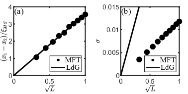
We note that the similarity in bulk free energy landscape likely leads to the similarity in solutions for LdG and the molecular field theory. Anisotropic effects have yet to be analyzed for our model, for which it is known for LdG there is nonzero biaxiality at interfaces Popa-Nita et al. 1997. This will be the subject of a future study.

IV.3 Tactoids
We consider a two-dimensional square domain of size . We set , , and at the outer boundary, where is the polar angle and is the winding number of . We set and . As initial conditions we set within a disc centered at the origin of radius .
By “tactoid” we refer to a two-phase domain separated by an interface. In the isotropic region . We consider distorted boundary conditions to ensure an interface forms in the simulation. Because the director can vary as a function of position in two dimensions, the boundary conditions imposed will change the size and shape of the object under consideration. Since we are only considering isotropic gradients in the elastic free energy, there is no anchoring term at the interface, i.e. there is not a difference in energy based on the orientation of the molecules relative to the interface. Thus, we expect the tactoids to be cylindrical. The topology of the boundary conditions does impact the size of the tactoids, however. This is due to a balance between two energies: the surface tension, which in two dimensions is proportional to , the radius of the tactoid, and the elastic energy in the nematic region from Oseen-Frank which is proportional to . Due to the symmetry of the molecules, half integer is allowed and costs four times less director distortion energy than integer . Hence, we expect that tactoids with integer boundary conditions should be approximately four times larger than those with half integer boundary conditions.
In Fig. 6, we show equilibrium configurations for boundary conditions with and . In both cases an isotropic region with is present at the center of the computational domain. As expected, both configurations are cylindrical in shape and we find that for the configuration and for the configuration. To find the radii we take a cut from the center of the tactoid to the outer boundary and find the point where . It should be noted that LdG, in the one-constant approximation in elastic energy, gives similar results in terms of the size and shape of tactoids.
It is known for the LdG bulk free energy with anisotropic elastic free energies that the shape of the tactoids also changes due to anchoring at the interface Golovaty et al. 2019. Anisotropic effects on the shape of tactoids in the molecular field theory will be the subject of a future study.
IV.4 Nematic Disclinations
We consider next the case of disclination lines in thin films. We consider a two-dimensional square of size . For all calculations and , so nematic ordering is energetically advantageous. At the outer boundary we fix the system to be uniaxial () and fix the director orientation, . The initial configuration is with everywhere.
In Fig. 7 we show the director profile, and the radial profile of equilibrium and from the center of a disclination to the boundary of the domain for the parameter . For the director, outside the core. Much like solutions for the LdG free energy, we see a disclination core that is biaxial Meiboom et al. 1983; Schopohl and Sluckin 1987. The biaxiality of the core was explained topologically by Lyuksyutov, assuming a LdG bulk free energy Lyuksyutov 1978. Using this free energy for analysis, one can define a “biaxial length” scale for the disclinations, , where is on the order of the Frank constants and is the parameter associated with the cubic term in the LdG bulk energy, Eq. (18). For distances from the core smaller than , the elastic energy becomes comparable to the cubic term in the LdG free energy and the system can remove the elastic singularity by becoming biaxial, since a biaxial order parameter can remove the singularity. We note that at the core, in both models. Using the parametrization from Eq. (8), one can show that this is interpreted as a uniaxial order parameter, but for a disc if or a rod aligned with the z-axis if . For both models, at the core. Thus, we interpret the biaxial solution as a macroscopic “transformation” of rods far away from the core to discs at the core. Microscopically, the probability distribution describing individual molecules becomes more and more spread out in the x-y plane in an attempt to alleviate the elastic energy singularity.

We emphasize that it is not obvious that the molecular field theory should give biaxial core solutions for the disclinations since, by construction, the model is markedly different from LdG. While LdG is an expansion of a macroscopic order parameter, the model here is based on a microscopic description. Because of this, it is difficult to quantitatively compare the solutions for the disclinations given by the two models. While we note that the spatial extent of the biaxiality for the disclinations is on the order of the radius of the defects, there is not a cubic term in the free energy to define a length such as . Instead, this behavior is induced by the single particle partition function which appears in Eq. (14) since the Maier-Saupe energy is purely quadratic in .
Another aspect of the disclinations that we can compare, at least qualitatively, to the LdG model is the scaling of the radius of disclinations with temperature. To find the radius, we take a cut from the center of the disclination to the boundary and find the point where . The results are plotted in Fig. 8. We show both the scaling for the molecular field theory and for results given by LdG. It can be seen that the scaling is similar for both models in a wide range of temperatures up to the coexistence temperature, where the isotropic phase becomes energetically favorable.
We are currently investigating the effects of anisotropic elastic free energies on disclinations. It is known that the director structure becomes less symmetric away from the disclination core if the Frank constants for bend and splay are not equal, and recent experiments have found anisotropic core structures Zhou et al. 2017.

V Conclusion
In this work, we have presented a computational implementation of the model of reference Ball and Majumdar 2010. We show that the model can be interpreted as replacing direct interactions between molecules via an effective interaction field in the mean field approximation. Further, we investigate the similarity between the free energy of this molecular field theory and the LdG free energy and compare solutions given by both for the cases of interfaces, tactoids, and topological defects. We find that all have qualitatively similar results which is an interesting result given that the construction of the two models is very different.
This model allows for a more fundamental understanding of the underlying microscopic and mesoscopic physics at play, and can serve as an alternative to the LdG free energy when describing systems with inhomogeneous ordering. The extension of the Maier-Saupe model to a field theory allows us to understand not just the phase transition but also inhomogeneous configurations, and can possibly be used to describe experiments like those of Refs. Zhou et al. 2017; Kim et al. 2013.
Moving forward, we are currently investigating the results of adding anisotropy to the elastic free energy, which has been done to some extent for the LdG model Golovaty et al. 2019. Importantly, however, one can consider in this framework the values of the elastic constants for chromonics that have been determined experimentally Zhou et al. 2014, while avoiding boundedness issues in LdG theory when bend and splay constants are different. Further, because of the microscopic nature of the model, one can, in principle, use a more physically realistic Hamiltonian to describe the molecular system, as opposed to the effective Maier-Saupe Hamiltonian that is used here. One can also generalize the computations to more complex molecules, such as plate-like molecules, by modifying Eq. (1).
Acknowledgements.
We are indebted to Shawn Walker and Sergij Shiyanovskii for useful discussions. This research is supported by the National Science Foundation under contract DMR-1838977, and by the Minnesota Supercomputing Institute.References
- de Gennes (1975) P. G. de Gennes, The Physics of Liquid Crystals (Oxford University Press, 1975).
- Selinger (2018) J. V. Selinger, Interpretation of saddle-splay and the Oseen-Frank free energy in liquid crystals, Liquid Crystals Reviews 6, 129 (2018).
- Lazo et al. (2014) I. Lazo, C. Peng, J. Xiang, S. V. Shiyanovskii, and O. D. Lavrentovich, Liquid crystal-enabled electroosmosis through spatial charge separation in distorted regions as a novel mechanism of electrokinetics, Nat. Commun. 5, 5033 (2014).
- Peng et al. (2015) C. Peng, Y. Guo, C. Conklin, J. Viñals, S. V. Shiyanovskii, Q.-H. Wei, and O. D. Lavrentovich, Liquid crystals with patterned molecular orientation as an electrolytic active medium, Phys. Rev. E 92, 052502 (2015).
- Peng et al. (2018) C. Peng, T. Turiv, Y. Guo, Q.-H. Wei, and O. D. Lavrentovich, Sorting and separation of microparticles by surface properties using liquid crystal-enabled electro-osmosis, Liq. Cryst. 45, 1936 (2018).
- Mostajeran (2015) C. Mostajeran, Curvature generation in nematic surfaces, Phys. Rev. E 91, 062405 (2015).
- Babakhanova et al. (2018) G. Babakhanova, T. Turiv, Y. Guo, M. Hendrikx, Q.-H. Wei, A. P. Schenning, D. J. Broer, and O. D. Lavrentovich, Liquid crystal elastomer coatings with programmed response of surface profile, Nat. Commun. 9, 456 (2018).
- Genkin et al. (2017) M. M. Genkin, A. Sokolov, O. D. Lavrentovich, and I. S. Aranson, Topological defects in a living nematic ensnare swimming bacteria, Phys. Rev. X 7, 011029 (2017).
- Hokmabad et al. (2019) B. V. Hokmabad, K. A. Baldwin, C. Krüger, C. Bahr, and C. C. Maass, Topological stabilization and dynamics of self-propelling nematic shells, Phys. Rev. Lett. 123, 178003 (2019).
- Yeh and Gu (2009) P. Yeh and C. Gu, Optics of Liquid Crystal Displays (Wiley, 2009).
- Collings et al. (2010) P. Collings, A. Dickinson, and E. Smith, Molecular aggregation and chromonic liquid crystals, Liquid Crystals 37, 701 (2010).
- Collings et al. (2015) P. J. Collings, J. N. Goldstein, E. J. Hamilton, B. R. Mercado, K. J. Nieser, and M. H. Regan, The nature of the assembly process in chromonic liquid crystals, Liquid Crystal Reviews 3, 1 (2015).
- Kim et al. (2013) Y. K. Kim, S. V. Shiyanovskii, and O. D. Lavrentovich, Morphogenesis of defects and tactoids during isotropic-nematic phase transition in self-assembled lyotropic chromonic liquid crystals, J. Phys.: Condens. Matter 25, 404202 (2013).
- Zhou et al. (2017) S. Zhou, S. V. Shiyanovskii, H.-S. Park, and O. D. Lavrentovich, Fine structure of the topological defect cores studied for disclinations in lyotropic chromonic liquid crystals, Nat. Commun. 8, 14974 (2017).
- Frank (1958) F. Frank, On the theory of liquid crystals, Discuss. Faraday Soc. 25, 19 (1958).
- Zhou et al. (2014) S. Zhou, K. Neupane, Y. A. Nastishin, A. R. Baldwin, S. V. Shiyanovskii, O. D. Lavrentovich, and S. Sprunt, Elasticity, viscocity, and orientational fluctuations of a lyotropic chromonic nematic liquid crystal disodium cromoglycate, Soft Matter 10, 6571 (2014).
- Leslie (1966) F. M. Leslie, Some constitutive equations for anisotropic fluids, J. Mech. Appl. Math. 19, 357 (1966).
- Ericksen (1991) J. L. Ericksen, Liquid crystals with variable degree of orientation, Arch. for Rational Mech. Anal. 113, 97 (1991).
- Zhang et al. (2018) C. Zhang, A. Acharya, N. J. Walkington, and O. D. Lavrentovich, Computational modelling of tactoid dynamics in chromonic liquid crystals, Liq. Cryst. 45, 1084 (2018).
- Meiboom et al. (1983) S. Meiboom, M. Sammon, and W. F. Brinkman, Lattice of disclinations: The structure of the blue phases of choloesteric liquid crystals, Phys. Rev. A 27, 438 (1983).
- Golovaty et al. (2019) D. Golovaty, Y.-K. Kim, O. D. Lavrentovich, M. Novack, and P. Sternberg, Phase transitions in nematics: textures with tacoids and disclinations, e-print arXiv:1902.06342v1[cond-mat.soft] (2019).
- Popa-Nita et al. (1997) V. Popa-Nita, T. Sluckin, and A. Wheeler, Statics and kinematics at the nematic-isotropic interface: effects of biaxiality, Journal de Physique II 7, 1225 (1997).
- Gramsbergen et al. (1986) E. F. Gramsbergen, L. Longa, and W. H. de Jeu, Landau theory of the nematic-isotropic phase transition, Physics Reports 135, 195 (1986).
- Lubensky (1970) T. C. Lubensky, Molecular description of nematic liquid crystals, Phys. Rev. A 2, 2497 (1970).
- Longa et al. (1987) L. Longa, D. Monselesan, and H. R. Trebin, An extension of the Landau-Ginzberg-de Gennes theory for liquid crystals, Liq. Cryst. 2, 769 (1987).
- Ball and Majumdar (2010) J. M. Ball and A. Majumdar, Nematic liquid crystals: from Maier-Saupe to a continuum theory, Mol. liq. Cryst. 525, 1 (2010).
- Maier and Saupe (1959) W. Maier and A. Saupe, A simple molecular statistical theory of the nematic liquid-crystalline phase, I. Z. Naturf. 14, 882 (1959).
- Chiccoli et al. (2019) C. Chiccoli, L. R. Evangelista, P. Pasini, G. Skačej, R. T. de Souza, and C. Zannoni, Influence of boundary conditions on the order and defects of biaxial nematic droplets, Phys. Rev. E 100, 032702 (2019).
- Selinger (2016) J. V. Selinger, Liquid crystals, in Introduction to the Theory of Soft Matter: From Ideal Gases to Liquid Crystals (Springer International Publishing, 2016) pp. 131–182.
- Katriel et al. (1986) J. Katriel, G. F. Kventsel, G. R. Luckhurst, and T. Sluckin, Free energies in the Landau and molecular field approaches, Liq. Cryst. 1, 337 (1986).
- Bauman and Phillips (1986) P. Bauman and D. Phillips, Regularity and the behavior of eigenvalues for minimizers of a constrained Q-tensor energy for liquid crystals, Calc. Var. 55, 81 (1986).
- Pismen (1999) L. M. Pismen, Vortices in Nonlinear Fields (Oxford University Press, 1999).
- Mottram and Newton (2014) N. J. Mottram and C. J. Newton, Introduction to Q-tensor theory, e-print arXiv:1409.3542v2 [cond-mat.soft] (2014).
- Sen and Sullivan (1987) A. K. Sen and D. E. Sullivan, Landau-de Gennes theory of wetting and orientational transitions at a nematic-liquid–substrate interface, Phys. Rev. A 35, 1391 (1987).
- Press et al. (2002) W. H. Press, S. A. Teukolsky, W. T. Vetterling, and B. P. Flannery, Numerical Recipes in C++ The Art of Scientific Computing, 2nd ed. (Cambridge University Press, 2002).
- Schimming (2020) C. D. Schimming, MATLAB code for the numerical solution of the Maier-Saupe field theory, http://hdl.handle.net/11299/211301 (2020).
- Schopohl and Sluckin (1987) N. Schopohl and T. Sluckin, Defect core structure in nematic liquid crystals, Phys. Rev. Lett. 59, 22 (1987).
- Lyuksyutov (1978) I. F. Lyuksyutov, Topological instability of singularities at small distances in nematics, Zh. Eksp. Teor. Fiz. 75, 358 (1978).