Edge-Matching Graph Contractions and their Interlacing PropertiesJournal: Linear Algebra and its Applications

Noam Leiter Email: noaml@campus.technion.ac.il Address: Faculty of Aerospace Engineering, Technion, Haifa 32000 Israel Daniel Zelazo Email: dzelazo@technion.ac.il Address: Faculty of Aerospace Engineering, Technion, Haifa 32000 Israel

Abstract

For a given graph $\mathcal{G}$ of order $n$ with $m$ edges, and a real symmetric matrix associated to the graph, $M\left(\mathcal{G}\right)\in\mathbb{R}^{n\times n}$ , the interlacing graph reduction problem is to find a graph $\mathcal{G}_{r}$ of order $r<n$ such that the eigenvalues of $M\left(\mathcal{G}_{r}\right)$ interlace the eigenvalues of $M\left(\mathcal{G}\right)$ . Graph contractions over partitions of the vertices are widely used as a combinatorial graph reduction tool. In this study, we derive a graph reduction interlacing theorem based on subspace mappings and the minmax theory. We then define a class of edge-matching graph contractions and show how two types of edge-matching contractions provide Laplacian and normalized Laplacian interlacing. An $\mathcal{O}\left(mn\right)$ algorithm is provided for finding a normalized Laplacian interlacing contraction and an $\mathcal{O}\left(n^{2}+nm\right)$ algorithm is provided for finding a Laplacian interlacing contraction.

Keywords:

Spectral clustering, Laplacian interlacing, Graph contractions

1 Introduction

The effect of combinatorial operations on graph spectra is an evolving branch of graph theory, linking together combinatorial graph theory with the spectral analysis of the algebraic structures of graphs. In general, there is an interest to understand how certain graph reduction operations relate to spectral and combinatorial properties. Of particular interest are reductions that satisfy an interlacing property between algebraic graph representations. Interlacing properties of algebraic structures of graphs have been shown to have combinatorial interpretations. Haemers used the adjacency and Laplacian matrix interlacing to provide combinatorical results on the chromatic number and spectral bounds [1]. The neighborhood reassignment operation has been shown to provide an interlacing of the normalized Laplacian [2], and Chen et al. provide an interlacing result on contracted normalized Laplacians [3].

Partitioning the vertices of a graph is a combinatorial operation extensively studied in graph theory in the context of graph clustering [4] and network communities [5], and for spectral clustering methods [6]. Partitioning combined with node and edge contractions along those partitions lead to reduced order graphs. In this direction, we define edge-matching contractions as a class of graph contractions with a one-to-one correspondence of a subset of edges in the full order graph to those in the contracted graph. We then explore two types of edge-matching contractions, cycle invariant contractions and node-removal equivalent contractions. Cycle-invariant contractions preserve the cycle structure of the graph in the contracted graph, and node-removal equivalent contractions are cases where a contraction can be obtained also from a node-removal operation. We show how contraction of these types lead to interlacing of the normalized-Laplacian and Laplacian graph matrices. Two algorithms of complexity $\mathcal{O}\left(mn\right)$ and $\mathcal{O}\left(n^{2}+nm\right)$ are then provided for finding, if they exist, a cycle-invariant contraction and a node-removal equivalent contraction respectively for a given graph with $n$ vertices and $m$ edges.

The remaining sections of this paper are as follows. In Section 2, the interlacing graph reduction problem is presented and an interlacing graph reduction theorem is derived. In Section 3 we formulate the graph contraction operation for simple undirected graphs, and introduce the class of edge-matching graph contractions and two sub-classes of cycle-invariant and node-removal equivalent graph contractions. In Section 4, the interlacing graph reduction problem is solved for these two classes for the Laplacian and normalized-Laplacian matrices, and Section 5 provides case studies of the interlacing methods.

Preliminaries

The integer set $\left\{1,\ldots,n\right\}$ is denoted as $\left[1,n\right]$ . An undirected graph $\mathcal{G}=\left(\mathcal{V},\mathcal{E}\right)$ consists of a vertex set $\mathcal{V}\left(\mathcal{G}\right)$ , and an edge set $\mathcal{E}\left(\mathcal{G}\right)=\{\epsilon_{1},\ldots,\epsilon_{|\mathcal{E}|}\}$ with $\epsilon_{k}\in\mathcal{V}{}^{2}$ . The order of the graph is the number of vertices $|\mathcal{V}\left(\mathcal{G}\right)|$ . Two nodes $u,v\in\mathcal{V}\left(\mathcal{G}\right)$ are adjacent if they are the endpoints of an edge, and we denote this by $u\sim v$ . The neighborhood $\mathcal{N}_{v}\left(\mathcal{G}\right)$ is the set of all nodes adjacent to $v$ in $\mathcal{G}$ . The degree of a node $v$ , denoted $d_{v}\left(\mathcal{G}\right)$ , is the number of nodes adjacent to it, $d_{v}\left(\mathcal{G}\right)=\left|\mathcal{N}_{v}\left(\mathcal{G}\right)\right|$ . A path in a graph is a sequence of distinct adjacent nodes. A simple cycle is a path with an additional edge such that the first and last vertices are repeated. A graph $\mathcal{G}$ is connected if we can find a path between any pair of nodes. A simple graph does not include self-loops or duplicate edges. A multi-graph is a graph that may include duplicate edges. We denote $\mathcal{G}\backslash\mathcal{V}_{R}$ as the graph obtained from $\mathcal{G}$ by removing all nodes $v\in\mathcal{V}_{R}\subset\mathcal{V}$ from $\mathcal{V}\left(G\right)$ and removing all edges in $\mathcal{E}\left(\mathcal{G}\right)$ adjacent to $v$ . We denote $\mathcal{G}\backslash\mathcal{E}_{R}$ as a graph obtained from $\mathcal{G}$ by removing all edges $\epsilon\in\mathcal{E}_{R}$ from $\mathcal{E}\left(G\right)$ . A subgraph $\mathcal{G}_{S}=\left(\mathcal{V}_{S},\mathcal{E}_{S}\right)$ of a graph $\mathcal{G}=\left(\mathcal{V},\mathcal{E}\right)$ , denoted as $\mathcal{G}_{S}\subseteq\mathcal{G}$ , is any graph such that $\mathcal{V}_{S}\subseteq\mathcal{V}$ and $\mathcal{E}_{S}\subseteq\mathcal{E}\cap\mathcal{V}_{S}^{2}$ . An induced subgraph $\mathcal{G}\left[\mathcal{V}_{S}\right]$ is a subgraph $\mathcal{G}_{S}\subseteq\mathcal{G}$ such that $\mathcal{E}_{S}=\mathcal{E}_{\mathcal{G}}\cap\mathcal{V}_{S}^{2}$ . An induced subgraph $\mathcal{G}\left[\mathcal{V}_{S}\right]$ is a connected component of $\mathcal{G}$ if it is connected and no node in $\mathcal{V}_{S}$ is adjacent to a node in $\mathcal{V}\left(\mathcal{G}\right)\backslash\mathcal{V}_{S}$ . The set $\mathbb{T}\left(\mathcal{G}\right)$ denotes the set of all spanning trees of a connected graph $\mathcal{G}$ . For $\mathcal{T}\in\mathbb{T}\left(\mathcal{G}\right)$ , the co-tree graph $\mathcal{G}\backslash\mathcal{E}\left(\mathcal{T}\right)$ is denoted as $\mathcal{C}\left(\mathcal{T}\right)$ [7].

2 Interlacing Graph Reductions

Graph matrices are algebraic representations of graphs, and the spectral and algebraic properties of these matrices can provide insights about combinatorial properties of the underlying graph, e.g., Fiedler’s seminal results on the Laplacian algebraic connectivity [8]. The interlacing property of matrices has been extensively studied with classic algebraic results such as the Poincare separation theorem [9, p. 119], and matrix combinatorial results such as the relation of equitable partitions with tight interlacing [10]. Here we study what types of reduced graphs have interlacing graph matrices.

The spectrum of a real symmetric matrix $A\in\mathbb{R}^{n\times n}$ is the set of eigenvalues $\left\{\lambda_{k}\left(A\right)\right\}_{k=1}^{n}$ where $\lambda_{k}\left(A\right)$ is the $k$ th eigenvalue of $A$ in ascending order. Let $A\in\mathbb{R}^{n\times n}$ and $B\in\mathbb{R}^{r\times r}$ be real symmetric matrices with $0<r<n$ . Then the eigenvalues of $B$ interlace the eigenvalues of $A$ , denoted $B\propto A$ , if $\lambda_{k}\left(A\right)\leq\lambda_{k}\left(B\right)\leq\lambda_{n-r+k}\left(A\right)$ for $k=1,2,\ldots,r$ . The interlacing is tight if $\lambda_{k}\left(A\right)=\lambda_{k}\left(B\right)$ or $\lambda_{k}\left(B\right)=\lambda_{n-r+k}\left(A\right)$ for $k=1,2,\ldots,r$ . It is straight forward to show that interlacing is a transitive property.

Proposition 1.

Let $A_{1}\in\mathbb{R}^{n_{1}\times n_{1}}$ , $A_{2}\in\mathbb{R}^{n_{2}\times n_{2}}$ and $A_{3}\in\mathbb{R}^{n_{3}\times n_{3}}$ be real symmetric matrices with $0<n_{3}<n_{2}<n_{1}$ . If $A_{3}\propto A_{2}$ and $A_{2}\propto A_{1}$ , then $A_{3}\propto A_{1}$ .

Proof.

From $A_{3}\propto A_{2}$ and $A_{2}\propto A_{1}$ we have $\lambda_{k}\left(A_{2}\right)\leq\lambda_{k}\left(A_{3}\right)\leq\lambda_{n_{2}-n_{3}+k}\left(A_{2}\right)$ for $k=1,2,\ldots,n_{3}$ and $\lambda_{l}\left(A_{1}\right)\leq\lambda_{l}\left(A_{2}\right)\leq\lambda_{n_{1}-n_{2}+l}\left(A_{1}\right)$ for $l=1,2,\ldots,n_{2}$ . From $l=k$ we get $\lambda_{k}\left(A_{1}\right)\leq\lambda_{k}\left(A_{2}\right)\leq\lambda_{k}\left(A_{3}\right)$ , and from $l=n_{2}-n_{3}+k$ we get $\lambda_{k}\left(A_{3}\right)\leq\lambda_{n_{2}-n_{3}+k}\left(A_{2}\right)\leq\lambda_{n_{1}-n_{3}+k}\left(A_{1}\right)$ , such that $\lambda_{k}\left(A_{1}\right)\leq\lambda_{k}\left(A_{3}\right)\leq\lambda_{n_{1}-n_{3}+k}\left(A_{1}\right)$ for $k=1,2,\ldots,n_{3}$ and we obtain that $A_{3}\propto A_{1}$ .∎

The most commonly studied matrices in algebraic graph theory are the adjacency matrix $A\left(\mathcal{G}\right)\in\mathbb{R}^{\left|\mathcal{V}\right|\times\left|\mathcal{V}\right|}$ , the Laplacian matrix $L\left(\mathcal{G}\right)\in\mathbb{R}^{\left|\mathcal{V}\right|\times\left|\mathcal{V}\right|}$ and the normalized Laplacian matrix $\mathcal{L}\left(\mathcal{G}\right)\in\mathbb{R}^{\left|\mathcal{V}\right|\times\left|\mathcal{V}\right|}$ , all of which are real symmetric matrices. They are defined below, where each row and column is indexed by a vertex in the graph $\mathcal{G}$ [7],

[A(\mathcal{G})]_{uv}=\left\{\begin{array}[]{cl}1,&u\sim v\\ 0,&\mbox{otherwise}\end{array}\right.,

[L(\mathcal{G})]_{uv}=\left\{\begin{array}[]{cl}d_{u}\left(\mathcal{G}\right),&u=v\\ -1&u\sim v\\ 0,&\mbox{otherwise}\end{array}\right.,

and

[\mathcal{L}(\mathcal{G})]_{uv}=\left\{\begin{array}[]{cl}1,&u=v\\ -\left(\sqrt{d_{u}\left(\mathcal{G}\right)d_{v}\left(\mathcal{G}\right)}\right)^{-1}&u\sim v\\ 0,&\mbox{otherwise}\end{array}\right..

We now extend the notion of spectral interlacing properties to graphs.

Definition 1 (interlacing graphs).

Consider two graphs $\mathcal{G}_{n}$ and $\mathcal{G}_{r}$ of order $n$ and $r$ respectively, with $n>r$ , and let $M(\mathcal{G})\in\mathbb{R}^{n\times n}$ be any real symmetric matrix associated with the graph $\mathcal{G}$ . We say that the two graphs are $M$ -interlacing if $M\left(\mathcal{G}_{r}\right)\propto M\left(\mathcal{G}_{n}\right)$ , and denote the property by $\mathcal{G}_{r}\propto_{M}\mathcal{G}_{n}$ .

A problem arising naturally from the definition of interlacing graphs is the interlacing graph reduction problem.

Problem 1 (interlacing graph reduction).

Consider a graph $\mathcal{G}_{n}$ of order $n$ and let $M(\mathcal{G})\in\mathbb{R}^{n\times n}$ be any real symmetric matrix associated with the graph $\mathcal{G}$ . Find a graph $\mathcal{G}_{r}$ of a given order $r<n$ such that $\mathcal{G}_{r}\propto_{M}\mathcal{G}_{n}$ .

Finding a solution to Problem 1 may be numerically intractable for a moderate number of nodes, as the number $c_{r}$ of simple connected graphs of order $r$ increases exponentially according to the recurrence $\sum_{k}\binom{r}{k}kc_{k}2^{\binom{r-k}{2}}=r2^{\binom{r}{2}}$ for $r\geq 1$ [11, p.87], e.g., for $r=1,\ldots,6$ , $c_{r}=1,\,1,\,4,\,38,\,728,\,26704$ .

A powerful tool for proving interlacing results is the Courant-Fischer theorem, e.g., that a symmetric matrix and a principle submatrix of that matrix interlace [1], which leads to an adjacency interlacing theorem for node-removal graph reductions:

Theorem 1 (Adjacency interlacing node-removal).

Consider a graph $\mathcal{G}$ and a node subset $\mathcal{V}_{S}\subset\mathcal{V}\left(\mathcal{G}\right)$ . Then $\mathcal{G}\backslash\mathcal{V}_{S}\propto_{A}\mathcal{G}$ .

Proof.

The matrix $A\left(\mathcal{G}\backslash\mathcal{V}_{S}\right)$ is a principle submatrix of $A\left(\mathcal{G}\right)$ , therefore, $\mathcal{G}\backslash\mathcal{V}_{S}\propto_{A}\mathcal{G}$ .∎

Utilizing the Courant-Fischer theorem and the following $\min\max$ inequalities (Proposition 2) an interlacing graph reduction theorem is derived. We first introduce some notations to simplify the statement. A $k$ -dimensional subspace of $\mathbb{R}^{n}$ is denoted as $\mathcal{F}_{n}^{\left(k\right)}$ . For an $r$ -dimensional subspace $\mathcal{F}_{n}^{(r)}$ , we define the injective map $p_{\mathcal{F}_{n}^{\left(r\right)}}:\mathbb{R}^{r}\rightarrow\mathbb{R}^{n}$ , such that $x\in\mathbb{R}^{r}\mapsto y\in\mathcal{F}_{n}^{(r)}$ .

Theorem 2 (Courant-Fischer [12]).

Consider a real symmetric matrix $M\in\mathbb{R}^{n\times n}$ , then for $k\in\left[1,n\right]$

\lambda_{k}\left(M\right)=\underset{\mathcal{F}_{n}^{\left(n-k+1\right)}}{\max}\;\underset{\begin{subarray}{c}x\in\mathcal{F}_{n}^{\left(n-k+1\right)}\\ x\neq 0\end{subarray}}{\min}R\left(M,x\right),

and

\lambda_{k}\left(M\right)=\underset{\mathcal{F}_{n}^{\left(k\right)}}{\min}\;\underset{\begin{subarray}{c}x\in\mathcal{F}_{n}^{\left(k\right)}\\ x\neq 0\end{subarray}}{\max}R\left(M,x\right),

where $R\left(M,x\right)\triangleq\frac{x^{T}Mx}{x^{T}x}$ is the Rayleigh quotient.

Proposition 2.

Consider a subspace $\mathcal{F}_{n}^{(r)}$ for $r<n$ , and let $f\left(x\right):\mathbb{R}^{n}\rightarrow\mathbb{R}$ be a real-valued function that attains a minimum and a maximum on $\mathbb{R}^{n}\backslash\left\{0\right\}$ . Then the following holds for $k\in\left[1,r\right]$ :

i)

$\underset{\mathcal{F}_{n}^{\left(n-k+1\right)}}{\max}\;\underset{\begin{subarray}{c}x\in\mathcal{F}_{n}^{\left(n-k+1\right)}\\ x\neq 0\end{subarray}}{\min}f\left(x\right)\leq\max\limits_{\mathcal{F}_{r}^{\left(r-k+1\right)}}\;\min\limits_{\begin{subarray}{c}\tilde{x}\in\mathcal{F}_{r}^{\left(r-k+1\right)}\\ \tilde{x}\neq 0\end{subarray}}f\left(p_{\mathcal{F}_{n}^{\left(r\right)}}\left(\tilde{x}\right)\right)$ ,
ii)

$\min\limits_{\mathcal{F}_{n}^{\left(n-r+k\right)}}\;\max\limits_{\begin{subarray}{c}x\in\mathcal{F}_{n}^{\left(n-r+k\right)}\\ x\neq 0\end{subarray}}f\left(x\right)\geq\min\limits_{\mathcal{F}_{r}^{\left(k\right)}}\;\max\limits_{\begin{subarray}{c}\tilde{x}\in\mathcal{F}_{r}^{\left(k\right)}\\ \tilde{x}\neq 0\end{subarray}}f\left(p_{\mathcal{F}_{n}^{\left(r\right)}}\left(\tilde{x}\right)\right)$ .

Proof.

We first prove ( $i$ ). Let $s\equiv n-k+1$ . For all $\mathcal{F}_{n}^{\left(s\right)}\subseteq\mathbb{R}^{n}$ ,

	$\displaystyle\underset{\begin{subarray}{c}x\in\mathcal{F}_{n}^{\left(s\right)}\\ x\neq 0\end{subarray}}{\min}f\left(x\right)$	$\displaystyle=\min\left\{\min\limits_{\begin{subarray}{c}x\in\mathcal{F}_{n}^{\left(s\right)}\cap\mathcal{F}_{n}^{\left(r\right)}\\ x\neq 0\end{subarray}}f\left(x\right),\;\min\limits_{\begin{subarray}{c}x\in\mathcal{F}_{n}^{\left(s\right)}\backslash\left\{\mathcal{F}_{n}^{\left(s\right)}\cap\mathcal{F}_{n}^{\left(r\right)}\right\}\\ x\neq 0\end{subarray}}f\left(x\right)\right\}$
		$\displaystyle\leq\min\limits_{\begin{subarray}{c}x\in\mathcal{F}_{n}^{\left(s\right)}\cap\mathcal{F}_{n}^{\left(r\right)}\\ x\neq 0\end{subarray}}f\left(x\right),$

and we obtain that

\underset{\mathcal{F}_{n}^{\left(s\right)}}{\max}\;\underset{\begin{subarray}{c}x\in\mathcal{F}_{n}^{\left(s\right)}\\ x\neq 0\end{subarray}}{\min}f\left(x\right)\leq\max\limits_{\mathcal{F}_{n}^{\left(s\right)}}\;\min\limits_{\begin{subarray}{c}x\in\mathcal{F}_{n}^{\left(s\right)}\cap\mathcal{F}_{n}^{\left(r\right)}\\ x\neq 0\end{subarray}}f\left(x\right).

(1)

Since $k\leq r$ , then $s=n-k+1>n-r$ and

\dim\left(\mathcal{F}_{n}^{\left(s\right)}\cap\mathcal{F}_{n}^{\left(r\right)}\right)\geq s-\left(n-r\right).

Therefore,

\displaystyle\max\limits_{\mathcal{F}_{n}^{\left(s\right)}}\;\min\limits_{\begin{subarray}{c}x\in\mathcal{F}_{n}^{\left(s\right)}\cap\mathcal{F}_{n}^{\left(r\right)}\\ x\neq 0\end{subarray}}f\left(x\right)=\max\limits_{\mathcal{F}_{n}^{\left(s-\left(n-r\right)\right)}\subseteq\mathcal{F}_{n}^{\left(r\right)}}\;\min\limits_{\begin{subarray}{c}x\in\mathcal{F}_{n}^{\left(s-\left(n-r\right)\right)}\\ x\neq 0\end{subarray}}f\left(x\right).

For each $\mathcal{F}_{n}^{\left(s-\left(n-r\right)\right)}\subseteq\mathcal{F}_{n}^{\left(r\right)}$ we can find $\mathcal{\tilde{F}}_{r}^{\left(s-\left(n-r\right)\right)}\subseteq\mathbb{R}^{r}$ that is mapped to it by $p_{\mathcal{F}_{n}^{\left(r\right)}}\left(\tilde{x}\right)$ ,

\mathcal{\tilde{F}}_{r}^{\left(s-\left(n-r\right)\right)}=\left\{\tilde{x}\in\mathbb{R}^{r}|p_{\mathcal{F}_{n}^{\left(r\right)}}\left(\tilde{x}\right)\in\mathcal{F}_{n}^{\left(s-\left(n-r\right)\right)}\right\},

such that

\displaystyle\min\limits_{\begin{subarray}{c}x\in\mathcal{F}_{n}^{\left(s-\left(n-r\right)\right)}\\ x\neq 0\end{subarray}}f\left(x\right)=\min\limits_{\begin{subarray}{c}\tilde{x}\in\tilde{\mathcal{F}}_{r}^{\left(s-\left(n-r\right)\right)}\\ \tilde{x}\neq 0\end{subarray}}f\left(p_{\mathcal{F}_{n}^{\left(r\right)}}\left(\tilde{x}\right)\right).

Maximizing over all $\mathcal{F}_{n}^{\left(s-\left(n-r\right)\right)}\subseteq\mathcal{F}_{n}^{\left(r\right)}$ we obtain

\displaystyle\max\limits_{\mathcal{F}_{n}^{\left(s-\left(n-r\right)\right)}\subseteq\mathcal{F}_{n}^{\left(r\right)}}\;\min\limits_{\begin{subarray}{c}x\in\mathcal{F}_{n}^{\left(s-\left(n-r\right)\right)}\\ x\neq 0\end{subarray}}f\left(x\right)

\displaystyle=\max\limits_{\mathcal{F}_{r}^{\left(s-\left(n-r\right)\right)}}\;\min\limits_{\begin{subarray}{c}\tilde{x}\in\tilde{\mathcal{F}}_{r}^{\left(s-\left(n-r\right)\right)}\\ \tilde{x}\neq 0\end{subarray}}f\left(p_{\mathcal{F}_{n}^{\left(r\right)}}\left(\tilde{x}\right)\right),

and

\max\limits_{\mathcal{F}_{n}^{\left(n-k+1\right)}}\;\min\limits_{\begin{subarray}{c}x\in\mathcal{F}_{n}^{\left(n-k+1\right)}\cap\mathcal{F}_{n}^{\left(r\right)}\\ x\neq 0\end{subarray}}f\left(x\right)=\max\limits_{\mathcal{F}_{r}^{\left(r-k+1\right)}}\;\min\limits_{\begin{subarray}{c}\tilde{x}\in\tilde{\mathcal{F}}_{r}^{\left(r-k+1\right)}\\ \tilde{x}\neq 0\end{subarray}}f\left(p_{\mathcal{F}_{n}^{\left(r\right)}}\left(\tilde{x}\right)\right).

(2)

Equation (2) together with (1) completes the proof of ( $i$ ).

The proof of (ii) is as follows. Let $s\equiv n-r+k$ . For all $\mathcal{F}_{n}^{\left(s\right)}\subseteq\mathbb{R}^{n}$ ,

	$\displaystyle\max\limits_{\begin{subarray}{c}x\in\mathcal{F}_{n}^{\left(s\right)}\\ x\neq 0\end{subarray}}f\left(x\right)$	$\displaystyle=\max\left\{\max\limits_{\begin{subarray}{c}x\in\mathcal{F}_{n}^{\left(s\right)}\cap\mathcal{F}_{n}^{\left(r\right)}\\ x\neq 0\end{subarray}}f\left(x\right),\;\max\limits_{\begin{subarray}{c}x\in\mathcal{F}_{n}^{\left(s\right)}\backslash\left\{\mathcal{F}_{n}^{\left(s\right)}\cap\mathcal{F}_{n}^{\left(r\right)}\right\}\\ x\neq 0\end{subarray}}f\left(x\right)\right\}$
		$\displaystyle\geq\max\limits_{\begin{subarray}{c}x\in\mathcal{F}_{n}^{\left(s\right)}\cap\mathcal{F}_{n}^{\left(r\right)}\\ x\neq 0\end{subarray}}f\left(x\right),$

and

\min\limits_{\mathcal{F}_{n}^{\left(s\right)}}\;\max\limits_{\begin{subarray}{c}x\in\mathcal{F}_{n}^{\left(s\right)}\\ x\neq 0\end{subarray}}f\left(x\right)\geq\min\limits_{\mathcal{F}_{n}^{\left(s\right)}}\;\max\limits_{\begin{subarray}{c}x\in\mathcal{F}_{n}^{\left(s\right)}\cap\mathcal{F}_{n}^{\left(r\right)}\\ x\neq 0\end{subarray}}f\left(x\right).

(3)

Since $k\geq 1$ then $s=n-r+k>n-r$ and

\dim\left(\mathcal{F}_{n}^{\left(s\right)}\cap\mathcal{F}_{n}^{\left(r\right)}\right)\geq s-\left(n-r\right),

and we can then replace $\max\min$ with $\min\max$ in the above proof of (i) and obtain

\min\limits_{\mathcal{F}_{n}^{\left(n-r+k\right)}}\;\max\limits_{\begin{subarray}{c}x\in\mathcal{F}_{n}^{\left(n-r+k\right)}\cap\mathcal{F}_{n}^{\left(r\right)}\\ x\neq 0\end{subarray}}f\left(x\right)=\min\limits_{\mathcal{F}_{r}^{\left(k\right)}}\;\max\limits_{\begin{subarray}{c}\tilde{x}\in\mathcal{F}_{r}^{\left(k\right)}\\ \tilde{x}\neq 0\end{subarray}}f\left(p_{\mathcal{F}_{n}^{\left(r\right)}}\left(\tilde{x}\right)\right).

(4)

Equation (4) together with (3) completes the proof of ( $ii$ ). ∎

Theorem 3 (Interlacing graph reduction theorem).

Consider two graphs $\mathcal{G}_{n}$ and $\mathcal{G}_{r}$ of order $n$ and $r$ respectively, with $n>r$ , and let $M(\mathcal{G})\in\mathbb{R}^{n\times n}$ be any real symmetric matrix associated with the graph $\mathcal{G}$ . If there exists $r$ -dimensional subspaces $\mathcal{A},\mathcal{B}\subseteq\mathbb{R}^{n}$ such that $\forall x\in\mathbb{R}^{r}\backslash\left\{0\right\}$ ,

R\left(M\left(\mathcal{G}_{n}\right),p_{\mathcal{A}}\left(x\right)\right)\leq R\left(M\left(\mathcal{G}_{r}\right),x\right),

and

R\left(M\left(\mathcal{G}_{n}\right),p_{\mathcal{B}}\left(x\right)\right)\geq R\left(M\left(\mathcal{G}_{r}\right),x\right),

then $\mathcal{G}_{r}\propto_{M}\mathcal{G}_{n}$ .

Proof.

In order for $\mathcal{G}_{n}$ and $\mathcal{G}_{r}$ to be $M$ -interlacing (Definition 2) we must prove that $\lambda_{k}\left(M\left(\mathcal{G}_{n}\right)\right)\leq\lambda_{k}\left(M\left(\mathcal{G}_{r}\right)\right)\leq\lambda_{n-r+k}\left(M\left(\mathcal{G}_{n}\right)\right)$ for $k\in\left[1,r\right]$ . From the Courant–Fischer theorem (Theorem 2) we have

\lambda_{k}\left(M\left(\mathcal{G}_{n}\right)\right)=\underset{\mathcal{F}_{n}^{\left(n-k+1\right)}}{\max}\;\underset{\begin{subarray}{c}x\in\mathcal{F}_{n}^{\left(n-k+1\right)}\\ x\neq 0\end{subarray}}{\min}R\left(M\left(\mathcal{G}_{n}\right),x\right),

and from the min-max properties (Proposition 2) with $\mathcal{F}_{n}^{\left(r\right)}\equiv\mathcal{A}$ we have for $k\in\left[1,r\right]$ ,

\lambda_{k}\left(M\left(\mathcal{G}_{n}\right)\right)\leq\underset{\mathcal{F}_{r}^{\left(r-k+1\right)}}{\max}\;\underset{\begin{subarray}{c}x\in\mathcal{F}_{r}^{\left(r-k+1\right)}\\ x\neq 0\end{subarray}}{\min}R\left(M\left(\mathcal{G}_{n}\right),p_{\mathcal{A}}\left(x\right)\right).

Since $R\left(M\left(\mathcal{G}_{n}\right),p_{\mathcal{A}}\left(x\right)\right)\leq R\left(M\left(\mathcal{G}_{r}\right),x\right)$ , therefore,

	$\displaystyle\lambda_{k}\left(M\left(\mathcal{G}_{n}\right)\right)$	$\displaystyle\leq\underset{\mathcal{F}_{r}^{\left(r-k+1\right)}}{\max}\;\underset{\begin{subarray}{c}x\in\mathcal{F}_{r}^{\left(r-k+1\right)}\\ x\neq 0\end{subarray}}{\min}R\left(M\left(\mathcal{G}_{r}\right),x\right)$
		$\displaystyle=\lambda_{k}\left(M\left(\mathcal{G}_{r}\right)\right),$

and $\lambda_{k}\left(M\left(\mathcal{G}_{n}\right)\right)\leq\lambda_{k}\left(M\left(\mathcal{G}_{r}\right)\right)$ for $k\in\left[1,r\right]$ . In order to complete the interlacing proof it is left to show that $\lambda_{k}\left(M\left(\mathcal{G}_{r}\right)\right)\leq\lambda_{n-r+k}\left(M\left(\mathcal{G}_{n}\right)\right)$ for $k\in\left[1,r\right]$ . From the Courant–Fischer theorem (Theorem 2) we get

\lambda_{n-r+k}\left(M\left(\mathcal{G}_{n}\right)\right)=\underset{\mathcal{F}_{n}^{\left(n-r+k\right)}}{\min}\;\underset{\begin{subarray}{c}x\in\mathcal{F}_{n}^{\left(n-r+k\right)}\\ x\neq 0\end{subarray}}{\max}R\left(M\left(\mathcal{G}_{n}\right),x\right),

and from the min-max properties (Proposition 2) with $\mathcal{F}_{n}^{\left(r\right)}\equiv\mathcal{B}$ we have

\lambda_{n-r+k}\left(M\left(\mathcal{G}_{n}\right)\right)\geq\underset{\mathcal{F}_{r}^{\left(k\right)}}{\min}\;\underset{\begin{subarray}{c}x\in\mathcal{F}_{r}^{\left(k\right)}\\ x\neq 0\end{subarray}}{\max}R\left(M\left(\mathcal{G}_{n}\right),p_{\mathcal{B}}\left(x\right)\right).

Since $R\left(M\left(\mathcal{G}_{n}\right),p_{\mathcal{B}}\left(x\right)\right)\geq R\left(M\left(\mathcal{G}_{r}\right),x\right)$ , therefore,

	$\displaystyle\lambda_{n-r+k}\left(M\left(\mathcal{G}_{n}\right)\right)$	$\displaystyle\geq\underset{\mathcal{F}_{r}^{\left(k\right)}}{\min}\;\underset{\begin{subarray}{c}x\in\mathcal{F}_{r}^{\left(k\right)}\\ x\neq 0\end{subarray}}{\max}R\left(M\left(\mathcal{G}_{r}\right),x\right)$
		$\displaystyle=\lambda_{k}\left(M\left(\mathcal{G}_{r}\right)\right),$

and $\lambda_{k}\left(M\left(\mathcal{G}_{n}\right)\right)\leq\lambda_{n-r+k}\left(M\left(\mathcal{G}_{r}\right)\right)$ for $k\in\left[1,r\right]$ , completing the proof.∎

In the next section we describe graph contractions as a constructive method for performing graph reductions, and introduce a class of contractions that, based on Theorem 3, will lead to efficient algorithms for finding interlacing graph reductions.

3 Graph Contractions

Graph contractions are a graph reduction method based on partitions of the vertex set. They are a useful algorithmic tool applied to a variety of graph-theoretical problems, e.g., for obtaining the connected components [13] or finding all spanning trees of a graph [14, 15]. We now define several graph operations required for vertex partitions and graph contractions and derive results that will allow us to relate graph contractions and graph interlacing.

For an integer $r$ satisfying $1\leq r\leq n$ , an $r$ -partition of a vertex set $\mathcal{V}$ of order $n$ , denoted $\pi_{r}\left(\mathcal{V}\right)$ , is a set of $r$ cells $\left\{C_{i}\right\}_{i=1}^{r}$ such that $C_{i}\cap C_{j}=\emptyset$ and $\cup_{i=1}^{r}C_{i}=\mathcal{V}$ . We denote the $i$ th cell of a partition $\pi$ as $C_{i}\left(\pi\right)$ , and the cell neighborhood $\mathcal{N}_{C_{i}}\left(\mathcal{G}\right)$ is defined as $\mathcal{N}_{C_{i}}\triangleq\left\{\cup_{v\in C_{i}}\mathcal{N}_{v}\left(\mathcal{G}\right)\right\}\backslash C_{i}$ . For $r=n$ , $C_{i}\left(\pi_{n}\right)=i$ is the identity partition, which contains $n$ singletons (a cell with a single vertex). An atom partition $\pi_{n-1}\left(\mathcal{V}\right)$ contains $n-2$ singletons and a single 2-vertex cell. The set of all $r$ -partitions of $\mathcal{V}$ is denoted by $\Pi_{r}\left(\mathcal{V}\right)$ , and the set of all partitions of $\mathcal{V}$ is $\Pi\left(\mathcal{V}\right)\triangleq\cup_{r=1}^{n}\Pi_{r}\left(\mathcal{V}\right)$ . For a graph $\mathcal{G}=\left(\mathcal{V},\mathcal{E}\right)$ , we may denote $\pi_{r}\left(\mathcal{V}\right)$ and $\Pi_{r}\left(\mathcal{V}\right)$ as $\pi_{r}\left(\mathcal{G}\right)$ and $\Pi_{r}\left(\mathcal{G}\right)$ . For a graph with $n_{cc}$ connected components, we define the connected components partition $\pi_{cc}\left(\mathcal{G}\right)$ as the partition $\pi_{cc}\left(\mathcal{G}\right)=\left\{C_{i}\right\}_{i=1}^{n_{cc}}$ , such that $\mathcal{G}\left[C_{i}\right]$ is the $i$ th connected component of $\mathcal{G}$ . Hereafter $\mathcal{G}=\left(\mathcal{V},\mathcal{E}\right)$ is a simple connected graph of order $n$ .

Definition 2 (partition function).

For a graph $\mathcal{G}$ and $r$ -partition $\pi\in\Pi_{r}\left(\mathcal{G}\right)$ , the partition function is a map $f_{\pi}:\mathcal{V}\left(\mathcal{G}\right)\rightarrow\left[1,r\right]$ from each node in $\mathcal{V}$ to its cell index, i.e., $f_{\pi}\left(v\right)\triangleq\left\{i\in\left[1,r\right]|C_{i}\left(\pi\right)\cap v\neq\emptyset\right\}$ . More generally, for a subset $\mathcal{V}_{S}\subseteq\mathcal{V}\left(\mathcal{G}\right)$ we have $f_{\pi}\left(\mathcal{V}_{S}\right)\triangleq\left\{i\in\left[1,r\right]|C_{i}\left(\pi\right)\cap\mathcal{V}_{S}\neq\emptyset\right\}$ .

The quotient of a graph $\mathcal{G}$ over a partition $\pi\in\Pi_{r}(\mathcal{G})$ , denoted by $\mathcal{G}/\pi$ , is the multi-graph of order $r$ with an edge $\left\{u,v\right\}$ for each edge between nodes in $C_{u}\left(\pi\right)$ and $C_{v}\left(\pi\right)$ , i.e., $\mathcal{G}/\pi=\left(\left[1,r\right],\left\{\tilde{\epsilon}_{j}\right\}_{j=1}^{\left|\mathcal{E}\right|}\right)$ with $\tilde{\epsilon}_{j}=\left\{f_{\pi}\left(h_{\mathcal{E}}\left(\epsilon_{j}\right)\right),f_{\pi}\left(t_{\mathcal{E}}\left(\epsilon_{j}\right)\right)\right\},$ where $\epsilon_{j}\in\mathcal{E}\left(\mathcal{G}\right)$ and $h_{\mathcal{E}}\left(\epsilon\right),t_{\mathcal{E}}\left(\epsilon\right):\mathcal{E}\left(\mathcal{G}\right)\rightarrow\mathcal{V}\left(\mathcal{G}\right)$ assign a head and a tail to the end-nodes of each edge (thus, $\epsilon=(h_{\mathcal{E}}(\epsilon),t_{\mathcal{E}}(\epsilon))$ ). The graph contraction of $\mathcal{G}$ over $\pi$ is the simple graph denoted as $\mathcal{G}\sslash\pi$ which is obtained from the quotient $\mathcal{G}/\pi$ by removing all self-loops and redundant duplicate edges. Equivalently, $\mathcal{G}\sslash\pi=\left(\left[1,r\right],\mathcal{E}_{r}\right)$ with $\mathcal{E}_{r}=\left\{\tilde{\epsilon}\in\left[1,r\right]^{2}|\tilde{\epsilon}\in\mathcal{E}\left(\mathcal{G}/\pi\right),h_{\mathcal{E}}\left(\tilde{\epsilon}\right)\neq t_{\mathcal{E}}\left(\tilde{\epsilon}\right)\right\}$ . If $\pi$ is an atom partition we call $\mathcal{G}\sslash\pi$ an atom contraction. For example, consider the partition of $\pi=\left\{\left\{v_{1}\right\},\left\{v_{2}\right\},\left\{v_{3}\right\},\left\{v_{4},v_{5}\right\}\right\}$ , for the graph $\mathcal{G}$ shown in Figure 1. The quotient $\mathcal{G}/\pi$ and contraction $\mathcal{G}\sslash\pi$ of the graph are shown in Figure 1. Notice that this is an example of an atom partition and atom contraction.

Refer to caption — (a) Full order graph $\mathcal{G}$ and its vertex partition $\pi$ .

Node removal is the simplest graph-reduction method. However, in some cases the same reduced graph can be obtained either from node-removal or from a graph contraction. We define here these contractions as node-removal equivalent contractions.

Definition 3 (node-removal equivalent contraction).

For the graph $\mathcal{G}$ and its contraction $\mathcal{G}\sslash\pi$ , we say that $\mathcal{G}\sslash\pi$ is node-removal equivalent if there is a subset $\mathcal{V}_{S}\subset\mathcal{V}\left(\mathcal{G}\right)$ such that $\mathcal{G}\sslash\pi=\mathcal{G}\backslash\mathcal{V}_{S}$ .

Cycles play an important role in the properties of graphs, and we define a cycle-invariant graph contraction as a contraction that preserves the cycle structure of the full graph.

Definition 4 (cycle-invariant contraction).

Consider a graph $\mathcal{G}$ and its contraction $\mathcal{G}\sslash\pi$ , then we say that the contraction $\mathcal{G}\sslash\pi$ is cycle-invariant if there is one-to-one mapping between the set of simple cycles of the full-order graph and the set of simple cycles of the contracted graph.

For example, consider the partition $\pi=\left\{\left\{v_{1},v_{2},v_{3}\right\},\left\{v_{4}\right\},\left\{v_{5}\right\}\right\}$ for the graph shown in Figure 2. The resulting contraction over the graph is cycle-invariant (Definition 4) with the cycle $v_{3}v_{4}v_{5}v_{3}$ of $\mathcal{G}$ mapped to the cycle $v_{1}v_{2}v_{3}v_{1}$ of $\mathcal{G}\sslash\pi$ , and is also node-removal equivalent (Definition 3) with $\mathcal{V}_{S}=\left\{v_{1},v_{2}\right\}$ . Notice that if the edge $\{v_{1},v_{5}\}$ were added in Figure 2, the same contraction would not be a cycle-invariant contraction; however, it would still be node-removal equivalent with $\mathcal{V}_{S}=\left\{v_{1},v_{2}\right\}$ .

Lemma 1 (subgraph contraction lemma).

Consider a graph $\mathcal{G}$ and its subgraph $\mathcal{G}_{R}=\mathcal{G}\backslash\mathcal{E}_{R}$ for $\mathcal{E}_{R}\subseteq\mathcal{E}\left(\mathcal{G}\right)$ . Then for any $\pi\in\Pi\left(\mathcal{G}\right)$ , $\mathcal{G}_{R}\sslash\pi\subseteq\mathcal{G}\sslash\pi$ .

Proof.

For any $\tilde{\epsilon}\in\mathcal{E}\left(\mathcal{G}_{R}\sslash\pi\right)$ we can find $\epsilon\in\mathcal{E}\left(\mathcal{G}_{R}\right)$ such that
$\tilde{\epsilon}=\left\{f_{\pi}(h_{\mathcal{E}}\left(\epsilon\right)),f_{\pi}\left(t_{\mathcal{E}}\left(\epsilon\right)\right)\right\}$ . Since $\mathcal{E}\left(\mathcal{G}_{R}\right)\subseteq\mathcal{E}\left(\mathcal{G}\right)$ , therefore $\epsilon\in\mathcal{E}\left(\mathcal{G}\right)$ and $\left\{f_{\pi}(h_{\mathcal{E}}\left(\epsilon\right)),f_{\pi}\left(t_{\mathcal{E}}\left(\epsilon\right)\right)\right\}\in\mathcal{E}\left(\mathcal{G}\sslash\pi\right)$ . We conclude that $\mathcal{E}\left(\mathcal{G}_{R}\sslash\pi\right)\subseteq\mathcal{E}\left(\mathcal{G}\sslash\pi\right)$ , and since $\mathcal{V}\left(\mathcal{G}_{R}\sslash\pi\right)=\mathcal{V}\left(\mathcal{G}\sslash\pi\right)$ we obtain that $\mathcal{G}_{R}\sslash\pi\subseteq\mathcal{G}\sslash\pi$ .∎

Lemma 2.

Consider a graph $\mathcal{G}$ and its contraction $\mathcal{G}\sslash\pi$ for $\pi\in\Pi\left(\mathcal{G}\right)$ . Then $\forall u\in\mathcal{V}\left(\mathcal{G}\right),\forall\tilde{u}\in\mathcal{V}\left(\mathcal{G}\sslash\pi\right)$ , we have $u\in\mathcal{N}_{C_{\tilde{u}}}\left(\mathcal{G}\right)$ if and only if $f_{\pi}\left(u\right)\sim\tilde{u}$ .

Proof.

If $u\in\mathcal{N}_{C_{\tilde{u}}}$ then $\exists v\in C_{\tilde{u}}$ such that $u\sim v$ with $\epsilon=\left\{u,v\right\}\in\mathcal{E}\left(\mathcal{G}\right)$ , and therefore $\left\{f_{\pi}\left(u\right),f_{\pi}\left(v\right)\right\}=\left\{f_{\pi}\left(u\right),\tilde{u}\right\}\in\mathcal{E}\left(\mathcal{G}\sslash\pi\right)$ and $f_{\pi}\left(u\right)\sim\tilde{u}$ . If $f_{\pi}\left(u\right)\sim\tilde{u}$ , then $\exists v\in C_{\tilde{u}}$ such that $u\sim v$ and therefore $u\in\mathcal{N}_{C_{\tilde{u}}}$ . ∎

Lemma 3.

If a graph $\mathcal{G}$ is connected then its graph contraction $\mathcal{G}\sslash\pi$ is connected.

Proof.

If $\mathcal{G}$ is connected then $\forall u,v\in\mathcal{V}$ , there is a path $uu_{1}u_{2}\ldots u_{p}v$ . For any $\tilde{u},\tilde{v}\in\mathcal{V}\left(\mathcal{G}\sslash\pi\right)$ we can find $u,v\in\mathcal{V}$ such that $f_{\pi}\left(u\right)=\tilde{u}$ and $f_{\pi}\left(v\right)=\tilde{v}$ . If we then apply the partition function on the path $uu_{1}u_{2}\ldots u_{p}v$ we obtain a walk (including self loops) in $\mathcal{G}\sslash\pi$ , $\tilde{u}f_{\pi}\left(u_{1}\right)f_{\pi}\left(u_{2}\right)\ldots f_{\pi}\left(u_{p}\right)\tilde{v}$ , therefore, $\mathcal{G}\sslash\pi$ is a connected graph.∎

The following result relates the degree of a node in a contracted graph to its cell-neighborhood.

Proposition 3 (degree-contraction).

Consider a graph $\mathcal{G}$ and its contraction $\mathcal{G}\sslash\pi$ for $\pi\in\Pi\left(\mathcal{G}\right)$ . Then $\forall\tilde{v}\in\mathcal{V}\left(\mathcal{G}\sslash\pi\right)$ , $d_{\tilde{v}}\left(\mathcal{G}\sslash\pi\right)=\left|f_{\pi}\left(\mathcal{N}_{C_{\tilde{v}}}\left(\mathcal{G}\right)\right)\right|$ .

Proof.

From Definition 2 we have $f_{\pi}\left(\mathcal{N}_{C_{\tilde{v}}}\left(\mathcal{G}\right)\right)=\left\{i\in\left[1,r\right]|C_{i}\left(\pi\right)\cap\mathcal{N}_{C_{\tilde{v}}}\left(\mathcal{G}\right)\neq\emptyset\right\}$ , and from Lemma 2 we obtain that $\forall\tilde{u},\tilde{v}\in\mathcal{V}\left(\mathcal{G}\sslash\pi\right)$ , $\tilde{v}\sim\tilde{u}$ if and only if $\tilde{u}\in f_{\pi}\left(\mathcal{N}_{C_{\tilde{v}}}\right)$ such that $f_{\pi}\left(\mathcal{N}_{C_{\tilde{v}}}\right)=\mathcal{N}_{\tilde{v}}\left(\mathcal{G}\sslash\pi\right)$ , and therefore, $d_{\tilde{v}}\left(\mathcal{G}\sslash\pi\right)=\left|f_{\pi}\left(\mathcal{N}_{C_{\tilde{v}}}\right)\right|$ . ∎

3.1 Graph Contraction Posets

Partially-ordered sets (posets) are an essential set-theoretical concept. Chains are totally-ordered subsets of the posets and are a useful tool for proving set-theoretical results. Here we show how graph contractions fall under the definition of a poset and will then establish contraction chains and their corresponding contraction sequences as a basis for proving cases of graph matrices interlacing.

Two partitions $\pi_{r_{1}},\pi_{r_{2}}\in\Pi\left(\mathcal{V}\right)$ may comply with a refinement relation.

Definition 5 (refinement).

Consider two partitions $\pi_{r_{1}},\pi_{r_{2}}\in\Pi\left(\mathcal{V}\right)$ of a vertex set $\mathcal{V}$ where $r_{1}\leq r_{2}\leq\left|\mathcal{V}\right|$ . Then we say $\pi_{r_{2}}$ is a refinement of $\pi_{r_{1}}$ if $\forall j\in\left\{1,2,\ldots,r_{2}\right\}$ we can find $i\in\left\{1,2,\ldots,r_{1}\right\}$ such that $C_{j}\left(\pi_{r_{2}}\right)\subseteq C_{i}\left(\pi_{r_{1}}\right)$ , and we denote $\pi_{r_{2}}\leq\pi_{r_{1}}$ . If $\pi_{r_{2}}\leq\pi_{r_{1}}$ and $r_{1}<r_{2}$ we denote $\pi_{r_{2}}<\pi_{r_{1}}$ . An $N$ -chain is a partition set $\chi\left(\mathcal{V}\right)=\left\{\pi_{r_{i}}\right\}_{i=1}^{N}\subseteq\Pi\left(\mathcal{V}\right)$ such that $\pi_{r_{1}}<\pi_{r_{2}}<\ldots<\pi_{r_{N}}$ .

If two partitions $\pi_{r_{1}},\pi_{r_{2}}\in\Pi\left(\mathcal{V}\right)$ comply with the refinement relation, we can construct the coarsening partition $\delta\left(\pi_{r_{2}},\pi_{r_{1}}\right)\in\Pi_{r_{1}}\left(\mathcal{V}_{r_{2}}\right)$ with $C_{j}\left(\delta\left(\pi_{r_{2}},\pi_{r_{1}}\right)\right)=\left\{k\in\left\{1,2,\ldots,r_{2}\right\}|C_{k}\left(\pi_{r_{2}}\right)\subseteq C_{j}\left(\pi_{r_{1}}\right)\right\}$ . We can now define the coarsening sequence.

Definition 6 (coarsening sequence).

Consider a vertex set $\mathcal{V}$ and its $N$ -chain $\chi(\mathcal{V})\subseteq\Pi(\mathcal{V})$ . Then we define the coarsening sequence as $\Delta(\chi)=\left\{\delta_{i}\right\}_{i=1}^{N-1}$ with $\delta_{i}\triangleq\delta(\pi_{r_{i+1}},\pi_{r_{i}})$ .

The refinement relation is reflexive, anti-symmetric and transitive, therefore, the set of partitions together with the refinement relation, $\left(\Pi\left(\mathcal{V}\right),\leq\right)$ , falls under the definition of a finite partial-ordered set (poset). Let $\mathcal{G}=\left(\mathcal{V},\mathcal{E}\right)$ , we define the contraction set $\mathcal{G}\sslash\Pi\triangleq\left\{\mathcal{G}\sslash\pi|\pi\in\Pi\left(\mathcal{V}\right)\right\}$ , and define the contraction binary relation $\mathcal{G}\sslash\pi_{r_{1}}\leq\mathcal{G}\sslash\pi_{r_{2}}$ if $\pi_{r_{1}}\leq\pi_{r_{2}}$ . Since there is a one-to-one correspondence between $\left(\mathcal{G}\sslash\Pi,\leq\right)$ and $\left(\Pi\left(\mathcal{V}\right),\leq\right)$ , the contraction set with the contraction binary relation, $\left(\mathcal{G}\sslash\Pi,\leq\right)$ , is also a poset, and for each $N$ -chain $\chi\subseteq\Pi\left(\mathcal{V}\right)$ there is a corresponding contraction chain $\mathcal{G}\sslash\chi=\left\{\mathcal{G}\sslash\pi_{r_{i}}\right\}_{i=1}^{N}\subseteq\mathcal{G}\sslash\Pi$ .

For each coarsening sequence $\Delta\left(\chi\right)$ we can then define a corresponding contraction sequence, a series of graphs where each graph in the series is a graph contraction of the former graph over the coarsening partition in the coarsening sequence.

Definition 7 (contraction sequence).

Consider a graph $\mathcal{G}$ and an N-chain $\chi(\mathcal{V})\subseteq\Pi\left(\mathcal{V}\left(\mathcal{G}\right)\right)$ with coarsening sequence $\Delta\left(\chi\right)=\left\{\delta_{i}\right\}_{i=1}^{N-1}$ . Then we define the contraction sequence $\mathcal{G}\sslash\Delta\left(\chi\right)\triangleq\left\{\mathcal{G}_{i}\right\}_{i=0}^{N-1}$ with $\mathcal{G}_{i}=\mathcal{G}_{i-1}\sslash\delta_{N-i}$ and $\mathcal{G}_{0}=\mathcal{G}\sslash\pi_{r_{N}}$ .

Proposition 4.

Consider a graph $\mathcal{G}$ and its partition $\pi\in\Pi\left(\mathcal{G}\right)$ , and let $\chi=\left\{\pi_{r_{i}}\right\}_{i=1}^{N}\subseteq\Pi\left(\mathcal{V}\right)$ be a chain with $\pi_{r_{1}}=\pi$ and corresponding contraction sequence $\mathcal{G}\sslash\Delta\left(\chi\right)=\left\{\mathcal{G}_{i}\right\}_{i=0}^{N-1}$ . Then $\mathcal{G}_{N-1}=\mathcal{G}\sslash\pi$ .

Proof.

It is sufficient to prove for any two-chain $\pi=\pi_{r_{1}}<\pi_{r_{2}}$ with $\Delta\left(\chi\right)=\delta\left(\pi_{r_{2}},\pi_{r_{1}}\right)$ , i.e., $\mathcal{G}\sslash\pi=\left(\mathcal{G}\sslash\pi_{r_{2}}\right)\sslash\delta\left(\pi_{r_{2}},\pi_{r_{1}}\right)$ , and extend by induction for $N>2$ . The order of $\mathcal{G}_{0}=\mathcal{G}\sslash\pi_{r_{2}}$ is $r_{2}$ and from the coarsening sequence (Definition 6) we get that the order of $\mathcal{G}_{1}=\left(\mathcal{G}\sslash\pi_{r_{2}}\right)\sslash\delta\left(\pi_{r_{2}},\pi_{r_{1}}\right)$ is $r_{1}=\left|\pi\right|$ , therefore, $\mathcal{V}\left(\mathcal{G}_{1}\right)=\mathcal{V}\left(\mathcal{G}\sslash\pi\right)$ . It is left to show that $\mathcal{E}\left(\mathcal{G}_{1}\right)=\mathcal{E}\left(\mathcal{G}\sslash\pi\right)$ . Let $\tilde{\epsilon}\in\mathcal{E}\left(\mathcal{G}\sslash\pi\right)$ then $\exists\epsilon\in\mathcal{E}_{\mathcal{G}}$ such that $\tilde{\epsilon}=f_{\pi}\left(\epsilon\right)$ . Now let $\epsilon_{1}=f_{\pi_{r_{2}}}\left(\epsilon\right)$ and $\epsilon_{2}=f_{\delta}\left(\epsilon_{1}\right)$ , from the coarsening sequence (Definition 6) we then obtain that the end nodes of $\epsilon_{2}$ are the end nodes of $\tilde{\epsilon}$ , therefore, $\mathcal{E}\left(\mathcal{G}_{1}\right)=\mathcal{E}\left(\mathcal{G}\sslash\pi\right)$ . ∎

Corollary 1 (atom-contraction sequence).

Consider a graph $\mathcal{G}$ and its partition $\pi\in\Pi_{r}\left(\mathcal{G}\right)$ for $r<n$ . Then there exists a chain $\chi\left(\mathcal{V}\right)=\left\{\pi_{r_{i}}\right\}_{i=1}^{n-r+1}\subseteq\Pi\left(\mathcal{V}_{n}\right)$ such that $\mathcal{G}\sslash\Delta\left(\chi\right)=\left\{\mathcal{G}_{i}\right\}_{i=0}^{n-r}$ is an atom contraction sequence, i.e., $\delta\left(\pi_{r_{i+1}},\pi_{r_{i}}\right)$ is an atom-partition.

Proof.

Choose $\pi_{r_{1}}=\pi\left(\mathcal{V}_{n}\right)$ , and then construct $\pi_{r_{2}}$ by extracting a singleton from a non-singleton cell of $\pi$ . Continue to extract singleton cells until all cells are singletons, i.e., $\pi_{r_{N}}=\pi_{n}\left(\mathcal{V}_{n}\right)$ . The number of singleton extractions of non-singleton cells in an $r$ -partition is $n-r$ , therefore, $N=n-r+1$ .∎

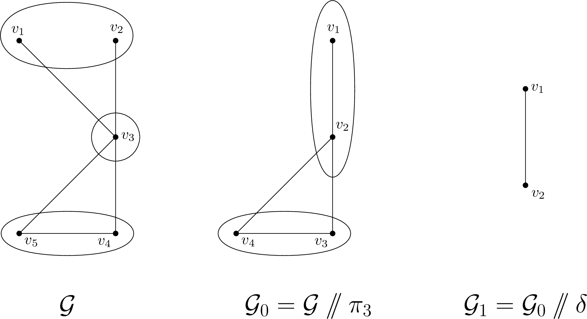
For example, consider the 2-chain $\chi\left(\mathcal{V}_{5}\right)=\left\{\pi_{2},\pi_{3}\right\}$ with

\pi_{2}\left(\mathcal{V}_{5}\right)=\left\{\underbrace{\left\{v_{1},v_{2},v_{3}\right\}}_{C_{1}},\underbrace{\left\{v_{4},v_{5}\right\}}_{C_{2}}\right\},\mbox{ and }\pi_{3}\left(\mathcal{V}_{5}\right)=\left\{\underbrace{\left\{v_{1},v_{2}\right\}}_{C_{1}},\underbrace{\left\{v_{3}\right\}}_{C_{2}},\underbrace{\left\{v_{4},v_{5}\right\}}_{C_{3}}\right\}.

We have $C_{1}\left(\pi_{3}\right),C_{2}\left(\pi_{3}\right)\subseteq C_{1}\left(\pi_{2}\right)$ and $C_{3}\left(\pi_{3}\right)\subseteq C_{2}\left(\pi_{2}\right)$ , therefore, $\pi_{3}<\pi_{2}$ . We can then construct the coarsening sequence $\Delta\left(\chi\right)=\delta\left(\pi_{3},\pi_{2}\right)$ with $\delta\left(\pi_{3},\pi_{2}\right)=\{\underbrace{\left\{1,2\right\}}_{C_{1}},\underbrace{\left\{3\right\}}_{C_{2}}\}$ . The resulting graph contraction sequence is presented in Figure 3.

3.2 Edge Contractions

Graph contractions are defined over vertex partitions. However, there is also an edge-based approach to perform graph contractions.

Definition 8 (edge contraction partition).

Consider a graph $\mathcal{G}$ and an edge contraction set $\mathcal{E}_{cs}\subset\mathcal{E}(\mathcal{G})$ with $|\mathcal{E}_{cs}|=n-r$ . Then we define the edge contraction partition $\pi_{c}\left(\mathcal{G},\mathcal{E}_{cs}\right)$ as the connected components partition of the graph $\mathcal{G}_{c}\left(\mathcal{G},\mathcal{E}_{cs}\right)=\left(\mathcal{V}\left(\mathcal{G}\right),\mathcal{E}_{cs}\right)$ , i.e., $\pi_{c}\left(\mathcal{G},\mathcal{E}_{cs}\right)=\pi_{cc}\left(\mathcal{G}_{c}\left(\mathcal{G},\mathcal{E}_{cs}\right)\right)$ . The set of all edge contraction sets of cardinality $p$ is defined as $\Xi_{p}\left(\mathcal{G}\right)\triangleq\left\{\mathcal{E}_{cs}\subset\mathcal{E}\left(\mathcal{G}\right)|\left|\mathcal{E}_{cs}\right|=p\right\}$ .

With the edge contraction partition definition we can define an edge-based graph contraction.

Definition 9 (edge-based graph contraction).

Consider a graph $\mathcal{G}$ and an edge contraction set $\mathcal{E}_{cs}\in\Xi_{n-r}\left(\mathcal{G}\right)$ for $r<n$ . Then the edge-based contraction is defined as the contraction over the edge contraction partition, i.e., $\mathcal{G}\sslash\mathcal{E}_{cs}=\mathcal{G}\sslash\pi_{c}\left(\mathcal{G},\mathcal{E}_{cs}\right)$ .

In this work we find that a class of edge-matching contractions has interlacing properties.

Definition 10 (edge-matching contraction).

Consider a graph $\mathcal{G}$ and an edge contraction set $\mathcal{E}_{cs}\in\Xi_{n-r}\left(\mathcal{G}\right)$ for $r<n$ . Then $\mathcal{G}\sslash\mathcal{E}_{cs}$ is an edge-matching contraction if there is one-to-one correspondence between $\mathcal{E}\left(\mathcal{G}\right)\backslash\mathcal{E}_{cs}$ and $\mathcal{E}\left(\mathcal{G}\sslash\mathcal{E}_{cs}\right)$ .

A graph contraction cannot create new edges, therefore, edge-matching (Definition 10) is equivalent to $\left|\mathcal{E}\left(\mathcal{G}\right)\backslash\mathcal{E}_{cs}\right|=\left|\mathcal{E}\left(\mathcal{G}\sslash\mathcal{E}_{cs}\right)\right|$ .

Proposition 5.

Consider a graph $\mathcal{G}$ and an edge contraction set $\mathcal{E}_{cs}\in\Xi_{n-r}\left(\mathcal{G}\right)$ . Then if $\mathcal{G}\sslash\mathcal{E}_{cs}$ is cycle-invariant (Definition 4) it is also edge-matching (Definition 10).

Proof.

If $\mathcal{G}\sslash\mathcal{E}_{cs}$ is cycle-invariant then from Definition 4 the edges in $\mathcal{E}_{cs}$ are not part of any cycle of $\mathcal{G}$ . Therefore, the contraction does not map any two edges in $\mathcal{E}\left(\mathcal{G}\right)\backslash\mathcal{E}_{cs}$ to a single edge in $\mathcal{E}\left(\mathcal{G}\sslash\mathcal{E}_{cs}\right)$ , otherwise they would have been part of a cycle with an edge in $\mathcal{E}_{cs}$ , and we obtain that $\left|\mathcal{E}\left(\mathcal{G}\right)\backslash\mathcal{E}_{cs}\right|=\left|\mathcal{E}\left(\mathcal{G}\sslash\mathcal{E}_{cs}\right)\right|$ .∎

Proposition 6.

Consider a graph $\mathcal{G}$ and a node $v\in\mathcal{V}\left(G\right)$ , and let $\pi_{cc}\left(\mathcal{G}\backslash v\right)$ be the connected component partition of $\mathcal{G}\backslash v$ , then for $C_{i}\in\pi_{cc}\left(\mathcal{G}\backslash v\right)$ and $\mathcal{E}_{cs}=\mathcal{E}\left(\mathcal{G}\left[C_{i}\cup v\right]\right)$ , the contraction $\mathcal{G}\sslash\mathcal{E}_{cs}$ is node-removal equivalent (Definition 3) with $\mathcal{V}_{S}=C_{i}$ , and is also edge-matching (Definition 10).

Proof.

Since $C_{i}$ is a connected component of $\mathcal{G}\backslash\mathcal{E}\left(\mathcal{G}\left[\mathcal{N}_{v}\cup v\right]\right)$ then $v$ is the only node in any path between $C_{i}$ and $\mathcal{V}\left(\mathcal{G}\right)\backslash\left\{C_{i}\cup v\right\}$ , therefore, by choosing $\mathcal{V}_{S}=C_{i}$ the graph $\mathcal{G}\backslash C_{i}$ removes all edges $\mathcal{E}\left(\mathcal{G}\left[C_{i}\right]\right)$ and all edges connecting $C_{i}$ to $\mathcal{V}\left(\mathcal{G}\right)\backslash C_{i}$ which are the edges between $C_{i}$ and $v$ and we obtain that $\mathcal{G}\backslash C_{i}=\mathcal{G}\sslash\mathcal{E}\left(\mathcal{G}\left[C_{i}\cup v\right]\right)$ , i.e., the contraction $\mathcal{G}\sslash\mathcal{E}_{cs}$ is node-removal equivalent (Definition 3). Furthermore, contracting all edges $\mathcal{E}\left(\mathcal{G}\left[C_{i}\cup v\right]\right)$ does not effect any other edges in $\mathcal{G}$ such that $\left|\mathcal{E}\left(\mathcal{G}\right)\backslash\mathcal{E}_{cs}\right|=\left|\mathcal{E}\left(\mathcal{G}\sslash\mathcal{E}_{cs}\right)\right|$ and we obtain that $\mathcal{G}\sslash\mathcal{E}_{cs}$ is edge-matching.∎

We can choose a subset of tree edges to create a tree-based contraction of a graph.

Definition 11 (tree-based contraction).

For example, the graph contraction $\mathcal{G}\sslash\pi$ presented in Figure 2 can also be performed as an edge-based contraction $\mathcal{G}\sslash\mathcal{E}_{cs}$ with $\mathcal{E}_{cs}=\left\{\left\{v_{1},v_{3}\right\},\left\{v_{2},v_{3}\right\}\right\}$ and a tree-based contraction (Definition 11).

If the contraction edge set is a subset of the edges of a spanning tree, then the contracted tree edges will form a spanning tree of the contracted graph.

Proposition 7.

Consider a graph $\mathcal{G}$ and its spanning tree $\mathcal{T}\in\mathbb{T}\left(\mathcal{G}\right)$ with an edge contraction set $\mathcal{E}_{cs}\in\Xi_{n-r}\left(\mathcal{T}\right)$ . Then $\mathcal{T}\sslash\mathcal{E}_{cs}\in\mathbb{T}\left(\mathcal{G}\sslash\mathcal{E}_{cs}\right)$ , i.e., $\mathcal{T}\sslash\mathcal{E}_{cs}$ is a tree of order $r$ of the contracted graph.

Proof.

A tree of order $n$ has $n-1$ edges, and by contracting $n-r$ tree edges we are left with $\left(n-1\right)-\left(n-r\right)$ edges, such that $\left|\mathcal{E}\left(\mathcal{T}\sslash\mathcal{E}_{cs}\right)\right|=r-1$ . It is left to show that $\mathcal{T}\sslash\mathcal{E}_{cs}\left(\mathcal{T}\right)\subseteq\mathcal{G}\sslash\mathcal{E}_{cs}\left(\mathcal{T}\right)$ . From Lemma 3 we obtain that $\mathcal{T}\sslash\mathcal{E}_{cs}$ is connected, therefore, $\mathcal{T}\sslash\mathcal{E}_{cs}$ is a connected graph of order $r$ with $r-1$ edges, which is a tree of order $r$ . Since $\mathcal{E}_{cs}\left(\mathcal{T}\right)\subseteq\mathcal{E}\left(\mathcal{G}\right)$ we have $\pi_{c}\left(\mathcal{T},\mathcal{E}_{cs}\left(\mathcal{T}\right)\right)=\pi_{c}\left(\mathcal{G},\mathcal{E}_{cs}\left(\mathcal{T}\right)\right)$ , and since $\mathcal{T}=\mathcal{G}\backslash\mathcal{E}\left(\mathcal{C}\right)$ we obtain from the subgraph contraction lemma (Lemma 1) that $\mathcal{T}\sslash\pi_{c}\left(\mathcal{T},\mathcal{E}_{cs}\left(\mathcal{T}\right)\right)\subseteq\mathcal{G}\sslash\pi_{c}\left(\mathcal{T},\mathcal{E}_{cs}\left(\mathcal{T}\right)\right)$ and conclude that $\mathcal{T}\sslash\mathcal{E}_{cs}\left(\mathcal{T}\right)\subseteq\mathcal{G}\sslash\mathcal{E}_{cs}\left(\mathcal{T}\right)$ , and therefore, $\mathcal{T}\sslash\mathcal{E}_{cs}\left(\mathcal{T}\right)\in\mathbb{T}\left(\mathcal{G}\sslash\mathcal{E}_{cs}\right)$ .∎

Proposition 8.

Consider a graph $\mathcal{G}$ and an edge contraction set $\mathcal{E}_{cs}\in\Xi_{n-r}\left(\mathcal{G}\right)$ . Then $\forall\tilde{v}\in\mathcal{V}\left(\mathcal{G}\sslash\mathcal{E}_{cs}\right)$

d_{\tilde{v}}\left(\mathcal{G}\sslash\mathcal{E}_{cs}\right)\leq\left(\sum\limits_{v\in C_{\tilde{v}}\left(\pi\right)}d_{v}\left(\mathcal{G}\right)\right)-2\left(\left|C_{\tilde{v}}\left(\pi\right)\right|-1\right),

(5)

where $\pi=\pi_{c}\left(\mathcal{G},\mathcal{E}_{cs}\right)$ .

Proof.

From Proposition 3 we obtain that $d_{\tilde{v}}\left(\mathcal{G}\sslash\pi\right)=\left|f_{\pi}\left(\mathcal{N}_{C_{\tilde{v}}}\right)\right|$ . We have $\left|f_{\pi}\left(\mathcal{N}_{C_{\tilde{v}}}\right)\right|\leq\left|\mathcal{N}_{C_{\tilde{v}}}\right|$ and since $C_{\tilde{v}}\left(\pi\right)\in\pi_{c}$ is a connected component of $\mathcal{G}$ we get

\displaystyle\left|\mathcal{N}_{C_{\tilde{v}}}\right|

\displaystyle\leq\left(\sum\limits_{v\in C_{\tilde{v}}\left(\pi\right)}d_{v}\left(\mathcal{G}\right)\right)-2\left|\mathcal{E}\left(\mathcal{G}\left[C_{\tilde{v}}\left(\pi\right)\right]\right)\right|.

The number of edges in the cell $\left|\mathcal{E}\left(\mathcal{G}\left[C_{\tilde{v}}\left(\pi\right)\right]\right)\right|$ is at least the number of spanning tree edges, therefore, $\left|\mathcal{E}\left(\mathcal{G}\left[C_{\tilde{v}}\left(\pi\right)\right]\right)\right|\geq\left|C_{\tilde{v}}\left(\pi\right)\right|-1$ , and we obtain that

d_{\tilde{v}}\left(\mathcal{G}\sslash\mathcal{E}_{cs}\right)\leq\left(\sum\limits_{v\in C_{\tilde{v}}\left(\pi\right)}d_{v}\left(\mathcal{G}\right)\right)-2\left(\left|C_{\tilde{v}}\left(\pi\right)\right|-1\right),

completing the proof.∎

Corollary 2.

Consider a graph $\mathcal{G}$ and an edge contraction set $\mathcal{E}_{cs}\in\Xi_{n-r}\left(\mathcal{G}\right)$ for $r<n$ . Then if $\mathcal{G}\sslash\mathcal{E}_{cs}$ is cycle-invariant (Definition 3) then $\forall\tilde{v}\in\mathcal{V}\left(\mathcal{G}\sslash\mathcal{E}_{cs}\right)$ ,

d_{\tilde{v}}\left(\mathcal{G}\sslash\mathcal{E}_{cs}\right)=\left(\sum\limits_{v\in C_{\tilde{v}}\left(\pi\right)}d_{v}\left(\mathcal{G}\right)\right)-2\left(\left|C_{\tilde{v}}\left(\pi\right)\right|-1\right),

(6)

where $\pi=\pi_{c}\left(\mathcal{G},\mathcal{E}_{cs}\right)$ .

Proof.

Since $\forall\tilde{v}\in\mathcal{V}\left(\mathcal{G}\sslash\mathcal{E}_{cs}\right)$ $C_{\tilde{v}}\left(\pi\right)$ is a connected component of $\mathcal{G}$ , and $\mathcal{G}\sslash\mathcal{E}_{cs}$ is cycle-invariant then $\left|f_{\pi}\left(\mathcal{N}_{C_{\tilde{v}}}\right)\right|=\left|\mathcal{N}_{C_{\tilde{v}}}\right|$ and $\mathcal{G}\left[C_{\tilde{v}}\left(\pi\right)\right]$ is a tree of order $\left|C_{\tilde{v}}\left(\pi\right)\right|$ , such that from Proposition 3 we obtain that

d_{\tilde{v}}\left(\mathcal{G}\sslash\mathcal{E}_{cs}\right)=\left(\sum\limits_{v\in C_{\tilde{v}}\left(\pi\right)}d_{v}\left(\mathcal{G}\right)\right)-2\left(\left|C_{\tilde{v}}\left(\pi\right)\right|-1\right).

∎

Corollary 3.

If a graph $\mathcal{G}$ is a tree then $\mathcal{G}\sslash\mathcal{E}_{cs}$ is edge-matching for any $\mathcal{E}_{cs}\in\Xi_{n-r}\left(\mathcal{G}\right)$ .

Proof.

If $\mathcal{G}$ is a tree then $\mathcal{G}\sslash\mathcal{E}_{cs}$ is cycle-invariant for any $\mathcal{E}_{cs}\in\Xi_{n-r}\left(\mathcal{G}\right)$ and from Proposition 5 we obtain that $\mathcal{G}\sslash\mathcal{E}_{cs}$ is edge-matching.∎

Trees and cycle-completing edges are the building blocks of any connected graph, and this tree and co-tree structure is described by the Tucker representation [16, p.113].

Definition 12 (Tucker representation).

Consider a graph $\mathcal{G}$ and its spanning tree $\mathcal{T}\in\mathbb{T}\left(\mathcal{G}\right)$ with co-tree $\mathcal{C}\left(\mathcal{T}\right)$ , with arbitrary head and tail assigned to the end-nodes of each edge in $\mathcal{E}\left(\mathcal{G}\right)$ . For each edge $\epsilon_{j}\in\mathcal{E}\left(\mathcal{C}\right)$ there is a path from head to tail in $\mathcal{T}$ , and we define a corresponding signed path vector $t_{j}\in\mathbb{R}^{\left|\mathcal{E}\left(\mathcal{T}\right)\right|}$ , $\left[t_{j}\right]_{k}=1$ if $\epsilon_{k}\left(\mathcal{T}\right)$ (with the assigned head and tail) is along the path, $\left[t_{j}\right]_{k}=-1$ if $\epsilon_{k}\left(\mathcal{T}\right)$ is opposite to the path, and $\left[t_{j}\right]_{k}=0$ otherwise. The Tucker representation of the co-tree is then the matrix $T_{\left(\mathcal{T},\mathcal{C}\right)}\in\mathbb{R}^{\left|\mathcal{E}\left(\mathcal{T}\right)\right|\times\left|\mathcal{E}\left(\mathcal{C}\right)\right|}$ where the $j$ th column of $T_{\left(\mathcal{T},\mathcal{C}\right)}$ is the signed path vector $t_{j}\in\mathbb{R}^{\left|\mathcal{E}\left(\mathcal{T}\right)\right|}$ of the corresponding edge $\epsilon_{j}\in\mathcal{E}\left(\mathcal{C}\right)$ .

Proposition 9.

Consider a graph $\mathcal{G}$ and an edge contraction set $\mathcal{E}_{cs}\in\Xi_{n-r}\left(\mathcal{G}\right)$ for $r<n$ , and let $\mathcal{T}\in\mathbb{T}\left(\mathcal{G}\right)$ . Then $\mathcal{G}\sslash\mathcal{E}_{cs}$ is cycle-invariant (Definition 4) if and only if $\mathcal{E}_{cs}\subseteq\mathcal{E}\left(\mathcal{T}\right)$ and the corresponding rows of $T_{\left(\mathcal{T},\mathcal{C}\right)}$ are all zeros.

Proof.

If $\mathcal{G}\sslash\mathcal{E}_{cs}$ is cycle-invariant then from Definition 4 the edges in $\mathcal{E}_{cs}$ are not part of any cycle of $\mathcal{G}$ , therefore, $\mathcal{E}_{cs}\subseteq\mathcal{E}\left(\mathcal{T}\right)$ for any $\mathcal{T}\in\mathbb{T}\left(\mathcal{G}\right)$ . If $\epsilon\in\mathcal{E}\left(\mathcal{T}\right)$ is not part of any cycle in $\mathcal{G}$ then form the Tucker representation (Definition 12) we get that the corresponding row of $T_{\left(\mathcal{T},\mathcal{C}\right)}$ is all zeros.

If $\mathcal{E}_{cs}\subseteq\mathcal{E}\left(\mathcal{T}\right)$ and the corresponding rows of $T_{\left(\mathcal{T},\mathcal{C}\right)}$ are all zeros, then the edges in $\mathcal{E}_{cs}$ are not part of any cycle in $\mathcal{G}$ , such that the tree-based contraction (Definition 11) $\mathcal{G}\sslash\mathcal{E}_{cs}$ is cycle-invariant.∎

4 Interlacing Graph Contractions

The general interlacing graph reduction problem (Problem 1) is combinatorial hard. If we restrict the class of reduced-order graphs to graph contractions then we get the following interlacing graph contraction problem.

Problem 2 (interlacing graph contraction).

Consider a graph $\mathcal{G}$ and a real symmetric graph matrix $M\left(\mathcal{G}\right)\in\mathbb{R}^{n\times n}$ . Then given $r<n$ find $\pi\in\Pi_{r}\left(\mathcal{G}\right)$ such that $\mathcal{G}\sslash\pi\propto_{M}\mathcal{G}$ .

The number of $r$ -partitions is $\left|\Pi_{r}\left(\mathcal{G}\right)\right|=S\left(n,r\right)$ where

S\left(n,r\right)=\sum\limits_{k=1}^{r}\left(-1\right)^{r-k}\frac{k^{n}}{k!\left(r-k\right)!},

is the Stirling number of the second kind [11, p.18], which for $r\ll n$ is asymptotically $S\left(n,r\right)\sim\frac{r^{n}}{r!}$ . If we restrict the problem to edge-based contractions then the number of partitions is the number of $n-r$ edge contractions is $\left|\Xi_{n-r}\left(\mathcal{G}\right)\right|=\left(\begin{array}[]{c}m\\ n-r\end{array}\right)$ where $m=\left|\mathcal{E}\left(\mathcal{G}\right)\right|$ . Finding an interlacing contraction is, therefore, combinatorial hard as well and in the following section we show how cycle-invariant and node-removal equivalent contractions have associated subspaces required by Theorem 3 and lead to interlacing graphs.

Consider a graph $\mathcal{G}=\left(\mathcal{V},\mathcal{E}\right)$ of order $n$ and an $r$ -partition $\pi\in\Pi_{r}\left(\mathcal{G}\right)$ and consider a subset $\mathcal{V}_{S}\subset\mathcal{V}\left(\mathcal{G}\right)$ , $\left|\mathcal{V}_{S}\right|=n-r$ for $r<n$ . Then we define the following subspaces of dimension $r$ . The partition subspace $\mathcal{F}_{\pi}\subseteq\mathbb{R}^{n}$ is the space of all vectors in $\mathbb{R}^{n}$ such that variables with indexes in the same partition cell are equal,

\mathcal{F}_{\pi}\triangleq\left\{x\in\mathbb{R}^{n}|x_{j}=x_{k},\forall j,k\in C_{i}\left(\pi\right),\forall i\in\left[1,r\right]\right\},

(7)

and the corresponding partition mapping $p_{\mathcal{F}_{\pi}}\left(\tilde{x}\right):\mathbb{R}^{r}\rightarrow\mathbb{R}^{n}$ ,

\left[p_{\mathcal{F}_{\pi}}\left(\tilde{x}\right)\right]_{k}=\left\{\tilde{x}_{i}|k\in C_{i}\left(\pi\right)\right\}.

(8)

We define the anti-partition subspace $\tilde{\mathcal{F}}_{\pi}\subseteq\mathbb{R}^{n}$ such that for $x\in\tilde{\mathcal{F}}_{\pi}$ the sum of all vector variables in non-singleton partition cells is zero

\tilde{\mathcal{F}}_{\pi}\triangleq\left\{x\in\mathbb{R}^{n}|x_{v_{j}\left(C_{i}\left(\pi\right)\right)}=-\frac{x_{v_{1}\left(C_{i}\left(\pi\right)\right)}}{\left|C_{i}\left(\pi\right)\right|-1},\begin{array}[]{c}\forall i\in\left[1,r\right],\text{$\left|C_{i}\left(\pi\right)\right|>1$}\\ \forall j\in\left[2,\left|C_{i}\left(\pi\right)\right|\right]\end{array}\right\},

(9)

and the corresponding anti-partition mapping, $p_{\tilde{\mathcal{F}}_{\pi}}\left(\tilde{x}\right):\mathbb{R}^{r}\rightarrow\mathbb{R}^{n}$ ,

\left[p_{\tilde{\mathcal{F}}_{\pi}}\left(\tilde{x}\right)\right]_{k}=\begin{cases}\tilde{x}_{k}&k=v_{1}\left(C_{i}\left(\pi\right)\right)\\ -\frac{\tilde{x}_{k}}{\left|C_{i}\left(\pi\right)\right|-1}&k=v_{j}\left(C_{i}\left(\pi\right)\right),j\geq 2\end{cases},

(10)

where $v_{j}\left(C_{i}\left(\pi\right)\right)$ denotes the j’th node of the i’th partition cell.

The node-removal subspace, $\mathcal{F}_{\mathcal{V}_{S}}\subseteq\mathbb{R}^{n}$ , is defined as

\mathcal{F}_{\mathcal{V}_{S}}\triangleq\left\{x\in\mathbb{R}^{n}|x_{i}=0,i\in\mathcal{V}_{S}\right\},

(11)

and the corresponding node-removal mapping $p_{\mathcal{F}_{\mathcal{V}_{S}}}\left(\tilde{x}\right):\mathbb{R}^{r}\rightarrow\mathbb{R}^{n}$ ,

\left[p_{\mathcal{F}_{\mathcal{V}_{S}}}\left(\tilde{x}\right)\right]_{k}=\begin{cases}\tilde{x}_{k}&k\notin\mathcal{V}_{S}\\ 0&o.w.\end{cases}.

(12)

Proposition 10.

Consider a graph $\mathcal{G}$ and an edge-matching and node-removal equivalent contraction $\mathcal{G}\sslash\mathcal{E}_{cs}$ (Definitions 10&8) with $\mathcal{E}_{cs}\in\Xi_{n-r}\left(\mathcal{G}\right)$ for $r<n$ . Then for $\tilde{x}\in\mathbb{R}^{r}$ we have

R\left(L\left(\mathcal{G}\right),p_{\mathcal{F}_{\pi}}\left(\tilde{x}\right)\right)\leq R\left(L\left(\mathcal{G}\sslash\mathcal{E}_{cs}\right),\tilde{x}\right),

and

R\left(L\left(\mathcal{G}\right),p_{\mathcal{F}_{\mathcal{V}_{S}}}\left(\tilde{x}\right)\right)\geq R\left(L\left(\mathcal{G}\sslash\mathcal{E}_{cs}\right),\tilde{x}\right).

Proof.

Let $x=p_{\mathcal{F}_{\pi}}\left(\tilde{x}\right)$ for $\tilde{x}\in\mathbb{R}^{r}$ . The Rayleigh quotients of the Laplacian takes the form [3]

R\left(L\left(\mathcal{G}\right),x\right)=\frac{\sum\limits_{\left\{u,v\right\}\in\mathcal{E}\left(\mathcal{G}\right)}\left(x_{v}-x_{u}\right)^{2}}{\sum\limits_{v\in\mathcal{V}\left(\mathcal{G}\right)}x_{v}^{2}}.

Separating the edges to $\mathcal{E}_{cs}$ and $\mathcal{E}\backslash\mathcal{E}_{cs}$ , the sum $\sum\limits_{\left\{u,v\right\}\in\mathcal{E}\left(\mathcal{G}\right)}\left(x_{v}-x_{u}\right)^{2}$ can be written as

\sum\limits_{\left\{u,v\right\}\in\mathcal{E}\left(\mathcal{G}\right)}\left(x_{v}-x_{u}\right)^{2}=\sum\limits_{\left\{u,v\right\}\in\mathcal{E}\left(\mathcal{G}\right)\backslash\mathcal{E}_{cs}}\left(x_{u}-x_{v}\right)^{2}+\sum\limits_{\left\{u,v\right\}\in\mathcal{E}_{cs}}\left(x_{u}-x_{v}\right)^{2}.

Therefore, if $x\in\mathcal{F}_{\pi}$ and $\left\{u,v\right\}\in\mathcal{E}_{cs}$ then $\sum\limits_{\left\{u,v\right\}\in\mathcal{E}_{cs}}\left(x_{u}-x_{v}\right)^{2}=0$ and

\sum\limits_{\left\{u,v\right\}\in\mathcal{E}}\left(x_{v}-x_{u}\right)^{2}=\sum\limits_{\left\{u,v\right\}\in\mathcal{E}\backslash\mathcal{E}_{cs}}\left(x_{u}-x_{v}\right)^{2}.

Since $\mathcal{G}\sslash\mathcal{E}_{cs}$ is edge-matching (Definition 10) there is one-to-one correspondence between $\mathcal{E}\left(\mathcal{G}\right)\backslash\mathcal{E}_{cs}$ and $\mathcal{E}\left(\mathcal{G}\sslash\mathcal{E}_{cs}\right)$ (Proposition 5), and substituting the partition lifting $x=p_{\mathcal{F}_{\pi}}\left(\tilde{x}\right)$ (Eq. (8)) we get

\sum\limits_{\left\{u,v\right\}\in\mathcal{E}\backslash\mathcal{E}_{cs}}\left(x_{u}-x_{v}\right)^{2}=\sum\limits_{\left\{u,v\right\}\in\mathcal{E}\left(\mathcal{G}\sslash\mathcal{E}_{cs}\right)}\left(\tilde{x}_{u}-\tilde{x}_{v}\right)^{2}.

Rearranging the sums $\sum\limits_{v\in\mathcal{V}}x_{v}^{2}$ over the vertices of each partition cell and substituting the partition lifting $x=p_{\mathcal{F}_{\pi}}\left(\tilde{x}\right)$ (Eq. (8)) we get,

	$\displaystyle\sum\limits_{v\in\mathcal{V}\left(\mathcal{G}\right)}x_{v}^{2}$	$\displaystyle=\sum_{i=1}^{r}\sum\limits_{v\in C_{i}\left(\pi\right)}x_{v}^{2}$
		$\displaystyle=\sum\limits_{u\in\mathcal{V}\left(\mathcal{G}\sslash\mathcal{E}_{cs}\right)}\tilde{x}_{u}^{2}\left\|C_{u}\left(\pi\right)\right\|,$

The Rayleigh quotients of the Laplacian is then

R\left(L\left(\mathcal{G}\right),p_{\mathcal{F}_{\pi}}\left(\tilde{x}\right)\right)=\frac{\sum\limits_{\left\{u,v\right\}\in\mathcal{E}\left(\mathcal{G}\sslash\mathcal{E}_{cs}\right)}\left(\tilde{x}_{u}-\tilde{x}_{v}\right)^{2}}{\sum\limits_{u\in\mathcal{V}\left(\mathcal{G}\sslash\mathcal{E}_{cs}\right)}\tilde{x}_{u}^{2}\left|C_{u}\left(\pi\right)\right|},

and we have $\left|C_{i}\left(\pi\right)\right|\geq 1$ , therefore,

	$\displaystyle R\left(L\left(\mathcal{G}\right),p_{\mathcal{F}_{\pi}}\left(\tilde{x}\right)\right)$	$\displaystyle\leq\frac{\sum\limits_{\left\{u,v\right\}\in\mathcal{E}\left(\mathcal{G}\sslash\mathcal{E}_{cs}\right)}\left(\tilde{x}_{u}-\tilde{x}_{v}\right)^{2}}{\sum\limits_{u\in\mathcal{V}\left(\mathcal{G}\sslash\mathcal{E}_{cs}\right)}\tilde{x}_{u}^{2}}$
		$\displaystyle=R\left(L\left(\mathcal{G}\sslash\mathcal{E}_{cs}\right),\tilde{x}\right).$

If $\mathcal{G}\sslash\mathcal{E}_{cs}$ is node-removal equivalent (Definition 3) then by substituting the node-removal lifting $x=p_{\mathcal{F}_{\mathcal{V}_{S}}}\left(\tilde{x}\right)$ (Eq. (8)) we get

\sum\limits_{\left\{u,v\right\}\in\mathcal{E}\backslash\mathcal{E}_{cs}}\left(x_{u}-x_{v}\right)^{2}=\sum\limits_{\left\{u,v\right\}\in\mathcal{E}\left(\mathcal{G}\sslash\mathcal{E}_{cs}\right)}\left(\tilde{x}_{u}-\tilde{x}_{v}\right)^{2}

and

\sum\limits_{v\in\mathcal{V}\left(\mathcal{G}\right)}x_{v}^{2}=\sum\limits_{u\in\mathcal{V}\left(\mathcal{G}\sslash\mathcal{E}_{cs}\right)}\tilde{x}_{u}^{2},

and we obtain that

	$\displaystyle R\left(L\left(\mathcal{G}\right),p_{\mathcal{F}_{\mathcal{V}_{S}}}\left(\tilde{x}\right)\right)$	$\displaystyle\geq\frac{\sum\limits_{\left\{u,v\right\}\in\mathcal{E}\backslash\mathcal{E}_{cs}}\left(x_{v}-x_{u}\right)^{2}}{\sum\limits_{v\in\mathcal{V}\left(\mathcal{G}\right)}x_{v}^{2}}$
		$\displaystyle=\frac{\sum\limits_{\left\{u,v\right\}\in\mathcal{E}\left(\mathcal{G}\sslash\mathcal{E}_{cs}\right)}\left(\tilde{x}_{u}-\tilde{x}_{v}\right)^{2}}{\sum\limits_{u\in\mathcal{V}\left(\mathcal{G}\sslash\mathcal{E}_{cs}\right)}\tilde{x}_{u}^{2}}$
		$\displaystyle=R\left(L\left(\mathcal{G}\sslash\mathcal{E}_{cs}\right),\tilde{x}\right).$

∎

Proposition 11.

Consider a graph $\mathcal{G}$ and a cycle invariant contraction $\mathcal{G}\sslash\mathcal{E}_{cs}$ (Definition 4) with $\mathcal{E}_{cs}\in\Xi_{n-r}\left(\mathcal{G}\right)$ for $r<n$ . Then for $\tilde{x}\in\mathbb{R}^{r}$ we have

R\left(\mathcal{L}\left(\mathcal{G}\right),p_{\mathcal{F}_{\pi}}\left(\tilde{x}\right)\right)\leq R\left(\mathcal{L}\left(\mathcal{G}\sslash\mathcal{E}_{cs}\right),\tilde{x}\right),

and if $\mathcal{G}\sslash\mathcal{E}_{cs}$ is a single edge contraction with $\mathcal{E}_{cs}=\varepsilon_{cs}$ then

R\left(\mathcal{L}\left(\mathcal{G}\right),p_{\tilde{\mathcal{F}}_{\pi}}\left(\tilde{x}\right)\right)\geq R\left(\mathcal{L}\left(\mathcal{G}\sslash\varepsilon_{cs}\right),\tilde{x}\right).

Proof.

The Rayleigh quotient of the normalized-Laplacian takes the form [3]

R\left(\mathcal{L}\left(\mathcal{G}\right),x\right)=\frac{\sum\limits_{\left\{u,v\right\}\in\mathcal{E}\left(\mathcal{G}\right)}\left(x_{v}-x_{u}\right)^{2}}{\sum\limits_{v\in\mathcal{V}\left(\mathcal{G}\right)}x_{v}^{2}d_{v}\left(\mathcal{G}\right)}.

(13)

Since $\mathcal{G}\sslash\mathcal{E}_{cs}$ is a cycle-invariant contraction it is edge-matching (Proposition 5) and there is one-to-one correspondence between $\mathcal{E}\left(\mathcal{G}\right)\backslash\mathcal{E}_{cs}$ and $\mathcal{E}\left(\mathcal{G}\sslash\mathcal{E}_{cs}\right)$ (Proposition 5), and substituting the partition mapping $x=p_{\mathcal{F}_{\pi}}\left(\tilde{x}\right)$ for $\tilde{x}\in\mathbb{R}^{r}$ (Eq. (8)) we get as in Eq. (4)

	$\displaystyle\sum\limits_{\left\{u,v\right\}\in\mathcal{E}\left(\mathcal{G}\right)}\left(x_{v}-x_{u}\right)^{2}$	$\displaystyle=\sum\limits_{\left\{u,v\right\}\in\mathcal{E}\backslash\mathcal{E}_{cs}}\left(x_{u}-x_{v}\right)^{2}$
		$\displaystyle=\sum\limits_{\left\{u,v\right\}\in\mathcal{E}\left(\mathcal{G}\sslash\mathcal{E}_{cs}\right)}\left(\tilde{x}_{u}-\tilde{x}_{v}\right)^{2}.$

Rearranging the sum $\sum\limits_{v\in\mathcal{V}\left(\mathcal{G}\right)}x_{v}^{2}d_{v}\left(\mathcal{G}\right)$ over the vertices of each partition cell and substituting the partition lifting $x=p_{\mathcal{F}_{\pi}}\left(\tilde{x}\right)$ (Eq. (8)) we get,

	$\displaystyle\sum\limits_{v\in\mathcal{V}\left(\mathcal{G}\right)}x_{v}^{2}d_{v}\left(\mathcal{G}\right)$	$\displaystyle=\sum_{i=1}^{r}\sum\limits_{v\in C_{i}\left(\pi\right)}x_{v}^{2}d_{v}\left(\mathcal{G}\right),$
		$\displaystyle=\sum\limits_{u\in\mathcal{V}\left(\mathcal{G}\sslash\mathcal{E}_{cs}\right)}\tilde{x}_{u}^{2}\left(\sum\limits_{v\in C_{u}\left(\pi\right)}d_{v}\left(\mathcal{G}\right)\right).$

The graph contraction $\mathcal{G}\sslash\mathcal{E}_{cs}$ is cycle-invariant, therefore, from Proposition 2 we have $d_{u}\left(\mathcal{G}\sslash\mathcal{E}_{cs}\right)=\left(\sum\limits_{v\in C_{u}\left(\pi\right)}d_{v}\left(\mathcal{G}\right)\right)-2\left(\left|C_{u}\left(\pi\right)\right|-1\right)$ , and

\sum\limits_{v\in\mathcal{V}\left(\mathcal{G}\right)}x_{v}^{2}d_{v}\left(\mathcal{G}\right)=\sum\limits_{u\in\mathcal{V}\left(\mathcal{G}\sslash\mathcal{E}_{cs}\right)}\tilde{x}_{u}^{2}\left[d_{u}\left(\mathcal{G}\sslash\mathcal{E}_{cs}\right)+2\left(\left|C_{u}\left(\pi\right)\right|-1\right)\right].

The Rayleigh quotients of the normalized-Laplacian (Eq. (13)) is then

R\left(\mathcal{L}\left(\mathcal{G}\right),p_{\mathcal{F}_{\pi}}\left(\tilde{x}\right)\right)=\frac{\sum\limits_{\left\{u,v\right\}\in\mathcal{E}\left(\mathcal{G}\sslash\mathcal{E}_{cs}\right)}\left(\tilde{x}_{u}-\tilde{x}_{v}\right)^{2}}{\sum\limits_{u\in\mathcal{V}\left(\mathcal{G}\sslash\mathcal{E}_{cs}\right)}\tilde{x}_{u}^{2}\left[d_{u}\left(\mathcal{G}\sslash\mathcal{E}_{cs}\right)+2\left(\left|C_{u}\left(\pi\right)\right|-1\right)\right]}.

We have $\left|C_{i}\left(\pi\right)\right|\geq 1$ such that $2\left(\left|C_{i}\left(\pi\right)\right|-1\right)\geq 0$ , therefore,

\displaystyle R\left(\mathcal{L}\left(\mathcal{G}\right),p_{\mathcal{F}_{\pi}}\left(\tilde{x}\right)\right)

\displaystyle\leq\frac{\sum\limits_{\left\{u,v\right\}\in\mathcal{E}\left(\mathcal{G}\sslash\mathcal{E}_{cs}\right)}\left(\tilde{x}_{u}-\tilde{x}_{v}\right)^{2}}{\sum\limits_{u\in\mathcal{V}\left(\mathcal{G}\sslash\mathcal{E}_{cs}\right)}\tilde{x}_{u}^{2}d_{u}\left(\mathcal{G}\sslash\mathcal{E}_{cs}\right)}=R\left(\mathcal{L}\left(\mathcal{G}\sslash\mathcal{E}_{cs}\right),\tilde{x}\right).

Let $\mathcal{G}\sslash\varepsilon_{cs}$ be a cycle-invariant edge contraction with corresponding edge contraction partition $\pi\in\Pi_{n-1}\left(\mathcal{G}\right)$ . For an atom-contraction there is only one non-singlet cell, and without loss of generality we can choose it to be $C_{n-1}\left(\pi\right)=\left\{n-1,n\right\}$ such that the contracted edge is $\varepsilon_{cs}=\left\{x_{n-1},x_{n}\right\}$ , and

R\left(\mathcal{L}\left(\mathcal{G}\right),x\right)=\frac{\sum\limits_{\left\{u,v\right\}\in\mathcal{E}\backslash\mathcal{E}_{cs}}\left(x_{u}-x_{v}\right)^{2}+\left(x_{n-1}-x_{n}\right)^{2}}{\sum\limits_{v=1}^{n-2}x_{v}^{2}d_{v}\left(\mathcal{G}\right)+x_{n-1}^{2}d_{n-1}\left(\mathcal{G}\right)+x_{n}^{2}d_{n}\left(\mathcal{G}\right)}.

For this atom-contraction, we have the anti-partition space $\tilde{\mathcal{F}}_{\pi}=\left\{x\in\mathbb{R}^{n}\,|x_{n-1}=-x_{n}\right\}$ (Eq. (9)) and anti-partition mapping $p_{\tilde{\mathcal{F}}_{\pi}}\left(\tilde{x}\right):\mathbb{R}^{n-1}\rightarrow\mathbb{R}^{n}$ is (Eq. (10))

\left[p_{\tilde{\mathcal{F}}_{\pi}}\left(\tilde{x}\right)\right]_{k}=\begin{cases}\tilde{x}_{k}&k\leq n-1\\ -\tilde{x}_{n-1}&k=n\end{cases},

such that

R\left(\mathcal{L}\left(\mathcal{G}\right),p_{\tilde{\mathcal{F}}_{\pi}}\left(\tilde{x}\right)\right)=\frac{\sum\limits_{\left\{u,v\right\}\in\mathcal{E}\backslash\mathcal{E}_{cs}}\left(\tilde{x}_{u}-\tilde{x}_{v}\right)^{2}+4\tilde{x}_{n-1}^{2}}{\sum\limits_{v=1}^{n-2}\tilde{x}_{v}^{2}d_{v}\left(\mathcal{G}\right)+\tilde{x}_{n-1}^{2}\left(d_{n-1}\left(\mathcal{G}\right)+d_{n}\left(\mathcal{G}\right)\right)}.

There is one-to-one correspondence between $\mathcal{E}\left(\mathcal{G}\right)\backslash\varepsilon_{cs}$ and $\mathcal{E}\left(\mathcal{G}\sslash\varepsilon_{cs}\right)$ (Proposition 5), therefore, $\sum\limits_{\left\{u,v\right\}\in\mathcal{E}\backslash\mathcal{E}_{cs}}\left(\tilde{x}_{u}-\tilde{x}_{v}\right)^{2}=\sum\limits_{\left\{u,v\right\}\in\mathcal{E}\left(\mathcal{G}\sslash\varepsilon_{cs}\right)}\left(\tilde{x}_{u}-\tilde{x}_{v}\right)^{2}$ , and from Proposition 2 we get

d_{v}\left(\mathcal{G}\sslash\varepsilon_{cs}\right)=\begin{cases}d_{v}\left(\mathcal{G}\right)&v\leq n-2\\ d_{n-1}\left(\mathcal{G}\right)+d_{n}\left(\mathcal{G}\right)-2&v=n-1\end{cases},

such that

	$\displaystyle R\left(\mathcal{L}\left(\mathcal{G}\right),p_{\tilde{\mathcal{F}}_{\pi}}\left(\tilde{x}\right)\right)$	$\displaystyle=\frac{\sum\limits_{\left\{u,v\right\}\in\mathcal{E}\left(\mathcal{G}\sslash\varepsilon_{cs}\right)}\left(\tilde{x}_{u}-\tilde{x}_{v}\right)^{2}+4\tilde{x}_{n-1}^{2}}{\sum\limits_{v\in\mathcal{V}\left(\mathcal{G}\sslash\varepsilon_{cs}\right)}\tilde{x}_{v}^{2}d_{v}\left(\mathcal{G}\sslash\varepsilon_{cs}\right)+2\tilde{x}_{n-1}^{2}}$
		$\displaystyle=R\left(\mathcal{L}\left(\mathcal{G}\sslash\varepsilon_{cs}\right),\tilde{x}\right)\frac{1+\frac{4\tilde{x}_{n-1}^{2}}{\sum\limits_{\left\{u,v\right\}\in\mathcal{E}\left(\mathcal{G}\sslash\varepsilon_{cs}\right)}\left(\tilde{x}_{u}-\tilde{x}_{v}\right)^{2}}}{1+\frac{2\tilde{x}_{n-1}^{2}}{\sum\limits_{v\in\mathcal{V}\left(\mathcal{G}\sslash\varepsilon_{cs}\right)}\tilde{x}_{v}^{2}d_{v}\left(\mathcal{G}\sslash\varepsilon_{cs}\right)}}.$

For any $\mathcal{G}$ we have $R\left(\mathcal{L}\left(\mathcal{G}\right),x\right)\leq 2$ [17], therefore,

\sum\limits_{\left\{u,v\right\}\in\mathcal{E}\left(\mathcal{G}\sslash\varepsilon_{cs}\right)}\left(\tilde{x}_{u}-\tilde{x}_{v}\right)^{2}\leq 2\sum\limits_{v\in\mathcal{V}\left(\mathcal{G}\sslash\varepsilon_{cs}\right)}\tilde{x}_{v}^{2}d_{v}\left(\mathcal{G}\sslash\varepsilon_{cs}\right)

and

\frac{1+\frac{4\tilde{x}_{n-1}^{2}}{\sum\limits_{\left\{u,v\right\}\in\mathcal{E}\left(\mathcal{G}\sslash\varepsilon_{cs}\right)}\left(\tilde{x}_{u}-\tilde{x}_{v}\right)^{2}}}{1+\frac{2\tilde{x}_{n-1}^{2}}{\sum\limits_{v\in\mathcal{V}\left(\mathcal{G}\sslash\varepsilon_{cs}\right)}\tilde{x}_{v}^{2}d_{v}\left(\mathcal{G}\sslash\varepsilon_{cs}\right)}}\geq 1,

and we obtain that $R\left(\mathcal{L}\left(\mathcal{G}\right),p_{\tilde{\mathcal{F}}_{\pi}}\left(\tilde{x}\right)\right)\geq R\left(\mathcal{L}\left(\mathcal{G}\sslash\varepsilon_{cs}\right),\tilde{x}\right)$ for any cycle invariant single edge contraction.∎

The only graph contraction interlacing result known to the authors has been presented by Chen et. al. [3]:

Theorem 4 (normalized-Laplacian interlacing disjoint neighborhood contraction).

Consider a graph $\mathcal{G}$ and two vetices $u,v\in\mathcal{V}\left(\mathcal{G}\right)$ with corresponding partition $\pi\in\Pi_{n-1}\left(\mathcal{G}\right)$ with only one non-singlet cell $C_{n-1}\left(\pi\right)=\left\{u,v\right\}$ . Then if $u,v$ have disjoint neighborhoods, i.e., $\mathcal{N}_{u}\left(\mathcal{G}\right)\cap\left\{\mathcal{N}_{v}\left(\mathcal{G}\right)\cup v\right\}=\varnothing$ , the atom contraction is normalized-Laplacian interlacing, i.e., $\mathcal{G}\sslash\pi\propto_{\mathcal{L}}\mathcal{G}$ .

Proof.

The proof is given in [3] and is based on a sequence of min-max ineuqalities and the Courant–Fischer theorem (Theorem 2). In the perspective of this work, Theorem 4 can be proven based on Theorem 3 as follows: Let $\mathcal{G}\sslash\pi$ be an atom contraction with $C_{n-1}\left(\pi\right)=\left\{u,v\right\}$ and $\mathcal{N}_{u}\left(\mathcal{G}\right)\cap\left\{\mathcal{N}_{v}\left(\mathcal{G}\right)\cup v\right\}=\varnothing$ . We notice that if $\mathcal{N}_{u}\left(\mathcal{G}\right)\cap\left\{\mathcal{N}_{v}\left(\mathcal{G}\right)\cup v\right\}=\varnothing$ then $\mathcal{G}\sslash\pi$ is edge-matching (Definition 10). Similar to Proposition 11 it can then be shown that $R\left(\mathcal{L}\left(\mathcal{G}\right),p_{\mathcal{F}_{\pi}}\left(x\right)\right)\leq R\left(\mathcal{L}\left(\mathcal{G}\sslash\pi\right),x\right)$ and $R\left(\mathcal{L}\left(\mathcal{G}\right),p_{\tilde{\mathcal{F}}_{\pi}}\left(\tilde{x}\right)\right)\geq R\left(L\left(\mathcal{G}\sslash\pi\right),x\right)$ , therefore, from Theorem 3 with $\mathcal{A}\equiv\mathcal{F}_{\pi}$ and $\mathcal{B}\equiv\tilde{\mathcal{F}}_{\pi}$ we then get that $\mathcal{G}\sslash\pi\propto_{\mathcal{L}}\mathcal{G}$ . ∎

In this study, based on Theorem 3, we derive two interlacing theorems, Laplacian interlacing for node-removal equivalent edge-matching contractions (Theorem 5) and normalized Laplacian interlacing for cycle-invariant contractions (Theorem 6).

Theorem 5 (Laplacian interlacing node-removal equivalent contraction).

Consider a graph $\mathcal{G}$ and an edge contraction set $\mathcal{E}_{cs}\in\Xi_{n-r}\left(\mathcal{G}\right)$ for $r<n$ . If $\mathcal{G}\sslash\mathcal{E}_{cs}$ is edge-matching (Definition 10) and node-removal equivalent (Definition 3) then $\mathcal{G}\sslash\mathcal{E}_{cs}\propto_{L}\mathcal{G}$ .

Proof.

The contraction $\mathcal{G}\sslash\mathcal{E}_{cs}$ is edge-matching and node-removal equivalent such that from Proposition 10 we have $R\left(L\left(\mathcal{G}\right),p_{\mathcal{F}_{\pi}}\left(x\right)\right)\leq R\left(L\left(\mathcal{G}\sslash\mathcal{E}_{cs}\right),x\right)$ and $R\left(L\left(\mathcal{G}\right),p_{\mathcal{F}_{\mathcal{V}_{S}}}\left(x\right)\right)\geq R\left(L\left(\mathcal{G}\sslash\mathcal{E}_{cs}\right),x\right)$ . Therefore, from Theorem 3 with $\mathcal{A}\equiv\mathcal{F}_{\pi}$ and $\mathcal{B}\equiv\mathcal{F}_{\mathcal{V}}$ we then get that $\mathcal{G}\sslash\mathcal{E}_{cs}\propto_{L}\mathcal{G}$ .∎

Theorem 6 (normalized-Laplacian interlacing cycle-invariant contraction).

Consider a graph $\mathcal{G}$ and an edge contraction set $\mathcal{E}_{cs}\in\Xi_{n-r}\left(\mathcal{G}\right)$ for $r<n$ . Then if $\mathcal{G}\sslash\mathcal{E}_{cs}$ is cycle-invariant (Definition 3), $\mathcal{G}\sslash\mathcal{E}_{cs}\propto_{\mathcal{L}}\mathcal{G}$ .

Proof.

The graph contraction can be performed by a sequence of atom-contractions (Corollary 1), therefore, it is sufficient to show that the interlacing property holds for a single edge-contraction, i.e., $\mathcal{G}\sslash\epsilon_{cs}\propto_{\mathcal{L}}\mathcal{G}$ where $\epsilon_{cs}$ is a single contracted edge. The interlacing of the sequence will then follow from Proposition 1. Let $\mathcal{G}\sslash\varepsilon_{cs}$ be a cycle-invariant edge contraction with corresponding edge contraction partition $\pi\in\Pi_{n-1}\left(\mathcal{G}\right)$ . Without loss of generality we can label the vertices such that the contracted edge is $\varepsilon_{cs}=\left\{x_{n-1},x_{n}\right\}$ , and the anti-partition space is $\tilde{\mathcal{F}}_{\pi}\left(\tilde{x}\right)=\left\{x\in\mathbb{R}^{n}\,|x_{n-1}=-x_{n}\right\}$ (Eq. (4)). From Proposition 11 we have $R\left(\mathcal{L}\left(\mathcal{G}\right),p_{\mathcal{F}_{\pi}}\left(x\right)\right)\leq R\left(\mathcal{L}\left(\mathcal{G}\sslash\epsilon_{cs}\right),x\right)$ and $R\left(\mathcal{L}\left(\mathcal{G}\right),p_{\tilde{\mathcal{F}}_{\pi}}\left(\tilde{x}\right)\right)\geq R\left(L\left(\mathcal{G}\sslash\varepsilon_{cs}\right),x\right)$ , therefore, from Theorem 3 with $\mathcal{A}\equiv\mathcal{F}_{\pi}$ and $\mathcal{B}\equiv\tilde{\mathcal{F}}_{\pi}$ we then get that $\mathcal{G}\sslash\epsilon_{cs}\propto_{\mathcal{L}}\mathcal{G}$ . By performing the contraction sequence (Proposition 1) we get $\mathcal{G}\sslash\mathcal{E}_{cs}\propto_{\mathcal{L}}\mathcal{G}$ .∎

Corollary 4.

Consider a tree $\mathcal{T}=\left(\mathcal{V},\mathcal{E}\right)$ of order $n$ , and its contraction $\mathcal{T}\sslash\mathcal{E}_{cs}$ for any $\mathcal{E}_{cs}\in\Xi_{n-r}\left(\mathcal{T}\right)$ . Then $\mathcal{T}\sslash\mathcal{E}_{cs}\propto_{\mathcal{L}}\mathcal{T}$ .

Proof.

The contraction $\mathcal{T}\sslash\mathcal{E}_{cs}$ is cycle-invariant for any $\mathcal{E}_{cs}\in\Xi_{n-r}\left(\mathcal{T}\right)$ , therefore, from Theorem 6 we obtain that $\mathcal{T}\sslash\mathcal{E}_{cs}\propto_{\mathcal{L}}\mathcal{T}$ .∎

Theorem 5 and Theorem 6 allow us to try and solve the interlacing graph contraction problem (Problem 2) for normalized Laplacian and Laplacian interlacing by finding a cycle-invariant contraction (Problem 3) or a node-removal equivalent and edge matching contraction (Problem 4) respectively.

Problem 3 (cycle-invariant contraction).

For a graph $\mathcal{G}$ and a given reduction order $r<n$ , find $\mathcal{E}_{cs}\in\Xi_{n-r}\left(\mathcal{G}\right)$ such that $\mathcal{G}\sslash\mathcal{E}_{cs}$ is cycle-invariant (Definition 4).

Problem 4 (node-removal equivalent contraction).

From Proposition 9, we can obtain a cycle-invariant contraction, if exists, from the zero rows of the Tucker representation. A Tucker representation $T_{\left(\mathcal{T},\mathcal{C}\right)}$ can be calculated by finding a spanning tree $\mathcal{T}\in\mathbb{T}\left(\mathcal{G}\right)$ and then finding the path in $\mathcal{T}$ between the end-nodes of each edge of $\mathcal{C}\left(\mathcal{T}\right)$ as described in Algorithm 1. Each path finding operation, e.g., with a depth-first search, is of complexity $\mathcal{O}\left(n\right)$ , and since $\mathcal{O}\left(\left|\mathcal{E}\left(\mathcal{C}\right)\right|\right)=\mathcal{O}\left(\left|\mathcal{E}\left(\mathcal{G}\right)\right|\right)$ the overall complexity of constructing $T_{\left(\mathcal{T},\mathcal{C}\right)}$ is $\mathcal{O}\left(mn\right)$ , where $m=\left|\mathcal{E}\left(\mathcal{G}\right)\right|$ . Therefore, the cycle-invariant contraction algorithm (Algorithm 1) is of complexity $\mathcal{O}\left(mn\right)$ .

From Proposition 6, we can obtain a node-removal equivalent and edge matching contraction, if exists, by first finding for all vertices of $\mathcal{G}$ the connected components partition $\pi_{cc}\left(\mathcal{G}\backslash v\right)$ and then constructing $\mathcal{E}_{cs}$ by choosing from all partitions $\left\{\pi_{cc}\left(\mathcal{G}\backslash v\right)\right\}_{v=1}^{n}$ a subset of cells with a total number of $n-r$ unique nodes (Algorithm 3). Each connected component finding operation, e.g., with a depth-first search, is of complexity $\mathcal{O}\left(n+m\right)$ , and repeated $n$ times, the overall complexity of the algorithm is $\mathcal{O}\left(n^{2}+nm\right)$ .

The feasibility of the cycle-invariant and node-removal equivalent problems requires further study.

Algorithm 1 Cycle-invariant contraction algorithm

Input: graph $\mathcal{G}$ of order $n$ , required reduction order $r$

1.

Find a spanning tree $\mathcal{T}\in\mathbb{T}\left(\mathcal{G}\right)$ and the co-tree $\mathcal{C}\left(\mathcal{T}\right)$ .
2.

Calculate the tucker representation $T_{\left(\mathcal{T},\mathcal{C}\right)}$ (Definition 12).
3.

Choose $n-r$ cycle-invariant edges from the zero rows of $T_{\left(\mathcal{T},\mathcal{C}\right)}$ and obtain $\mathcal{E}_{cs}$ .

Output: $\mathcal{G}_{r}=\mathcal{G}\sslash\mathcal{E}_{cs}$

Algorithm 2 Node-removal equivalent contraction algorithm

Input: graph $\mathcal{G}$ of order $n$ , required reduction order $r$

1.

For $v\in\mathcal{V}\left(\mathcal{G}\right)$ : Calculate $\pi_{cc}\left(\mathcal{G}\backslash v\right)$ , the connected components partition of $\mathcal{G}\backslash v$ .
2.

Choose a subset of cells $\mathcal{S}\subseteq\left\{\pi_{cc}\left(\mathcal{G}\backslash v\right)\right\}_{v=1}^{n}$ with a total number of $n-r$ unique nodes.
3.

Construct $\mathcal{E}_{cs}=\cup_{C_{v}\in\mathcal{S}}\mathcal{E}\left(\mathcal{G}\left[C_{v}\cup v\right]\right)$ .

Output: $\mathcal{G}_{r}=\mathcal{G}\sslash\mathcal{E}_{cs}$

5 Case Studies

As a small-scale normalized Laplacian interlacing example, we consider a graph of order $6$ presented in Figure 4, and we require the reduced graph to be of order $r=4$ . A cycle-invariant graph contraction is then performed with two edges (Figure 4). The resulting reduced graph (Figure 4) has normalized-Laplacian spectra $\left\{\lambda_{k}\left(\mathcal{L}\left(\mathcal{G}_{r}\right)\right)\right\}_{k=1}^{r}$ given in Figure 5 with the upper and lower interlacing bounds $\lambda_{k}\left(\mathcal{L}\left(\mathcal{G}\right)\right)$ and $\lambda_{n-r+k}\left(\mathcal{L}\left(\mathcal{G}\right)\right)$ . Since $\mathcal{G}\sslash\mathcal{E}_{cs}$ is cycle-invariant, then as according to Theorem 6, we get $\mathcal{G}\sslash\mathcal{E}_{cs}\propto_{\mathcal{L}}\mathcal{G}$ and the reduced-order spectra is within the interlacing bounds (Figure 5).

As a small-scale Laplacian interlacing example, we consider a graph of order $6$ presented in Figure 6 and require the reduction to be of order $r=4$ . For this case the only node-removal equivalent and edge-matching contraction is with the three edges shown in Figure 6. The resulting reduced graph (Figure 6) has Laplacian spectra given in Figure 7 with the interlacing bounds $\lambda_{k}\left(L\left(\mathcal{G}\right)\right)$ and $\lambda_{n-r+k}\left(L\left(\mathcal{G}\right)\right)$ . Since $\mathcal{G}\sslash\mathcal{E}_{cs}$ is node-removal equivalent and edge-matching, then as according to Theorem 5 we get $\mathcal{G}\sslash\mathcal{E}_{cs}\propto_{L}\mathcal{G}$ and the reduced-order Laplacian spectra is within the interlacing bounds (Figure 7). Notice that for this case there is no cycle-invariant contraction, and for the same choice of $\mathcal{E}_{cs}$ (Figure 6) the reduced-order normalized-Laplacian does not interlace with the full-order normalized-Laplacian as $\lambda_{4}\left(\mathcal{L}\left(\mathcal{G}_{r}\right)\right)>\lambda_{6}\left(\mathcal{L}\left(\mathcal{G}\right)\right)$ (Figure 8).

As a larger and more complicated example, a random tree of order $50$ is created and $10$ cycle-completing edges are randomly added to it resulting in a graph of order $50$ with $59$ edges (Figure 9). The required reduction order is $r=30$ . Using the cycle-invariant contraction algorithm (Algorithm 1) an edge-contraction set $\mathcal{E}_{cs}$ with $n-r=20$ edges is chosen from the edges of $\mathcal{G}$ (Figure 9), and the graph contraction is performed. As according to Theorem 6, the resulting reduced-order graph $\mathcal{G}_{r}=\mathcal{G}\sslash\mathcal{E}_{cs}$ is normalized-Laplacian interlacing with $\mathcal{G}$ and the reduced spectra is within the interlacing bounds (Figure 10).

Using the node-removal equivalent contraction algorithm (Algorithm 2) a different edge-contraction set $\mathcal{E}_{cs}$ with $n-r=20$ edges is chosen from the edges of $\mathcal{G}$ (Figure 11), and the graph contraction is performed. As according to Theorem 5, the resulting reduced order graph $\mathcal{G}_{r}=\mathcal{G}\sslash\mathcal{E}_{cs}$ (Figure 11) is Laplacian interlacing with $\mathcal{G}$ and the reduced spectra is within the interlacing bounds (Figure 12).

References

[1] W. H. Haemers, Interlacing eigenvalues and graphs, Linear Algebra and its applications 226 (1995) 593–616.
[2] B.-F. Wu, J.-Y. Shao, Y. Liu, Interlacing eigenvalues on some operations of graphs, Linear Algebra and its Applications 430 (4) (2009) 1140–1150.
[3] G. Chen, G. Davis, F. Hall, Z. Li, K. Patel, M. Stewart, An interlacing result on normalized laplacians, SIAM Journal on Discrete Mathematics 18 (2) (2004) 353–361.
[4] S. E. Schaeffer, Graph clustering, Computer science review 1 (1) (2007) 27–64.
[5] M. E. Newman, M. Girvan, Finding and evaluating community structure in networks, Physical review E 69 (2) (2004) 026113.
[6] A. Y. Ng, M. I. Jordan, Y. Weiss, On spectral clustering: Analysis and an algorithm, in: Advances in neural information processing systems, 2002, pp. 849–856.
[7] C. Godsil, G. Royle, Algebraic Graph Theory, Springer, 2001.
[8] M. Fiedler, A property of eigenvectors of nonnegative symmetric matrices and its application to graph theory, Czechoslovak Mathematical Journal 25 (4) (1975) 619–633.
[9] R. Bellman, Introduction to matrix analysis, Vol. 19, Siam, 1997.
[10] C. D. Godsil, Compact graphs and equitable partitions, Linear Algebra and its Applications 255 (1-3) (1997) 259–266.
[11] H. Wilf, Generatingfunctionology, Academic Press Inc - New York, 1994.
[12] R. A. Horn, C. R. Johnson, Matrix Analysis, Cambridge University Press, New York, NY, 1991.
[13] K. W. Chong, T. W. Lam, Finding connected components in o (log n log log n) time on the erew pram, Journal of Algorithms 18 (3) (1995) 378–402.
[14] G. Minty, A simple algorithm for listing all the trees of a graph, IEEE Transactions on circuit theory 12 (1) (1965) 120–120.
[15] P. Winter, An algorithm for the enumeration of spanning trees, BIT Numerical Mathematics 26 (1) (1986) 44–62.
[16] R. T. Rockafellar, Network flows and monotropic optimization, no. 1-237, Wiley-Interscience, 1984.
[17] F. R. Chung, F. C. Graham, Spectral graph theory, no. 92, American Mathematical Soc., 1997.