Imaging the valley and orbital Hall effect in monolayer MoS2
Abstract
The topological properties of a material’s electronic structure are encoded in its Berry curvature, a quantity which is intimately related to the transverse electrical conductivity. In transition metal dichalcogenides with broken inversion symmetry, the nonzero Berry curvature results in a valley Hall effect. In this paper we identify a previously unrecognized consequence of Berry curvature in these materials: an electric field-induced change in the electrons’ charge density orientation. We use first principles calculations to show that measurements of the electric field-induced change in the charge density or local density of states in MoS2 can be used to measure its energy-dependent valley and orbital Hall conductivity.
Introduction – Transition metal dichalcogenides (TMDs) exhibit a wide array of novel phenomena related to their valley degree of freedom Xiao et al. 2012. The valley index labels one of multiple degenerate energy extrema in the conduction or valence band. Phases of TMDs which lack inversion symmetry possess nontrivial Berry curvature - a quantity that determines the transverse electrical conductivity and which describes the topological properties of the electronic structure Xiao et al. 2010. States in different valleys have opposite sign of Berry curvature and therefore flow in opposite directions transverse to an applied electric field. This results in vanishing net transverse charge current (or Hall current), but a nonzero valley Hall current Xiao et al. 2012. The valley Hall effect is accompanied by accumulation of orbital angular momentum at sample boundaries, which has been measured with the magneto-optical Kerr effect Lee et al. 2016. Other experimental probes of the valley Hall effect use an applied magnetic field Srivastava et al. 2015 or circularly polarized light to generate a valley-polarized state Ubrig et al. 2017; Mak et al. 2012; Mak et al. 2014, enabling a nonzero transverse Hall current. The valley Hall effect has also been detected with nonlocal voltage measurements Hung et al. 2019; Wu et al. 2019.
In this work we introduce a new observable associated with the valley Hall effect in TMD’s: an electric field-induced change in the bulk charge density distribution. More generally, we demonstrate that in a specified class of lattices, the electric field-induced change in a state’s charge density distribution is directly related to its Berry curvature. Using first principles calculations of MoS2 as a representative example, we show that measurements of the electric field-induced change in density provide a quantitative estimate of the valley Hall conductivity. We also propose that spectroscopic measurements of the electric field-induced change in the local density of states enables a measurement of the energy-resolved valley Hall conductivity.
Formalism – We first present the general relation between a state’s Berry curvature and the electric field-induced change in its real space density. This analysis applies to lattices composed of a monoatomic unit cell with orbitals of the same character (e.g., -like or -like). Although these are restrictive assumptions, they pertain to cases of practical interest, such as near-band edge states of TMDs in the 2H phase Xiao et al. 2012. We begin with the relation between a state’s real space density and its velocity. The periodic lattice Hamiltonian is represented in a basis of real localized orbitals, such as Wannier functions or atomic orbitals, which are a product of a radial function and angular function: , where is a radial function for states in the shell with angular momentum . is the real-valued spherical harmonic, with distinct labels (e.g., for , ). Note that is sufficient to label the basis states since we assume all orbitals have the same value for and . In this basis, the tight-binding crystal field Hamiltonian is:
| (1) |
where is the crystal momentum, and the sum includes the primary unit cell () and all other Bravais lattice vectors. Typically the sum is truncated up to the nth nearest-neighbor. is the electron creation (annihilation) operator for orbital () located in the primary unit cell. is the -hopping parameter between orbital of the primary unit cell and orbital centered at lattice site . Eq. 1 includes only -hopping, however generally and hopping amplitudes are smaller, so that the above model is typically adequate (see Supp. Info for a comprehensive assessment of the model’s validity).
The velocity operator derived from this Hamiltonian is:
| (2) |
Each term in the sum over represents the current flowing between the atom at and the atom at . Note that a current between sites separated by requires nonzero overlap between and , and overlap between orbitals. The orbital overlap is closely related to the shape of the wave function density :
| (3) |
corresponds to the density contribution from “on-site” orbitals centered at , and omits contributions from overlap between neighboring sites in the lattice. In the Supp. Info we show that the differences between the total and “on-site” densities are small in the regions of interest for this work. The form of the orbital basis implies that is the product of a radial function and an angular function: , where the atom center is at , and is normalized such that (so that is dimensionless).
In the Supp. Info, we show that the angular part of the density is related to the hopping parameters and wave function coefficients of Eq. 21 (the last two factors in that equation). This leads to the following relation between a state’s velocity and density:
| (4) |
where is the -hopping parameter normalized by a (known) constant factor. Note that we added a label for ; we explicitly include this argument for all -dependent quantities in the paper. is the -dependent -hopping function whose form is semi-universal and taken as known a priori Harrison 2012. In the sum over neighboring atom positions , a positive current corresponds to a state propagating outward from to , while a negative current corresponds to a state propagating inward from to .
Eq. 4 is one of our primary results, and provides an intuitive relationship between a state’s charge density and current: the velocity along is the product of the wave function phase change along (given by the factor ) and the density along (given by the factor ). This representation of velocity is a substantial simplification of the general form given in Eq. 21, which requires knowledge of the full hopping elements (encoded in Slater-Koster tight-binding tablesSlater and Koster 1954) and the complex wave function coefficients.
Armed with this density-velocity connection, we next turn to the relation between a state’s Berry curvature and its velocity. The -component of the Berry curvature of an eigenstate is Nagaosa et al. 2010:
| (5) |
where is the energy of the eigenstate , and . The intrinsic contribution to the anomalous Hall conductivity in the clean limit is given by the sum of the occupied states’ Berry curvature. In this work, we also consider the valley Hall and orbital Hall effects. The expression for the valley Hall conductivity is the same as Eq. 5 with an additional factor of depending on the state’s valley index (e.g., the location of the -point in the Brillouin zone, see Sec. II). We also compute the orbital Hall conductivity, which describes the electric field-induced flow of orbital angular momentum, oriented in the -direction and with velocity transverse to the applied field Bernevig et al. 2005; Go et al. 2018; Bhowal and Satpathy 2020; Canonico et al. 2020. The orbital Hall conductivity is also given by a Kubo formula expression like Eq. 5, with the replacement , where is the atomic orbital angular momentum operator. Finally, we note that the Berry curvature may be nonzero only in the presence of time reversal and/or inversion symmetry breaking Xiao et al. 2007.
A state’s Berry curvature can also be understood in terms of perturbation theory. An applied electric field perturbs the eigenstates and may change their velocity. The linear-in- change in velocity determines the Berry curvature: . We invoke Eq. 4 to relate the change in velocity to a change in the charge density. Using this expression for the Berry curvature, we conclude that the real space density response of the nth state is related to its Berry curvature:
| (6) |
Eq. 6 is another primary result, which provides the connection between a state’s Berry curvature and the E-field-induced change in its density distribution. We emphasize that this relation is valid for lattices with monoatomic unit cells and orbitals with the same character.
It’s straightforward to show that the net changes in velocity and density are derived from mutually exclusive sets of states. The net change of any observable is obtained by summing over . The factor on the right hand side of Eq. 4 indicates that and have opposite parity under . The anomalous Hall conductivity is derived from states with even-in- . However these states’ is odd-in-, and therefore make no contribution to . The converse also holds: states which contribute to do not contribute to .
We finally note recent work which formulates the anomalous Hall conductivity as a local property without reference to Bloch wave vector Marrazzo and Resta 2017; Bianco and Resta 2011; Caio et al. 2019. The formal structure of this theory includes the response of the second order cumulant of the charge density, resembling the picture we describe of a change in the charge density distribution. The present work straddles between the limiting cases of the more standard formulation of Berry curvature strictly in -space and the work Marrazzo and Resta 2017; Bianco and Resta 2011 which resides entirely in real space.
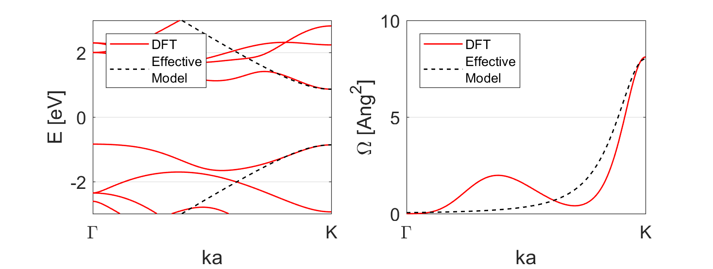
Imaging the valley Hall effect in insulating TMD – As an application of our formalism, we consider a monolayer of MoS2 in the 2H phase. We’ll show the relation between the electric field-induced change in density and the valley Hall effect for three cases of increasing complexity: the response at a single point, the net response in the insulating phase, and the energy-resolved response. MoS2 is a nonmagnetic direct band-gap semiconductor Mak et al. 2010, and its crystal and electronic structure are shown Fig. 1(a) and (b), respectively. It has a direct band gap of (computed value) located at , where is the in-plane lattice constant. (Note that is often labeled .) Figs. 1 (c) and (d) show the -dependent Berry curvature and orbital Hall conductivity, respectively. For energies away from the band edge, the valley index of a state can be associated with the nearest valley, but the label becomes less well-defined.
The unit cell contains 2 S atoms and 1 Mo atom, and there is significant - orbital hybridization in some regions of the band structure. The states near the band gap at and exhibit the largest contribution to the Berry curvature. These states are composed primarily of -orbitals localized on the Mo atoms, which form a hexagonal lattice, and which do approximately satisfy the assumptions of our analysis. The conduction band is composed of states, corresponding to , while the valence band is states at , corresponding to Xiao et al. 2012. These essential features are shared by other 2H TMD’s Xiao et al. 2012, so that our formalism is applicable to this family of materials.

In the vicinity of , the conduction and valence bands are described by a massive Dirac Hamiltonian Xiao et al. 2012. Letting , we have:
| (7) |
where is the Pauli matrix in the space of conduction and valence band states, and is the valley index. We ignore the spin degree of freedom, as it doesn’t play an essential role and makes quantitative contributions on the order of , where is the atomic spin-orbit parameter Bhowal and Satpathy 2020. In MoS2 this ratio is approximately . For TMD’s composed of heavier elements, the larger spin-orbit splitting will change some details of the analysis that we present here.
We first consider the currents and charge densities of the equilibrium states at (or ). The eigenstates are and . The factor of Eq. 4 contributes to the bond currents as indicated by the bond-aligned arrows Fig. 2(a). The charge density of both conduction and valence band equilibrium states is isotropic in the - plane, so that the bond currents are weighted equally and the net current vanishes.

Applying an electric field in the -direction perturbs the valence band wave function: , where is the magnitude of the electric charge. The mixing of valence and conduction band states leads to an anisotropic which overlaps unevenly with the nearest neighbor bonds. This in turn breaks the balance of bond currents between nearest neighbors and enables a nonzero net current, corresponding to the transverse conductivity or Berry curvature . The modification of the density for electric fields along and -directions is depicted schematically in Fig. 2(b) and (c), and provides an intuitive rationale for the formation of Hall current at the point Mak et al. 2014; Lee et al. 2016.

To test the quantitative validity of Eq. 4 for MoS2, we compute the electric field-induced change in charge density of the conduction band state at using the first principles tight-binding Hamiltonian and real space orbitals obtained with Quantum Espresso et al 2017 and Wannier90 Mostofi et al. 2014. We can independently compute both left and right-hand sides of Eq. 6 in a model with no approximations beyond those found in density functional theory. This provides a stringent test on the applicability of our formalism to real materials, and yields a prediction for the observable quantity . Fig. 3(a) shows isosurface contours of the electric field-induced change in density for the conduction band state at , for an applied electric field along the -direction. Fig. 3(b) shows in the plane of the Mo atoms, and Fig. 3(c) shows the density along a line connecting nearest neighbors. From the profile, we extract the (normalized) radial part to obtain . Applying Eq. 4 leads to
| (8) |
We use a value of obtained by fitting the conduction/valence bands to the effective model near . Plugging in numbers we obtain a predicted value from the real space density analysis, compared to the directly computed value . We find semi-quantitative agreement between the two values, validating the applicability of our approach to real materials. The difference between the two quantities is traced back to the nonzero contribution of the orbitals of the wave function at .
We next extend our analysis to the full, -integrated response for the insulating system. The Berry curvature at finite is given by:
| (9) |
The valley Hall conductivity of the effective model is obtained by integrating over and summing over , which results in . (We omit factors of in reporting conductivity values.) The values for and obtained with first principles calculations, which are given by and , respectively. The deviations between conductivities obtain with the effective model and first principles reflect the difference between the two models’ band structure. In the Supp. Info, we show that the -dependent perturbed density is proportional to the Berry curvature:
| (10) |
where is the -like atomic wave function for the conduction (valence) band state. Importantly, the change in charge density and the Berry curvature have the same -dependence. Integrating Eq. 10 over relates the total change in charge density to the valley Hall conductivity. Fig. 3(d) shows the line cut of the total change in charge density along . We can derive the following relation between the extrema of the change in charge density along and valley Hall conductivity:
| (11) |
where . Using the change in density obtained from first principles and Eq. 11, we obtain an estimated value for of . This compares well with the directly computed value of valley Hall conductivity. The comparison with the orbital Hall conductivity is more favorable, which is a consequence of the close relationship between the valley and orbital Hall conductivity in this material, and because the orbital Hall conductivity is more strongly concentrated near the points (see Fig. 1(d)). The good agreement between the directly computed and the value predicted with our real space analysis again demonstrates the applicability of our approach to real materials.
Valley/orbital Hall spectroscopy – We next consider the energy-resolved valley/orbital Hall conductivities and change in density. We again focus on a linecut along the -direction, and assume that the measured local density of states is proportional the integral of the density along the direction (e.g., the integral of Eq. 10 along ). In the Supp. info we show that:
| (12) |
where is the position of the minimum in the change of density (see Fig. 4(a)). The proportionality between the -dependent change in charge density and the Berry curvature implies that the two quantities are also proportional when integrating over . In particular, the energy-resolved quantities are proportional. Denoting the energy-resolved density, or local density of states, as , we find:
| (13) |

Fig. 4(a) shows the energy-resolved change in density for three energies below the valence band edge. Fig. 4(b) shows a comparison between the directly computed valley Hall/orbital conductivity and the predicted value based on Eq. 13. We see semi-quantitative agreement up to 500 meV away from conduction and valence band edges. We observe that the change in density adheres more closely to the orbital Hall effect at energies away from the band edges. This is due to the fact that the change in density and orbital Hall effect are dominated by states near for most energies, whereas the valley Hall conductivity acquires contributions from states near () at energies away from the band edges.
To summarize, we show that the real space density response of TMD’s such as MoS2 provides a direct estimate of the intrinsic valley Hall conductivity. This is a consequence of a relation we derive between the Berry curvature and the charge density response of a specific class of lattices. Experimentally, various probes attain the required sub-Angstrom spatial resolution, such as X-ray diffraction Wahlberg et al. 2015, electron beam diffraction Gao et al. 2019, and scanning tunneling microscopy Jelínek 2017. We estimate a fractional change of the local density of states on the order of at the breakdown electric field of MoS2 Lembke and Kis 2012. The measurement can be calibrated with the ground state density or LDOS, as described in the Supp. Info, enabling the quantitative estimate of the valley Hall conductivity.
F.X. acknowledges support under the Cooperative Research Agreement between the University of Maryland and the National Institute of Standards and Technology Physical Measurement Laboratory, Award 70NANB14H209, through the University of Maryland.
References
- Xiao et al. (2012) D. Xiao, G.-B. Liu, W. Feng, X. Xu, and W. Yao, Physical review letters 108, 196802 (2012).
- Xiao et al. (2010) D. Xiao, M.-C. Chang, and Q. Niu, Rev. Mod. Phys. 82, 1959 (2010).
- Lee et al. (2016) J. Lee, K. F. Mak, and J. Shan, Nature nanotechnology 11, 421 (2016).
- Srivastava et al. (2015) A. Srivastava, M. Sidler, A. V. Allain, D. S. Lembke, A. Kis, and A. Imamoğlu, Nature Physics 11, 141 (2015).
- Ubrig et al. (2017) N. Ubrig, S. Jo, M. Philippi, D. Costanzo, H. Berger, A. B. Kuzmenko, and A. F. Morpurgo, Nano letters 17, 5719 (2017).
- Mak et al. (2012) K. F. Mak, K. He, J. Shan, and T. F. Heinz, Nature nanotechnology 7, 494 (2012).
- Mak et al. (2014) K. F. Mak, K. L. McGill, J. Park, and P. L. McEuen, Science 344, 1489 (2014).
- Hung et al. (2019) T. Y. Hung, K. Y. Camsari, S. Zhang, P. Upadhyaya, and Z. Chen, Science advances 5, eaau6478 (2019).
- Wu et al. (2019) Z. Wu, B. T. Zhou, X. Cai, P. Cheung, G.-B. Liu, M. Huang, J. Lin, T. Han, L. An, Y. Wang, et al., Nature communications 10, 1 (2019).
- Harrison (2012) W. A. Harrison, Electronic structure and the properties of solids: the physics of the chemical bond (Courier Corporation, 2012).
- Slater and Koster (1954) J. C. Slater and G. F. Koster, Phys. Rev. 94, 1498 (1954).
- Nagaosa et al. (2010) N. Nagaosa, J. Sinova, S. Onoda, A. H. MacDonald, and N. P. Ong, Reviews of modern physics 82, 1539 (2010).
- Bernevig et al. (2005) B. A. Bernevig, T. L. Hughes, and S.-C. Zhang, Physical review letters 95, 066601 (2005).
- Go et al. (2018) D. Go, D. Jo, C. Kim, and H.-W. Lee, Physical Review Letters 121, 086602 (2018).
- Bhowal and Satpathy (2020) S. Bhowal and S. Satpathy, Physical Review B 101, 121112(R) (2020).
- Canonico et al. (2020) L. M. Canonico, T. P. Cysne, A. Molina-Sanchez, R. B. Muniz, and T. G. Rappoport, Physical Review B 101, 161409(R) (2020).
- Xiao et al. (2007) D. Xiao, W. Yao, and Q. Niu, Physical Review Letters 99, 236809 (2007).
- Marrazzo and Resta (2017) A. Marrazzo and R. Resta, Physical Review B 95, 121114(R) (2017).
- Bianco and Resta (2011) R. Bianco and R. Resta, Physical Review B 84, 241106(R) (2011).
- Caio et al. (2019) M. D. Caio, G. Möller, N. R. Cooper, and M. Bhaseen, Nature Physics 15, 257 (2019).
- Mak et al. (2010) K. F. Mak, C. Lee, J. Hone, J. Shan, and T. F. Heinz, Phys. Rev. Lett. 105, 136805 (2010).
- et al (2017) P. G. et al, Journal of Physics: Condensed Matter 29, 465901 (2017).
- Mostofi et al. (2014) A. A. Mostofi, J. R. Yates, G. Pizzi, Y.-S. Lee, I. Souza, D. Vanderbilt, and N. Marzari, Computer Physics Communications 185, 2309 (2014).
- Wahlberg et al. (2015) N. Wahlberg, N. Bindzus, L. Bjerg, J. Becker, S. Christensen, A.-C. Dippel, M. R. Jørgensen, and B. B. Iversen, The Journal of Physical Chemistry C 119, 6164 (2015).
- Gao et al. (2019) W. Gao, C. Addiego, H. Wang, X. Yan, Y. Hou, D. Ji, C. Heikes, Y. Zhang, L. Li, H. Huyan, et al., Nature 575, 480 (2019).
- Jelínek (2017) P. Jelínek, Journal of Physics: Condensed Matter 29, 343002 (2017).
- Lembke and Kis (2012) D. Lembke and A. Kis, ACS nano 6, 10070 (2012).
Supplementary Information for “Imaging the valley and orbital Hall effect in monolayer MoS2”
I Relation Between density and current
In this section we derive the derivation of the relation between a state’s charge density distribution and its velocity in a tight-binding model. This relation holds only for a lattice composed of a monoatomic unit cell, with orbitals of the same character (e.g., or orbitals), and a crystal field Hamiltonian with only -hopping. This analysis is therefore qualitatively valid for cases in which are sufficiently less than bonding. This is often the case, and in the next section we provide an explicit description of the validity of this assumption.
The tight-binding model is represented in real-valued spherical harmonics. We denote these by , which are linear combinations of and . Letting :
| (14) |
The specific forms of the real spherical harmonics for a given can be found in various references. Generally the label is expressed in terms of the cartesian factors corresponding to the form of the spherical harmonic (e.g. for is labeled as ).
In the tight-binding formulation, the -bonding hopping parameter is defined as the hopping between orbitals displaced along the -direction.
| (15) |
The hopping between orbital and displaced along the direction is then determined by projecting each orbital along the (see Fig. 5(a) and (b)). This projection is obtained by rotating the into the -direction (see Fig. 5) We review this procedure next.
We denote the axis of quantization for the spherical harmonic in the subscript of the ket: . The operator which rotates into is denoted by :
| (16) |
The rotated spherical harmonic can be written as a linear combination of unrotated spherical harmonics with the same value of , written in terms of the Wigner -matrix:
| (17) |
Crucially, for the elements of are equal to the value of the spherical harmonic evaluated at .
| (18) |
The projection of onto orbital is then given by Eq. 18. As described in the previous paragraph, this quantity provides the angular dependence of the hopping between orbitals displaced by .
| (19) |

The -hopping contribution between orbital and displaced by is therefore equal to and :
| (20) |
The denominator of Eq. 20 is a normalization factor that ensures that Eq. 15 is recovered for hopping between orbitals displaced along the -direction (i.e., for ).
This form of leads to the relation between current and density. We write the general form of the current:
| (21) |
Next we write the equation for the density from primary unit cell orbitals:
| (22) | |||||
| (23) |
As described in the main text, the charge density is the product of a radial function and an angular function
| (24) |
where and
| (25) |
Combining Eqs. 20, 21, and 25, we obtain:
| (26) |
is the -dependent value of the sigma-bonding hopping integral, whose generally parameterized form can be found in the following section.
II Limit of validity for -hopping tight-binding
The previous derivation applies for -hopping. Generally and -hopping can be quantitatively, and even qualitatively as important as -hopping. The relative importance of different hopping terms depends on the type of inter-orbital hopping and the relative orientation of the two orbitals. Fig. 7 shows both the -hopping and total hopping amplitudes for all of the unique interorbital hopping for , as a function of relative orientation (parameterized by polar angles ). The form of the tight-binding matrix elements are taken from Harrison 2012. For -orbitals, the parameterization is: , and the hopping is Harrison 2012:
| (27) |
Fig. 6 shows that for -orbitals, the -hopping is always a good semi-quantitative estimate of the total hopping for all configurations.

For (-orbitals), the parameters are taken to be , and the hopping is Harrison 2012:
| (28) |
where is another parameter, and is typically element-specific. A similar conclusion of the predominance of -hopping is reached for orbitals(Fig. 7), with one notable exception: the total hopping and -hopping are off by a minus sign for most orbital configurations. However for all other orbital pairs, the -hopping at least qualitatively, and often semi-quantitatively provides a representation of the total hopping.

III Real space density calculations
We describe the procedure used to obtain the real space density associated with the perturbed eigenstates. We first obtain the real space orbitals from Wannier90, extending out 2 unit cells away from the atom center (so that the density is represented in a supercell). The wave function is expressed as a linear combination of these basis orbitals:
| (29) |
The -dependence of the wave function coefficients is given by Bloch phase factors. We form the perturbed state as:
| (30) |
where is a small parameter.
Given a set of occupied states, the associated density matrix is given by the outer product of the states:
| (31) |
The real space density associated with the density matrix is:
| (32) |
IV Relation between total density versus primary unit cell density

The density which enters into the relation between velocity and charge density is not the total density, but the density contribution from “on-site” orbitals . The operator form is as given in the main text:
| (33) |
In terms of the density matrix, this quantity is:
| (34) |
corresponds to only including terms in Eq. 32. The charge density in the interstitial regions is quite different for and . However in the vicinity of the nuclei, these densities are quite similar. We show this explicitly in Fig. 8, where we plot and for applied field in and directions in MoS2. As expected, the quantitative difference is quite small near the nuclei. This can be generally anticipated for states with high Berry curvature: Berry curvature is related to the formation of orbital moments, which requires higher values of . These states are more localized than, for example, -like states.
V Real space calculation for MoS2
We begin our analysis of MoS2 by considering the effective model near the points. We let be the Bloch momentum vector measured from the point. The effective model Hamiltonian is:
where is the valley index and is the lattice constant. The eigenvalues for both valleys are given by:
| (38) |
It’s straightforward to show that the Berry curvature is given by:
| (39) |
We next record the full form of the wave functions of conduction and valence bands (denoted by and , respectively) at , which form the Hilbert space for nonzero :
| (40) | |||||
| (41) | |||||
| (42) | |||||
| (43) |
where . is the effective Bohr radius of the orbital. The various normalization factors are:
| (44) | |||||
| (45) |
Notice that the radial wave function has a prefactor of in the numerator, while the spherical harmonic has a factor of in the denominator, the two of which cancel each other.
To determine the form of the perturbed wave functions, and resulting real space density away from the point (), we return to the effective model:
The unperturbed eigenstates are spinors oriented along the direction of the pseudo effective field .
where . Recall that the psuedospin basis functions are combinations of the -orbitals:
| (58) | |||||
| (62) | |||||
The perturbed wave function is:
| (63) |
Let’s consider .
If we evaluate the 1st order change in the wave function, we find that following expression, where we include the functional form of the angular part of the orbitals:
| (69) |
Since , we can approximate the above as:
| (70) | |||||
| (71) |
Note that the unit for is the standard unit for density, . We find an identical expression for , so that the net density is nonzero when summing over valleys.
VI Insulating case: relating and
We integrate over (or ) to find the total valley Hall conductivity in the insulating case:
| (72) | |||||
| (73) | |||||
| (74) |
The total (integrated) change in density is given by:
| (75) |
A factor of 2 in the above is the result of summing over . Note the units of , the “total” density, are , which include a factor of from the standard density unit, and an additional factor from the Brillouin zone integration.
Next we connect the two quantities by picking out a specific point . The natural point is the maximum of the density along the -direction, for . Letting :
| (76) |
In the above is the effective Bohr radius The minimum value of is located at . At this point:
| (77) |
We use Eq. 73 to rewrite the term in brackets on the right-hand-side of the above as:
| (78) |
equivalently:
| (79) |
We can test this picture by separately computing the two sides of Eq. 79, which is presented in the main text.
VII Change in local density of states
For the local density of states calculation, we focus on and will integrate the density over . Re-writing Eq. 71:
| (80) |
Here we omit the label for , as the density is equal for both values as described earlier. Generally, a two-dimensional map of charge density obtained with scanning tunneling microscopy (STM) involves a convolution over the depth . The precise form of this convolution function depends on the experimental details. For the sake of simplicity, we choose in the analysis presented here. Generalizing to other forms of is straightforward, and will result in different numerical prefactors whose precise value is important for quantitative data analysis. Proceeding with , we obtain:
| (81) |
To determine the position of the absolute value of the maximum of this function, we first make integral dimensionless with . We also include the numerical prefactors explicitly:
| (83) |
Next write in dimensionless form, .
| (84) |
The integral in Eq. 84 must be evaluated numerically for each value of . The resulting dimensionless form of the function in brackets is shown in Fig. 10.

The position of the minimum is at , and the value of the function there (in dimension-ful form) is . We combine these two facts to obtain:
| (85) |
Using the expression for in Eq. 39, we arrive at Eq. 14 of the main text:
| (86) |
VII.1 Energy-resolved Hall conductivity
We next discuss the energy-resolved Berry curvature, and the energy-resolved change in charge density distribution. We will find a simple relationship between these two quantities. The general expression for the energy-resolved valley Hall and orbital Hall conductivity are:
| (87) | |||||
| (88) |
where , , and . In Eq. 87, is according to the state’s valley index.
Using Eq. 85, we obtain:
| (89) |
VIII Calibration of the local density of states measurement
The differential conductance measured in an STM experiment is proportional to the local density of states, and the constant of proportionality may depend on experimental details and may be unknown. However, Eq. (13) of the main text relies on the absolute value of the local density of states. In order to calibrate the measurement, we provide the equilibrium local density of states at the valence band edge energy in Fig. 11. As before, we assume that the measured signal is proportional to the integral over the coordinate. The local density of states exhibits a maximum value at the center of the Mo atom, with a value of . Fig. 11(c) shows the electric field induced change in the density of states, normalized by this maximum value. By normalizing the data this way, the unknown constant of proportionality between the signal and the local density of states factors out of the data.
The unit of the normalized change in LDOS is inverse electric field, and provides the fractional change of the local density of states for a given applied electric field. To achieve a fractional change of requires an applied field of . As mentioned in the main text, this is on the order of the breakdown field measured for MoS2 Lembke and Kis 2012, so that the effect we describe is quantifiable for measurements with signal to noise ratio of less than .
