Unifying continuous, discrete, and hybrid susceptible-infected-recovered processes on networks
Abstract
Waiting times between two consecutive infection and recovery events in spreading processes are often assumed to be exponentially distributed, which results in Markovian (i.e., memoryless) continuous spreading dynamics. However, this is not taking into account memory (correlation) effects and discrete interactions that have been identified as relevant in social, transportation, and disease dynamics. We introduce a framework to model continuous, discrete, and hybrid forms of (non-)Markovian susceptible-infected-recovered (SIR) stochastic processes on networks. The hybrid SIR processes that we study in this paper describe infections as discrete-time Markovian and recovery events as continuous-time non-Markovian processes, which mimic the distribution of cell cycles. Our results suggest that the effective-infection-rate description of epidemic processes fails to uniquely capture the behavior of such hybrid and also general non-Markovian disease dynamics. Providing a unifying description of general Markovian and non-Markovian disease outbreaks, we instead show that the mean transmissibility produces the same phase diagrams independent of the underlying inter-event-time distributions.
I Introduction
Models of epidemic processes such as the susceptible-infected-recovered (SIR) model and related models provided various insights into dynamical and stationary features of disease, opinion, and failure spread in social and technical systems Pastor-Satorras et al. 2015; Böttcher et al. 2017a; Antulov-Fantulin et al. 2015. In the SIR model, infected individuals may transmit a disease to susceptible ones. After a certain period, infected individuals recover and are not part of the disease-transmission process anymore. The exact time evolution of the continuous-time stochastic SIR spreading process is described by the Chapman-Kolmogorov equation or its differential form (i.e., the master equation). However, exact analytical solutions of the master equation are limited to special cases and therefore different approximations are being used (e.g., deterministic ODE models Moreno et al. 2002; Keeling and Rohani 2011; Sharkey 2011, cavity-like models Sharkey et al. 2015; Karrer and Newman 2010, and pairwise approaches Sherborne et al. 2018).
Gillespie and kinetic Monte-Carlo (kMC) approaches Gillespie 1976 provide techniques to generate statistically exact trajectories of a master equation. The assumption underlying kMC simulations of SIR processes is that waiting times between consecutive recovery and infection events are exponentially distributed. However, many natural processes including social dynamics Barabasi 2005; Böttcher et al. 2017b exhibit correlation and memory (i.e., non-Markovian) effects Goh and Barabási 2008 and are therefore not described by exponential (i.e., memoryless) waiting-time distributions Starnini et al. 2017. Recent attempts to simulate general non-Markovian processes led to the development of the non-Markovian Gillespie algorithm (nMGA) Boguná et al. 2014 and the Laplace Gillespie algorithm (LGA) Masuda and Rocha 2018. Both methods are based on a mapping of multiple stochastic processes with general (continuous) waiting-time distributions to a modified kMC algorithm. As outlined in Ref. Masuda and Rocha 2018, the nMGA is exact only for infinitely many processes and requires to re-calculate all individual rates at every time step. This algorithm has the advantage that it can simulate arbitrary continuous inter-event-time distributions Boguná et al. 2014. The LGA interprets survival functions of waiting-time distributions as Laplace transforms of underlying event-rate distributions. Although the LGA is exact for arbitrary numbers of processes, it is only applicable to certain waiting-time distributions Masuda and Rocha 2018.
In the context of non-Markovian SIR models, there also exist event-driven and directed-percolation-based approaches that are directly applicable to these types of processes Tolić et al. 2018; Istvan et al. 2019. In this paper, we use an approach similar to the directed-percolation method of Refs. Tolić et al. 2018; Istvan et al. 2019 and map non-Markovian SIR processes with general waiting-time distributions to a shortest-path problem Kulkarni 1986; Corea and Kulkarni 1993 in a weighted spreading network. We refer to this method as shortest-path kinetic Monte Carlo (SPkMC). In contrast to the nMGA, LGA, and aforementioned approximation techniques Moreno et al. 2002; Keeling and Rohani 2011; Sharkey 2011; Sharkey et al. 2015; Karrer and Newman 2010; Sherborne et al. 2018, our SPkMC framework allows us to produce exact stochastic trajectories of SIR processes for general continuous and discrete waiting-time distributions on any network.

We use our framework to study continuous, discrete, and hybrid SIR processes. Such hybrid formulations of spreading dynamics can be useful to account for events that are generated according to a sequence of fixed-duration schedules (e.g., meeting Panko and Kinney 1995, patient care Rea et al. 2007; Duval et al. 2018, and transportation schedules Dorfman and Medanic 2004) and (ii) finite transfer times of information in communication networks Chen et al. 2003.
Various processes that affect human interaction and information exchange in communication networks can be modeled as discrete events. Possible examples include sequences of fixed-duration schedules of meetings (multiples of hours and minutes) Panko and Kinney 1995; Rea et al. 2007; Duval et al. 2018 and transportation schedules Dorfman and Medanic 2004 that can affect disease transmission on a meta-population level. For communication networks, finite transfer times and synced digital events (e.g., release of computer viruses) are also examples of discrete processes Chen et al. 2003.
In addition, hybrid SIR models can also account for latency periods that are typically modeled by introducing an additional “exposed” compartment Keeling and Rohani 2011 and a corresponding latent period, which mimics the observed mean incubation time (e.g., 8-14 days for measles Lessler et al. 2009). As an alternative to discrete Allen 1994; Zhou et al. 2004; Chen 2019 and continuous Keeling and Rohani 2011 epidemic models with “exposed” compartments, our approach can account for discrete time delays by directly modifying transmission rates.
Our results suggest that hybrid and also general non-Markovian disease outbreaks cannot be uniquely captured by effective infection rates. However, by mapping hybrid SIR processes to bond percolation Grassberger 1983; Newman 2002, we show that the corresponding mean transmissibilities produce the same phase diagrams independent of the underlying infection- and recovery-time distributions; thus providing a unifying description of general Markovian and non-Markovian SIR processes. The framework we propose assumes no specific form of waiting-time distributions Chen 2019; Fennell et al. 2016 and allows us to simulate and analytically describe general discrete, continuous, and hybrid variants of Markovian and non-Markovian SIR dynamics.
II Shortest-path kinetic Monte Carlo
Before focusing on the simulation of hybrid SIR dynamics, we introduce the necessary mathematical toolbox that allows us to map general waiting times to a shortest-path problem in an underlying spreading network. Let and be the probability-density or probability mass functions (PDFs or PMFs) of recovery and infection times. In continuous time, the probability that a recovery (infection) event occurs in the interval is (). The discrete time analogues and are the recovery and infection probabilities after steps, where denotes the floor function. We denote the cumulative distribution function (CDF) of and by and . The function () is the probability that a recovery (infection) event occurred in . In the case of Poissonian SIR dynamics, waiting-time distributions are described by the PDFs and and CDFs and , where and are the corresponding recovery and infection rates. Note that we use prefixes such as “Erlang-geometric” to indicate the recovery and infection time distributions ( and ) of the corresponding hybrid SIR process.
For given distributions and , we consider realizations of SIR dynamics to correspond to an ensemble of directed spreading networks , where and denote the sets of nodes and edges. Each network is initialized as follows. For each node in , we generate a random number and use an inverse transform sampling of to determine the recovery time of node according to . For each node that is adjacent to , we generate another random number and determine the infection time . We now use and to determine edge weights Tolić et al. 2018
| (1) |
We set to (i.e., the disease transmission time from node to ) if infection occurs before recovery, and otherwise. Note that the interaction terms can also be general , where accounts for node-dependent transmission features like age, gender, and other social and demographic factors including interventions like the probability of quarantine or contact containment restrictions. If the CDFs are not invertible, we can generate edge weights with rejection sampling. In Fig. 1 (a), we show an illustration of the weight initialization procedure for a network that consists of 4 nodes. We again note that networks are directed (i.e., weights may be different from ). In the case of Poissonian dynamics, we obtain
| (2) |
In addition to edge weights, we also keep track of node weights to describe the evolution of SIR dynamics in a network.

After having identified all weights, we obtain one realization of the spreading network. In the next step, we take and infect one uniformly at random selected node (see Fig. 1 (b)). All nodes that are connected to the initially infected node through paths of finite length are also infected and recover in the limit of (see Fig. 1 (c)). The shortest-path length between an infected source and its target node is the corresponding disease transmission time. This formulation of disease transmission can be viewed as a “least action principle” for kMC. If all paths that connect two nodes are infinite, we know that one or multiple recovered (or quarantined/removed) nodes hinder disease transmission (see node 4 in Fig. 1). To describe SIR dynamics with initially infected nodes, we use to denote the set of infected nodes that result from an initial infection of node in . The corresponding set of all infected nodes that result from multiple spreading seeds in is . The SPkMC framework also allows us to monitor the infection and recovery times of individual nodes. In App. A and App. B, we outline how the evolution of susceptible, infected, and recovered nodes can be reconstructed from shortest paths and describe the possibility to account for quarantine protocols in SPkMC simulations.
The stationary fraction of recovered nodes in network is , where is the number of nodes, and the corresponding ensemble average over yields
| (3) |
For each network realization , we have to identify all shortest paths, an operation with run time of order when using optimized data structures such as Fibonacci heaps Fredman and Tarjan 1987. For initially infected nodes, we can determine the number of susceptible , infected , and recovered nodes at time (see App. A) after running Dijkstra’s algorithm times. Typically, the number of initially infected nodes is small and thus the run time of our algorithm is still of order . Reference Masuda and Rocha 2018 discusses the run time complexity of the nMGA and LGA per generated event. Since our SPkMC framework can simulate SIR dynamics with one run of Dijkstra’s algorithm, the computational complexity of our framework does not depend on the number of time steps that one wants to simulate.
In App. C, we consider Poissonian dynamics (see Eq. (2)) and show that our SPkMC simulations of stationary and dynamical SIR features agree well with corresponding kMC simulations. An advantage of our proposed shortest-path SIR simulation method is the possibility to simulate general Markovian and non-Markovian dynamics with continuous and discrete waiting time distributions.
III Hybrid continuous-discrete SIR dynamics
To describe latency periods in infection processes (i.e., no infection occurs during a certain time window), we apply our simulation framework to hybrid Poisson-geometric SIR dynamics with discrete infection events that are distributed according to a geometric density function
| (4) |
where is the probability that an infection event occurs within a time step of 1 and is the Dirac delta function. We show in App. D that the master equation of hybrid Poisson-geometric SIR dynamics is no longer time-homogeneous. In App. E, we also consider an alternative definition of the geometric distribution that takes on finite values for all non-negative integers. The geometric distribution is the discrete memoryless counterpart of exponential distributions.
We can now use our simulation framework to study disease outbreak characteristics of such hybrid SIR processes. As for many epidemic processes Keeling and Rohani 2011, we characterize disease dynamics in terms of the effective infection rate , where and are the mean times to infection and recovery, respectively. For a fully Poissonian SIR process, the effective infection rate is and invariant upon rescaling of infection and recovery rates by a constant factor Pastor-Satorras et al. 2015. That is, the corresponding fraction of recovered (see Eq. (3)) only depends on the effective infection rate (see Fig. 2 (top)). By analogy, we now use to denote the effective infection rate for Poissonian-geometric dynamics with infection-time PDF and
| (5) |
However, unlike in fully Poissonian SIR dynamics, we cannot uniquely capture the corresponding phase space by the effective infection rate (see Fig. 2 (bottom)). That is, we observe different fractions of recovered for the same value of . To better understand the phase space of hybrid SIR processes, we proceed with a mapping to bond percolation.
IV Mapping hybrid SIR dynamics to bond percolation
We now analytically characterize the hybrid SIR disease prevalence in terms of the mean transmissibility that describes the probability of an infection to be transmitted from an infected to an adjacent susceptible node Newman 2002:
| (6) |
In networks with no degree correlations, the critical transmissibility above which an SIR epidemic spreads through a finite fraction of the system is given by the bond percolation threshold Newman 2002; Pastor-Satorras et al. 2015
| (7) |
where and denote the first and second moment of the degree distribution .
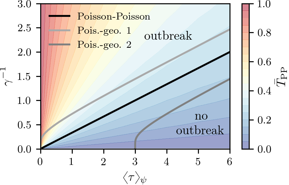
For Poisson-geometric SIR dynamics, the mean transmissibility is
| (8) | ||||
In App. E, we provide further details about the derivation of Eq. (8) and compare the fully Poissonian and Poisson-geometric case. According to Eqs. (7) and (8), we find the phase separation line , which separates the phases with and without disease outbreaks (see Fig. 3). For and , we obtain the critical effective infection rates and , respectively. These values agree well with the numerical data of Fig. 2 (bottom).
Note that cannot be parametrized in terms of an effective infection rate (see Fig. 3) whereas for fully Poissonian dynamics the mean transmissibility only depends on the effective infection rate (see App. C and Ref. Newman 2002). However, if is small, we find that
| (9) |
Thus, for sufficiently small values of and (i.e., long mean infection and recovery times), the mean transmissibility only depends on the effective infection rate . In the SI, we show that this is also the case for the alternative formulation of Poisson-geometric SIR dynamics with . A graphical interpretation of this result is that the phase separation lines in Fig. 3 merge as and tend to infinity.
To determine the relative size of the epidemic as function of the mean transmissibility , we use a generating-function approach Newman 2002 and first consider an uncorrelated network for which the conditional probability does not depend on . This approach is based on two generating functions and . The former is the generating function of the distribution of occupied edges belonging to a certain node, as a function of Newman 2002:
| (10) |
The distribution of occupied edges leaving a node at which we arrived by following a randomly selected edge is generated by Newman 2002
| (11) |
Note that we use to indicate a derivative of with respect to . To determine (see Eq. (13)), we solve the self-consistency equation
| (12) |
and compute
| (13) |
where is the probability that the node at the end of a randomly selected edge does not lead to a giant macroscopic component. In App. F, we generalize Eqs. (11) and (13) to account for correlation effects between nearest neighbors. Note that the generating function formalism is useful for cases when the exact network is unknown but only its degree distribution.
For details on limitations of the described bond-percolation mapping, see App. H and Refs. Kenah and Robins 2007; Trapman 2007; Karrer and Newman 2010.
As in Fig. 2, we now consider a random-regular graph with degree . The degree distribution is , where the Kronecker delta is if and zero otherwise. In Fig. 2, we show the analytical solution of Eqs. (13) and (11) for fully Poissonian () and Poisson-geometric () SIR dynamics. For a small number of initially infected nodes, the relative outbreak size corresponds to the fraction of recovered nodes (see Eq. (3)). We observe that the bond-percolation description of hybrid and fully geometric SIR (see top left panel of Fig. 4) outbreaks agree well with simulations.
V Unifying non-Markovian SIR processes

Up to this point, we focused on hybrid SIR processes with variations in the infection-time distributions. To understand the general applicability of our framework, we now consider non-Markovian SIR dynamics with recovery times that are distributed according to the Erlang distribution
| (14) |
where and are the so-called shape and rate parameters. The Erlang distribution allows us to account for recovery processes that are not just exponentially distributed but more concentrated within a certain time window. It is the distribution that describes the sum of independent exponential variables with rate . The Erlang distribution has been used as an approximation of cell-cycle time distributions Yates et al. 2017 and as such it is a good candidate for disease recovery processes as cells cycles have stages through which they are progressing (e.g., for COVID-19 Pan et al. 2020). In Fig. 4 (top right), we observe that Erlang-geometric SIR processes can also not be described by an effective infection rate. The considered examples of non-Markovian SIR processes show that the effective-spreading-rate description cannot uniquely characterize hybrid and general non-Markovian disease outbreaks. Instead, the mean transmissibility provides a unifying control parameter as we show in Fig. 4 (bottom). In App. G, we outline that this also holds for other networks including Erdős-Rényi, Barabási-Albert, and various empirical networks.
VI Discussion and conclusion
We introduced numerical and analytical frameworks for the study of general (non-)Markovian SIR dynamics on networks. Furthermore, we proposed a novel hybrid SIR process that models infection and recovery as discrete-time Markovian and continuous-time (non-)Markovian processes, respectively. The discussed examples of hybrid SIR processes can account for cell-cycle distributions and latency intervals during which no infection events occur. We showed that the effective-infection-rate description of Markovian SIR processes Pastor-Satorras et al. 2015 cannot uniquely capture non-Markovian epidemic outbreaks. However, our results suggest that the mean transmissibility provides a unifying description of (non-)Markovian SIR processes across a wide range of network structures (see App. G) and infection and recovery time distributions. These observations are of particular interest for disease control and hint at a re-definition of the epidemic threshold to appropriately account for disease dynamics and network structure Liu et al. 2018. Our results also complement an earlier study on non-Markovian SIR dynamics Min et al. 2013, which showed that strong temporal heterogeneity in the contact patterns between individuals may significantly suppress epidemic outbreaks.
Further motivation for the study of discrete interaction processes comes from temporal-network theory, where the majority of temporal interactions is considered to be discrete Clauset and Eagle 2012; Holme 2015. Future studies may extend our work to hybrid models on temporal networks.
Our findings are in accordance with earlier results on non-Markovian susceptible-infected-susceptible (SIS) dynamics Starnini et al. 2017, where a modified effective infection rate was used to uniquely capture corresponding steady states. A mean-field analysis of SIS dynamics Feng et al. 2019 also revealed that there is an equivalence between certain non-Markovian and Markovian SIS processes. Similar concepts may be helpful to better understand similarities between non-Markovian and Markovian SIR dynamics.
To summarize, our work can contribute to more accurate and informative models of spreading processes on networks and meta-population spreading models Colizza and Vespignani 2008; Van den Broeck et al. 2011.
Acknowledgements.
We thank Jan Nagler for helpful comments. LB acknowledges financial support from the SNF Early Postdoc.Mobility fellowship on “Multispecies interacting stochastic systems in biology” and the Army Research Office (W911NF-18-1-0345). N.A-F. acknowledges financial support from ’SoBigData++’ with grant agreement 871042. L.B. and N.A-F. contributed equally to this work.References
- Pastor-Satorras et al. (2015) R. Pastor-Satorras, C. Castellano, P. Van Mieghem, and A. Vespignani, Rev. Mod. Phys. 87, 925 (2015).
- Böttcher et al. (2017a) L. Böttcher, J. Nagler, and H. J. Herrmann, Phys. Rev. Lett. 118, 088301 (2017a).
- Antulov-Fantulin et al. (2015) N. Antulov-Fantulin, A. Lančić, T. Šmuc, H. Štefančić, and M. Šikić, Phys. Rev. Lett. 114, 248701 (2015).
- Moreno et al. (2002) Y. Moreno, R. Pastor-Satorras, and A. Vespignani, EPJ B 26, 521 (2002).
- Keeling and Rohani (2011) M. J. Keeling and P. Rohani, Modeling infectious diseases in humans and animals (Princeton University Press, 2011).
- Sharkey (2011) K. J. Sharkey, Theor. Pop. Biol. 79, 115 (2011).
- Sharkey et al. (2015) K. J. Sharkey, I. Z. Kiss, R. R. Wilkinson, and P. L. Simon, Bull. Math. Biol. 77, 614 (2015).
- Karrer and Newman (2010) B. Karrer and M. E. Newman, Phys. Rev. E 82, 016101 (2010).
- Sherborne et al. (2018) N. Sherborne, J. C. Miller, K. B. Blyuss, and I. Z. Kiss, J. Math. Bio. 76, 755 (2018).
- Gillespie (1976) D. T. Gillespie, J. Comp. Phys. 22, 403 (1976).
- Barabasi (2005) A.-L. Barabasi, Nature 435, 207 (2005).
- Böttcher et al. (2017b) L. Böttcher, O. Woolley-Meza, and D. Brockmann, PloS one 12, e0178062 (2017b).
- Goh and Barabási (2008) K.-I. Goh and A.-L. Barabási, EPL 81, 48002 (2008).
- Starnini et al. (2017) M. Starnini, J. P. Gleeson, and M. Boguñá, Phys. Rev. Lett. 118, 128301 (2017).
- Boguná et al. (2014) M. Boguná, L. F. Lafuerza, R. Toral, and M. Á. Serrano, Phys. Rev. E 90, 042108 (2014).
- Masuda and Rocha (2018) N. Masuda and L. E. Rocha, SIAM Review 60, 95 (2018).
- Tolić et al. (2018) D. Tolić, K.-K. Kleineberg, and N. Antulov-Fantulin, Sci. Rep. 8, 6562 (2018).
- Istvan et al. (2019) Z. Istvan, K. Miller, C. S. Joel, and L. Peter, Mathematics of Epidemics on Networks: From Exact to Approximate Models (Springer, 2019).
- Kulkarni (1986) V. G. Kulkarni, Networks 16, 255 (1986).
- Corea and Kulkarni (1993) G. A. Corea and V. G. Kulkarni, Networks 23, 175 (1993).
- Panko and Kinney (1995) R. R. Panko and S. T. Kinney, in Proceedings of the Twenty-Eighth Annual Hawaii International Conference on System Sciences, Vol. 4 (IEEE, 1995) pp. 1002–1011.
- Rea et al. (2007) E. Rea, J. Lafleche, S. Stalker, B. Guarda, H. Shapiro, I. Johnson, S. Bondy, R. Upshur, M. Russell, and M. Eliasziw, Epidemiology & Infection 135, 914 (2007).
- Duval et al. (2018) A. Duval, T. Obadia, L. Martinet, P.-Y. Boëlle, E. Fleury, D. Guillemot, L. Opatowski, and L. Temime, Scientific reports 8, 1 (2018).
- Dorfman and Medanic (2004) M. Dorfman and J. Medanic, Transportation Research Part B: Methodological 38, 81 (2004).
- Chen et al. (2003) Z. Chen, L. Gao, and K. Kwiat, in IEEE INFOCOM 2003. Twenty-second Annual Joint Conference of the IEEE Computer and Communications Societies (IEEE Cat. No. 03CH37428), Vol. 3 (IEEE, 2003) pp. 1890–1900.
- Lessler et al. (2009) J. Lessler, N. G. Reich, R. Brookmeyer, T. M. Perl, K. E. Nelson, and D. A. Cummings, Lancet Infect. Dis. 9, 291 (2009).
- Allen (1994) L. J. Allen, Math. Biosc. 124, 83 (1994).
- Zhou et al. (2004) Y. Zhou, Z. Ma, and F. Brauer, Mathematical and Computer Modelling 40, 1491 (2004).
- Chen (2019) Z. Chen, IEEE Access 7, 127669 (2019).
- Grassberger (1983) P. Grassberger, Math. Biosc. 63, 157 (1983).
- Newman (2002) M. E. Newman, Phys. Rev. E 66, 016128 (2002).
- Fennell et al. (2016) P. G. Fennell, S. Melnik, and J. P. Gleeson, Phys. Rev. E 94, 052125 (2016).
- Fredman and Tarjan (1987) M. L. Fredman and R. E. Tarjan, JACM 34, 596 (1987).
- Kenah and Robins (2007) E. Kenah and J. M. Robins, Phys. Rev. E 76, 036113 (2007).
- Trapman (2007) P. Trapman, Theor. Pop. Biol. 71, 160 (2007).
- Yates et al. (2017) C. A. Yates, M. J. Ford, and R. L. Mort, Bull. Math. Biol. 79, 2905 (2017).
- Pan et al. (2020) F. Pan, T. Ye, P. Sun, S. Gui, B. Liang, L. Li, D. Zheng, J. Wang, R. L. Hesketh, L. Yang, and C. Zheng, Radiology (2020), pMID: 32053470.
- Liu et al. (2018) Q.-H. Liu, M. Ajelli, A. Aleta, S. Merler, Y. Moreno, and A. Vespignani, Proc. Nat. Acad. Sci. USA 115, 12680 (2018).
- Min et al. (2013) B. Min, K.-I. Goh, and I.-M. Kim, EPL 103, 50002 (2013).
- Clauset and Eagle (2012) A. Clauset and N. Eagle, arXiv:1211.7343 (2012).
- Holme (2015) P. Holme, The European Physical Journal B 88, 234 (2015).
- Feng et al. (2019) M. Feng, S.-M. Cai, M. Tang, and Y.-C. Lai, Nature communications 10, 1 (2019).
- Colizza and Vespignani (2008) V. Colizza and A. Vespignani, J. Theor. Biol. 251, 450 (2008).
- Van den Broeck et al. (2011) W. Van den Broeck, C. Gioannini, B. Gonçalves, M. Quaggiotto, V. Colizza, and A. Vespignani, BMC Inf. Dis. 11, 37 (2011).
- Dijkstra et al. (1959) E. W. Dijkstra et al., Numerische mathematik 1, 269 (1959).
- Goltsev et al. (2008) A. V. Goltsev, S. N. Dorogovtsev, and J. Mendes, Phys. Rev. E 78, 051105 (2008).
- Cimini et al. (2019) G. Cimini, T. Squartini, F. Saracco, D. Garlaschelli, A. Gabrielli, and G. Caldarelli, Nature Reviews Physics 1, 58 (2019).
- Leskovec and Mcauley (2012) J. Leskovec and J. J. Mcauley, in Adv. Neur. Inf. Proc. Syst. (2012) pp. 539–547.
- (49) H. friendships network dataset KONECT, “April 2017,” .
- Mislove et al. (2007) A. Mislove, M. Marcon, K. P. Gummadi, P. Druschel, and B. Bhattacharjee, in Proceedings of the 7th ACM SIGCOMM conference on Internet measurement (2007) pp. 29–42.
- Gillespie (1977) D. T. Gillespie, J. Phys. Chem. 81, 2340 (1977).
Appendix A Dynamics reconstruction
Based on the SPkMC framework that we outline in Sec. II, we can also determine the evolution of susceptible, infected, and recovered nodes. We use to denote the mean number of non-susceptible nodes prior to some time and compute this quantity from the set of edge-weighted spreading graphs according to
| (15) |
where is the set of initially infected nodes and is the shortest-path length from node to node in the weighted spreading network . To determine the fraction of infected and recovered nodes at time , we compute the cardinality of the set of all nodes that are connected with an infected source node through a path of maximum length . To extract the dynamical behavior of infected nodes from an SPkMC simulation, we need to include node-recovery weights in our simulation framework. Similarly to Eq. (15), we determine the mean number of infected nodes according to
| (16) |
Appendix B Quarantine dynamics
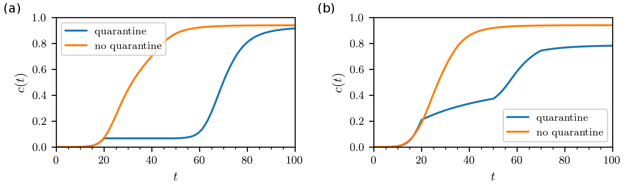
In this section, we describe the possibility to apply the SPkMC framework of Sec. II to quarantine modeling. Recall that Dijkstra’s algorithm Dijkstra et al. 1959 is constructing shortest paths via dynamic programming updates. At iteration , all distances are set to infinity, except for the source node . At iteration , we update the shortest path with the following equation:
| (17) |
where is the edge weight between nodes and .
One possible quarantine strategy would be that a pre-defined set of nodes gets removed from the network at quarantine time and brought back at time . This procedure can be repeated as often as necessary and directly incorporated in our simulation framework. Nodes can only infect others or be infected by surrounding nodes if they are not under quarantine (i.e., not removed). The outlined quarantine protocol can be implemented as follows. For a given source node , some target node , and a node that is under quarantine during , the shortest-path calculation can be extended by adapting distance updates in Dijkstra’s algorithm:
| (18) |
where is the inter-event edge transmission delay between nodes, , and is the characteristic function of :
| (19) |
According to Eq. (21), we obtain a finite shortest-path length if no quarantined node lies between nodes and . That is, is finite if for at least one node . We show an SPkMC simulation for quarantine on a random network in Fig. 5. We observe a drop in the number cumulative proportion of infections as soon as quarantine begins.
The prior quarantine protocol can be generalized as follows. Each node can have its own quarantine from time until . Accordingly, we can define and , the characteristic function of :
| (20) |
Now, for a given source node , some target node , and a node that lies on the path between and , the shortest-path calculation in Dijkstra’s algorithm can be extended by adapting the dynamic programming update:
| (21) |
where the characteristic function of node prohibits transmission from node if it is under quarantine and the characteristic function prohibits transmission to node if it is under quarantine.
Appendix C Comparison of algorithms

Here, we compare the stationary and transient behavior of fully Poissonian SIR dynamics that we obtain with SPkMC and kMC simulations Istvan et al. 2019 (see Fig. 6). We consider a regular random network with degree and nodes. For Poissonian infection and recovery times, the mean transmissibility is Newman 2002
| (22) |
where the effective infection rate is . This yields the threshold
| (23) |
above which giant (outbreak) components are observable. We show a comparison of the transient behavior of SPkMC and kMC simulations in Fig. 7.

Appendix D Master equation for hybrid Poisson-geometric SIR dynamics
In this section, we formulate the master equation for hybrid Poisson-geometric SIR dynamics. Let us denote the probability of finding a system in configuration at time as . The probabilities fulfill the normalization condition and the probabilistic evolution of the system is governed by the master equation:
| (24) |
The first term on the right-hand side of Eq. (24) describes the “inflow” into configuration from other configurations with transition rate and the second term accounts for the corresponding “outflow” with transition rate . In the case of SIR dynamics, every configuration is a -dimensional vector that describes the state of every node with . For hybrid Poisson-geometric SIR process, the transition rates are not constant in time anymore. This implies that the stochastic process is still Markovian, but not time-homogeneous as some transitions may only occur for integer times . We factorize the transition rates in the following way:
| (25) |
where is the adjacency matrix, denotes the local transition rate of state conditioned on the neighboring states at time . The recovery rates are constant in time:
| (26) |
However, disease transmissions only occur when the time is an integer:
| (27) |
where denotes the indicator function of the positive natural numbers , which is equal to 1 when belongs to and zero otherwise.
Appendix E Influence of discrete infection times on transmissibility
In Sec. III, we consider the following definition of the geometric distribution:
| (28) |
where is the probability that an infection event occurs within a time interval of length 1 and is the Dirac delta function. This yields the mean transmissibility
| (29) | ||||
where is the exponential recovery time distribution with recovery rate . For small , the mean transmissibility is
| (30) |
where . Based on the definition of the counting process in the Bernoulli trials, one can also define the geometric distribution where the counting starts at 1. There is no correct way, it depends on the actual definition of the stochastic process and alignment of the discrete and continuous inter-event times. Different definitions have different interpretations. For example, the above definition assumes that we allow the transmission to happen with probability at any non-negative integer number. However, if the counting process is defined over natural numbers (positive integers), it would represent the process with density
| (31) |
and mean transmissibility
| (32) | ||||

Note that the limiting behavior is in sharp contrast to the Poissonian case, where . We find for small values of and :
| (33) |
where . We show a comparison of the phase diagrams of hybrid SIR processes with infection-time distribution and in Fig. 8.
Appendix F Correlated Networks
The bond-percolation mapping that we outlined in Sec. IV is applicable to networks with an uncorrelated degree distribution (i.e., ). For networks with degree correlations, we use the notation Goltsev et al. 2008 and extend the generating-function approach of Sec. IV according to
| (34) |
where , , , and
| (35) |
This extension accounts for correlations between neighboring nodes and is based on the assumption that the considered network is locally treelike Goltsev et al. 2008. We use to denote the largest degree in the network. The function is the generating function of the distribution of occupied edges belonging to a certain node. The distribution of occupied edges leaving a node at which we arrived by following a randomly selected edge is generated by and is the probability that a node with degree at the end of an randomly selected edge is occupied. Furthermore, note that degree-degree correlations become irrelevant for the percolation transition if the spectrum of the branching matrix satisfies certain conditions Goltsev et al. 2008.
For a given network structure, we can use the SPkMC framework (see Sec. II) to simulate general (non-)Markovian SIR dynamics on a corresponding network. The generating-function approach provides a possibility to gain insights into (non-)Markovian disease outbreaks if we only know about the degree distribution of a certain network. In this case, the underlying network structure would be implicitly described by a configuration model, which corresponds to a network reconstruction using the max entropy principle Cimini et al. 2019 with a certain degree distribution as constraint. We summarize these points in Fig. 9.

Appendix G Different networks

In the main text, we outlined that effective infection rates cannot uniquely capture hybrid and general non-Markovian disease outbreaks. However, our results for random-regular networks (see Fig. 4) suggest that the mean transmissibility (see Eq. (6)) produces phase diagrams that are independent of underlying infection- and recovery-time distributions. In Fig. 10, we show that this observation can also be made for other synthetic and real-world networks. For Erdős-Rényi networks, we can use the bond-percolation description of disease outbreaks to analytically describe the phase diagram. In the case of Barabási-Albert networks, we use the generating function approach for correlated networks (see App. F) to obtain the corresponding analytical description.
Appendix H Further corrections to the percolation mapping
We utilized the SPkMC framework and Gillespie methods Gillespie 1976; Gillespie 1977 to generate exact realizations of hybrid and non-Markovian SIR dynamics and compared them to corresponding analytical (bond percolation) predictions on synthetic and real-world networks. The discussed mapping to bond percolation can be further enhanced by introducing certain corrections, which is going to be part of our future work. For example, corrections to the mean transmissibility may result from considering the probability that out of edges get activated Tolić et al. 2018:
| (36) | ||||
Note that the mean transmissibility of the main manuscript is a special case of for . In addition, corrections accounting for semi-directed spreading involve tracking down the exact direction of activated links Kenah and Robins 2007 using an extended generating function formalism.