Structure-Preserving Reduced Order Modeling of Non-Traditional Shallow Water Equation
Abstract
An energy preserving reduced order model is developed for the non-traditional shallow water equation (NTSWE) with full Coriolis force.
The NTSWE in the noncanonical Hamiltonian/Poisson form is discretized in space by finite differences. The resulting system of
ordinary differential equations is integrated in time by the energy preserving average vector field (AVF) method. The Poisson structure of the discretized NTSWE exhibits a skew-symmetric matrix depending on the state variables. An energy preserving, computationally efficient reduced order model
(ROM) is constructed by proper orthogonal decomposition with Galerkin projection. The nonlinearities are computed for the ROM efficiently by discrete empirical interpolation method. Preservation of the discrete energy and the discrete enstrophy are shown for the full order model,
and for the ROM which ensures the long term stability of the solutions. The accuracy and computational
efficiency of the ROMs are shown by two numerical test problems.
Keywords: Shallow water equation, model order reduction, Hamiltonian mechanics, finite difference methods, implicit time integrator.
1 Introduction
The shallow water equation (SWE) consists of a set of two-dimensional partial differential equations (PDEs) describing a thin inviscid fluid layer flowing over the topography in a rotating frame. SWE is a hyperbolic PDEs describing geophysical wave phenomena, e.g., the Kelvin and Rossby waves in the atmosphere and the oceans. SWEs are frequently used in large-scale geophysical flow prediction [5, 14], investigation of baroclinic instability [8, 38], and planetary flows [39]. Energy and enstrophy are the most important conserved quantities of the SWEs, whereas the energy cascades to large scales whilst enstrophy cascades to small scales [4, 37].
Real-time simulation of SWEs requires a large amount of computer memory and computing time. The reduced order models (ROMs) have emerged as a powerful approach to reduce the computational cost of evaluating large systems of PDEs like the SWE by constructing a low-dimensional linear reduced subspace, that approximately represents the solution to the system of PDEs with a significantly reduced computational cost. The solutions of the high fidelity full order model (FOM), generated by space-time discretization of PDEs are projected usually on low dimensional reduced spaces using the proper orthogonal decomposition (POD), which is the widely used reduced order modeling technique. Applying POD Galerkin projection, the dominant POD modes of the PDEs are extracted from the snapshots of the FOM solutions. The computation of the FOM solutions is performed in the offline stage, whereas the reduced system from the low-dimensional subspace is solved in the online stage. The primary challenge in producing the low dimensional models of the high dimensional discretized PDEs is the efficient evaluation of the nonlinearities. The computational cost is reduced by sampling the nonlinear terms and interpolating, known as hyper-reduction techniques [2, 3, 9, 12, 30, 41].
The naive application of POD or DEIM may not preserve the geometric structures, like the symplecticness, energy preservation and passivity of Hamiltonian, Lagrangian and port Hamiltonian PDEs. The stability of reduced models over long-time integration and the structure-preserving properties has been recently investigated in the context of Lagrangian systems [10, 23], and for port-Hamiltonian systems [11]. For linear and nonlinear Hamiltonian systems, the symplectic model reduction technique, proper symplectic decomposition (PSD) is constructed for Hamiltonian systems like linear wave equation, sine-Gordon equation, nonlinear Schrödinger equation to ensure long term stability of the reduced model [1, 32]. Recently the average vector field (AVF) method is used as a time integrator to construct reduced order models for Hamiltonian systems like Korteweg-de Vries equation [21, 29] and nonlinear Schrödinger equation [22]. Reduced order models for the SWEs are constructed in conservative form using POD-DEIM [25, 26], in the -plane by POD-DEIM and tensorial POD [15, 16], by dynamic mode decomposition [6, 7], the -plane using POD [19]. In these articles, the preservation of the energy and other conservative quantities in the reduced space are not discussed.
In this paper, we have constructed structure-preserving ROMs for the non-traditional shallow water equation (NTSWE) [17, 35, 37] with the full Coriolis force. Replacing the first order derivatives that appear in the NSTWE, a skew-gradient system, i.e. a non-canonical Hamiltonian system of ordinary differential equations (ODEs) is obtained. Time discretization of this system of non-canonical Hamiltonian system of ODEs by the AVF [13] leads to FOM, which preserves the discrete Hamiltonian and Casimirs. The skew-symmetric structure of the full order skew-gradient system is preserved using the reduced order technique in [21, 22, 29]. The full order and reduced order NTSWE have state dependent skew-symmetric matrices, which does not allow separation of online and offline computation of the nonlinear terms. Following [29] we have shown that the complexity of the ROM can be reduced for the POD and for the discrete empirical interpolation method (DEIM) [12]. The numerical results for two different representative examples of the NTSWE confirm the structure preserving features like preserving the Hamiltonian (energy) and enstropy. The efficiency of the ROMs are demonstrated by achieved speed-ups with the POD and DEIM over the FOM solutions.
The paper organized as follows. In Section 2, the NTSWE is described in the Hamiltonian form. The structure preserving FOM in space and time is developed in Section 3. The ROM with POD and DEIM are constructed in Section 4. In Section 5, numerical results for two NTSWE examples are presented. The paper ends with some conclusions.
2 Shallow water equation
Most of the models of the ocean and atmosphere include only the contribution to the Coriolis force from the component of the planetary rotation vector that is locally normal to geopotential surfaces when the vertical length scales are much smaller than the horizontal length scales. This approach is known as traditional approximation. However, many atmospheric and oceanographic phenomena are substantially influenced by the non-traditional component of the Coriolis force [36], such as deep convection [28], Ekman spirals [24], and internal waves [20]. The nondimensional NTSWE [17, 35, 37] has the same structural form as the traditional SWE [34] by distinguishing between the canonical velocities and , and particle velocities and
| (1) | ||||
where and denote horizontal distances within a constant geopotential surface, and is the height field. The one-layer NTSWE (1) describes an inviscid fluid flowing over bottom topography at in a frame rotating with angular velocity vector . The orientation of the and axes are considered arbitrary with respect to North. In traditional rotating and non-rotating SWEs, only the particle velocity components appear. The canonical velocity components are related to the canonical momentum per mass or to the depth average of particle velocities as
| (2) |
The Bernoulli potential and potential vorticity are given by
The non-traditional parameter is given as , where represents the layer thickness scale and is Rossby deformation radius, and denotes the gravitational acceleration [35, 17].
The traditional SWE and NTSWE differ only by a function of the space alone, so their time derivatives are identical. The non-rotating, traditional SWE [33] and NTSWE (1) have the same Hamiltonian structure and Poisson bracket [17, 35, 37]
| (3) |
where and . The Hamiltonian or the energy of (1) is given in terms of particle velocity components by
| (4) |
over a periodic domain. We remark that the Hamiltonian (4) is treated as a function of the canonical velocity components and and the layer thickness using the relations (2).
The non-canonical Hamiltonian form of NTSWE (3) is determined by the skew-adjoint Poisson bracket of two functionals and [27, 34] as
| (5) |
where . The functional Jacobian is given by
The Poisson bracket (5) is related to the skew-symmetric Poisson matrix as . Although the matrix in (3) is not skew-symmetric, the skew-symmetry of the Poisson bracket appears after integrations by parts [27], and the Poisson bracket satisfies the Jacobi identity
for any three functionals , and . The preservation of the Hamiltonian follows from the antisymmetry of the Poisson bracket (5)
Besides the Hamiltonian, there are other conserved quantities in form of Casimirs
where is an arbitrary function of the potential vorticity . The Casimirs are additional constants of motion which commute with any functional , i.e the Poisson bracket vanishes. Important special cases are the potential enstrophy
the mass , and the vorticity .
3 Full order model
The NTSWE (1) is discretized by finite differences on a uniform grid in the spatial domain with the nodes , where and , , , and then discretized in space canonical and particle velocity components and height are given by
| (6) | ||||
where for , denotes the approximation of at the grid nodes at time , , . We note that the degree of freedom is given by because of the periodic boundary conditions, i.e., the most right and the most top grid nodes are not included. Throughout the paper, we do not explicitly represent the time dependency of the semi-discrete solutions for simplicity, and we write , , and . The semi-discrete vector for the solution vectors are defined by and .
For the approximation of the first order partial derivative terms, we use one dimensional central finite differences to the first order derivative terms in either and direction, and we extend them to two dimensions utilizing the Kronecker product. For a positive integer , let denotes the matrix related to the central finite differences to the first order ordinary differential operator under periodic boundary conditions
Then, on the two dimensional mesh, the central finite difference matrices corresponding to the first order partial derivative operators and are given respectively by
where denotes the Kronecker product, and and are the identity matrices of size and , respectively.
We further partition the time interval into uniform intervals with the step size as , and , . Then, we denote by , and the full discrete solution vectors at time . Similar setting is used for the other components, as well.
The full discrete form of the energy and the enstrophy at a time instance are given as
| (7) | ||||
The semi-discrete formulation of the NTSWE (1) leads to a dimensional system of Hamiltonian ODEs in skew-gradient form
| (8) |
with the discrete Bernoulli potential
where denotes element-wise or Hadamard product. The matrix is the diagonal matrix with the diagonal elements where is the semi-discrete vector of the potential vorticity , .
For time integration we use the Poisson structure preserving average vector field method (AVF). The AVF method preserves higher order polynomial Hamiltonians [13], including the cubic Hamiltonian of the NTSWE (1). Quadratic Casimirs function like mass and circulation are preserved exactly by AVF method. But higher-order polynomial Casimirs like the enstrophy (cubic) can not be preserved. Practical implementation of the AVF method requires the evaluation of the integral on the right-hand side (9). Since the Hamiltonian and the discrete form of the Casimirs, potential enstrophy, mass and circulation are polynomial, they can be exactly integrated with a Gaussian quadrature rule of the appropriate degree. The AVF method is used with finite element discretization of the rotational SWE [4, 40] and for thermal SWE [18] in Poisson form. After time integration of the semidiscrete NTSWE (8) by the AVF integrator, the full discrete problem reads as: for , given find satisfying
| (9) |
4 Reduced order model
In this section, we construct ROMs that preserve the skew-gradient structure of the NTSWE (8) and consequently the discrete Hamiltonian (7). Because the NTSWE is a non-canonical Hamiltonian PDE with a state dependent Poisson structure, a straightforward application of the POD will not preserve the skew-gradient structure of the NTSWE (8) in reduced form. Energy preserving POD reduced systems are constructed for Hamiltonian systems with constant skew-symmetric matrices like the Korteweg de Vries equation [21, 29] and nonlinear Schrödinger equation [22]. The approach in [21] can be applied to skew-gradient systems with state dependent skew-symmetric structure as the NTSWE (8). We show that the sate dependent skew-symmetric matrix in (8) can be evaluated efficiently in the online stage independent of the full dimension .
The POD basis are computed through the mean subtracted snapshot matrices , and , constructed by the solutions of the full discrete high fidelity model (9)
where , , denote the time averaged mean of the solutions
The mean-subtracted ROMs is used frequent in fluid dynamics, and it guarantees that ROM solution would satisfy the same boundary conditions as the FOM.
The POD modes are computed by applying singular value decomposition (SVD) to the snapshot matrices
where for , the columns of the orthonormal matrices and are the left and right singular vectors of the snapshot matrices , respectively, and the diagonal matrix contains the singular values . Then, the matrix of rank POD modes consists of the first left singular vectors from corresponding to the largest singular values, which satisfies the following least squares error
where is the Frobenius norm. Moreover, we have the reduced approximations
| (10) |
where the reduced (coefficient) vectors , and are the solutions of the following ROM of (8)
| (11) |
where , and the components of the vector are given as in (10). The block diagonal matrix contains the matrix of POD modes for each solution component given by
The ROM (11) is not a skew-gradient system. A reduced skew-gradient system is obtained formally by inserting between and [21], leading to the ROM
| (12) |
where and . The reduced order NTSWE (12) is also solve by the AVF.
The reduced NTSWE (12) can be written explicitly as
| (13) |
The reduced system (13) has constant matrices which can be precomputed in offline stage whereas the matrices and should be computed in online stage depending on the full order system. Exploiting the diagonal structure of the computational complexity of evaluating the state dependent skew-symmetric matrix in (13) can be reduced similar to the skew-gradient systems with constant skew-symmetric matrices as in [29]. Let denotes vectorization of a matrix. For any and
Thus, for a diagonal matrix and
where is an operator satisfying and . Using the above result, the computational complexity of the matrix products and is reduced from to .
Due to nonlinear terms, the computation of the reduced system still scales with the dimension of the FOM. This can be reduced by applying the hyper-reduction technique such as DEIM [12]. The ROM (12) can be rewritten as a nonlinear ODE system of the form
| (14) |
The DEIM is applied by sampling the nonlinearity and then interpolating with hyper-reduction. To obtain the DEIM basis, we form the snapshot matrices defined by
where denotes the -th component of the nonlinearity in (14) at time computed by using the FOM solution vector , . Then, we can approximate each in the column space of the snapshot matrices . We first apply POD to the snapshot matrices and find the basis matrices whose columns are the basis vectors spanning the column space of the snapshot matrices . We apply the DEIM algorithm [12] to find a projection matrix
and then we get the DEIM approximation to the reduced nonlinearities in (14) as
where
are all the matrices of size , and they are precomputed in the offline stage. Using the DEIM approximations, the ROM (14) becomes
where the reduced nonlinearities are computed by considering just entries of the nonlinearities among entries, .
5 Numerical results
In this section we present two numerical examples to demonstrate the efficiency of the ROMs. We consider the propagation of the inertia-gravity waves by Coriolis force, known as geostrophic adjustment [37], and the shear instability in the form of roll-up of an unstable shear layer, known as barotropic instability [37]. For numerical simulations, we consider the nondimensional form of the NTSWE (1) with the setting
where a denotes a dimensionless variable, and is planetary rotation rate to construct the gravity wave speed
The parameters are taken following [37] as m, rad s -1, ms-2. The dimensionless components of the rotation vector at latitude are taken as
where we set in the numerical experiments. In all examples, the spatial and temporal mesh sizes are taken as and , respectively.
In order to determine the numbers and of the POD and DEIM modes, respectively, we use the so-called relative cumulative energy criteria for a desired number
| (15) |
where is a user-specified tolerance. In our simulations, we set and to catch at least and of data information for POD and DEIM modes, respectively. We take the same number of modes for each state variable.
The error between a discrete FOM solution and a discrete reduced approximation (FOM-ROM error) are measured for the components using the following time averaged relative errors
where denotes the reduced approximation to . All simulations are performed on a machine with Intel® CoreTM i7 2.5 GHz 64 bit CPU, 8 GB RAM, Windows 10, using 64 bit MatLab R2014.
5.1 Single-layer geostrophic adjustment
We consider the NTSWE on the periodic spatial domain and on the time interval [37]. The initial conditions are prescribed in form of a motionless layer with an upward bulge of the height field
The inertia-gravity waves propagate after the collapse of the initial symmetric peak with respect to axes. Nonlinear interactions create shorter waves propagating around the domain and increasingly more complicated patterns are formed.
For this test problem, each snapshot matrix , and has sizes . According to the energy criteria (15), we take POD modes and DEIM modes. In Figure 1, left, the singular values decay slowly for each component, which is the characteristic of the problems with wave phenomena in fluid dynamics [31]. Due to the slow decay of the singular values, FOM-ROM errors for all components with varying number of POD modes in Figure 1, right, decrease slowly with small oscillations.
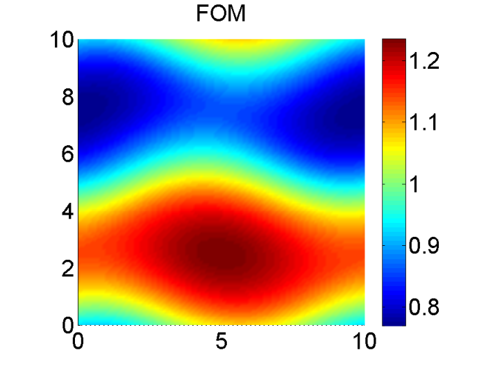
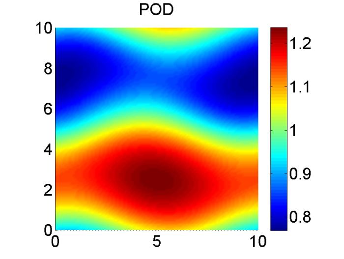
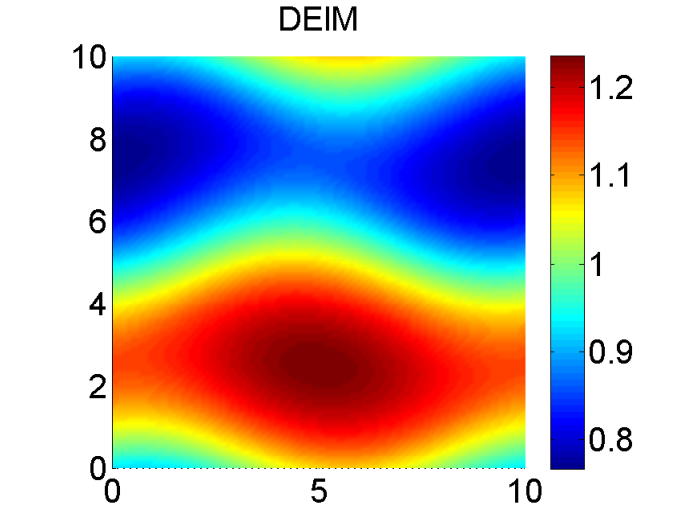
The energy and the enstrophy errors in Figure 2 show small drifts with bounded oscillations over the time, i.e. they are preserved approximately at the same level of accuracy. In Figures 3-4, the height and the potential vorticity are shown at the final time. It is seen from the Figures 3-4 and Tables 1-2 that reduced solutions, conserved reduced quantities are of an acceptable level of accuracy. The speed-up factors in Table 3 shows that the ROM with DEIM increases the computational efficiency further.


5.2 Single-layer shear instability
We consider the NTSWE on the periodic spatial domain and on the time interval [37]. The initial conditions are given as
where , and the dimensionless spatial domain length , as the case in the first test example. This problem illustrates the roll-up of an unstable shear layer.
In this test example, each snapshot matrix , and has sizes , and the number of POD and DEIM modes are set as and , respectively, according to the energy criteria (15).
The energy and enstropy errors in Figure 5 are bounded over time with small oscillations as in the case of the first test example. Similarly, the height and the potential vorticity are well approximated by the ROMs at the final time in Figures 6-7. In Tables 1-2 and Table 3, the accuracy and computational efficiency of the reduced approximations are demonstrated.


| Example 5.1 | 30 POD modes | 1.346e-01 | 1.346e-01 | 7.261e-03 |
| 200 DEIM modes | 1.370e-01 | 1.370e-01 | 7.368e-03 | |
| Example 5.2 | 18 POD modes | 2.467e-03 | 9.512e-03 | 2.598e-04 |
| 170 DEIM modes | 3.902e-03 | 1.606e-02 | 4.567e-04 |
6 Conclusions
In contrast to the canonical Hamiltonian systems like the NLS and non-canonical Hamiltonian systems with constant Poisson structure, NTSWE possesses state dependent Poisson structure. In this paper, the Hamiltonian/energy reduced order modeling approach in [21] is applied by reducing further the computational cost of the ROM in the online stage by exploiting the special structure of the skew-symmetric matrix corresponding to the discretized Poisson structure. The accuracy and computational efficiency of the reduced solutions are demonstrated by numerical examples for the POD and DEIM. Preservation of the energy and enstrophy shows further the stability of the reduced solutions over time.
Acknowledgement
This work was supported by 100/2000 Ph.D. Scholarship Program of the Turkish Higher Education Council.
References
- [1] Babak Maboudi Afkham and Jan S. Hesthaven. Structure preserving model reduction of parametric Hamiltonian systems. SIAM Journal on Scientific Computing, 39(6):A2616–A2644, 2017.
- [2] P. Astrid, S. Weiland, K. Willcox, and T. Backx. Missing point estimation in models described by proper orthogonal decomposition. IEEE Transactions on Automatic Control, 53(10):2237–2251, 2008.
- [3] Maxime Barrault, Yvon Maday, Ngoc Cuong Nguyen, and Anthony T. Patera. An empirical interpolation method: application to efficient reduced-basis discretization of partial differential equations. Comptes Rendus Mathematique, 339(9):667–672, 2004.
- [4] W. Bauer and C.J. Cotter. Energy-enstrophy conserving compatible finite element schemes for the rotating shallow water equations with slip boundary conditions. Journal of Computational Physics, 373:171 – 187, 2018.
- [5] Eric Belanger and Alain Vincent. Data assimilation (4d-var) to forecast flood in shallow-waters with sediment erosion. Journal of Hydrology, 300(1-4):114–125, 2005.
- [6] D. A. Bistrian and I. M. Navon. An improved algorithm for the shallow water equations model reduction: Dynamic Mode Decomposition vs POD. International Journal for Numerical Methods in Fluids, 78(9):552–580, 2015.
- [7] Diana A Bistrian and Ionel M Navon. The method of dynamic mode decomposition in shallow water and a swirling flow problem. International Journal for Numerical Methods in Fluids, 83(1):73–89, 2017.
- [8] E Boss, N Paldor, and L Thompson. Stability of a potential vorticity front: from quasi-geostrophy to shallow water. Journal of Fluid Mechanics, 315:65–84, 1996.
- [9] Kevin Carlberg, Charbel Farhat, Julien Cortial, and David Amsallem. The GNAT method for nonlinear model reduction: Effective implementation and application to computational fluid dynamics and turbulent flows. Journal of Computational Physics, 242:623–647, 2013.
- [10] Kevin Carlberg, Ray Tuminaro, and Paul Boggs. Preserving Lagrangian structure in nonlinear model reduction with application to structural dynamics. SIAM J. Sci. Comput., 37(2):B153–B184, 2015.
- [11] S. Chaturantabut, C. Beattie, and S. Gugercin. Structure-preserving model reduction for nonlinear port-Hamiltonian systems. SIAM Journal on Scientific Computing, 38(5):B837–B865, 2016.
- [12] Saifon Chaturantabut and Danny C. Sorensen. Nonlinear model reduction via discrete empirical interpolation. SIAM J. SCI. COMPUT., 32(5):2737–2764, 2010.
- [13] David Cohen and Ernst Hairer. Linear energy-preserving integrators for Poisson systems. BIT Numerical Mathematics, 51(1):91–101, 2011.
- [14] Colin J Cotter and Jemma Shipton. Mixed finite elements for numerical weather prediction. Journal of Computational Physics, 231(21):7076–7091, 2012.
- [15] Răzvan Ştefănescu and Ionel M. Navon. POD/DEIM nonlinear model order reduction of an ADI implicit shallow water equations model. Journal of Computational Physics, 237:95 – 114, 2013.
- [16] Răzvan Ştefănescu, Adrian Sandu, and Ionel M. Navon. Comparison of pod reduced order strategies for the nonlinear 2D shallow water equations. International Journal for Numerical Methods in Fluids, 76(8):497–521, 2014.
- [17] Paul J. Dellar and Rick Salmon. Shallow water equations with a complete coriolis force and topography. Physics of Fluids, 17(10):106601, 2005.
- [18] Christopher Eldred, Thomas Dubos, and Evaggelos Kritsikis. A quasi-Hamiltonian discretization of the thermal shallow water equations. Journal of Computational Physics, 379:1 – 31, 2019.
- [19] Vahid Esfahanian and Khosro Ashrafi. Equation-free/Galerkin-free reduced-order modeling of the shallow water equations based on Proper Orthogonal Decomposition. Journal of Fluids Engineering, 131(7):071401–071401–13, 2009.
- [20] Theo Gerkema and Victor I Shrira. Near-inertial waves in the ocean: beyond the ‘traditional approximation’. Journal of Fluid Mechanics, 529:195–219, 2005.
- [21] Yuezheng Gong, Qi Wang, and Zhu Wang. Structure-preserving galerkin POD reduced-order modeling of Hamiltonian systems. Computer Methods in Applied Mechanics and Engineering, 315:780 – 798, 2017.
- [22] Bülent Karasözen and Murat Uzunca. Energy preserving model order reduction of the nonlinear schrödinger equation. Advances in Computational Mathematics, 44(6):1769–1796, 2018.
- [23] Sanjay Lall, Petr Krysl, and Jerrold E. Marsden. Structure-preserving model reduction for mechanical systems. Phys. D, 184(1-4):304–318, 2003.
- [24] S Leibovich and SK Lele. The influence of the horizontal component of earth’s angular velocity on the instability of the ekman layer. Journal of Fluid Mechanics, 150:41–87, 1985.
- [25] Alexander Lozovskiy, Matthew Farthing, and Chris Kees. Evaluation of Galerkin and Petrov-Galerkin model reduction for finite element approximations of the shallow water equations. Computer Methods in Applied Mechanics and Engineering, 318:537 – 571, 2017.
- [26] Alexander Lozovskiy, Matthew Farthing, Chris Kees, and Eduardo Gildin. POD-based model reduction for stabilized finite element approximations of shallow water flows. Journal of Computational and Applied Mathematics, 302:50 – 70, 2016.
- [27] Peter Lynch. Hamiltonian methods for geophysical fluid dynamics: An introduction, 2002.
- [28] John Marshall and Friedrich Schott. Open-ocean convection: Observations, theory, and models. Reviews of Geophysics, 37(1):1–64, 1999.
- [29] Yuto Miyatake. Structure-preserving model reduction for dynamical systems with a first integral. Japan Journal of Industrial and Applied Mathematics, 36(3):1021–1037, 2019.
- [30] N. C. Nguyen, A. T. Patera, and J. Peraire. A ”best points” interpolation method for efficient approximation of parametrized functions. International Journal for Numerical Methods in Engineering, 73(4):521–543, 2008.
- [31] Mario Ohlberger and Stephan Rave. Reduced basis methods: Success, limitations and future challenges. Proceedings of the Conference Algoritmy, pages 1–12, 2016.
- [32] Liqian Peng and Kamran Mohseni. Symplectic model reduction of Hamiltonian systems. SIAM Journal on Scientific Computing, 38(1):A1–A27, 2016.
- [33] R Salmon. Hamiltonian fluid mechanics. Annual Review of Fluid Mechanics, 20(1):225–256, 1988.
- [34] Rick Salmon. Poisson-bracket approach to the construction of energy- and potential-enstrophy-conserving algorithms for the shallow-water equations. Journal of the Atmospheric Sciences, 61(16):2016–2036, 2004.
- [35] Andrew L. Stewart and Paul J. Dellar. Multilayer shallow water equations with complete Coriolis force. part 1. derivation on a non-traditional beta-plane. Journal of Fluid Mechanics, 651:387–413, 2010.
- [36] Andrew L Stewart and Paul J Dellar. Multilayer shallow water equations with complete coriolis force. part 3. hyperbolicity and stability under shear. Journal of Fluid Mechanics, 723:289–317, 2013.
- [37] Andrew L. Stewart and Paul J. Dellar. An energy and potential enstrophy conserving numerical scheme for the multi-layer shallow water equations with complete Coriolis force. Journal of Computational Physics, 313:99 – 120, 2016.
- [38] Geoffrey K Vallis. Atmospheric and oceanic fluid dynamics. Cambridge University Press, 2017.
- [39] Emma S Warneford and Paul J Dellar. Thermal shallow water models of geostrophic turbulence in jovian atmospheres. Physics of Fluids, 26(1):016603, 2014.
- [40] Golo Wimmer, Colin Cotter, and Werner Bauer. Energy conserving upwinded compatible finite element schemes for the rotating shallow water equations. arXiv e-prints, 2019.
- [41] R. Zimmermann and K. Willcox. An accelerated greedy missing point estimation procedure. SIAM Journal on Scientific Computing, 38(5):A2827–A285, 2016.