跳到论文正文
W Papers独立论文阅读器 arXiv:2002.11673 论文正文 计算阅读时间 · 0%
引用这篇论文根据当前论文元数据生成,正式投稿前建议核对。


License: arXiv.org perpetual non-exclusive license
arXiv:2002.11673v1 [math.NA] 26 Feb 2020

A corrected decoupled scheme for chemotaxis modelsJournal: arXiv

M. Akhmouch    M. Benzakour Amine Email: benzakouramine.m@ucd.ac.ma Address:  Département de Mathématiques, Faculté des sciences et techniques de Fès, USMBA, B.P. 2202 Fès, Maroc Corresponding author: Corresponding author
Abstract

The main purpose of this paper is to present a new corrected decoupled scheme combined with a spatial finite volume method for chemotaxis models. First, we derive the scheme for a parabolic-elliptic chemotaxis model arising in embryology. We then establish the existence and uniqueness of the numerical solution, and we prove that it converges to a corresponding weak solution for the studied model. In the last section, several numerical tests are presented by applying our approach to a number of chemotaxis systems. The obtained numerical results demonstrate the efficiency of the proposed scheme and its effectiveness to capture different forms of spatial patterns.

Keywords: 
Chemotaxis , Decoupled scheme , Correction term , Time discretization
2010 MSC
65M08 , 65M12 , 92C17 .

1 Introduction

Chemotaxis refers to a phenomenon that enables cells (or organisms) to migrate in response to a chemical signal. This process has sparked the interest of many scientists since it is encountered in several medical and biological applications, such as bacteria aggregation, tumour growth, integumental patterns in animals etc.

In [7], Oster and Murray discussed a cell-chemotaxis model involving motile cells that respond to a chemoattractant secreted by the cells themselves. In its dimensionless form, the model reads

{∂tu=μΔu−a∇⋅(u∇c),∂tc=Δ​c+uu+1−c,\left\{\begin{aligned} &\partial_{t}u=\mu\Delta u-a\nabla\cdot(\,u\nabla c),\\ &\partial_{t}c=\Delta c+\frac{u}{u+1}-c\,,\end{aligned}\right. (1.1)

where μ\mu and aa are positive constants, uu is the cell density and cc is the concentration of chemoattractant.

The above system is based on the Keller-Segel model [8], which is the most popular model for chemotaxis. The migration of cells is assumed to be governed by Fickian diffusion and chemotaxis, and the mass of cells is conserved. The chemoattractant is assumed also to diffuse, but it increases with cell density in Michaelis-Menten way and undergoes decay through simple degradation.

In [9], Murray et al. suggest that the presented cell-chemotaxis model is an appropriate mechanism for the formation of stripe patterns on the dorsal integument of embryonic and hatchling alligators (Alligator mississippiensis). These skin pigment patterns is associated with the density of melanocyte cells: Melanocytes are abundant in the regions where the black stripes appear, and are insufficient in the regions of the white stripes. The formation of these stripes is a result of a chemoattractant secretion. The system (1.1) is known to produce propagating pattern of standings peaks and troughs in cell density in the case of one-dimensional space. This patterning process was numerically and analytically investigated by Myerscough and Murray in [10].

In this paper, we will first focus on the following parabolic-elliptic system

{∂tu=μΔu−a∇⋅(u∇c)inΩT,0=Δ​c+uu+1−cin​ΩT,\left\{\begin{aligned} &\partial_{t}u=\mu\Delta u-a\nabla\cdot(\,u\nabla c)\quad\text{in}\ \Omega_{T},\\ &0=\Delta c+\frac{u}{u+1}-c\quad\text{in}\ \Omega_{T},\end{aligned}\right. (1.2)

with the homogeneous Neumann boundary and initial conditions

∇u⋅ν=∇c⋅ν=0on∂Ω×(0,Tf),u(.,0)=u0inΩ,\nabla u\cdot\nu=\nabla c\cdot\nu=0\quad\text{on}\ \partial\Omega\times(0,T_{f}),\quad u(.,0)=u_{0}\quad\text{in}\ \Omega, (1.3)

where ΩT:=Ω×(0,Tf)\Omega_{T}:=\Omega\times(0,T_{f}), Ω⊂ℝ2\Omega\subset\mathbb{R}^{2} is an open bounded polygonal subset, Tf>0T_{f}>0 is a fixed time and ν\nu denotes the outward unit-normal on the boundary ∂Ω\partial\Omega. The system (1.2) is a simpler version of the original model (1.1) in which the second equation of the system is elliptic, using the reasonable assumption that the chemoattractant diffuses much faster than cells.

In this work, we develop a decoupled finite volume scheme which can be applied to a class of chemotaxis models. For the convection-diffusion term, the approximation used is quite similar to the hybrid scheme of Spalding [20]. Concerning the time discretization, which is the main aim of this paper, it is developed such that the scheme only requires to solve decoupled systems, which excludes fully implicit discretizations. We require also that the scheme converges without needing to fulfill any CFL condition, which is not the case of the fully explicit schemes. In the literature, a number of decoupled methods for the Keller-Segel model and its variants have been proposed (see, e.g., [13, 12, 14, 4, 17, 16, 2, 3]). In all these works, the time discretization is based on the classical backward Euler scheme with an explicit approximation of some terms to avoid coupling of the system. However, it is well known that the main drawback of this strategy is its lack of accuracy. A more efficient approach will be presented in this work.

This paper provides also a convergence analysis of the proposed scheme applied to the system (1.2)–(1.3). It is proved that the convergence of the approximate solution can be obtained for any nonnegative initial cell density u0∈L2​(Ω)u_{0}\in L^{2}(\Omega). Our proof uses some techniques from [15], where a fully implicit upwind finite volume scheme is studied for the classical Keller-Segel model.

The outline of this paper is as follows. In the next section, we present our corrected decoupled finite volume scheme to approximate the solution of (1.2)–(1.3). In section 3, we prove the existence and uniqueness of the solution of the proposed scheme. Positivity preservation and mass conservation are also shown in this section. A priori estimates are given in Section 4. In Section 5, we use these estimates to prove that the approximate solution converges to a weak solution of the studied model. In Section 6, we present some numerical tests and compare the accuracy of our approach with that of more usual decoupled schemes. The paper ends with a conclusion.

2 Presentation of the numerical scheme

2.1 Spatial discretization of Ω\Omega, definitions and preliminaries

We assume that Ω⊂ℝ2\Omega\subset\mathbb{R}^{2} is an open bounded polygonal subset. Following Definition 9.1 in [18], we consider an admissible finite volume mesh of Ω\Omega, denoted by 𝒯\mathcal{T}. This mesh is given by:

  • ∙\bullet

    A family of control volumes which is commonly denoted by the same notation of the mesh 𝒯\mathcal{T}. All control volumes are open and convex polygons.

  • ∙\bullet

    A family ℰ\mathcal{E} of edges , where the set of edges of any control volume K∈𝒯K\in\mathcal{T} is denoted by ℰK\mathcal{E}_{K}. We denote also by σ=K|L\sigma=K|L the edge between KK and LL (σ∈ℰK\sigma\in\mathcal{E}_{K} and σ∉∂Ω\sigma\notin\partial\Omega).

  • ∙\bullet

    A family of points (xK)K∈𝒯(x_{K})_{K\in\mathcal{T}} such that xK∈K¯x_{K}\in\overline{K} (for all K∈𝒯K\in\mathcal{T}). The straight line going through xKx_{K} and xLx_{L} must be orthogonal to σ=K|L\sigma=K|L.

For all KK ∈𝒯\in\mathcal{T}, we denote by 𝒩⁡(K)\mathcal{N}(K) the set of control volumes which have a common edge with KK, and by m the Lebesgue measure in ℝ2\mathbb{R}^{2} or ℝ\mathbb{R}.

For all σ∈ℰK\sigma\in\mathcal{E}_{K}, we define

dσ={d​(xK,σ)if ​σ⊂∂Ω,d​(xK,xL)otherwise ,σ=K|L,d_{\sigma}=\left\{\begin{array}[]{ll}\text{\rm d}(x_{K},\sigma)&\quad\mbox{if }\sigma\subset\partial\Omega,\\ \text{\rm d}(x_{K},x_{L})&\quad\mbox{otherwise },\ \sigma=K|L,\end{array}\right.

where d is the Euclidean distance, and we denote by τσ\tau_{\sigma} the transmissibility coefficient given by:

τσ=m​(σ)dσ,σ∈ℰ.\tau_{\sigma}=\frac{\text{\rm m}(\sigma)}{d_{\sigma}},\quad\sigma\in\mathcal{E}.

The time discretization of (0,Tf)(0,T_{f}) is given by a uniform partition: 0=t0<t1<…<tN=Tf0=t_{0}<t_{1}<...<t_{N}=T_{f} with N∈ℕN\in\mathbb{N} and tn=n​Δ​tt_{n}=n\Delta t for n=0,…,Nn=0,...,N.

We denote by hh the maximal size (diameter) of the control volumes included in 𝒯\mathcal{T}, and we define

δ=max​(Δ​t,h).\delta=\text{max}(\Delta t,h).

In Section 4, the following time-step condition will be used: there exists α>0\alpha>0 such that

1−2​a​Δ​t≥α.1-2a\Delta t\geq\alpha. (2.1)

We will also need this additional constraint on the mesh: there exists ξ>0\xi>0 such that

d​(xK,σ)≥ξ​d​(xK,xL),\text{\rm d}(x_{K},\sigma)\geq\xi\,\text{\rm d}(x_{K},x_{L}), (2.2)

which is specially needed to apply the discrete Gagliardo-Nirenberg-Sobolev inequality (see Lemma 2.1).

We define a weak solution of the system (1.2) with boundary and initial conditions (1.3) as follows:

Definition 2.1.

A weak solution of the initial-boundary value problem (1.2)–(1.3) is a pair of functions (u,c)∈L2​(0,T,H1​(Ω))2(u,c)\in L^{2}(0,T;H^{1}(\Omega))^{2} which verify the following identities for all test functions ψ∈𝒟⁡(Ω×[0,Tf))\psi\in\mathcal{D}(\Omega\times[0,T_{f})) :

∫0T∫Ω(u∂tψ−μ∇u⋅∇ψ+au∇c⋅∇ψ)dxdt+∫Ωu0ψ(x,0)dx=0,\displaystyle\int_{0}^{T}\int_{\Omega}\left(u\,\partial_{t}\psi-\mu\nabla u\cdot\nabla\psi+a\,u\nabla c\cdot\nabla\psi\right)\,dxdt+\int_{\Omega}u_{0}\,\psi(x,0)\,dx=0, (2.3)
∫0T∫Ω∇c⋅∇ψ​𝑑x​𝑑t=∫0T∫Ω(uu+1−c)​ψ​𝑑x​𝑑t.\displaystyle\int_{0}^{T}\int_{\Omega}\nabla c\cdot\nabla\psi\ dxdt=\int_{0}^{T}\int_{\Omega}\left(\frac{u}{u+1}-c\right)\psi\,dxdt.\, (2.4)

We denote by X⁡(𝒯)X(\mathcal{T}) the set of functions from Ω\Omega to ℝ\mathbb{R} which are constant over each control volume of the mesh. Let 1≤p<∞1\leq p<\infty, if v∈X⁡(𝒯)v\in X(\mathcal{T}), the corresponding discrete LpL^{p} norm reads

‖v‖p=(∑K∈𝒯m​(K)​|vK|p)1/p,\|\,v\,\|_{p}=\left(\sum_{K\in\mathcal{T}}\text{\rm m}(K)\,|v_{K}|^{p}\right)^{1/p},

where v⁡(x)=vKv(x)=v_{K} for all x∈Kx\in K and for all K∈𝒯K\in\mathcal{T}. We define also the discrete W1,pW^{1,p} seminorm and the discrete W1,pW^{1,p} norm:

|v|1,p,𝒯=(∑σ∈ℰm​(σ)dσp−1​|Dσ​v|p)1/p,|\,v\,|_{1,p,\mathcal{T}}=\left(\sum_{\sigma\in\mathcal{E}}\frac{\text{\rm m}(\sigma)}{d_{\sigma}^{p-1}}\,|D_{\sigma}v|^{p}\right)^{1/p},
‖v‖1,p,𝒯=‖v‖p+|v|1,p,𝒯,\|\,v\,\|_{1,p,\mathcal{T}}=\|\,v\,\|_{p}+|\,v\,|_{1,p,\mathcal{T}}\,,

where for all σ∈ℰ\sigma\in\mathcal{E}, Dσ​v=0D_{\sigma}v=0 if σ⊂∂Ω\sigma\subset\partial\Omega and Dσ​v=|vK−vL|D_{\sigma}v=|v_{K}-v_{L}| otherwise, with σ=K|L\sigma=K|L.

We now recall the discrete Gagliardo-Nirenberg-Sobolev inequality (see [19]), which will be useful to establish a priori estimates in Section 4.

Lemma 2.1.

Let Ω\Omega be a an open bounded polyhedral domain of ℝd\mathbb{R}^{d}, d≥2d\geq 2. Let 𝒯\mathcal{T} a mesh satisfying (2.2) and v∈X⁡(𝒯)v\in X(\mathcal{T}).

  • ∙\bullet

    If 1≤p<d1\leq p<d, let 1≤s≤r≤p∗=p​d/(d−p),1\leq s\leq r\leq p^{*}=pd/(d-p),

  • ∙\bullet

    If p≥dp\geq d, let 1≤s≤r<+∞.1\leq s\leq r<+\infty.

Then there exists a constant C>0C>0 only depending on p,s,r,dp,s,r,d and Ω\Omega such that

‖v‖r≤Cξ(p−1)​θ/p​‖v‖1,p,𝒯θ​‖v‖s1−θ,∀v∈X⁡(𝒯),\|\,v\,\|_{r}\,\leq\,\frac{C}{\xi^{(p-1)\theta/p}}\,\,\|\,v\,\|^{\theta}_{1,p,\mathcal{T}}\,\|\,v\,\|_{s}^{1-\theta},\ \forall v\in X(\mathcal{T}),

where θ\theta is defined by

θ=1/s−1/r1/s+1/d−1/p.\theta=\dfrac{1/s-1/r}{1/s+1/d-1/p}.

2.2 The corrected decoupled finite volume scheme

We begin this section by presenting a classical decoupled finite volume scheme for the problem (1.2)–(1.3):

for all K∈𝒯K\in\mathcal{T} and n=0,…,N−1n=0,...,N-1

m​(K)​uKn+1−uKnΔ​t−μ​∑σ∈ℰKτσ​D​uK,σn+1\displaystyle\text{\rm m}(K)\frac{u^{n+1}_{K}-u^{n}_{K}}{\Delta t}-\mu\sum_{\sigma\in\mathcal{E}_{K}}\tau_{\sigma}Du_{K,\sigma}^{n+1}
+a∑σ∈ℰKσ=K|Lτσ(S(DcK,σn+1)uKn+1−S(−DcK,σn+1)uLn+1)=0,\displaystyle+a\sum_{\begin{subarray}{c}\sigma\in\mathcal{E}_{K}\\ \sigma=K|L\end{subarray}}\tau_{\sigma}\left(S\left(Dc_{K,\sigma}^{n+1}\right)u_{K}^{n+1}-S\left(-Dc_{K,\sigma}^{n+1}\right)u_{L}^{n+1}\right)=0, (2.5)
−∑σ∈ℰKτσDcK,σn+1+m(K)cKn+1=m(K)uKnuKn+1,\displaystyle-\sum_{\sigma\in\mathcal{E}_{K}}\tau_{\sigma}\,Dc^{n+1}_{K,\sigma}+\text{\rm m}(K)\,c_{K}^{n+1}=\text{\rm m}(K)\,\frac{u_{K}^{n}}{u_{K}^{n}+1}, (2.6)

with the compatible initial condition

uK0=1m​(K)​∫Ku0​(x)​𝑑x,u^{0}_{K}=\frac{1}{\text{\rm m}(K)}\int_{K}u_{0}(x)\,dx, (2.7)

and where for all σ∈ℰK\sigma\in\mathcal{E}_{K}

D​vK,σn={0for ​σ⊂∂Ω,vLn−vKnotherwise ,σ=K|L.Dv_{K,\sigma}^{n}=\left\{\begin{array}[]{ll}0&\quad\mbox{for }\sigma\subset\partial\Omega,\\ v_{L}^{n}-v_{K}^{n}&\quad\mbox{otherwise },\ \sigma=K|L.\end{array}\right.\\

In the above scheme, the function SS is defined by

S⁡(x)={0,if ​x<2​(−μ+ε)/a,x2,if ​|x|≤2​(μ−ε)/a,x,if ,x>2​(μ−ε)/a,S(x)=\left\{\begin{array}[]{ll}0,&\quad\mbox{if }x<2\left(-\mu+\varepsilon\right)/a,\\ \dfrac{x}{2},&\quad\mbox{if }|x|\leq 2\left(\mu-\varepsilon\right)/a,\\ x,&\quad\mbox{if },x>2\left(\mu-\varepsilon\right)/a,\end{array}\right.\\ (2.8)

where ε\varepsilon is a small constant such that ε≥0\varepsilon\geq 0 and ε<<μ\varepsilon<<\mu.

The terms uKnu^{n}_{K} and cKnc^{n}_{K} denote respectively the approximations of the quantities 1m​(K)​∫Ku⁡(x,tn)​𝑑x\frac{1}{\text{\rm m}(K)}\int_{K}u(x,t^{n})\,dx and 1m​(K)​∫Kc⁡(x,tn)​𝑑x\frac{1}{\text{\rm m}(K)}\int_{K}c(x,t^{n})\,dx. As we can see, the proposed finite volume scheme is decoupled: at each time-step, we begin by solving (2.6) to compute cKn+1c^{n+1}_{K} and then, we compute uKn+1u^{n+1}_{K} from (2.5). The discretization used for ∇⋅(u∇c)\nabla\cdot(u\nabla c) is equivalent to the second order central difference scheme when |D​cK,σn+1|≤2​(μ−ε)/a\left|Dc_{K,\sigma}^{n+1}\right|\leq 2\left(\mu-\varepsilon\right)/a and to the first order upwind scheme when D​cK,σn+1<2​(−μ+ε)/aDc_{K,\sigma}^{n+1}<2\left(-\mu+\varepsilon\right)/a or D​cK,σn+1>2​(μ−ε)/aDc_{K,\sigma}^{n+1}>2\left(\mu-\varepsilon\right)/a. When ε=0\varepsilon=0, the scheme is identical to that of Spalding [20] (see also [11]).

It is clear that we can obtain a best accuracy if we replace (2.6) by the equation

−∑σ∈ℰKτσDcK,σn+1+m(K)cKn+1=m(K)uKn+1uKn+1+1,-\sum_{\sigma\in\mathcal{E}_{K}}\tau_{\sigma}\,Dc^{n+1}_{K,\sigma}+\text{\rm m}(K)\,c_{K}^{n+1}=\text{\rm m}(K)\,\frac{u_{K}^{n+1}}{u_{K}^{n+1}+1}, (2.9)

however, it will be expensive in term of computational cost to find the solution of the scheme (2.5),(2.9) since we have to solve a large nonlinear system at each time step.

Now, for all K∈𝒯K\in\mathcal{T} and n=0,…,N−1n=0,...,N-1, we define

TKn+1=m​(K)​(uKn+1uKn+1+1−uKnuKn+1),TK0=0.T_{K}^{n+1}=\text{\rm m}(K)\left(\frac{u_{K}^{n+1}}{u_{K}^{n+1}+1}-\frac{u_{K}^{n}}{u_{K}^{n}+1}\right),\quad T_{K}^{0}=0. (2.10)

The equation (2.9) can then be written as

−∑σ∈ℰKτσDcK,σn+1+m(K)cKn+1=m(K)uKnuKn+1+TKn+1.-\sum_{\sigma\in\mathcal{E}_{K}}\tau_{\sigma}\,Dc^{n+1}_{K,\sigma}+\text{\rm m}(K)\,c_{K}^{n+1}=\text{\rm m}(K)\,\frac{u_{K}^{n}}{u_{K}^{n}+1}+T_{K}^{n+1}. (2.11)

As we can see, the only difference between (2.11) and (2.6) is the term TKn+1T_{K}^{n+1}, so we conjecture that we can improve the accuracy of the decoupled scheme (2.5)–(2.6) if we add to the right hand side of (2.6) a correction term which approximates TKn+1T_{K}^{n+1}. Hence, we propose to replace (2.6) with the following scheme:

−∑σ∈ℰKτσDcK,σn+1+m(K)cKn+1=m(K)uKnuKn+1+βnTKn,-\sum_{\sigma\in\mathcal{E}_{K}}\tau_{\sigma}\,Dc^{n+1}_{K,\sigma}+\text{\rm m}(K)\,c_{K}^{n+1}=\text{\rm m}(K)\,\frac{u_{K}^{n}}{u_{K}^{n}+1}+\beta_{n}T_{K}^{n}, (2.12)

where βn>0\beta_{n}>0. The purpose of βn\beta_{n} is to ensure the nonnegativity of the right-hand side of (2.12), to do not affect the nonnegativity of cKn+1c^{n+1}_{K}. Then, by supposing that uKn≥0u_{K}^{n}\geq 0 (this will be proved in Section 3), we define βn\beta_{n} for n=0,…,N−1n=0,...,N-1 as follows:

βn={1,if ​𝒯n∗=∅,minK∈𝒯n∗​uKnuKn+1uKn−1uKn−1+1−uKnuKn+1,otherwise ,\beta_{n}=\left\{\begin{array}[]{ll}1,&\quad\mbox{if }\mathcal{T}^{*}_{n}=\emptyset,\\ \underset{{K\in\mathcal{T}^{*}_{n}}}{\text{min}}\cfrac{\cfrac{u_{K}^{n}}{u_{K}^{n}+1}}{\cfrac{u_{K}^{n-1}}{u_{K}^{n-1}+1}-\cfrac{u_{K}^{n}}{u_{K}^{n}+1}},&\quad\mbox{otherwise },\\ \end{array}\right.\\ (2.13)

where 𝒯n∗={K∈𝒯| 2​uKnuKn+1−uKn−1uKn−1+1<0}\mathcal{T}^{*}_{n}=\left\{K\in\mathcal{T}\,\middle|\,2\cfrac{u_{K}^{n}}{u_{K}^{n}+1}-\cfrac{u_{K}^{n-1}}{u_{K}^{n-1}+1}<0\right\} for n=0,…,N−1n=0,...,N-1 and 𝒯0∗=∅\mathcal{T}^{*}_{0}=\emptyset. We can easily verify that 0<βn≤10<\beta_{n}\leq 1. We mention however that, in practice, we will take βn=1\beta_{n}=1, which seems the most natural choice. Indeed, several numerical tests are performed and, as expected, the right-hand side of (2.12) is always positive for this value unless the time-step size is extremely large.

We define uδ,cδu_{\delta},\>c_{\delta}, the finite volume approximations of uu and cc by:

uδ​(x,t)=uKn+1,cδ​(x,t)=cKn+1,x∈K,t∈[tn,tn+1).u_{\delta}(x,t)=u^{n+1}_{K},\quad c_{\delta}(x,t)=c^{n+1}_{K},\quad x\in K,\,t\in[t^{n},t^{n+1}). (2.14)

We define also approximations of the gradients of uu and cc. To this end, we begin by defining MK,σM_{K,\sigma}, which is the cell formed from the vertices of σ\sigma, xKx_{K} and xLx_{L} if σ=K|L⊄∂Ω\sigma=K|L\not\subset\partial\Omega, and from the vertices of σ\sigma and xKx_{K} if σ⊂∂Ω\sigma\subset\partial\Omega.

Following [6], we define the discrete gradient d​vδdv_{\delta} which is the approximation of ∇v\nabla v by

d​vδ​(x,t)=m​(σ)m​(MK,σ)​D​vK,σn+1​νK,σ,x∈MK,σ,t∈(tn,tn+1),\displaystyle dv_{\delta}(x,t)=\frac{\text{\rm m}(\sigma)}{\text{\rm m}(M_{K,\sigma})}\,Dv_{K,\sigma}^{n+1}\,\,\nu_{K,\sigma},\quad x\in M_{K,\sigma},\ t\in(t^{n},t^{n+1}),

for all K∈𝒯K\in\mathcal{T} and n=0,…,N−1n=0,...,N-1, where νK,σ\nu_{K,\sigma} denotes the unit normal on σ\sigma which is outward to KK.

3 Existence and uniqueness of a discrete solution

In this section, we prove existence and uniqueness of the solution of the proposed scheme. We show also that the scheme is mass conserving and positivity preserving.

Proposition 3.1.

Assume that u0≥0u_{0}\geq 0. Then there exists a unique solution {(uKn+1,cKn+1),K∈𝒯,n=0,…,N−1}\{(u_{K}^{n+1},c_{K}^{n+1}),\,K\in\mathcal{T},\,n=0,...,N-1\} to the scheme (2.5),(2.12) which satisfies the following properties :

uKn+1≥0andcKn+1≥0for all​K∈𝒯,n=0,…,N−1,\displaystyle u_{K}^{n+1}\geq 0\quad\text{and}\quad c_{K}^{n+1}\geq 0\quad\text{for all}\ K\in\mathcal{T},\,n=0,...,N-1, (3.1)
∑K∈𝒯m(K)uKn+1=∑K∈𝒯m(K)uK0=∥u0∥L1​(Ω),for all n=0,…,N−1.\displaystyle\sum_{K\in\mathcal{T}}\text{\rm m}(K)\,u_{K}^{n+1}=\sum_{K\in\mathcal{T}}\text{\rm m}(K)\,u_{K}^{0}=\|u_{0}\|_{L^{1}(\Omega)},\quad\text{for all }n=0,...,N-1. (3.2)
Proof.

For all n=0,…,N−1n=0,...,N-1, we define the vectors Un+1=(UKn+1)K∈𝒯U^{n+1}=\left(U^{n+1}_{K}\right)_{K\in\mathcal{T}}, Fn=(FKn)K∈𝒯F^{n}=\left(F^{n}_{K}\right)_{K\in\mathcal{T}}, Cn+1=(CKn+1)K∈𝒯C^{n+1}=\left(C^{n+1}_{K}\right)_{K\in\mathcal{T}} and Gn=(GKn)K∈𝒯G^{n}=\left(G^{n}_{K}\right)_{K\in\mathcal{T}}, for which:

UKn+1=uKn+1,FKn=m​(K)​uKn/Δ​t,\displaystyle U_{K}^{n+1}=u_{K}^{n+1},\quad F_{K}^{n}=\text{\rm m}(K)u_{K}^{n}/\Delta t,
CKn+1=cKn+1,GKn=m​(K)​uKnuKn+1+βn​TKn.\displaystyle C_{K}^{n+1}=c_{K}^{n+1},\quad G_{K}^{n}=\text{\rm m}(K)\frac{u_{K}^{n}}{u_{K}^{n}+1}+\beta_{n}T_{K}^{n}.

We also define the matrix An=(AK,Kn)K∈𝒯A^{n}=\left(A_{K,K}^{n}\right)_{K\in\mathcal{T}} and B=(BK,K)K∈𝒯B=\left(B_{K,K}\right)_{K\in\mathcal{T}} by

AK,Kn=m​(K)/Δ​t+∑σ∈ℰKσ⊄∂Ωτσ​(μ+a​S​(D​cK,σn+1)),AK,Ln=−τσ(μ+aS(−DcK,σn+1)),ifL∈𝒩(K) with σ=K|L,AK,Ln=0,otherwise,andBK,K=∑σ∈ℰKσ⊄∂Ωτσ+m​(K),BK,L=−τσ,ifL∈𝒩(K) with σ=K|L,BK,L=0,otherwise.\displaystyle\begin{aligned} &A_{K,K}^{n}=\text{\rm m}(K)/\Delta t+\sum_{\begin{subarray}{c}\sigma\in\mathcal{E}_{K}\\ \sigma\not\subset\partial\Omega\end{subarray}}\tau_{\sigma}\left(\mu+a\,S\left(Dc_{K,\sigma}^{n+1}\right)\right),\\ &A_{K,L}^{n}=-\tau_{\sigma}\left(\mu+a\,S\left(-Dc_{K,\sigma}^{n+1}\right)\right),\quad\text{if}\,L\in\mathcal{N}(K)\text{ with }\sigma=K|L,\\ &A_{K,L}^{n}=0,\quad\text{otherwise},\\ \text{and}\\ &B_{K,K}=\sum_{\begin{subarray}{c}\sigma\in\mathcal{E}_{K}\\ \sigma\not\subset\partial\Omega\end{subarray}}\tau_{\sigma}+\text{\rm m}(K),\\ &B_{K,L}=-\tau_{\sigma},\quad\text{if}\,L\in\mathcal{N}(K)\text{ with }\sigma=K|L,\\ &B_{K,L}=0,\quad\text{otherwise}.\end{aligned}

The decoupled scheme (2.5),(2.12) can be then written equivalently as

An​Un+1=Fn,\displaystyle A^{n}\,U^{n+1}=F^{n}, (3.3)
B​Cn+1=Gn.\displaystyle BC^{n+1}=G^{n}. (3.4)

To prove the desired results, we proceed by induction on nn. The proof in the case of n=0n=0 is similar to that of the inductive step. We argue now that the vectors UnU^{n} and CnC^{n} are defined and nonnegative. We have

|BK,K|−∑L∈𝒯L≠K|BK,L|=m​(K)>0,|B_{K,K}|-\sum_{\begin{subarray}{c}L\in\mathcal{T}\\ L\neq K\end{subarray}}|B_{K,L}|=\text{\rm m}(K)>0,

which means the matrix BB is strictly diagonally dominant by rows. Moreover, since the diagonal elements of BB are positive and its off-diagonal entries are nonpositive, we can conclude that BB is a nonsingular M-matrix, which implies the unique solvability of (3.4) with B−1>0B^{-1}>0 . Therefore, in view of the nonnegativity of GnG^{n} (by the definition of βn\beta_{n} (2.13)), we deduce that Cn+1≥0C^{n+1}\geq 0. Since for all σ=K|L∈ℰK\sigma=K|L\in\mathcal{E}_{K}, D​cL,σn+1=−D​cK,σn+1Dc_{L,\sigma}^{n+1}=-Dc_{K,\sigma}^{n+1}, we have for all K∈𝒯K\in\mathcal{T}

|AK,Kn|−∑L∈𝒯L≠K|AL,Kn|=m​(K)/Δ​t>0.|A_{K,K}^{n}|-\sum_{\begin{subarray}{c}L\in\mathcal{T}\\ L\neq K\end{subarray}}|A_{L,K}^{n}|=\text{\rm m}(K)/\Delta t>0.

Then AnA^{n} is strictly diagonal dominant by columns. Now, since μ+a​S​(x)≥0\mu+a\,S\left(x\right)\geq 0 for all x∈ℝx\in\mathbb{R} (by the definition (2.8)), the matrix AnA^{n} has nonpositive off-diagonal and positive diagonal entries, which implies that AnA^{n} is a nonsingular M-matrix. Consequently, the existence and uniqueness of Un+1U^{n+1} is proved, and since Fn≥0F^{n}\geq 0, it is clear that Un+1≥0U^{n+1}\geq 0.

Now, summing (2.5) over K∈𝒯K\in\mathcal{T}, we have:

∑K∈𝒯m​(K)​(uKn+1−uKn)=0.\sum_{K\in\mathcal{T}}\text{\rm m}(K)\left(u_{K}^{n+1}-u_{K}^{n}\right)=0.

Then, summing over n=0,1,…,pn=0,1,...,p, with p≤N−1p\leq N-1 we get (3.2):

∑K∈𝒯m(K)uKp+1=∑K∈𝒯m(K)uK0=∥u0∥L1​(Ω),for all p=0,…,N−1,\sum_{K\in\mathcal{T}}\text{\rm m}(K)\,u_{K}^{p+1}=\sum_{K\in\mathcal{T}}\text{\rm m}(K)\,u_{K}^{0}=\|u_{0}\|_{L^{1}(\Omega)},\quad\text{for all }p=0,...,N-1\,,

which ends the proof.

∎

4 A priori estimates

In all this section, we assume that u0∈L2​(Ω)u_{0}\in L^{2}(\Omega) and u0≥0u_{0}\geq 0. We assume also that {(uKn+1,cKn+1),K∈𝒯,n=0,…,N−1}\{\left(u_{K}^{n+1},c_{K}^{n+1}\right),\,K\in\mathcal{T},\,n=0,...,N-1\} is the solution of the scheme (2.5),(2.12).

Proposition 4.1.

For all n=0,…,N−1n=0,...,N-1 and for all K∈𝒯K\in\mathcal{T}, we have

cKn+1≤2,\displaystyle c_{K}^{n+1}\leq 2, (4.1)
∑K∈𝒯∑σ∈ℰKτσ​|D​cK,σn+1|2≤C.\displaystyle\sum_{K\in\mathcal{T}}\sum_{\sigma\in\mathcal{E}_{K}}\tau_{\sigma}\left|Dc_{K,\sigma}^{n+1}\right|^{2}\leq C. (4.2)

where CC is a positive constant which only depends on Ω\Omega.

Proof.

Let KK be the control volume which verifies cKn+1=max​{cLn+1}L∈𝒯c_{K}^{n+1}=\mbox{max}\{c_{L}^{n+1}\}_{L\in\mathcal{T}}. Multiplying the equation (2.12) by (cKn+1−2)+\left(c_{K}^{n+1}-2\right)^{+}, and using the fact that 0<βn≤10<\beta_{n}\leq 1, we get

−∑σ∈ℰKτσDcK,σn+1(cKn+1−2)+\displaystyle-\sum_{\sigma\in\mathcal{E}_{K}}\tau_{\sigma}Dc_{K,\sigma}^{n+1}\left(c_{K}^{n+1}-2\right)^{+} ≤m​(K)​(2−cKn+1)​(cKn+1−2)+,\displaystyle\leq\text{\rm m}(K)\left(2-c_{K}^{n+1}\right)\left(c_{K}^{n+1}-2\right)^{+},

it follows that

−∑σ∈ℰKτσDcK,σn+1(cKn+1−2)+≤0.\displaystyle-\sum_{\sigma\in\mathcal{E}_{K}}\tau_{\sigma}Dc_{K,\sigma}^{n+1}\left(c_{K}^{n+1}-2\right)^{+}\leq 0.

In view of the choice of KK, D​cK,σn+1≤0Dc_{K,\sigma}^{n+1}\leq 0 for all σ∈ℰK\sigma\in\mathcal{E}_{K}, which leads to

−∑σ∈ℰKτσDcK,σn+1(cKn+1−2)+≥0.-\sum_{\sigma\in\mathcal{E}_{K}}\tau_{\sigma}Dc_{K,\sigma}^{n+1}\left(c_{K}^{n+1}-2\right)^{+}\geq 0.

Hence, we deduce that (cKn+1−2)≤0\left(c_{K}^{n+1}-2\right)\leq 0. This establish (4.1).

Now, multiplying the equation (2.12) by cKn+1c_{K}^{n+1}, summing over K∈𝒯K\in\mathcal{T}, using a summation by parts and (4.1), we get

12​∑K∈𝒯∑σ∈ℰKτσ​|D​cK,σn+1|2+∑K∈𝒯m​(K)​|cKn+1|2≤4​m​(Ω),\dfrac{1}{2}\sum_{K\in\mathcal{T}}\sum_{\sigma\in\mathcal{E}_{K}}\tau_{\sigma}\left|Dc_{K,\sigma}^{n+1}\right|^{2}+\sum_{K\in\mathcal{T}}\text{\rm m}(K)\left|c_{K}^{n+1}\right|^{2}\leq 4\text{\rm m}(\Omega),

which gives (4.2).

∎

Lemma 4.1.

Assume that (2.2) is fulfilled and that ε>0\varepsilon>0 (see (2.8)). Then, there exists a constant C>0C>0 only depending on Ω\Omega, TfT_{f},u0u_{0}, aa, ε\varepsilon and ξ\xi such that

∑n=0N∑K∈𝒯Δ​t​m​(K)​|uKn|2≤C.\sum_{n=0}^{N}\sum_{K\in\mathcal{T}}\Delta t\ \text{\rm m}(K)\left|u_{K}^{n}\right|^{2}\leq C. (4.3)
Proof.

Performing the following changes of variable:

u~Kn=uKn+1for all​K∈𝒯,n=0,…,N,\tilde{u}_{K}^{n}=u_{K}^{n}+1\quad\text{for all}\ K\in\mathcal{T},\,n=0,...,N, (4.4)

and

S~​(x)=S⁡(x)+(μ−ε)/a,\tilde{S}(x)=S(x)+\left(\mu-\varepsilon\right)/a, (4.5)

and using the identity

S⁡(x)−S⁡(−x)=x,S(x)-S(-x)=x, (4.6)

the scheme (2.5) becomes

m​(K)​u~Kn+1−u~KnΔ​t−ε​∑σ∈ℰKτσ​D​u~K,σn+1\displaystyle\text{\rm m}(K)\frac{\tilde{u}^{n+1}_{K}-\tilde{u}^{n}_{K}}{\Delta t}-\varepsilon\sum_{\sigma\in\mathcal{E}_{K}}\tau_{\sigma}D\tilde{u}_{K,\sigma}^{n+1}
+a∑σ∈ℰKσ=K|Lτσ(S~(DcK,σn+1)u~Kn+1−S~(−DcK,σn+1)u~Ln+1)−a∑σ∈ℰKτσDcK,σn=0.\displaystyle+a\sum_{\begin{subarray}{c}\sigma\in\mathcal{E}_{K}\\ \sigma=K|L\end{subarray}}\tau_{\sigma}\left(\tilde{S}\left(Dc_{K,\sigma}^{n+1}\right)\tilde{u}_{K}^{n+1}-\tilde{S}\left(-Dc_{K,\sigma}^{n+1}\right)\tilde{u}_{L}^{n+1}\right)-a\sum_{\sigma\in\mathcal{E}_{K}}\tau_{\sigma}Dc_{K,\sigma}^{n}=0. (4.7)

From (2.12), using (4.1) and since 0<βn≤10<\beta_{n}\leq 1, we can easily see that

∑σ∈ℰKτσ​D​cK,σn≤3​m​(K).\sum_{\sigma\in\mathcal{E}_{K}}\tau_{\sigma}\,Dc^{n}_{K,\sigma}\leq 3\text{\rm m}(K).

Using the above inequality in (4.7), we obtain

m​(K)​u~Kn+1−u~KnΔ​t−ε​∑σ∈ℰKτσ​D​u~K,σn+1\displaystyle\text{\rm m}(K)\frac{\tilde{u}^{n+1}_{K}-\tilde{u}^{n}_{K}}{\Delta t}-\varepsilon\sum_{\sigma\in\mathcal{E}_{K}}\tau_{\sigma}D\tilde{u}_{K,\sigma}^{n+1}
≤−a∑σ∈ℰKσ=K|Lτσ(S~(DcK,σn+1)u~Kn+1−S~(−DcK,σn+1)u~Ln+1)+3am(K).\displaystyle\leq-a\sum_{\begin{subarray}{c}\sigma\in\mathcal{E}_{K}\\ \sigma=K|L\end{subarray}}\tau_{\sigma}\left(\tilde{S}\left(Dc_{K,\sigma}^{n+1}\right)\tilde{u}_{K}^{n+1}-\tilde{S}\left(-Dc_{K,\sigma}^{n+1}\right)\tilde{u}_{L}^{n+1}\right)+3a\,\text{\rm m}(K)\,.

Let us now multiply the above inequality by Δ​t​log⁡(u~Kn+1)\Delta t\,\log\left(\tilde{u}_{K}^{n+1}\right), and summing over K∈𝒯K\in\mathcal{T}, we find that

E1+E2≤E3+E4,E_{1}+E_{2}\leq E_{3}+E_{4}, (4.8)

where

E1=∑K∈𝒯m​(K)​(u~Kn+1−u~Kn)​log⁡(u~Kn+1),\displaystyle E_{1}=\sum_{K\in\mathcal{T}}\text{\rm m}(K)\left(\tilde{u}^{n+1}_{K}-\tilde{u}^{n}_{K}\right)\log\left(\tilde{u}_{K}^{n+1}\right),
E2=−ε∑K∈𝒯∑σ∈ℰKΔtτσDu~K,σn+1log(u~Kn+1),\displaystyle E_{2}=-\varepsilon\sum_{K\in\mathcal{T}}\sum_{\sigma\in\mathcal{E}_{K}}\Delta t\,\tau_{\sigma}D\tilde{u}_{K,\sigma}^{n+1}\log\left(\tilde{u}_{K}^{n+1}\right),
E3=−a∑σ∈ℰKσ=K|LΔtτσ(S~(DcK,σn+1)u~Kn+1−S~(−DcK,σn+1)u~Ln+1)log(u~Kn+1),\displaystyle E_{3}=-a\sum_{\begin{subarray}{c}\sigma\in\mathcal{E}_{K}\\ \sigma=K|L\end{subarray}}\Delta t\,\tau_{\sigma}\left(\tilde{S}\left(Dc_{K,\sigma}^{n+1}\right)\tilde{u}_{K}^{n+1}-\tilde{S}\left(-Dc_{K,\sigma}^{n+1}\right)\tilde{u}_{L}^{n+1}\right)\log\left(\tilde{u}_{K}^{n+1}\right),
E4=3​a​∑K∈𝒯Δ​t​m​(K)​log⁡(u~Kn+1).\displaystyle E_{4}=3a\sum_{K\in\mathcal{T}}\Delta t\,\text{\rm m}(K)\log\left(\tilde{u}_{K}^{n+1}\right).

From the expression of E1E_{1}, we can see that

E1=\displaystyle E_{1}= ∑K∈𝒯m​(K)​(u~Kn+1​log⁡(u~Kn+1)−u~Kn​log⁡(u~Kn))\displaystyle\sum_{K\in\mathcal{T}}\text{\rm m}(K)\left(\tilde{u}^{n+1}_{K}\log\left(\tilde{u}_{K}^{n+1}\right)-\tilde{u}^{n}_{K}\log\left(\tilde{u}_{K}^{n}\right)\right)
−∑K∈𝒯m(K)u~Kn(log(u~Kn+1)−log(u~Kn)),\displaystyle-\sum_{K\in\mathcal{T}}\text{\rm m}(K)\tilde{u}_{K}^{n}\left(\log\left(\tilde{u}_{K}^{n+1}\right)-\log\left(\tilde{u}_{K}^{n}\right)\right),

and since we have from a Taylor expansion of log\log

u~Kn​(log⁡(u~Kn+1)−log⁡(u~Kn))≤u~Kn+1−u~Kn,\tilde{u}_{K}^{n}\left(\log\left(\tilde{u}_{K}^{n+1}\right)-\log\left(\tilde{u}_{K}^{n}\right)\right)\leq\tilde{u}_{K}^{n+1}-\tilde{u}_{K}^{n},

we deduce using the mass conservation property (3.2) that

E1≥∑K∈𝒯m​(K)​(u~Kn+1​log⁡(u~Kn+1)−u~Kn​log⁡(u~Kn)).E_{1}\geq\sum_{K\in\mathcal{T}}\text{\rm m}(K)\left(\tilde{u}^{n+1}_{K}\log\left(\tilde{u}_{K}^{n+1}\right)-\tilde{u}^{n}_{K}\log\left(\tilde{u}_{K}^{n}\right)\right).

By an integration by parts on E2E_{2}, we get

E2=ε2​∑K∈𝒯∑σ∈ℰKΔ​t​τσ​D​u~K,σn+1​(log⁡(u~Ln+1)−log⁡(u~Kn+1)).E_{2}=\dfrac{\varepsilon}{2}\sum_{K\in\mathcal{T}}\sum_{\sigma\in\mathcal{E}_{K}}\Delta t\,\tau_{\sigma}D\tilde{u}_{K,\sigma}^{n+1}\left(\log\left(\tilde{u}_{L}^{n+1}\right)-\log\left(\tilde{u}_{K}^{n+1}\right)\right).

Then, by a Taylor expansion of log\log we get

E2=ε2​∑K∈𝒯∑σ∈ℰKΔ​t​τσ​|D​u~K,σn+1θσn+1|2,E_{2}=\dfrac{\varepsilon}{2}\sum_{K\in\mathcal{T}}\sum_{\sigma\in\mathcal{E}_{K}}\Delta t\,\tau_{\sigma}\left|\dfrac{D\tilde{u}_{K,\sigma}^{n+1}}{\sqrt{\theta_{\sigma}^{n+1}}}\right|^{2},

where θσn+1=tσ​u~Kn+1+(1−tσ)​u~Ln+1\theta_{\sigma}^{n+1}=t_{\sigma}\tilde{u}_{K}^{n+1}+\left(1-t_{\sigma}\right)\tilde{u}_{L}^{n+1} with tσ∈(0,1)t_{\sigma}\in(0,1). Hence, using the fact that

|D​u~K,σn+1|θσn+1=u~Kn+1+u~Ln+1θσn+1​|D​(u~n+1)K,σ|≥|D​(u~n+1)K,σ|,\dfrac{\left|D\tilde{u}_{K,\sigma}^{n+1}\right|}{\sqrt{\theta_{\sigma}^{n+1}}}=\dfrac{\sqrt{\tilde{u}_{K}^{n+1}}+\sqrt{\tilde{u}_{L}^{n+1}}}{\sqrt{\theta_{\sigma}^{n+1}}}\left|D\left(\sqrt{\tilde{u}^{n+1}}\right)_{K,\sigma}\right|\geq\left|D\left(\sqrt{\tilde{u}^{n+1}}\right)_{K,\sigma}\right|,

we infer that

E2≥ε2​∑K∈𝒯∑σ∈ℰKΔ​t​τσ​|D​(u~n+1)K,σ|2.E_{2}\geq\dfrac{\varepsilon}{2}\sum_{K\in\mathcal{T}}\sum_{\sigma\in\mathcal{E}_{K}}\Delta t\,\tau_{\sigma}\left|D\left(\sqrt{\tilde{u}^{n+1}}\right)_{K,\sigma}\right|^{2}.

Using a summation by parts, we obtain

E3n+1=a2​∑K∈𝒯∑σ∈ℰKσ=K|LΔ​t\displaystyle E_{3}^{n+1}=\dfrac{a}{2}\sum_{K\in\mathcal{T}}\sum_{\begin{subarray}{c}\sigma\in\mathcal{E}_{K}\\ \sigma=K|L\end{subarray}}\Delta t\, τσ​(S~​(D​cK,σn+1)​u~Kn+1−S~​(−D​cK,σn+1)​u~Ln+1)\displaystyle\tau_{\sigma}\left(\tilde{S}\left(Dc_{K,\sigma}^{n+1}\right)\tilde{u}_{K}^{n+1}-\tilde{S}\left(-Dc_{K,\sigma}^{n+1}\right)\tilde{u}_{L}^{n+1}\right)
×(log⁡(u~Ln+1)−log⁡(u~Kn+1)).\displaystyle\times\left(\log\left(\tilde{u}_{L}^{n+1}\right)-\log\left(\tilde{u}_{K}^{n+1}\right)\right).

Now, we define E~3n+1\tilde{E}_{3}^{n+1}

E~3n+1=a2​∑K∈𝒯∑σ∈ℰKσ=K|LΔ​t\displaystyle\tilde{E}_{3}^{n+1}=\dfrac{a}{2}\sum_{K\in\mathcal{T}}\sum_{\begin{subarray}{c}\sigma\in\mathcal{E}_{K}\\ \sigma=K|L\end{subarray}}\Delta t τσ​θσn+1​D​cK,σn+1​(log⁡(u~Ln+1)−log⁡(u~Kn+1)).\displaystyle\,\tau_{\sigma}\theta_{\sigma}^{n+1}Dc_{K,\sigma}^{n+1}\left(\log\left(\tilde{u}_{L}^{n+1}\right)-\log\left(\tilde{u}_{K}^{n+1}\right)\right).

Next, using the identity (4.6) and the last expression of E3n+1E_{3}^{n+1}, we can write

E3n+1−E~3n+1=\displaystyle E_{3}^{n+1}-\tilde{E}_{3}^{n+1}= a2​∑K∈𝒯∑σ∈ℰKσ=K|LΔ​t​τσ​S~​(D​cK,σn+1)​(u~Kn+1−θσn+1)\displaystyle\dfrac{a}{2}\sum_{K\in\mathcal{T}}\sum_{\begin{subarray}{c}\sigma\in\mathcal{E}_{K}\\ \sigma=K|L\end{subarray}}\Delta t\,\tau_{\sigma}\tilde{S}\left(Dc_{K,\sigma}^{n+1}\right)\left(\tilde{u}_{K}^{n+1}-\theta_{\sigma}^{n+1}\right)
×(log⁡(u~Ln+1)−log⁡(u~Kn+1))+a2​∑K∈𝒯∑σ∈ℰKσ=K|LΔ​t​τσ​S~​(−D​cK,σn+1)\displaystyle\times\left(\log\left(\tilde{u}_{L}^{n+1}\right)-\log\left(\tilde{u}_{K}^{n+1}\right)\right)+\dfrac{a}{2}\sum_{K\in\mathcal{T}}\sum_{\begin{subarray}{c}\sigma\in\mathcal{E}_{K}\\ \sigma=K|L\end{subarray}}\Delta t\,\tau_{\sigma}\tilde{S}\left(-Dc_{K,\sigma}^{n+1}\right)
×(θσn+1−u~Ln+1)​(log⁡(u~Ln+1)−log⁡(u~Kn+1))\displaystyle\times\left(\theta_{\sigma}^{n+1}-\tilde{u}_{L}^{n+1}\right)\left(\log\left(\tilde{u}_{L}^{n+1}\right)-\log\left(\tilde{u}_{K}^{n+1}\right)\right)
=\displaystyle= a⁡(1−tσ)2​∑K∈𝒯∑σ∈ℰKσ=K|LΔ​t​τσ​S~​(D​cK,σn+1)​(u~Kn+1−u~Ln+1)\displaystyle\dfrac{a\left(1-t_{\sigma}\right)}{2}\sum_{K\in\mathcal{T}}\sum_{\begin{subarray}{c}\sigma\in\mathcal{E}_{K}\\ \sigma=K|L\end{subarray}}\Delta t\,\tau_{\sigma}\tilde{S}\left(Dc_{K,\sigma}^{n+1}\right)\left(\tilde{u}_{K}^{n+1}-\tilde{u}_{L}^{n+1}\right)
×(log⁡(u~Ln+1)−log⁡(u~Kn+1))+a​tσ2​∑K∈𝒯∑σ∈ℰKσ=K|LΔ​t​τσ​S~​(−D​cK,σn+1)\displaystyle\times\left(\log\left(\tilde{u}_{L}^{n+1}\right)-\log\left(\tilde{u}_{K}^{n+1}\right)\right)+\dfrac{a\,t_{\sigma}}{2}\sum_{K\in\mathcal{T}}\sum_{\begin{subarray}{c}\sigma\in\mathcal{E}_{K}\\ \sigma=K|L\end{subarray}}\Delta t\,\tau_{\sigma}\tilde{S}\left(-Dc_{K,\sigma}^{n+1}\right)
×(u~Kn+1−u~Ln+1)​(log⁡(u~Ln+1)−log⁡(u~Kn+1)).\displaystyle\times\left(\tilde{u}_{K}^{n+1}-\tilde{u}_{L}^{n+1}\right)\left(\log\left(\tilde{u}_{L}^{n+1}\right)-\log\left(\tilde{u}_{K}^{n+1}\right)\right).

Since we have from (2.8) that S⁡(x)≥(−μ+ε)/aS(x)\geq\left(-\mu+\varepsilon\right)/a ∀x∈ℝ\forall x\in\mathbb{R}, it follows that S~​(x)≥0\tilde{S}(x)\geq 0. Consequently, the above equality implies that E3n+1≤E~3n+1E_{3}^{n+1}\leq\tilde{E}_{3}^{n+1}, which yields by a Taylor expansion of log to

E3n+1≤a2​∑K∈𝒯∑σ∈ℰKΔ​t​τσ​D​cK,σn+1​D​u~K,σn+1.E_{3}^{n+1}\leq\dfrac{a}{2}\sum_{K\in\mathcal{T}}\sum_{\sigma\in\mathcal{E}_{K}}\Delta t\,\tau_{\sigma}Dc_{K,\sigma}^{n+1}D\tilde{u}_{K,\sigma}^{n+1}.

Multiplying (2.12) by u~Kn+1\tilde{u}_{K}^{n+1} and summing by parts we can easily see that

E3n+1≤2​a​Δ​t​‖u0+1‖L1​(Ω).E_{3}^{n+1}\leq 2a\Delta t\,\|u_{0}+1\|_{L^{1}(\Omega)}.

Finally for E4E_{4}, we have

E4≤3​a​Δ​t​‖u0+1‖L1​(Ω).E_{4}\leq 3a\,\Delta t\|u_{0}+1\|_{L^{1}(\Omega)}.

Collecting the estimates obtained for E1E_{1}, E2E_{2}, E3E_{3} and E4E_{4}, and summing over n=0,…,N−1n=0,...,N-1, we obtain

∑K∈𝒯\displaystyle\sum_{K\in\mathcal{T}} m​(K)​u~KN​log⁡(u~KN)+ε2​∑n=0N−1∑K∈𝒯∑σ∈ℰKΔ​t​τσ​|D​(u~n+1)K,σ|2\displaystyle\text{\rm m}(K)\tilde{u}^{N}_{K}\log\left(\tilde{u}_{K}^{N}\right)+\dfrac{\varepsilon}{2}\sum_{n=0}^{N-1}\sum_{K\in\mathcal{T}}\sum_{\sigma\in\mathcal{E}_{K}}\Delta t\,\tau_{\sigma}\left|D\left(\sqrt{\tilde{u}^{n+1}}\right)_{K,\sigma}\right|^{2}
≤5​a​T​‖u0+1‖L1​(Ω)+∑K∈𝒯m​(K)​u~K0​log⁡(u~K0).\displaystyle\leq 5a\,T\|u_{0}+1\|_{L^{1}(\Omega)}+\sum_{K\in\mathcal{T}}\text{\rm m}(K)\tilde{u}^{0}_{K}\log\left(\tilde{u}_{K}^{0}\right).

Therefore, we have

∑n=0N−1∑K∈𝒯∑σ∈ℰKΔ​t​τσ​|D​(u~n+1)K,σ|2≤C,\sum_{n=0}^{N-1}\sum_{K\in\mathcal{T}}\sum_{\sigma\in\mathcal{E}_{K}}\Delta t\,\tau_{\sigma}\left|D\left(\sqrt{\tilde{u}^{n+1}}\right)_{K,\sigma}\right|^{2}\leq C, (4.9)

where C>0C>0 is a constant depending on Ω\Omega, TfT_{f},u0u_{0}, aa and ε\varepsilon .

Now, we denote by u~δn+1∈X⁡(𝒯)\tilde{u}_{\delta}^{n+1}\in X(\mathcal{T}) the function defined by: u~δn+1​(x)=u~Kn+1\tilde{u}_{\delta}^{n+1}(x)=\tilde{u}^{n+1}_{K} for all x∈Kx\in K and n=0,…,N−1n=0,...,N-1,

From Lemma 2.1, we have

‖u~δn+1‖4≤Cξ1/4​‖u~δn+1‖1,2,𝒯1/2​‖u~δn+1‖21/2,\left\|\,\sqrt{\tilde{u}_{\delta}^{n+1}}\,\right\|_{4}\,\leq\,\frac{C}{\xi^{1/4}}\,\,\left\|\,\sqrt{\tilde{u}_{\delta}^{n+1}}\,\right\|^{1/2}_{1,2,\mathcal{T}}\,\left\|\,\sqrt{\tilde{u}_{\delta}^{n+1}}\,\right\|_{2}^{1/2},

which implies that

‖u~δn+1‖22≤Cξ​‖u~δn+1‖1,2,𝒯2​‖u~δn+1‖1,\left\|\,\tilde{u}_{\delta}^{n+1}\,\right\|_{2}^{2}\,\leq\,\frac{C}{\xi}\,\,\left\|\,\sqrt{\tilde{u}_{\delta}^{n+1}}\,\right\|^{2}_{1,2,\mathcal{T}}\,\left\|\,\tilde{u}_{\delta}^{n+1}\,\right\|_{1},

where C>0C>0 depends on Ω\Omega.

Finally, gathering the above inequality with (4.9) and (3.2), we deduce that uδu_{\delta} is bounded in L2​(ΩT)L^{2}\left(\Omega_{T}\right). This completes the proof of the lemma. ∎

Proposition 4.2.

Assume that (2.2) is fulfilled and that ε>0\varepsilon>0. Then, there exists a constant C>0C>0 depending on Ω\Omega, TfT_{f},u0u_{0}, aa, μ\mu and ξ\xi such that, for all n=0,1,…,pn=0,1,...,p, with p≤N−1p\leq N-1 :

∑K∈𝒯m​(K)​|uKp+1|2+∑n=0p∑K∈𝒯∑σ∈ℰKΔ​t​τσ​|D​uK,σn+1|2≤C,\displaystyle\sum_{K\in\mathcal{T}}\text{\rm m}(K)\left|u_{K}^{p+1}\right|^{2}+\sum_{n=0}^{p}\sum_{K\in\mathcal{T}}\sum_{\sigma\in\mathcal{E}_{K}}\Delta t\ \tau_{\sigma}\left|Du_{K,\sigma}^{n+1}\right|^{2}\leq C, (4.10)
∑n=0p∑K∈𝒯m​(K)​(uKn+1−uKn)2≤C.\displaystyle\sum_{n=0}^{p}\sum_{K\in\mathcal{T}}\text{\rm m}(K)\left(u_{K}^{n+1}-u_{K}^{n}\right)^{2}\leq C. (4.11)
Proof.

Multiplying the equation (2.5) by Δ​t​uKn+1\Delta t\,u_{K}^{n+1}, and summing over K∈𝒯K\in\mathcal{T}, we have

I1+I2=I3,I_{1}+I_{2}=I_{3}, (4.12)

where

I1=∑K∈𝒯m​(K)​uKn+1​(uKn+1−uKn),I2=−μ∑K∈𝒯∑σ∈ℰKΔtτσuKn+1DuK,σn+1,I3=−a∑K∈𝒯∑σ∈ℰKσ=K|LΔtτσuKn+1(S(DcK,σn+1)uKn+1−S(−DcK,σn+1)uLn+1),\displaystyle\begin{aligned} &I_{1}=\sum_{K\in\mathcal{T}}\text{\rm m}(K)u_{K}^{n+1}\left(u_{K}^{n+1}-u_{K}^{n}\right),\\ &I_{2}=-\mu\sum_{K\in\mathcal{T}}\sum_{\sigma\in\mathcal{E}_{K}}\Delta t\ \tau_{\sigma}\ u_{K}^{n+1}Du_{K,\sigma}^{n+1},\\ &I_{3}=-a\sum_{K\in\mathcal{T}}\sum_{\begin{subarray}{c}\sigma\in\mathcal{E}_{K}\\ \sigma=K|L\end{subarray}}\Delta t\ \tau_{\sigma}u_{K}^{n+1}\left(S\left(Dc_{K,\sigma}^{n+1}\right)u_{K}^{n+1}-S\left(-Dc_{K,\sigma}^{n+1}\right)u_{L}^{n+1}\right),\end{aligned}

Performing a summation by parts on I2I_{2}. This yields,

I2=μ2​∑K∈𝒯∑σ∈ℰKΔ​t​τσ​|D​uK,σn+1|2.I_{2}=\dfrac{\mu}{2}\sum_{K\in\mathcal{T}}\sum_{\sigma\in\mathcal{E}_{K}}\Delta t\ \tau_{\sigma}\ \left|Du_{K,\sigma}^{n+1}\right|^{2}.

A summation by parts on I3I_{3} gives

I3=a2​∑K∈𝒯∑σ∈ℰKσ=K|LΔ​t​τσ​(S⁡(D​cK,σn+1)​uKn+1−S⁡(−D​cK,σn+1)​uLn+1)​D​uK,σn+1.I_{3}=\dfrac{a}{2}\sum_{K\in\mathcal{T}}\sum_{\begin{subarray}{c}\sigma\in\mathcal{E}_{K}\\ \sigma=K|L\end{subarray}}\Delta t\ \tau_{\sigma}\left(S\left(Dc_{K,\sigma}^{n+1}\right)u_{K}^{n+1}-S\left(-Dc_{K,\sigma}^{n+1}\right)u_{L}^{n+1}\right)Du_{K,\sigma}^{n+1}.

Now, using (4.6), we can easily verify that

2​I3−a2​∑K∈𝒯∑σ∈ℰKσ=K|LΔ​t​τσ​D​cK,σn​(uLn+1+uKn+1)​D​uK,σn+1\displaystyle 2I_{3}-\dfrac{a}{2}\sum_{K\in\mathcal{T}}\sum_{\begin{subarray}{c}\sigma\in\mathcal{E}_{K}\\ \sigma=K|L\end{subarray}}\Delta t\,\tau_{\sigma}Dc^{n}_{K,\sigma}\left(u_{L}^{n+1}+u_{K}^{n+1}\right)Du_{K,\sigma}^{n+1}
≤a2​∑K∈𝒯∑σ∈ℰKσ=K|Lτσ​Δ​t​(S⁡(D​cK,σn+1)+S⁡(−D​cK,σn+1))​(uKn+1−uLn+1)​D​uK,σn+1\displaystyle\leq\dfrac{a}{2}\sum_{K\in\mathcal{T}}\sum_{\begin{subarray}{c}\sigma\in\mathcal{E}_{K}\\ \sigma=K|L\end{subarray}}\tau_{\sigma}\Delta t\left(S\left(Dc_{K,\sigma}^{n+1}\right)+S\left(-Dc_{K,\sigma}^{n+1}\right)\right)\left(u_{K}^{n+1}-u_{L}^{n+1}\right)Du_{K,\sigma}^{n+1}
≤0,\displaystyle\leq 0,

and since by multiplying (2.12) by |uKn+1|2\left|u_{K}^{n+1}\right|^{2}, and sum by parts, we have

12​∑K∈𝒯∑σ∈ℰKσ=K|Lτσ​D​cK,σn+1​(|uLn+1|2−|uKn+1|2)≤2​∑K∈𝒯m​(K)​|uKn+1|2,\dfrac{1}{2}\sum_{K\in\mathcal{T}}\sum_{\begin{subarray}{c}\sigma\in\mathcal{E}_{K}\\ \sigma=K|L\end{subarray}}\ \tau_{\sigma}Dc_{K,\sigma}^{n+1}\left(\left|u_{L}^{n+1}\right|^{2}-\left|u_{K}^{n+1}\right|^{2}\right)\leq 2\sum_{K\in\mathcal{T}}\text{\rm m}(K)\left|u_{K}^{n+1}\right|^{2},

we deduce that

I3≤a​Δ​t​∑K∈𝒯m​(K)​|uKn+1|2.I_{3}\leq a\Delta t\sum_{K\in\mathcal{T}}\text{\rm m}(K)\left|u_{K}^{n+1}\right|^{2}.

Employing the previous estimates for I2I_{2} and I3I_{3} in (4.12), and summing over n=0,1,…,pn=0,1,...,p, with p≤N−1p\leq N-1 , we obtain

12\displaystyle\dfrac{1}{2} ∑K∈𝒯m​(K)​|uKp+1|2+12​∑n=0p∑K∈𝒯m​(K)​(uKn+1−uKn)2\displaystyle\sum_{K\in\mathcal{T}}\text{\rm m}(K)\left|u_{K}^{p+1}\right|^{2}+\dfrac{1}{2}\sum_{n=0}^{p}\sum_{K\in\mathcal{T}}\text{\rm m}(K)\left(u_{K}^{n+1}-u_{K}^{n}\right)^{2}
+μ2∑n=0p∑K∈𝒯∑σ∈ℰKΔtτσ|DuK,σn+1|2\displaystyle+\dfrac{\mu}{2}\sum_{n=0}^{p}\sum_{K\in\mathcal{T}}\sum_{\sigma\in\mathcal{E}_{K}}\Delta t\ \tau_{\sigma}\left|Du_{K,\sigma}^{n+1}\right|^{2}
≤12​∑K∈𝒯m​(K)​|uK0|2+a​∑n=1p+1∑K∈𝒯Δ​t​m​(K)​|uKn|2.\displaystyle\leq\dfrac{1}{2}\sum_{K\in\mathcal{T}}\text{\rm m}(K)\left|u_{K}^{0}\right|^{2}+a\sum_{n=1}^{p+1}\sum_{K\in\mathcal{T}}\Delta t\,\text{\rm m}(K)\left|u_{K}^{n}\right|^{2}. (4.13)

It follows from Lemma 4.1 that the right hand side of the above inequality is bounded, which gives the desired results. ∎

Proposition 4.3.

Assume that the time step condition (2.1) is fulfilled. Then, the estimates (4.10) and (4.11) hold for a constant C>0C>0 depending on Ω\Omega, TfT_{f}, u0u_{0}, aa , μ\mu and α\alpha.

Proof.

From (4.13), and since (2.1) is verified, we have

∑K∈𝒯m​(K)​|uKp+1|2≤∑n=1p2​a​Δ​tα​∑K∈𝒯m​(K)​|uKn|2+‖u0‖2α.\sum_{K\in\mathcal{T}}\text{\rm m}(K)\left|u_{K}^{p+1}\right|^{2}\leq\sum_{n=1}^{p}\dfrac{2a\Delta t}{\alpha}\sum_{K\in\mathcal{T}}\,\text{\rm m}(K)\left|u_{K}^{n}\right|^{2}+\dfrac{\|u_{0}\|_{2}}{\alpha}.

By the discrete Gronwall inequality, we get

∑K∈𝒯m​(K)​|uKp+1|2≤‖u0‖2α​exp⁡(2​a​Tfα),\sum_{K\in\mathcal{T}}\text{\rm m}(K)\left|u_{K}^{p+1}\right|^{2}\leq\dfrac{\|u_{0}\|_{2}}{\alpha}\exp\left(\dfrac{2aT_{f}}{\alpha}\right),

which with (4.13) completes the proof. ∎

5 Convergence of the finite volume scheme

Proposition 5.1.

Assume that u0∈L2​(Ω)u_{0}\in L^{2}(\Omega) and u0≥0u_{0}\geq 0. Assume that the time step condition (2.1) is fulfilled or that (2.2) is fulfilled and ε>0\varepsilon>0 (see (2.8)). Then, there exists a subsequence of (uδ,cδ)δ(u_{\delta},c_{\delta})_{\delta}, not relabeled, and a function (u,c)∈L2​(0,T,H1​(Ω))2(u,c)\in L^{2}(0,T;H^{1}(\Omega))^{2} such that as δ\delta goes to zero we have

uδ→ustrongly in ​L2​(ΩT),\displaystyle u_{\delta}\to u\quad\text{strongly in }L^{2}(\Omega_{T}),
d​uδ⇀∇uweakly in ​L2​(ΩT),\displaystyle du_{\delta}\rightharpoonup\nabla u\quad\text{weakly in }L^{2}(\Omega_{T}),
cδ⇀c,dcδ⇀∇cweakly in L2(ΩT).\displaystyle c_{\delta}\rightharpoonup c,\quad dc_{\delta}\rightharpoonup\nabla c\quad\text{weakly in }L^{2}(\Omega_{T}).
Proof.

The proof will be omitted since it is exactly similar to that of Proposition 4.1 in [15]. We need only to note that S⁡(x)≤|x|S(x)\leq|x| for all x∈ℝx\in\mathbb{R}. ∎

Theorem 5.1.

Assume that u0∈L2​(Ω)u_{0}\in L^{2}(\Omega) and u0≥0u_{0}\geq 0. Assume that the time step condition (2.1) is fulfilled or that (2.2) is fulfilled and ε>0\varepsilon>0 (see (2.8)). The function (u,c)(u,c) constructed in Proposition 5.1 is a weak solution of (1.2)–(1.3) in the sense of Definition 2.1 .

Proof.

Let ψ∈𝒟⁡(Ω×[0,Tf))\psi\in\mathcal{D}(\Omega\times[0,T_{f})), and let

J10(δ)=−∫0T∫Ωuδ∂ψ∂tdxdt−∫Ωuδ(x,0)ψ(x,0)dx,\displaystyle J_{10}(\delta)=-\int_{0}^{T}\int_{\Omega}u_{\delta}\,\frac{\partial\psi}{\partial t}dx\,dt-\int_{\Omega}u_{\delta}(x,0)\,\psi(x,0)\,dx,
J20​(δ)=μ​∫0T∫Ωd​uδ⋅∇ψ​𝑑x​𝑑t,\displaystyle J_{20}(\delta)=\mu\int_{0}^{T}\int_{\Omega}du_{\delta}\cdot\nabla\psi\ dx\,dt,
J30(δ)=−a∫0T∫Ωuδdcδ⋅∇ψdxdt,\displaystyle J_{30}(\delta)=-a\ \int_{0}^{T}\int_{\Omega}u_{\delta}\ dc_{\delta}\cdot\nabla\psi\ dx\,dt,

with λ⁡(δ)=−(J10​(δ)+J20​(δ)+J30​(δ)).\lambda(\delta)=-\left(J_{10}(\delta)+J_{20}(\delta)+J_{30}(\delta)\right).

Let ψKn=ψ⁡(xK,tn)\psi_{K}^{n}=\psi\left(x_{K},t^{n}\right) for all K∈𝒯K\in\mathcal{T} and n=0,1,…,Nn=0,1,...,N. Multiplying the scheme (2.5) by Δ​t​ψKn\Delta t\psi_{K}^{n} and summing for KK and nn, we have

J1​(δ)+J2​(δ)+J3​(δ)=0J_{1}(\delta)+J_{2}(\delta)+J_{3}(\delta)=0

where

J1​(δ)=∑n=0N−1∑K∈𝒯m​(K)​(uKn+1−uKn)​ψKn,\displaystyle J_{1}(\delta)=\sum_{n=0}^{N-1}\sum_{K\in\mathcal{T}}\text{\rm m}(K)\left(u_{K}^{n+1}-u_{K}^{n}\right)\psi_{K}^{n},
J2(δ)=−μ∑n=0N−1∑K∈𝒯∑σ∈ℰKΔtτσDuK,σn+1ψKn,\displaystyle J_{2}(\delta)=-\mu\sum_{n=0}^{N-1}\sum_{K\in\mathcal{T}}\sum_{\sigma\in\mathcal{E}_{K}}\Delta t\ \tau_{\sigma}\ Du_{K,\sigma}^{n+1}\psi_{K}^{n},
J3​(δ)=a​∑n=0N−1∑K∈𝒯∑σ∈ℰKσ=K|LΔ​t​τσ​(S⁡(D​cK,σn+1)​uKn+1−S⁡(−D​cK,σn+1)​uLn+1)​ψKn.\displaystyle J_{3}(\delta)=a\sum_{n=0}^{N-1}\sum_{K\in\mathcal{T}}\sum_{\begin{subarray}{c}\sigma\in\mathcal{E}_{K}\\ \sigma=K|L\end{subarray}}\Delta t\ \tau_{\sigma}\left(S\left(Dc_{K,\sigma}^{n+1}\right)u_{K}^{n+1}-S\left(-Dc_{K,\sigma}^{n+1}\right)u_{L}^{n+1}\right)\psi_{K}^{n}.

From the weak convergence of (d​cδ)δ\left(dc_{\delta}\right)_{\delta} to ∇c\nabla c, (d​uδ)δ\left(du_{\delta}\right)_{\delta} to ∇u\nabla u, and the strong convergence of (uδ)δ\left(u_{\delta}\right)_{\delta} to uu in L2​(ΩT)L^{2}(\Omega_{T}), we have when δ→0\delta\to 0

λ(δ)→∫0T∫Ω(u∂ψ∂t−μ∇u⋅∇ψ+au∇c⋅∇ψ)dxdt+∫Ωu0ψ(x,0)dx.\lambda(\delta)\to\int_{0}^{T}\int_{\Omega}\left(u\,\frac{\partial\psi}{\partial t}-\mu\nabla u\cdot\nabla\psi+a\,u\nabla c\cdot\nabla\psi\right)\,dxdt+\int_{\Omega}u_{0}\,\psi(x,0)\,dx.

To prove that (u,c)(u,c) defined in Proposition 5.1 verifies (2.3), we need to prove that Ji​(δ)−Ji​0​(δ)→0J_{i}(\delta)-J_{i0}(\delta)\to 0 as δ→0\delta\to 0 for i=1,2,3i=1,2,3. The proof is exactly similar to that of Proposition 4.3 in [15], we simply have to note that, using the identity (for σ=K|L\sigma=K|L):

S⁡(D​cK,σn+1)​uKn+1−S⁡(−D​cK,σn+1)​uLn+1=−S⁡(−D​cK,σn+1)​D​uK,σn+1+uKn+1​D​cK,σn+1.\displaystyle S\left(Dc_{K,\sigma}^{n+1}\right)u_{K}^{n+1}-S\left(-Dc_{K,\sigma}^{n+1}\right)u_{L}^{n+1}=-S\left(-Dc_{K,\sigma}^{n+1}\right)Du_{K,\sigma}^{n+1}+u_{K}^{n+1}Dc_{K,\sigma}^{n+1}.

we can write J3​(δ)=J31​(δ)+J32​(δ)J_{3}(\delta)=J_{31}(\delta)+J_{32}(\delta), with

J31​(δ)=a2​∑n=0N−1∑K∈𝒯∑σ∈ℰKΔ​t​τσ​S​(−D​cK,σn+1)​D​uK,σn+1​D​ψK,σn,\displaystyle J_{31}(\delta)=\dfrac{a}{2}\sum_{n=0}^{N-1}\sum_{K\in\mathcal{T}}\sum_{\sigma\in\mathcal{E}_{K}}\Delta t\ \tau_{\sigma}S\left(-Dc_{K,\sigma}^{n+1}\right)Du_{K,\sigma}^{n+1}D\psi_{K,\sigma}^{n},
J32(δ)=−a2∑n=0N−1∑K∈𝒯∑σ∈ℰKΔtτσuKn+1DcK,σn+1DψK,σn.\displaystyle J_{32}(\delta)=-\dfrac{a}{2}\sum_{n=0}^{N-1}\sum_{K\in\mathcal{T}}\sum_{\sigma\in\mathcal{E}_{K}}\Delta t\ \tau_{\sigma}u_{K}^{n+1}Dc_{K,\sigma}^{n+1}D\psi_{K,\sigma}^{n}.

The limit δ→0\delta\to 0 in the equation (2.12) is performed as in the proof of [15, Proposition 4.2]. The treatment of the term uKnuKn+1\dfrac{u_{K}^{n}}{u_{K}^{n}+1} is obvious, since it is bounded for all K∈𝒯K\in\mathcal{T} and n=0,…,N−1n=0,...,N-1. For the correction term, using the Cauchy-Schwarz inequality and the fact that 0<βn≤10<\beta_{n}\leq 1, we obtain

∑n=0N−1∑K∈𝒯Δ​t​βn​TKn​ψKn≤\displaystyle\sum_{n=0}^{N-1}\sum_{K\in\mathcal{T}}\Delta t\beta_{n}T_{K}^{n}\psi_{K}^{n}\leq Δ​t​(∑n=0N−1∑K∈𝒯Δ​t​m​(K)​|ψKn|2)1/2\displaystyle\sqrt{\Delta t}\left(\sum_{n=0}^{N-1}\sum_{K\in\mathcal{T}}\Delta t\,\text{\rm m}(K)\left|\psi_{K}^{n}\right|^{2}\right)^{1/2}
×(∑n=0N−1∑K∈𝒯m​(K)​|uKnuKn+1−uKn−1uKn−1+1|2)1/2.\displaystyle\times\left(\sum_{n=0}^{N-1}\sum_{K\in\mathcal{T}}\text{\rm m}(K)\left|\frac{u_{K}^{n}}{u_{K}^{n}+1}-\frac{u_{K}^{n-1}}{u_{K}^{n-1}+1}\right|^{2}\right)^{1/2}.

Now, since the function x⟶xx+1x\longrightarrow\dfrac{x}{x+1} is smooth for all x≥0x\geq 0, there exists a constant CC such that

|uKnuKn+1−uKn−1uKn−1+1|≤C​|uKn−uKn−1|.\left|\frac{u_{K}^{n}}{u_{K}^{n}+1}-\frac{u_{K}^{n-1}}{u_{K}^{n-1}+1}\right|\leq C\left|u_{K}^{n}-u_{K}^{n-1}\right|.

From the two last inequalities, and from the regularity of ψ\psi and the estimate (4.11), it is easy to see that

∑n=0N−1∑K∈𝒯Δ​t​βn​TKn​ψKn→0​ as ​δ→0.\sum_{n=0}^{N-1}\sum_{K\in\mathcal{T}}\Delta t\beta_{n}T_{K}^{n}\psi_{K}^{n}\ \to 0\mbox{\quad as }\delta\to 0.

This completes the proof of Theorem 5.1. ∎

6 Numerical experiments

In this section, we use the proposed corrected decoupled scheme to solve a number of two-dimensional chemotaxis systems. The obtained numerical results are compared with those of more usual decoupled methods. We mention that the computational time of all compared schemes is almost the same, so the comparison is only performed with respect to accuracy. For the value of ε\varepsilon, reference solutions are computed with ε=0\varepsilon=0, and we take ε=10−6\varepsilon=10^{-6} for the other computed solutions. Finally, as mentioned in Section 2.2, βn=1\beta_{n}=1 in all numerical tests.

Test 1. This test deals with the comparison between the corrected decoupled scheme (2.5),(2.12) and the decoupled scheme (2.5)–(2.6). The spatial domain is Ω=(−7/2,7/2)×(−35,35)\Omega=(-7/2,7/2)\times(-35,35) and is discretized via a uniform mesh of 1225012250 control volumes, whereas the final time is Tf=150T_{f}=150. We adopt the following parameters used in [10]: μ=0.25\mu=0.25 and a=2a=2, and we consider the following initial condition:

u0​(x)={1+ϵ⁡(x)if x∈(−9/2,9/2)×(−1,1),1otherwise, with ​x∈Ω,u_{0}(x)=\left\{\begin{array}[]{ll}1+\epsilon(x)&\quad\mbox{if }x\in(-9/2,9/2)\times(-1,1),\\ 1&\quad\mbox{otherwise, with }x\in\Omega,\end{array}\right.\\ (6.1)

where ϵ⁡(x)\epsilon(x) is a positive perturbation which is constant on each control volume. It is equal on each cell of the mesh to the average of ten uniformly distributed random values in [0,1][0,1].

Since the exact cell density solution uu of the studied system (1.2)–(1.3) is unavailable, we compute a reference solution by the proposed corrected decoupled scheme on a very fine time-stepping Δ​t=10−3\Delta t=10^{-3}, so the number of time-steps needed to reach the final time TfT_{f} is 150,000150,000. We then use the obtained reference solution to compute the relative L2L^{2}-errors for the two schemes (2.5),(2.12) and (2.5)–(2.6). These errors are presented in Table 1. From this table, we can see that both schemes are first-order accurate and stable for any time step Δ​t\Delta t used in this test. However, the corrected decoupled scheme is about three to five times more accurate than the decoupled scheme (2.5)–(2.6).

Δ​t\Delta t L2L^{2}-error Rate L2L^{2}-error Rate
coorected decoupled decoupled
55 1.320×10−11.320\times 10^{-1} — 4.042×10−14.042\times 10^{-1} —
11 2.923×10−22.923\times 10^{-2} 0.9370.937 1.435×10−11.435\times 10^{-1} 0.6430.643
5.10−15.10^{-1} 1.703×10−21.703\times 10^{-2} 0.7790.779 7.767×10−27.767\times 10^{-2} 0.8860.886
10−110^{-1} 3.817×10−33.817\times 10^{-3} 0.9290.929 1.630×10−21.630\times 10^{-2} 0.9700.970
5.10−25.10^{-2} 1.918×10−31.918\times 10^{-3} 0.9930.993 8.205×10−38.205\times 10^{-3} 0.9900.990
10−210^{-2} 3.566×10−43.566\times 10^{-4} 1.051.05 1.672×10−31.672\times 10^{-3} 0.9880.988
Table 1: Relative L2L^{2}-errors and time convergence orders obtained for (u)(u) using the corrected decoupled scheme (2.5),(2.12) and the decoupled scheme (2.5)–(2.6).

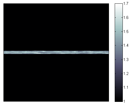
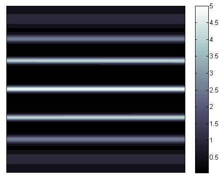
The initial condition (6.1) and the reference solution at final time TfT_{f} are plotted in Fig. 1. The presented figure demonstrates the ability of the model (1.2)–(1.3) to generate stripe patterns. Three-dimensional plots of the cell density using both studied schemes at final time with Δ​t=10−2\Delta t=10^{-2} are presented in Fig. 2. Finally, in Fig. 3, we plot the contour along the line L={0}×(−35,35)L=\{0\}\times(-35,35) of the reference solution and of the solutions computed using both schemes with Δ​t=1\Delta t=1. We can see from this figure that even for a large time-step size, the corrected decoupled scheme is in close agreement with the reference solution, which is not the case of the scheme (2.5)–(2.6).
Refer to caption
Refer to caption
Figure 1: Initial cell density (6.1) (left) and cell density (u)(u) at final time TfT_{f} computed via the corrected decoupled scheme (2.5),(2.12) with Δ​t=10−2\Delta t=10^{-2} (right).
Refer to caption
Refer to caption
Figure 2: Three-dimensional plot of the cell density (u)(u) at final time TfT_{f} computed via the corrected decoupled scheme (2.5),(2.12) (left) and the decoupled scheme (2.5)–(2.6) (right) with Δ​t=10−2\Delta t=10^{-2}.
Refer to caption
Figure 3: Contours along the line LL of the solution (u)(u) at final time TfT_{f}; solid line reference solution, ∘\circ solution computed via the corrected decoupled scheme (2.5),(2.12) with Δ​t=1\Delta t=1, ∗* solution computed via the decoupled scheme (2.5)–(2.6) with Δ​t=1\Delta t=1.

Test 2. The purpose of this test is to investigate the efficiency of the corrected decoupled scheme in the case of the parabolic-parabolic version of the model (1.2)–(1.3).

We consider the same data used in the previous test. Nevertheless, we need to define an initial condition for the concentration of chemoattractant, we take then c⁡(x,0)=1/32c(x,0)=1/32. The schemes adopted are similar to those of the previous test, we only need to replace the equation (2.6) in the scheme (2.5)–(2.6) by

m​(K)​cKn+1−cKnΔ​t−∑σ∈ℰKτσ​D​cK,σn+1+m​(K)​cKn+1=m​(K)​uKnuKn+1,\text{\rm m}(K)\frac{c^{n+1}_{K}-c^{n}_{K}}{\Delta t}-\sum_{\sigma\in\mathcal{E}_{K}}\tau_{\sigma}\,Dc^{n+1}_{K,\sigma}+\text{\rm m}(K)\,c_{K}^{n+1}=\text{\rm m}(K)\,\frac{u_{K}^{n}}{u_{K}^{n}+1}, (6.2)

and we substitute the equation (2.12) in the scheme (2.5),(2.12) by (we recall that βn=1\beta_{n}=1)

m​(K)​cKn+1−cKnΔ​t−∑σ∈ℰKτσ​D​cK,σn+1+m​(K)​cKn+1=m​(K)​uKnuKn+1+TKn.\text{\rm m}(K)\frac{c^{n+1}_{K}-c^{n}_{K}}{\Delta t}-\sum_{\sigma\in\mathcal{E}_{K}}\tau_{\sigma}\,Dc^{n+1}_{K,\sigma}+\text{\rm m}(K)\,c_{K}^{n+1}=\text{\rm m}(K)\,\frac{u_{K}^{n}}{u_{K}^{n}+1}+T_{K}^{n}. (6.3)

The following decoupled scheme is also investigated in this test:

m​(K)​uKn+1−uKnΔ​t−μ​∑σ∈ℰKτσ​D​uK,σn+1\displaystyle\text{\rm m}(K)\frac{u^{n+1}_{K}-u^{n}_{K}}{\Delta t}-\mu\sum_{\sigma\in\mathcal{E}_{K}}\tau_{\sigma}Du_{K,\sigma}^{n+1}
+a∑σ∈ℰKσ=K|Lτσ(S(DcK,σn)uKn+1−S(−DcK,σn)uLn+1)=0,\displaystyle+a\sum_{\begin{subarray}{c}\sigma\in\mathcal{E}_{K}\\ \sigma=K|L\end{subarray}}\tau_{\sigma}\left(S\left(Dc_{K,\sigma}^{n}\right)u_{K}^{n+1}-S\left(-Dc_{K,\sigma}^{n}\right)u_{L}^{n+1}\right)=0, (6.4)
m​(K)​cKn+1−cKnΔ​t−∑σ∈ℰKτσ​D​cK,σn+1+m​(K)​cKn+1=m​(K)​uKn+1uKn+1+1,\displaystyle\text{\rm m}(K)\frac{c^{n+1}_{K}-c^{n}_{K}}{\Delta t}-\sum_{\sigma\in\mathcal{E}_{K}}\tau_{\sigma}\,Dc^{n+1}_{K,\sigma}+\text{\rm m}(K)\,c_{K}^{n+1}=\text{\rm m}(K)\,\frac{u_{K}^{n+1}}{u_{K}^{n+1}+1}, (6.5)

such scheme is used for example in [14].

The reference solution is computed similarly to the previous test. We observe from Table 2 that the scheme (6.4)–(6.5) is the less accurate one. We can see also that the corrected decoupled scheme (2.5),(6.3) is about four to five times more accurate than the scheme (2.5),(6.2).

Δ​t\Delta t L2L^{2}-error Rate L2L^{2}-error Rate L2L^{2}-error Rate
coorected decoupled (2.5),(6.2) (6.4)–(6.5)
55 8.450×10−28.450\times 10^{-2} — 3.775×10−13.775\times 10^{-1} — 4.231×10−14.231\times 10^{-1} —
11 2.323×10−22.323\times 10^{-2} 0.8020.802 1.117×10−11.117\times 10^{-1} 0.7560.756 1.243×10−11.243\times 10^{-1} 0.7610.761
5.10−15.10^{-1} 1.344×10−21.344\times 10^{-2} 0.7900.790 6.109×10−26.109\times 10^{-2} 0.8710.871 6.846×10−26.846\times 10^{-2} 0.8610.861
10−110^{-1} 2.971×10−32.971\times 10^{-3} 0.9380.938 1.314×10−21.314\times 10^{-2} 0.9550.955 1.477×10−21.477\times 10^{-2} 0.9530.953
5.10−25.10^{-2} 1.490×10−31.490\times 10^{-3} 0.9960.996 6.634×10−36.634\times 10^{-3} 0.9860.986 7.456×10−37.456\times 10^{-3} 0.9860.986
10−210^{-2} 2.765×10−42.765\times 10^{-4} 1.051.05 1.354×10−31.354\times 10^{-3} 0.9870.987 1.519×10−31.519\times 10^{-3} 0.9880.988
Table 2: Relative L2L^{2}-errors and time convergence orders obtained for (u)(u) using the corrected decoupled scheme (2.5),(6.3), the decoupled scheme (2.5),(6.2), and the decoupled scheme (6.4)–(6.5).

In Fig. 4, we show the evolution of the cell density by plotting the contour of the reference solution along the line L={0}×(−35,35)L=\{0\}\times(-35,35) at different times.

Refer to caption
Refer to caption
Refer to caption
Refer to caption
Figure 4: Contours along the line LL of the reference solution (u)(u) at t=25t=25 (left top), t=75t=75 (right top), t=100t=100 (left bottom), TfT_{f} (right bottom).

Test 3. The purpose of this test is to study the accuracy of our corrected decoupled scheme when the source term in the equation for concentration cc is linear. To this end, we consider the following chemotaxis-growth model for bacterial pattern formation [1]:

{∂tu=μΔu−χ∇⋅(u∇c)+f(u)inΩ×(0,Tf),∂tc=Δ​c−γ​c+uin​Ω×(0,Tf),\left\{\begin{aligned} &\partial_{t}u=\mu\Delta u-\chi\nabla\cdot(\,u\nabla c)+f(u)\quad\text{in}\ \Omega\times(0,T_{f}),\\ &\partial_{t}c=\Delta c-\gamma c+u\quad\text{in}\ \Omega\times(0,T_{f}),\end{aligned}\right. (6.6)

endowed with the homogeneous Neumann boundary conditions. We consider the following data: μ=0.0625\mu=0.0625, χ=6\chi=6, γ=16\gamma=16, f⁡(u)=2​u​(1−u)f(u)=2u(1-u) and Tf=30T_{f}=30. The computational domain is the square Ω=(−8,8)2\Omega=(-8,8)^{2} discretized with a uniform mesh grid 100×100100\times 100. For all x∈Ωx\in\Omega, we choose the following initial conditions:

u⁡(x,0)={1+ϵ⁡(x)if ​‖x‖2<0.7,1otherwise,u(x,0)=\left\{\begin{array}[]{ll}1+\epsilon(x)&\quad\mbox{if }\|x\|_{2}<0.7,\\ 1&\quad\mbox{otherwise},\end{array}\right.\\

and c⁡(x,0)=1/32c(x,0)=1/32. The random perturbation ϵ⁡(x)\epsilon(x) is defined as in (6.1).

In this test, we compare the numerical results obtained from the decoupled scheme:

m​(K)​uKn+1−uKnΔ​t−μ​∑σ∈ℰKτσ​D​uK,σn+1\displaystyle\text{\rm m}(K)\frac{u^{n+1}_{K}-u^{n}_{K}}{\Delta t}-\mu\sum_{\sigma\in\mathcal{E}_{K}}\tau_{\sigma}Du_{K,\sigma}^{n+1}
+χ∑σ∈ℰKσ=K|Lτσ(S(DcK,σn+1)uKn+1−S(−DcK,σn+1)uLn+1)−2m(K)uKn(1−uKn+1)=0,\displaystyle+\chi\sum_{\begin{subarray}{c}\sigma\in\mathcal{E}_{K}\\ \sigma=K|L\end{subarray}}\tau_{\sigma}\left(S\left(Dc_{K,\sigma}^{n+1}\right)u_{K}^{n+1}-S\left(-Dc_{K,\sigma}^{n+1}\right)u_{L}^{n+1}\right)-2\text{\rm m}(K)\,u_{K}^{n}\left(1-u_{K}^{n+1}\right)=0, (6.7)
m​(K)​cKn+1−cKnΔ​t−∑σ∈ℰKτσ​D​cK,σn+1+γ​m​(K)​cKn+1=m​(K)​uKn,\displaystyle\text{\rm m}(K)\frac{c^{n+1}_{K}-c^{n}_{K}}{\Delta t}-\sum_{\sigma\in\mathcal{E}_{K}}\tau_{\sigma}\,Dc^{n+1}_{K,\sigma}+\gamma\text{\rm m}(K)\,c_{K}^{n+1}=\text{\rm m}(K)\,u_{K}^{n}, (6.8)

with those of the corrected decoupled scheme, consisting of (6.7) and the following equation

m​(K)​cKn+1−cKnΔ​t−∑σ∈ℰKτσ​D​cK,σn+1+γ​m​(K)​cKn+1=m​(K)​uKn+TKn.\text{\rm m}(K)\frac{c^{n+1}_{K}-c^{n}_{K}}{\Delta t}-\sum_{\sigma\in\mathcal{E}_{K}}\tau_{\sigma}\,Dc^{n+1}_{K,\sigma}+\gamma\text{\rm m}(K)\,c_{K}^{n+1}=\text{\rm m}(K)\,u_{K}^{n}+T_{K}^{n}. (6.9)

where for all K∈𝒯K\in\mathcal{T} and n=1,…,N−1n=1,...,N-1

TKn=m​(K)​(uKn−uKn−1),TK0=0.T_{K}^{n}=\text{\rm m}(K)\left(u_{K}^{n}-u_{K}^{n-1}\right),\quad T_{K}^{0}=0.

The reference solution is computed by the corrected decoupled scheme using a very fine time-step size Δ​t=10−4\Delta t=10^{-4}. The results presented in Table 3 show that the corrected decoupled scheme is highly accurate compared to the scheme (6.7)–(6.8). In the case when Δ​t=10−3\Delta t=10^{-3}, the corrected decoupled scheme is about 3232 times more accurate than the scheme (6.7)–(6.8).

Δ​t\Delta t L2L^{2}-error Rate L2L^{2}-error Rate
coorected decoupled decoupled
5.10−15.10^{-1} 4.216×10−34.216\times 10^{-3} — 2.234×10−22.234\times 10^{-2} —
10−310^{-3} 6.022×10−46.022\times 10^{-4} 1.211.21 1.119×10−21.119\times 10^{-2} 0.4300.430
5.10−25.10^{-2} 2.947×10−42.947\times 10^{-4} 1.031.03 6.806×10−36.806\times 10^{-3} 0.7170.717
10−210^{-2} 5.863×10−55.863\times 10^{-5} 1.001.00 1.636×10−31.636\times 10^{-3} 0.8860.886
5.10−35.10^{-3} 2.907×10−52.907\times 10^{-5} 1.011.01 8.385×10−48.385\times 10^{-4} 0.9640.964
10−310^{-3} 5.347×10−65.347\times 10^{-6} 1.051.05 1.707×10−41.707\times 10^{-4} 0.9890.989
Table 3: Relative L2L^{2}-errors and time convergence orders obtained for (u)(u) using the corrected decoupled scheme (6.7),(6.9) and the decoupled scheme (6.7)–(6.8).

The numerical cell density uu of the model computed using both schemes with Δ​t=10−3\Delta t=10^{-3} is shown in Fig. 5. As we can see, the solution forms periodic arrays of continuous rings which match well with the patterns formed by Salmonella typhimurium [21].

Refer to caption
Refer to caption
Figure 5: Cell density (u)(u) at final time TfT_{f} computed via the corrected decoupled scheme (6.7),(6.9) (left) and the decoupled scheme (6.7)–(6.8) (right) with Δ​t=10−3\Delta t=10^{-3}.

Test 4. In this test, we present some numerical simulations which illustrate the ability of the presented corrected decoupled finite volume scheme to capture different forms of bacterial spatial patters. For this purpose, we consider the chemotaxis model (6.6) with the following data used in [1] : μ=0.0625\mu=0.0625, γ=32\gamma=32 and f⁡(u)=u2​(1−u)f(u)=u^{2}\left(1-u\right). The domain is the square Ω=(−10,10)2\Omega=(-10,10)^{2}, which is discretized via a uniform mesh grid 150×150150\times 150, and the time-step used is Δ​t=10−1\Delta t=10^{-1}. For the final time, we take Tf=150T_{f}=150 and we consider the following initial conditions

u⁡(x,0)={1+ϵ⁡(x)if ​‖x‖2<1,1otherwise,u(x,0)=\left\{\begin{array}[]{ll}1+\epsilon(x)&\quad\mbox{if }\|x\|_{2}<1,\\ 1&\quad\mbox{otherwise},\end{array}\right.\\

and c⁡(x,0)=1/32c(x,0)=1/32.

The corrected decoupled scheme used is similar to that of the previous section. However, since the logistic source f⁡(u)f(u) has now a cubic form, we use the following linearized finite volume discretization:

∫Ku​(x,t)2​(1−u⁡(x,t))​𝑑x≈m​(K)​uKn+1​uKn​(1−uKn).\displaystyle\int_{K}u(x,t)^{2}\left(1-u(x,t)\right)\,dx\approx\text{\rm m}(K)\,u_{K}^{n+1}u_{K}^{n}\left(1-u_{K}^{n}\right).

For χ=80\chi=80, the computed solution at t=30t=30 is shown in Fig. 6. We observe from Fig. 6 (left) the formation of symmetrical spots in whole domain. The 3D view of this patterning is presented in Fig. 6 (right).

Refer to caption
Refer to caption
Figure 6: Cell density (u)(u) for χ=80\chi=80 at t=30t=30 computed via the corrected decoupled.

In Fig. 7, we examine the effect of the parameter χ\chi on the numerical solution. When χ=6\chi=6, a honeycomb pattern is observed. Then, the solution changes its structure to continuous rings for χ=7.4\chi=7.4. When χ=20\chi=20, chaotic spots appear. The symmetry of these spots increases for high values of χ\chi (see Fig. 7 (right bottom)). These symmetric spots seem in good agreement with the Escherichia coli patterns reported in [5].

Refer to caption
Refer to caption
Refer to caption
Refer to caption
Figure 7: Cell density (u)(u) computed via the corrected decoupled scheme at final time TfT_{f}, for χ=6\chi=6 (left top), χ=7.4\chi=7.4 (right top), χ=20\chi=20 (left bottom), χ=70\chi=70 (right bottom).

7 Conclusion

In this paper, a decoupled scheme for solving chemotaxis problems is developed. Decoupled schemes are known to be very advantageous in terms of computational cost in comparison to coupled ones, however the major disadvantage of such schemes is their lack of accuracy. The proposed approximation is based on a classical decoupled scheme, which is improved by adding a suitable correction term. This approach does not affect the computational speed of the scheme and is easy to implement. Moreover, the numerical results presented show that our approach is much more accurate than usual decoupled schemes. The question is now to know how we can develop the idea of the scheme to deal with other systems of partial differential equations. This may represent an interesting topic for further research.

References

References

  • [1] Aida, M., Tsujikawa, T., Efendiev, M., Yagi, A., Mimura, M.: Lower estimate of the attractor dimension for a chemotaxis growth system. J. London Math. Soc. 74(2), 453–474 (2006)
  • [2] Akhmouch, M., Benzakour Amine, M.: Semi-implicit finite volume schemes for a chemotaxis-growth model. Indag. Math. 27(3), 702–720 (2016)
  • [3] Akhmouch, M., Benzakour Amine, M.: A time semi-exponentially fitted scheme for chemotaxis-growth models. Calcolo (2016). doi:10.1007/s10092-016-0201-4
  • [4] Andreianov, B., Bendahmane, M., Saad, M.: Finite volume methods for degenerate chemotaxis model. J. Comput. Appl. Math. 235 (14), 4015–4031 (2011)
  • [5] Budrene, E.O., Berg, H.C.: Dynamics of formation of symmetrical patterns by chemotactic bacteria. Nature 376, 49–53 (1995)
  • [6] Chainais-Hillairet, C., Liu, J.-G., Peng, Y.-J: Finite volume scheme for multi-dimensional drift-diffusion equations and convergence analysis. Math. Mod. Numer. Anal. 37, 319–338 (2003)
  • [7] Oster, G.F., Murray, J.D.: Pattern Formation Models and Developmental Constraints. J. expl. Zool. 251, 186-202 (1989)
  • [8] Keller, E.F., Segel, L.A.: Travelling bands of chemotactic bacteria: a theoretical analysis. J. Theor. Biol. 30, 235-248 (1971)
  • [9] Murray, J.D., Deeming, D.C., Ferguson, M.W.J.: Size dependent pigmentation pattern formation in embryos of Alligator mississippiensis: time of initiation of pattern generation mechanism. Proc. R. Soc. B 239, 279-293 (1990)
  • [10] Myerscough, M.R., Murray, J.D.: Analysis of propagating pattern in a chemotaxis system. Bull. math. Biol. 54, 77-94 (1992)
  • [11] Patankar, S.V.: Numerical Heat Transfer and Fluid Flow, Hemisphere Publishing Corporation, Taylor and Francis Group, New York (1990)
  • [12] Saito, N.: Conservative upwind finite-element method for a simplified Keller-Segel system modelling chemotaxis, IMA J. Numer. Anal. 27, 332-365 (2007)
  • [13] Saito, N., Suzuki, T.: Notes on finite difference schemes to a parabolic-elliptic system modelling chemotaxis. Appl. Math. Comput. 171(1), 72–90 (2005)
  • [14] Strehl, R., Sokolov, A., Kuzmin, D., Turek, S.: A flux-corrected finite element method for chemotaxis problems. Comput. Methods Appl. Math. 10(2), 219–232 (2010)
  • [15] Filbet, F.: A finite volume scheme for the Patlak-Keller-Segel chemotaxis model, Numer. Math. 104(4), 457-488 (2006)
  • [16] Chamoun, G., Saad, M., Talhouk, R.: Monotone combined edge finite volume-finite element scheme for anisotropic Keller-Segel model. Numer. Methods Partial Differential Equations 30 (3), 1030-1065 (2014)
  • [17] Ibrahim, M., Saad, M.: On the efficacy of a control volume finite element method for the capture of patterns for a volume-filling chemotaxis model. Comp. Math. Appl. 68, 1032–1051 (2014)
  • [18] Eymard, R., Gallouët, T., Herbin, R.: Finite volume methods. In: P. G. Ciarlet and J. L. Lions(eds.), Handbook of numerical analysis volume VII, 713-1020, North-Holland (2000)
  • [19] Bessemoulin-Chatard, M., Chainais-Hillairet, C., Filbet, F.: On discrete functional inequalities for some finite volume schemes. IMA J. Numer. Anal. 35(3), 1125–1149 (2015)
  • [20] Spalding, D.B.: A novel finite difference formulation for differential expressions involving both first and second derivatives. Int. J. Numer. Methods Eng. 4, 551–559 (1972)
  • [21] Woodward D., Tyson R., Myerscough M., Murray J., Budrene E., Berg H.: Spatio-temporal patterns generated by S. typhimurium. Biophys. J. 68, 2181–2189 (1995)