Megaparsec-scale structure around the proto-cluster core SPT234956 at 2020Megaparsec-scale structure around the proto-cluster core SPT234956 at –
Abstract
We present an extensive ALMA spectroscopic follow-up programme of the structure SPT234956, one of the most actively star-forming proto-cluster cores known, to identify additional members using their [Cii] 158 m and CO(4–3) lines. In addition to robustly detecting the 14 previously published galaxies in this structure, we identify a further 15 associated galaxies at , resolving 555 per cent of the 870-m flux density at 0.5 arcsec resolution compared to 21 arcsec single-dish data. These galaxies are distributed into a central core containing 23 galaxies extending out to 300 kpc in diameter, and a northern extension, offset from the core by 400 kpc, containing three galaxies. We discovered three additional galaxies in a red Herschel-SPIRE source 1.5 Mpc from the main structure, suggesting the existence of many other sources at the same redshift as SPT234956 that are not yet detected in the limited coverage of our data. An analysis of the velocity distribution of the central galaxies indicates that this region may be virialized with a mass of (95)1012 M⊙, while the two offset galaxy groups are about 30 and 60 per cent less massive and show significant velocity offsets from the central group. We calculate the [Cii] and far-infrared number counts, and find evidence for a break in the [Cii] luminosity function. We estimate the average SFR density within the region of SPT234956 containing single-dish emission (a proper diametre of 720 kpc), assuming spherical symmetry, to be roughly 4 M⊙ yr-1 Mpc-3; this may be an order of magnitude greater than the most extreme examples seen in simulations.
Keywords:
galaxies – formation: galaxies – evolution: submm – galaxies1 Introduction
The largest gravitationally-bound objects in the Universe are galaxy clusters, which have evolved from the largest overdensities seeded in the very early Universe into Mpc-sized structures presently containing thousands of galaxies. Cosmological simulations and observations indicate that these structures are built up hierarchically, where small overdensities initially collapsed and later merged to form large overdensities; however, the details of this process are far from understood, and in particular, we don’t yet know how cluster formation affects galaxy evolution, and what roles may be played by active galactic nuclei (AGN) feedback (McNamara & Nulsen 2012; Pike et al. 2014; Smolčić et al. 2017, e.g.,), or by star-formation downsizing (Magliocchetti et al. 2013; Miller et al. 2015; Wilkinson et al. 2017, e.g.,).
One way to investigate these issues is to look for clues in local, fully-formed clusters. Local clusters are dominated by elliptical galaxies (Dressler 1980, e.g.) that are much more red than their field counterparts (Wake et al. 2005; Stott et al. 2007, e.g.,), and similarly show very little star-formation activity (Balogh et al. 1998; Lewis et al. 2002; Tanaka et al. 2004, e.g.,). These observations suggest that the bulk of the star-formation activity in galaxy clusters occurred before redshifts of 2 (Snyder et al. 2012; Willis et al. 2020, e.g.,).
A more direct way to investigate galaxy cluster formation is to observe galaxy clusters at high redshifts. We now find galaxy clusters out to redshift 2 by looking for observational signatures such as X-rays emitted by hot inter-cluster gas (Rosati et al. 2009; Gobat et al. 2011; Andreon et al. 2014; Wang et al. 2016; Mantz et al. 2018, e.g.,), the Sunyaev-Zeldovich effect (Planck Collaboration XXVII 2016; Bleem et al. 2015; Huang et al. 2020, e.g.,), and galaxy-based searches (Andreon & Huertas-Company 2012; Papovich et al. 2010; Zeimann et al. 2012; Stanford et al. 2012; Muzzin et al. 2013, e.g.,). However, beyond this epoch, these observational signatures become much less defined as these structures have not yet virialized. With this in mind, following Overzier 2016, we adopt the definition that a ‘galaxy cluster’ is a virialized object with M⊙, and a ‘proto-cluster’ is a structure that will one day become a galaxy cluster. Proto-clusters may have high merger rates and correspondingly high star-formation rates (Casey 2016, SFRs; e.g.), thus containing a large number of dusty galaxies. These galaxies would then be more easily observed as luminous starbursts at millimetre/submillimetre (mm/submm) wavelengths and as AGN at radio wavelengths (Miley & De Breuck 2008; Galametz et al. 2013; Rigby et al. 2014, e.g.,), motivating searches in these regimes.
Distant proto-clusters are excellent laboratories for studying not only the details of cluster formation, but also galaxy evolution and star formation, since these processes are likely undergoing their most active phase at this epoch. A number of proto-clusters have been discovered beyond redshifts of 2, typically through their rest-frame optical emission, which traces unobscured stellar light (Steidel et al. 2000; Shimasaku et al. 2003; Steidel et al. 2005; Venemans et al. 2007; Chiang et al. 2015; Dey et al. 2016; Harikane et al. 2019, e.g.,), or as overdensities of submm galaxies (SMGs), which probes their rest-frame far-infrared emission and traces star formation (Tamura et al. 2009; Chapman et al. 2009; Dannerbauer et al. 2014; Chiang et al. 2015; Flores-Cacho et al. 2016; Umehata et al. 2015; Casey et al. 2015; Hung et al. 2016; Oteo et al. 2018; Lacaille et al. 2019; Kneissl et al. 2019, e.g.,). However, comparing these systems to current simulations is challenging due to their very low number density, which requires large simulated cosmological volumes, and because they contain very massive galaxies with high gas and stellar densities that require significant resolution to simulate accurately.
Recently, one such structure, SPT234956, was identified as an incredibly luminous 870-m flux density source at redshift 4.3 (mJy, corresponding to a SFR 104 Myr-1) within which 14 SMGs were spectroscopically confirmed in the core region, making it potentially one of the highest density proto-clusters known at this epoch (Miller et al. 2018). However, only the central component of the structure was probed, and 36 per cent of the single-dish flux density resolved, leaving open the possibility that the remaining flux density could be due to chance alignments along the line of sight (Hayward et al. 2018, e.g.,). Establishing more proto-cluster members through further spectroscopic observations would provide further evidence that this system is the progenitor to a rich galaxy cluster (perhaps even as large as the Coma Cluster), as opposed to a starved core that evolves into a much smaller galaxy group (as seen in some systems, see e.g. Lovell et al. 2018). Additionally, redshift 4.3 SMGs in the field are known to be quite rare (Chapman et al. 2005; Simpson et al. 2014, the median redshift being about 2.5, see), making this a particularly interesting and statistically robust sample of galaxies undergoing accelerated evolution from which we can learn about the complex interplay between star formation, galaxy formation, and cluster formation.
In this paper, we report the results from an extensive follow-up programme of SPT234956 using the Atacama Large Millimeter/submillimeter Array (Wootten & Thompson 2009, ALMA;), which aimed to spectroscopically confirm new proto-cluster members and spatially resolve the galaxies responsible for the intense star-formation observed. In Section 2, we outline how SPT234956 was selected, summarize previous observations of this proto-cluster, and describe our new ALMA follow-up efforts. In Section 3 we present our data analysis methods, including our search for new galaxies, and in Section 4 we present our results. Section 5 discusses our findings, and the paper is summarized and concluded in Section 6 . We assume a CDM model with parameters from Planck Collaboration XIII 2016 throughout.
2 Observations
2.1 Selection from the South Pole Telescope survey
SPT234956 was initially discovered as part of the South Pole Telescope (SPT) extragalactic mm-wave point-source catalogue (Vieira et al. 2010; Mocanu et al. 2013; Everett et al. 2020), a collection of bright (mJy at ) sources found in the SPT 2500 deg2 survey that are unresolved by SPT’s 1 arcmin beam. From a total sample of over 1000 objects, roughly 200 were classified as dusty star-forming galaxies based on their spectral indices. Of these, the brightest were followed up with the Atacama Pathfinder Experiment (APEX) telescope’s Large APEX BOlometer CAmera (Kreysa et al. 2003; Siringo et al. 2009, LABOCA;) instrument at 870 m, and a flux selection was made at mJy, resulting in a final sample of 81 SMGs.
A dedicated follow-up campaign using a number of optical-through-mm wavelength facilities, including ALMA, the Spectral and Photometric Imaging REceiver (Griffin et al. 2010, SPIRE;) on board the Herschel satellite, and Spitzer’s Infrared Array Camera (Fazio et al. 2004, IRAC;), was subsequently undertaken to determine the nature of these incredibly bright star-forming galaxies (Vieira et al. 2013; Weiß et al. 2013); some reached flux densities of 100 mJy at 870 m, meaning that they could only be strong gravitational lenses or collections of galaxies densely packed within SPT’s 1 arcmin beam. It was found that about 90 per cent of the sources are indeed strong gravitational lenses with magnification factors reaching up to about 30, and that the remaining 10 per cent show no evidence for lensing and are instead likely to be intrinsically ultra-luminous galaxies or collections of galaxies (Hezaveh et al. 2013; Spilker et al. 2016).
SPT234956 is the brightest of these unlensed sources, with mJy. Further follow-up with ALMA in Cycle 1 at 3 mm and with the APEX telescope’s First Light APEX Submillimeter Heterodyne (Heyminck et al. 2006, FLASH;) instrument revealed that the structure is composed of a bright central component at a redshift of 4.3 (Greve et al. 2012; Strandet et al. 2016), and a fainter northern extension (see Fig. 1).
2.2 Follow-up ALMA observations
Since its discovery and redshift determination, SPT234956 has been the subject of numerous ALMA follow-up studies. High-resolution spectroscopy targeting the CO(4–3), [Cii] 158 m, and [Nii] 205 m transitions in the core region of SPT234956 were carried out in Cycles 3 and 4 and used to securely identify 14 central galaxies (Miller et al. 2018); for reference, the depths of these observations were 0.2 mJy beam-1 for the CO(4–3) transition, 1.1 mJy beam-1 for the [Cii] transition, and 0.4 mJy beam-1 for the [Nii] transition. Here we report on a suite of new ALMA observations undertaken during Cycles 5 and 6, covering a much larger area with greater depth.
The Cycle 5 observations used in this paper targeted two of the lines observed in the previous cycles, [Cii] in Band 7 (GHz) and CO(4–3) in Band 3 (GHz). Our [Cii] coverage included a three-pointing mosaic of the brighter central component of SPT234956, covering a much larger area than the existing data, and a single pointing of the previously unobserved northern component, both down to a depth of about 0.3 mJy beam-1 per 13 km s-1 channel. Our CO(4–3) pointings covered the entire 870-m emission region, including the previously unobserved northern component, down to 0.07 mJy beam-1 per 54 km s-1 channel. The [Cii] observations were tuned to place the line in the centre of the upper sideband, while for the CO(4–3) observations the tuning was set to place the line in the lower sideband.
The Cycle 6 observations presented in this paper also targeted the [Cii] and CO(4–3) transitions in Bands 7 and 3, respectively. The goal of the [Cii] observations was to cover most of the central component of SPT234956 with a frequency setup similar to that of the Cycle 5 data, but with higher angular resolution in order to resolve morphologies. The goal of the CO(4–3) observations was to provide coverage of the outskirts of the structure. The setup of these Band 3 observations was also chosen to be similar to that of the Cycle 5 CO(4–3) observations in order to allow the data to be combined into a single deep CO(4–3) map. The depth of the Band 7 data was approximately 0.4 mJy beam-1 per 13 km s-1 channel, and the depth of the Band 3 data was approximately 0.06 mJy beam-1 per 54 km s-1 channel. We note that the Cycle 5 and 6 depths quoted above do not include existing observations from previous cycles.
In addition to targeting the main structure of SPT234956, we also used existing Herschel-SPIRE data to identify five red Herschel sources surrounding SPT234956 using 250 m positions as priors; here ‘red’ is defined as , with a signal-to-noise above 3 at both 250 and 500 m (see Miller et al. 2018 for details). One of these five sources lies close to the central structure and was covered by our extended CO(4–3) mosaic; the remaining four sources were targeted in dedicated Band 3 observations in Cycle 6, with the expected CO(4–3) transition centred in the lower sideband, and these pointings reached depths of 0.1–0.2 mJy beam-1 per 54 km s-1 channel. An overview of the observations is shown in Fig. 1 and summarized in Table 1. It is also important to recall that the sensitivity of these observations to source-detection depend on the synthesized beams, which in turn depend on the array configurations – thus in Table 1 we also provide beamsizes for each dataset.

| Cycle | Description | Line transition | Channel width | RMS per channel | Synthesized beamsize | Area |
| [km s-1] | [mJy beam-1] | major/minor [arcsec] | [arcmin2] | |||
| 5 | 3-point mosaic of central LABOCA source | [Cii] | 13 | 0.27 | 0.56/0.49 | 0.33 |
| 5 | Single pointing of northern LABOCA source | [Cii] | 13 | 0.32 | 0.51/0.38 | 0.13 |
| 5 | 2-point mosaic of entire LABOCA source | CO(4–3) | 54 | 0.072 | 1.01/0.84 | 2.8 |
| 6 | 6-point mosaic of central LABOCA source | [Cii] | 13 | 0.41 | 0.23/0.17 | 0.45 |
| 6 | 8-point mosaic of outer LABOCA region | CO(4–3) | 54 | 0.14 | 0.52/0.45 | 9.2 |
| 6 | Single pointing of SPIREb | CO(4–3) | 54 | 0.13 | 1.03/0.81 | 1.9 |
| 6 | Single pointing of SPIREc | CO(4–3) | 54 | 0.17 | 0.71/0.61 | 1.7 |
| 6 | Single pointing of SPIREd | CO(4–3) | 54 | 0.12 | 0.97/0.83 | 1.9 |
| 6 | Single pointing of SPIREe | CO(4–3) | 54 | 0.14 | 0.94/0.82 | 1.9 |
| 5+6 | Combined map of central LABOCA sourcea | [Cii] | 13 | 0.22 | 0.35/0.29 | 0.43 |
| 5+6 | Combined map of outer LABOCA regionb | CO(4–3) | 54 | 0.064 | 0.85/0.72 | 7.2 |
- •
aCombination of the 3-point mosaic of the central LABOCA source from Cycle 5 and the 6-point mosaic of the central LABOCA source from Cycle 6.
- •
bCombination of the 2-point mosaic of the entire LABOCA source from Cycle 5 and the 8-point mosaic of the outer LABOCA region from Cycle 6.
3 Data analysis
3.1 Data reduction
The ALMA data were calibrated using casa11 1 https://casa.nrao.edu (McMullin et al. 2007) and the observatory-provided calibration scripts. Dirty and cleaned data cubes for each of the observations reported in Table 1 were produced using the casa function tclean with Briggs weighting and a robust parameter of 0.5. Continuum images were also produced using tclean for the sidebands that did not contain any line emission using multi-frequency synthesis (MFS).
Additionally, we combined the data from the Cycle 5 and 6 observations of [Cii] in the core region (‘3-point mosaic of central LABOCA source’ and ‘6-point mosaic of central LABOCA source’ in Table 1) to produce a single, deep [Cii] data cube, and similarly we combined the tables from the Cycle 5 and 6 observations of CO(4–3) around the entire structure (‘2-point mosaic of entire LABOCA source’ and ‘8-point mosaic of outer LABOCA region’ in Table 1) to produce a deep data cube of CO(4–3). The maximum depth of the deep [Cii] map was 0.2 mJy beam-1 per 13 km s-1 channel, and the synthesized beam major/minor full width at half maximum (FWHM) was 0.35/0.29 arcsec. For the deep CO(4–3) map, the maximum depth achieved was 0.06 mJy beam-1 per 54 km s-1 channel and the synthesized beam major/minor FWHM was 0.85/0.72 arcsec.
3.2 Source extraction
Given the significantly deeper data for the core of SPT234956 compared to that reported in Miller et al. 2018 (which was 0.9 mJy beam-1 per 13 km s-1 channel at the observed [Cii] frequency), we expect to discover a number of new sources in both line emission and in the continuum. However, lacking any knowledge of where these new sources might be in our data cubes, it was necessary to perform a source search over the entire surveyed area around the frequencies of the expected lines. In addition, since some of the fainter sources in Miller et al. 2018 were not significantly detected in [Cii] but instead were derived from a joint analysis of [Cii] and CO(4–3), we would like to confirm their [Cii] properties.
To accomplish this, we used the publicly-available code LineSeeker (see González-López et al. 2017; González-López et al. 2019, for details). Briefly, LineSeeker convolves a primary beam-uncorrected data cube with a number of Gaussians of varying width along the spectral axis. The noise per channel is assessed iteratively by computing the standard deviation of all the pixels in a given channel, then re-computing the standard deviation of all the pixels whose absolute values are lower than 5 times the initial noise estimate. Signal-to-noise ratio (S/N) peaks are then located in both positive and negative flux density pixels and returned to the user.
We ran LineSeeker on a total of seven data cubes: 1) the combined, extra-deep [Cii] map of the main core region; 2) the combined, deep CO(4–3) map of the entire structure plus the outskirts; 3) the [Cii] map of the fainter northern region; and 4–7) the four pointings of surrounding red Herschel sources. Here we chose to search for sources through the dirty data cubes in order to minimize the possibility of picking up artefacts introduced by the cleaning. We searched for [Cii] peaks ranging from a single channel to 1000 km s-1 in FWHM, over a velocity range encompassing 1500 km s-1 relative to the mean redshift of 4.304 reported by Miller et al. 2018. This velocity range corresponds to the total bandwidth available in the sideband containing the expected [Cii] emission. Within each data cube we took all positive-pixel line peaks with a S/N greater than the most significant negative-pixel line peak to be detections.
In the [Cii] map of the core, we found negative peaks down to a S/N of 6.2. Using this as our threshold, we identified the 14 known sources found by Miller et al. 2018, and nine new sources. In the [Cii] pointing of the northern region there were negative peaks down to a S/N of 5.9, but only one bright source was found to be more significant than this. Across our deep CO(4–3) map the most significant negative peak was at a S/N of 5.9, and in addition to finding 11 of the above [Cii] sources, two additional sources were found just outside of our [Cii] coverage in the northern region. Out of our four red Herschel targets, sources were only found in one pointing, SPIREc. Here, the most negative peak was at a S/N of 5.6, and three sources were more significant than this. In the other three pointings, SPIREb, SPIREd, and SPIREe, negative peaks were seen down to 5.9, 6.1, and 6.3, respectively. There were no correspondingly more significant positive peaks. Despite the fact that these Herschel follow-up pointings did not turn up any sources, we note that the targets were all quite low S/N in the SPIRE data, and none showed significant 870-m emission in our LABOCA map. This means that there could be other red sources at the same redshift as SPT234956 with low S/N in the Herschel data that we have not yet targeted.
We also searched our maps for continuum sources (i.e. interloping foreground/background sources not associated with the structure of SPT234956) by averaging over all channels. The noise levels of these continuum maps were estimated on a pixel-by-pixel basis by calculating the local rms within circles of 6 arcsec (after masking all of the sources detected by their line emission), and then we ran a peak-finding algorithm on the resulting maps, looking for both positive flux density and negative flux density peaks. Similar to our line search, we looked for positive flux density peaks with a higher significance than the most significant negative flux density peak. This time we chose one S/N cutoff for all Band 3 data and another for all Band 7 data, based on the most significant negative peaks across all five and two maps, respectively.
This continuum search found negative peaks down to a S/N of 5.0 in the Band 3 data and 5.6 in the Band 7 data. While no new sources were found in the Band 3 data that are more significant than a S/N of 5.0, two were found in the Band 7 data in the central region and one in the northern region. These 29 line detections and three continuum detections constitute our current sample of SPT234956 galaxies, and are summarized in Fig. 2. Sources are named firstly according to the region where they are located, where ‘C’ refers to the core, ‘N’ refers to the northern component, and ‘SPIREc’ refers to the red Herschel source SPIREc, and secondly in order of decreasing [Cii] line strength for the core, and decreasing CO(4–3) line strength for the northern component and SPIREc (see Section 3.4 for details about line strength measurements). Continuum-only sources are designated as ‘NL’ (no line) and ordered by decreasing 850 m flux density.
3.3 Extended [Cii] emission
Around the bright central galaxies C3, C6, and C13 (see Fig. 2) an arc of extended [Cii] gas is seen between 357.98 and 358.33 GHz, or between 130 and 420 km s-1 relative to the mean redshift of the structure. The typical specific intensity of this arc is about 1 mJy arcsec-2 at a single channel, with peaks at the 2 mJy arcsec-2 level, and the local noise was estimated to be 0.3 mJy arcsec-2 by taking the rms within a 6 arcsec-diametre circular aperture just outside of the extended emission region after masking all known sources. The diametre of this arc is roughly 2.8 arcsec, or about 19 kpc in proper distance. To investigate this extended emission, we average over these frequencies (i.e. compute a moment 0 map) while masking pixels below 1 and above 10 (where is the local rms, calculated in the same way as above). The resulting map is shown as the inset in Fig. 2, along with 1.25-level contours. It can be seen that there is extended emission above the 1.25 level encircling a number of central galaxies, and in particular sources C16, C22, and C23 are embedded within it (source C11 is spatially close to this emission as well, but has a significantly different velocity offset). We note that there is no clear sign of this extended gas in the CO(4–3) data.
There are many ways to explain the nature of the extended emission seen here, including tidal tails resulting from gravitational interactions amongst galaxies, in particular through major mergers (Toomre & Toomre 1972; Barnes 1988, e.g.,), or an expanding shell of ionized gas (as seen for example in local gas-rich galaxies, e.g., Heiles 1979; McClure-Griffiths et al. 2002). Extended gas emission has been detected in some proto-clusters through the CO(1–0) transition (Emonts et al. 2016; Dannerbauer et al. 2017), the CO(3–4) transition (Ginolfi et al. 2017), and in [Ci] (Emonts et al. 2018), and it has also been statistically detected surrounding 4–7 galaxies through stacking analyses (Fujimoto et al. 2019; Ginolfi et al. 2020). The extended gas in these systems could affect the evolution of the embedded galaxies (Dannerbauer et al. 2017, see e.g.), although the number of sources available for such an analysis still remains low. However, a more thorough analysis is required to understand what we are seeing here, and will be done in future work.

3.4 Source properties
The statistical properties of our un-combined maps, where the array was in a single configuration, are more homogenous and easy to estimate (i.e. the depth is more uniform throughout most of the surveyed area), and additionally have lower angular resolution, reducing the amount of resolved-out flux, thus we estimated the continuum strengths and line properties of our sources using the Cycle 5 3-pointing mosaic for the central sources, and the Cycle 5 single-pointing for the northern sources. Similarly, for Band 3 we used the Cycle 5 2-pointing mosaic to measure line and continuum properties. Lastly, the high-resolution Band 7 imaging from Cycle 6 was used to estimate the sizes of our sources. All line and continuum measurements were made on primary beam-corrected maps.
3.4.1 Line and continuum emission
There are many ways to measure line strengths and continuum flux densities of galaxies in inteferometric data. For example, one could model the galaxies directly in the plane; however, some of our data cubes contain over 20 galaxies, many of which are somewhat resolved, as well as extended emission, making such a procedure very computationally expensive. Instead, we choose to obtain these properties through aperture photometry, and then to compare the results to peak flux photometry to assess if our sources are indeed resolved. Elliptical apertures were designed for each source manually using the [Cii] data cubes (or otherwise the CO(4–3) data cubes when no [Cii] imaging was available) as follows.
First, 2 arcsec-diametre circular apertures were placed on each source, and spectra were obtained by integrating over the pixels and binning the channels by a factor of 4 in order to reduce the noise. From the resulting spectra we tried fitting a constant, a single Gaussian and a double Gaussian model to the line profiles, and took the model with the reduced closest to 1 to be the best fit. We then stacked the channels from to (where is the standard deviation of the best-fitting linewidth), or for cases where two Gaussians was a better fit, from to , where and are from the left and right Gaussian fits, respectively. We also stacked the channels that did not contain line emission to produce continuum images. We plotted our apertures overtop of these line and continuum images and adjusted the apertures to enclose each source out to about 2 in the image plane, then repeated the procedure until the apertures enclosed each source in our best-fitting line and continuum stacks out to 2. These same apertures were then used on the CO(4–3) maps, and for our CO(4–3) spectra the noise was reduced by binning by a factor of 2.
For the three galaxies detected only in the continuum (NL1, NL2, and NL3) the best-fitting models are a constant; these sources could be chance line-of-sight alignments of galaxies at other redshifts, or sources with small line/continuum ratios. We note that NL1 and NL3 also lie close to the edge of our [Cii] maps where the primary beam response is low, making it possible that their [Cii] lines are simply undetected due to the noise. These sources might also be outside of the velocity range probed by our [Cii] observations (1500 km s-1) and too faint in CO(4–3); this interpretation is consistent with NL2 and NL3, whose 850 m continuum flux densities are the same magnitude as other sources with no (or low S/N) CO(4–3) detections, but NL1 is much brighter at 850 m, and sources of similar brightness have well-detected CO(4–3) lines.
Redshifts were determined from the best-fitting Gaussian means, and line strengths were obtained by integrating the spectra from to . In the case of a two-peaked fit, we calculated the best-fitting amplitude-weighted average of the two best-fitting means to calculate a redshift, and the integration bound for the line strength was to . Continuum flux densities were measured in the line-free continuum stacks using the same photometry apertures. Positions were calculated from the brightest pixel in the stacked line images except for NL1, NL2, and NL3, where we used the brightest pixel in the stacked continuum images.
We checked that our apertures were not missing flux by comparing line strengths and continuum flux densities computed with larger aperture sizes. We looked at 10 bright and isolated sources, then determined their line strengths by integrating over the same frequency range as above but increasing the aperture size by 1 pixel up to 6 pixels, and similarly determined their continuum flux densities by stacking the remaining line-free channels. We found that over this aperture range half of the resulting line strengths increased by less than 2 per cent relative to the apertures we used for our measurements, and the remaining half increased by less than 15 per cent, while seven continuum flux densities strictly decreased and the remaining three increased by less than 2 per cent. Therefore, while increasing our aperture sizes may capture more line emission, it would also on average result in a loss in continuum flux density, thus our apertures should be striking a good balance between these two measurements.
We also made line strength and continuum flux density measurements assuming that our sources are unresolved. To do this, for each source we took the stacked line emission maps and obtained spectra at the positions of the brightest pixel, then integrated the spectra across the same channels as in our aperture photometry analysis. Similarly, continuum flux densities were obtained from the brightest pixels in the stacked continuum maps. For the 10 brightest isolated sources, we found that the median ratio of peak-pixel to aperture-photometry line strength in the [Cii] cubes was 0.52, and 0.80 for the continuum flux density ratio. These results show that for our higher frequency data, some galaxies are indeed somewhat resolved. For the CO(4–3) data cubes, these ratios are 1.08 and 1.09, respectively, showing that here our data are consistent with point sources, but that we are not missing much flux in our apertures. For the remainder of this work, we use only measurements obtained from aperture photometry.
We found that the weighted mean redshift of the sources located within the core is 4.302800.00002, in agreement with the findings of Miller et al. 2018, who determined the mean redshift of the core sources to be 4.3040.002. Meanwhile, the weighted mean redshift of the northern component is 4.313090.00016 (a velocity offset of 580 km s-1 relative to the core), and that of SPIREc is 4.281710.00018 (a velocity offset of -1200 km s-1 relative to the core). For the remainder of this paper, we report all line-of-sight velocities relative to the mean redshift of the main central component.
In Table 2 we provide the positions, relative velocities, and continuum flux densities of all 32 galaxies in our sample, and for completeness we also give continuum flux densities at 1.1 mm independently derived from the Band 7 imaging described in Miller et al. 2018 using the same method and apertures outlined above. Here, the positions and relative velocities are from our [Cii] detections when possible, but for galaxies N2, N3, SPIREc1, SPIREc2, and SPIREc3, which only have CO(4–3) observations, we report positions and relative velocities measured from the CO(4–3) line. For galaxies NL1, NL2, and NL3, where no line was detected, we provide the positions of the peak pixels in the continuum maps. For cases where the continuum flux density S/N was less than 2 we give 1 upper limits. We note that sources C3 and C12, as well as sources C13 and C16, are completely blended in the CO(4–3) data cubes. Since sources C3 and C13 are much brighter than sources C12 and C16, respectively, we simply report C12 and C16 as non-detections in Band 3 and provide line and continuum measurements of C3 and C13 only.
In Table 3 we give the integrated line strengths, line luminosities, and linewidths obtained from the fits. Where the line profile is best fit by a double Gaussian, we report both FWHM. For cases where no line is detected we provide 1 upper limits on line strengths and luminosities calculated as the average uncertainty from our measurements. Cutouts of all these sources, showing both stacked continuum and line emission contours, alongside their corresponding spectra with best-fitting Gaussian profiles, are shown in in Appendix A.
3.4.2 Far-infrared luminosities
We model the spectral energy distributions (SEDs) of our dusty submm galaxies following the greybody function outlined in Greve et al. 2012:
| (1) |
where is the critical frequency (or wavelength), is the emissivity index of the dust, is the dust temperature, and and are the Planck and Boltzmann constants, respectively. The continuum flux density measurements presented in this paper do not reach the peak of this SED (about 400 m in the observed frame assuming fiducial model parameters), but instead lie in the Rayleigh-Jeans (long wavelength) regime, meaning that we can explore the range of model parameters that are consistent with the colours (i.e. slopes) seen in our data – a more detailed SED analysis using additional mid-infrared photometry will be presented in a future paper.
In Fig. 3 we have plotted the continuum flux density ratio versus for all central sources with a detection in at least one of these wavelengths, and we show upper limits for the non-detections. We see that the sources with available and flux density measurements (11 in total) have similar colours (albeit with some spread), and we calculate the weighted mean flux density ratio to be 70 with a weighted standard deviation of 10. We note that the upper limits provided by sources lacking one of these continuum measurements are also consistent with this mean colour, except for one outlying source, C17, which has strong 3.2 mm emission but is undetected at 850 m.
We next investigate the range of dust temperatures consistent with the observed spread in by fixing the emissivity index to 2, the critical wavelength to 100 m, and adopting the mean cluster redshift of 4.303. We then calculate the colours predicted by Eq. 1 for a range of finely-gridded dust temperatures, and check to see if the colours fall within the observed weighted standard deviation. In Fig. 3 we show our results, finding that consistent dust temperatures range from 35.2 to 44.8 K and that K provides the closest match to the observed weighted mean colour. This is in agreement with results from Strandet et al. 2016, who found the median dust temperature of SPT SMGs to be 39K, and in particular estimated the SPT234956 dust temperature to be 46.72.8 K.
We next fit the amplitude of the greybody SED of Eq. 1 to each source with one or more continuum detections (see Table 2) using the same parameters as above and with K; for sources with one flux density detection, this simply amounts to scaling the greybody function. The best-fitting models were integrated from 42 to 500 m in order to obtain far-infrared luminosities (), consistent with the integration range used in similar studies, and uncertainties were estimated by adding in quadrature the uncertainty from the fit and the difference in the far-infrared luminosity obtained from using the lower and upper limits for (35.2 K and 44.8 K, respectively) found above. For sources with no continuum detections we scale our upper limits (except for source N3, where we scale our upper limit) to obtain upper limits on . We lastly use a conversion factor of 0.95 M⊙ yr-1/L⊙ (from Kennicutt 1998, modified for a Chabrier initial mass function; see Chabrier 2003) to convert the far-infrared luminosities into SFRs; these values are all provided in Table 2.

3.4.3 Half-light radii
Lastly, half-light radii were measured using the high-resolution Band 7 dust continuum data obtained in Cycle 6. As shown in Table 1, the resolution of this data is about 0.2 arcsec, sufficient to resolve many of the galaxies in our sample, but on the other hand the depth is about 25 per cent worse than the Band 7 data covering the same region from Cycle 5, thus we only expect to see resolved images of our brightest sources.
Based on our best-fitting Gaussian frequency profiles described above, we created 33 arcsec cutouts of each source by stacking the frequency channels in our high-resolution data containing no line emission in order to produce high-resolution continuum images. We then modelled these images as elliptical Sérsic profiles convolved with the best-fitting elliptical Gaussian synthesized beam produced by tclean during the imaging process, and we allowed the Sérsic index to vary. Since many sources are not detected in the continuum in this data, fits were only done for sources brighter than 3 in the continuum stacks. We also note that source C7 resolves into a complicated structure, possibly a pair of merging galaxies, and we do not attempt to fit a Sérsic profile and measure a half-light radius for it. The best-fitting half-light radii, which in our model indicates the sizes of the major axes, are provided in Table 2, and in Appendix B we show the high-resolution continuum images, best-fitting models, and residuals. We find that the half-light radii range from 0.7 to 2.1 kpc, with a mean of 1.5 kpc and a dispersion of 0.5 kpc.
| Name | Ra Dec | SFRh | |||||||
|---|---|---|---|---|---|---|---|---|---|
| [J2000] | [km s-1] | [kpc] | [kpc] | [Jy] | [mJy] | [mJy] | [ L⊙] | [M⊙ yr-1] | |
| Core | |||||||||
| C1 (A) | 23:49:42.65 56:38:19.4 | 154 | 2.010.01 | 323 | 1338 | 6.210.22 | 8.410.14 | 1030 | 980 |
| C2 (J) | 23:49:43.25 56:38:30.1 | -5442 | 2.100.06 | 663 | 229 | 1.080.15 | 1.720.10 | 210 | 200 |
| C3 (B) | 23:49:42.78 56:38:23.8 | -8611 | 0.910.02 | 212 | 835 | 5.170.05 | 6.720.07 | 890 | 840 |
| C4 (D) | 23:49:41.41 56:38:22.5 | -8313 | 1.330.02 | 582 | 727 | 2.900.09 | 4.510.13 | 570 | 540 |
| C5 (F) | 23:49:42.13 56:38:25.8 | 2356 | 1.960.02 | 223 | 496 | 2.240.07 | 3.150.12 | 420 | 400 |
| C6 (C) | 23:49:42.84 56:38:25.1 | 4713 | 0.960.05 | 262 | 645 | 3.410.05 | 4.730.07 | 620 | 590 |
| C7 (K) | 23:49:42.96 56:38:18.1 | 6313 | – | 493 | 155 | 0.540.11 | 0.650.07 | 82 | 78 |
| C8 (E) | 23:49:41.22 56:38:24.6 | -224 | 0.720.02 | 682 | 417 | 2.550.10 | 3.910.13 | 490 | 460 |
| C9 (I) | 23:49:42.22 56:38:28.1 | 1536 | 1.730.08 | 333 | 156 | 0.850.08 | 1.540.09 | 180 | 170 |
| C10 (H) | 23:49:43.45 56:38:26.2 | -8196 | 0.910.02 | 622 | 176 | 0.950.08 | 1.530.08 | 180 | 180 |
| C11 (L) | 23:49:42.36 56:38:25.7 | -4096 | 1.010.04 | 153 | 6 | 0.19 | 0.330.12 | 39 | 37 |
| C12 | 23:49:42.86 56:38:23.9 | -6157 | – | 262 | 5 | 0.10 | 0.250.04 | 29 | 28 |
| C13 (G) | 23:49:42.73 56:38:25.1 | 26417 | 0.730.12 | 212 | 142 | 1.180.04 | 1.320.05 | 180 | 170 |
| C14 (N) | 23:49:43.27 56:38:23.1 | 1015 | – | 492 | 5 | 0.240.10 | 0.18 | 51 | 49 |
| C15 | 23:49:41.42 56:38:14.9 | -1078 | – | 823 | 6 | … | 0.300.08 | 36 | 34 |
| C16 | 23:49:42.73 56:38:25.8 | 23116 | – | 243 | 5 | 0.10 | 0.11 | 5 | 5 |
| C17 (M) | 23:49:43.41 56:38:20.9 | 497 | – | 602 | 145 | 0.23 | 0.10 | 110 | 110 |
| C18 | 23:49:41.67 56:38:13.9 | -32813 | – | 793 | 6 | … | 0.140.07 | 17 | 16 |
| C19 | 23:49:43.86 56:38:43.4 | -4418 | – | 1593 | 7 | … | 0.180.05 | 21 | 20 |
| C20 | 23:49:42.28 56:38:24.0 | -5578 | – | 82 | 5 | 0.05 | 0.08 | 9 | 9 |
| C21 | 23:49:43.01 56:38:27.0 | 1247 | – | 413 | 4 | 0.07 | 0.04 | 5 | 5 |
| C22 | 23:49:42.51 56:38:27.4 | 1633 | – | 273 | 4 | 0.05 | 0.04 | 5 | 5 |
| C23 | 23:49:42.61 56:38:26.7 | 1126 | – | 253 | 2 | 0.04 | 0.04 | 5 | 5 |
| NL1 | 23:49:40.55 56:38:06.0 | – | – | 1613 | 3710 | … | 4.100.09 | – | – |
| NL3 | 23:49:44.73 56:38:40.0 | – | – | 1743 | 17 | … | 0.560.05 | – | – |
| North | |||||||||
| N1 | 23:49:42.53 56:37:33.2 | 48010 | … | 3484 | 1567 | … | 14.970.15 | 1730 | 1640 |
| N2 | 23:49:43.53 56:37:16.7 | 49322 | … | 4664 | 7911 | … | … | 650 | 620 |
| N3 | 23:49:40.75 56:37:33.9 | 153229 | … | 3554 | 8 | … | … | 64 | 60 |
| NL2 | 23:49:43.43 56:37:35.4 | – | … | 3383 | 8 | … | 1.110.08 | – | – |
| SPIREc | |||||||||
| SPIREc1 | 23:49:24.95 56:35:38.6 | -114812 | … | 15123 | 3912 | … | … | 330 | 310 |
| SPIREc2 | 23:49:22.78 56:35:28.4 | -132635 | … | 16473 | 10 | … | … | 86 | 82 |
| SPIREc3 | 23:49:24.79 56:35:12.8 | -127421 | … | 16563 | 23 | … | … | 80 | 76 |
- •
a Line-of-sight velocity relative to the mean redshift of the main central component of SPT2349, .
- •
b Half-light radius (as proper distance) from fitting Sérsic profiles to the high-resolution Band 7 continuum data obtained in Cycle 6.
- •
c Proper distance from 850-m flux-weighted centre at 23:49:42.41 56:38:23.6.
- •
d Continuum flux density at 3.2 mm, measured from the CO(4–3) map channels with no line emission.
- •
e Continuum flux density at 1.1 mm, independently measured from the Band 7 imaging described in Miller et al. 2018.
- •
f Continuum flux density measured at 850 m from the [Cii] map channels with no line emission.
- •
g Far-infrared luminosity, obtained by fitting a greybody function to the available continuum flux density measurements (Greve et al. 2012, see) and integrating from 42 to 500 m. In the fitting process was fixed to 2, was fixed to 100 m, and the dust temperature, , was fixed to 39.6 K, while uncertainties were estimated by varying the dust temperature between 35.2 and 44.8 K (see Section 3.4.2). Where only continuum flux density upper limits are available, we scale the 850-m flux density upper limit to estimate an upper limit on , except for source N3, where we scale the 3.2-mm flux density upper limit.
- •
h Using a conversion factor from to SFR of 0.95 M⊙ yr-1/L⊙.
| Name | FWHM | FWHM | |||||||
|---|---|---|---|---|---|---|---|---|---|
| [Jy km s-1] | [108 L⊙] | [km s-1] | [Jy km s-1] | [107 L⊙] | [km s-1] | [1010 M⊙] | [1010 M⊙] | [1010 M⊙] | |
| Core | |||||||||
| C1 (A) | 16.860.20 | 100.91.2 | 48614/49313 | 0.980.03 | 14.20.5 | 39942/850108 | 27.01.1 | 7.50.7 | 32030 |
| C2 (J) | 8.820.13 | 52.60.8 | 3435 | 0.270.02 | 3.90.3 | 32628 | 6.90.3 | 2.10.2 | 8810 |
| C3 (B) | 7.890.12 | 47.20.7 | 15213/60631 | 0.560.02 | 8.10.3 | 28133/49441 | 9.91.0 | 4.30.4 | 18020 |
| C4 (D) | 5.900.15 | 35.30.9 | 39431/46541 | 0.380.02 | 5.60.3 | 27343/624127 | 13.81.7 | 3.00.3 | 13010 |
| C5 (F) | 5.190.15 | 31.10.9 | 27013/50626 | 0.140.02 | 2.00.3 | 29072/30468 | 18.01.5 | 1.10.2 | 458 |
| C6 (C) | 5.160.07 | 31.00.4 | 3726 | 0.440.02 | 6.50.2 | 40217 | 3.70.2 | 3.40.3 | 15010 |
| C7 (K) | 3.760.09 | 22.60.5 | 3127 | 0.130.01 | 1.90.2 | 28027 | 3.61.4 | 1.00.1 | 425 |
| C8 (E) | 3.680.12 | 22.00.7 | 18117/26416 | 0.310.02 | 4.50.3 | 48936 | 2.10.2 | 2.40.3 | 10010 |
| C9 (I) | 3.350.11 | 20.10.7 | 47314 | 0.120.02 | 1.70.2 | 49164 | 10.80.8 | 0.90.1 | 396 |
| C10 (H) | 2.960.10 | 17.60.6 | 19717/32022 | 0.140.02 | 2.10.2 | 46051 | 3.60.4 | 1.10.2 | 477 |
| C11 (L) | 2.700.11 | 16.20.6 | 36213 | 0.040.01 | 0.70.2 | 26982 | 3.70.3 | 0.30.1 | 155 |
| C12 | 2.620.09 | 15.60.5 | 28518 | <0.02 | <0.2 | – | 3.01.2 | 0.2 | 7 |
| C13 (G) | 1.840.08 | 11.10.5 | 22637/31546 | 0.100.01 | 1.50.1 | 30580/42651 | 3.10.9 | 0.80.1 | 344 |
| C14 (N) | 1.700.08 | 10.20.5 | 24112 | 0.030.01 | 0.40.2 | 23988 | 2.10.9 | 0.20.1 | 94 |
| C15 | 1.650.09 | 9.90.5 | 33919 | <0.02 | <0.2 | – | 4.21.7 | 0.2 | 7 |
| C16 | 1.110.06 | 6.70.3 | 24346 | <0.02 | <0.2 | – | 2.21.2 | 0.2 | 7 |
| C17 (M) | 0.930.09 | 5.60.5 | 19117 | <0.02 | <0.2 | – | 1.30.6 | 0.2 | 7 |
| C18 | 0.860.09 | 5.10.5 | 31830 | <0.02 | <0.2 | – | 3.71.6 | 0.2 | 7 |
| C19 | 0.850.07 | 5.10.4 | 19217 | <0.02 | <0.2 | – | 1.40.6 | 0.2 | 7 |
| C20 | 0.510.06 | 3.00.4 | 17021 | <0.02 | <0.2 | – | 1.10.5 | 0.2 | 7 |
| C21 | 0.350.04 | 2.10.2 | 15317 | <0.02 | <0.2 | – | 0.90.4 | 0.2 | 7 |
| C22 | 0.330.03 | 2.00.1 | 795 | <0.02 | <0.2 | – | 0.20.1 | 0.2 | 7 |
| C23 | 0.280.03 | 1.60.2 | 11913 | <0.02 | <0.2 | – | 0.50.2 | 0.2 | 7 |
| NL1 | <0.09 | <0.5 | – | <0.02 | <0.2 | – | – | – | – |
| NL3 | <0.09 | <0.5 | – | <0.02 | <0.2 | – | – | – | – |
| North | |||||||||
| N1 | 18.870.20 | 113.31.2 | 41427/52018 | 1.550.03 | 22.60.4 | 67212 | 16.26.5 | 12.01.0 | 51040 |
| N2 | … | … | … | 0.650.04 | 9.40.5 | 30761/64586 | 18.78.5 | 5.00.5 | 21020 |
| N3 | … | … | … | 0.120.02 | 1.80.3 | 42165 | 6.53.3 | 0.90.2 | 407 |
| NL2 | <0.09 | <0.5 | – | <0.02 | <0.2 | – | – | – | – |
| SPIREc | |||||||||
| SPIREc1 | … | … | … | 0.720.05 | 10.40.7 | 32645/33342 | 7.93.5 | 5.50.6 | 24030 |
| SPIREc2 | … | … | … | 0.370.05 | 5.40.7 | 409148/41093 | 12.37.2 | 2.90.5 | 12020 |
| SPIREc3 | … | … | … | 0.250.04 | 3.70.6 | 35451 | 4.62.2 | 1.90.3 | 8315 |
- •
a Line strength, obtained by integrating the spectra over , where is the linewidth (in units of standard deviation) as determined from the best fit. In the case of a two-peaked fit, the integration bounds are , where and are from the left and right Gaussian fits, respectively.
- •
b Line luminosity, calculated using , where is the luminosity distance and is the line strength.
- •
c FWHM from the best-fitting single Gaussian models for the emission lines; where two peaks are detected, we provide both FWHM.
- •
d Dynamical mass, calculated using the isotropic virial estimator, M⊙ (Spitzer 1987, e.g.), where FWHM is the linewidth in km s-1 and is the half-light radius in kpc. Here we used [Cii] linewidth measurements wherever possible, otherwise CO(4–3) linewidth measurements were used. For sources best fit by double Gaussians, we treated each Gaussian separatlely and summed the results. For galaxies where we could not measure from our high-resolution data, we adopted kpc, corresponding to the mean half-light radius of our sample.
- •
e Gas mass derived from our observations of CO: CO(4–3) luminosities were converted to CO(1–0) luminosities using a conversion factor of , the average line strength ratio of SPT SMGs (Spilker et al. 2014), and then we applied a scaling factor of M⊙/(K km s-1 pc2).
- •
f Halo mass, obtained from gas mass using a scaling factor of 42.8 (Rennehan et al. 2020), appropriate for galaxies with gas mass fractions of 0.7 and stellar mass-to-halo mass fractions of 0.01.
4 Results
4.1 Velocity distribution
The spatial distribution of sources, shown in Fig. 1 and Fig. 2, is suggestive of three main groups of galaxies: a core group; a northern group; and a SPIREc group. To investigate this, in Fig. 4 we show the velocity histogram of our sources, with core sources coloured in blue, northern sources coloured in yellow, and SPIREc sources coloured in red. The distribution of galaxies in the northern and SPIREc components are indeed largely offset from the core by about 1000 km s-1, indicative of surrounding galaxy groups or filaments of a central structure, however small number statistics means that we cannot draw any strong conclusions here. In Fig. 4 we also show the cumulative distribution of the core sources, and compare this to the cumulative distribution of the whole sample.
The standard deviation of relative radial velocities within the central region was calculated to be 358 km s-1, and in Fig. 4 we show a Gaussian distribution with a standard deviation of 358 km s-1 for comparison. We can see that the core galaxies do exhibit a nearly Gaussian distribution, as expected for relaxed systems that are gravitationally bound, but there may be some hint of interesting substructure within the distribution. To test the Gaussianity of our sample, we perform a Lilliefors test (Lilliefors 1967), which is based on the commonly-used Kolmogorov-Smirnov test for cases where the underlying mean and variance are not known, but instead estimated by the sample mean and variance. Our null hypothesis is that the relative radial velocities in the core follow a Gaussian distribution. First, we find the maximum distance between the sample cumulative distribution and the Gaussian cumulative distribution with our sample mean and variance (i.e. the maximum distance between the blue and magenta curves shown in Fig. 4) to be 0.15, and second, we find the corresponding -value from the Lilliefors distribution (which takes into account a range of underlying means and variances) to be 0.20, meaning that the probability of obtaining a maximum distance of 0.15 or greater is 20 per cent if the relative radial velocities are Gaussian-distributed. We therefore do not find strong evidence for rejecting the null hypothesis that the relative radial velocities in the core are Gaussian-distributed.
4.2 Mass estimates
4.2.1 Mass from velocity dispersion
Under the assumption that the core of SPT234956 has virialized, we can ask what its total mass is based on the velocity dispersion of the constituent galaxies. While it is probably not entirely true that the core has completely virialized as it may still be in the process of collapsing, our analysis of the distribution of relative velocities suggests that this is not a bad approximation.
Before estimating the mass we must first deal with completeness, since we want to calculate the velocity dispersion within a region that has been approximately uniformly sampled. We first compute the 850-m flux-weighted centre of the core, and we find that the smallest proper distance between this centre and a point where our primary-beam response drops to 0.5 is about 90 kpc (or about 13 arcsec). We therefore take this to be the effective radius of the core region where our data is approximately complete; this removes galaxy C19 from the analysis. We note that Miller et al. 2018 used a smaller radius of 65 kpc in their analysis, since the newer more extended data were not available at the time. For reference, we have plotted the circle used in this analysis in Fig. 2, as well as the circle used by Miller et al. 2018.
The velocity dispersion of the galaxies within this region is 370 km s-1 using the biweight estimator (Beers et al. 1990), which is a more robust estimator for the underlying standard deviation when the sample size is not large, with the uncertainty estimated using bootstrap resampling. We then convert this velocity dispersion into a mass using the scaling relation found by Evrard et al. 2008, which is based on a suite of -body simulations run with different cosmologies:
| (2) |
where km s-1 Mpc-1. The resulting mass is (95)1012 M⊙; we note that Miller et al. 2018 estimated a core mass (using the same scaling relation) of (127)1012 M⊙, based on the velocity dispersion of 14 sources. If we restrict our calculation to the same sources we find a velocity dispersion of 371 km s-1 and a mass of (97)1012 M⊙, which is entirely consistent with their result.
Another question we can ask is, given the presence of a 91012 M⊙ central object, are the surrounding components gravitationally bound. In Fig. 5 we show the measured relative velocities of the galaxies in the proto-cluster system (scaled by a factor of , since we have only measured line-of-sight velocities). We also plot the escape speed for a point mass of 91012 M⊙ as a function of distance, given by ; galaxies with velocities that fall within the envelope are expected to be gravitationally bound, and those outside the envelope have velocities that exceed the escape speed of the central mass and are expected to leave the system on hyperbolic orbits. We find that the galaxies found in the northern extent of SPT234956 and in SPIREc show velocities greater than the escape velocity. While this suggests that the northern and SPIREc galaxies will not end up falling into the potential well of the core, it is still very likely that they will remain bound within the entire proto-cluster system.
4.2.2 Galaxy dynamical masses
An interesting comparison to make with the total proto-cluster core mass evaluated above is to look at the sum of the masses of the individual galaxies within the proto-cluster core. First, we probe the dynamical masses of the galaxies in our sample through their measured linewidths. To do this, we have adopted the isotropic virial estimator, which relates linewidths to radii using the equation
| (3) |
where FWHM is the linewidth in km s-1 and is the half-light radius in kpc (Spitzer 1987, e.g.). We note that this equation assumes the gas to be dispersion-dominated, whereas the constant of proportionality can be smaller by a factor of a few for gas rotating in a disc inclined relative to the line-of-sight.
In order to estimate dynamical masses we thus need linewidths and radii. For linewidths we use the results from our best-fitting Gaussian profiles of [Cii] emission (since most of the galaxies are detected in [Cii]), and for the galaxies for which we have no [Cii] data we use linewidths determined from fits to the CO(4–3) profiles. Next, we used the half-light radii measured from our continuum high-resolution data when possible, and otherwise adopted the mean half-light radius of sample, kpc (where the uncertainty is the standard deviation). Lastly, for sources best fit by double-Gaussian profiles, we treat each Gaussian separately and sum the two resulting masses to obtain the total dynamical mass – this assumes that double-Gaussian profiles are a result of two unresolved sources, as opposed to for example a rotating disc, consistent with the use of Eq. 3. Table 3 shows the results of this calculation.
We find that the sum of the dynamical masses of the galaxies within the core is 1.3M⊙; this is less than the total core mass estimated through the velocity dispersion of 9M⊙, which is to be expected since we are only measuring the cores of the galaxies here, and there could be much more mass between the individual galaxies than we have detected. For comparison, if we use CO(4–3) linewidths for just those galaxies in the core where this line is detected, we find a total core mass of 1.3M⊙. However, only half the core galaxies are actually detected in CO(4–3), so the total core mass from this diagnostic should be about a factor of two larger; our dynamical mass estimates should therefore be treated as uncertain to within a factor of a few. We note that this total mass is in line with what is expected for brightest cluster galaxies (BCGs), and in Section 5.1 we discuss in more detail the possibility that these core galaxies could merge into a BCG.
For comparison, the total dynamical mass of the galaxies found in the northern extension of the proto-cluster is 4.1M⊙, or approximately 3 times smaller than the core, and similarly we find the total mass of the galaxies in the SPIREc component is 2.5M⊙, or approximately 5 times smaller than the core.
4.2.3 Galaxy gas and halo masses
Another useful property we can derive is the gas masses of the individual galaxies within the proto-cluster structure. We calculate this property as follows: firstly, line luminosities were calculated in units of K km s-1 pc2 (i.e. units, see e.g. Solomon et al. 1997) using the equation
| (4) |
These were then converted to luminosities using a conversion factor of , the average line strength ratio of SPT SMGs in Spilker et al. 2014; lastly, to convert to gas mass, we need to adopt a value of . There are many values of reported in the literature, ranging from 1 for starbursting galaxies to 4 for more quiescently star-forming galaxies (Tacconi et al. 2008; Daddi et al. 2010; Carilli & Walter 2013; Aravena et al. 2016; Bothwell et al. 2017, e.g.,). Our sample spans quite a large dynamical range, and probably includes both typical star-forming galaxies and rare starbursting galaxies. However, for simplicity, we adopt a conversion factor of M⊙/(K km s-1 pc2) to obtain gas masses, and note that these quantities should be interpreted primarily as order-of-magnitude estimates, while multi-line analyses of these galaxies will follow in future work. Table 3 shows the resulting gas masses estimated using the procedure outlined above.
Miller et al. 2018 present observations of CO(2–1) within the core of SPT234956, and uses the results to independently derive the gas masses of these sources. These observations do not resolve individual sources, but instead should be representative of the total core gas mass, and can be used to verify the CO line strength conversion factor we have used. They find a total core gas mass of 1.8 M⊙, and meanwhile we find that the sum of the gas masses within the core reach a total value of 2.9 M⊙. However, the CO(2–1) data of Miller et al. 2018 is much shallower than our CO(4–3) data and may be missing a significant fraction of the total flux; nonetheless, the two measurements do provide consistent results to within a factor of a few. Similarly, the total gas mass of the northern component is found to be 1.8 M⊙, and that of SPIREc is 1.0 M⊙.
The gas masses of galaxies should in turn be proportional to their stellar masses and corresponding halo masses. Rennehan et al. 2020 derive a scaling factor of 42.8 between gas mass and halo mass, assuming a gas mass fraction of 0.7 and a stellar mass-to-halo mass fraction of 0.01. We have applied this factor to the galaxies in our sample and provide the results in Table 3. For reference, the total halo mass of the core found here is 1.3 M⊙, while for the northern component the sum is 7.7 M⊙, and for the SPIREc component the sum is 4.4 M⊙. We note that this procedure treats the underlying dark matter distribution as the sum of individual halos, while the velocity dispersion method used above assumes that the individual galaxies are on orbits inside of a larger host halo.
4.3 Far-infrared properties
In Fig. 6 we show the ratio / as a function of for the galaxies in SPT234956. In this plot we compare our sample to galaxies between and 6 from Capak et al. 2015, between and 6 from the ALPINE survey (Schaerer et al. 2020), and between and 6 from the catalogue of SPT lensed galaxies of Gullberg et al. 2015 for which good lensing models have been derived by Spilker et al. 2016. These are amongst the largest samples of sources where similar far-infrared observations around exist, and they also span an interesting luminosity range; the galaxies from Capak et al. 2015 and Schaerer et al. 2020 are expected to be ‘typical’ star-forming galaxies and have lower luminosities, and meanwhile the SPT SMGs should represent a homogenous sample of bright and rare star-forming galaxies, having been found in a large sky survey. For the ALPINE galaxies in this comparison, Schaerer et al. 2020 provide infrared luminosities, , which is the integral of the SED evaluated between 8 and 1000 m; however, they report that the mean ratio of for their sample is 1.628, thus we have divided their infrared luminosities by this ratio in Fig. 6. Similarly, Capak et al. 2015 provide as opposed to , so we have simply divided their values by the same factor.
A decreasing trend of / with increasing beyond L⊙ has been found in many surveys (Luhman et al. 1998; Graciá-Carpio et al. 2011; Farrah et al. 2013; Díaz-Santos et al. 2013, e.g.,), including the surveys that we compare our sample to. There is a similar trend in versus in our sources as well, which are located not only at the same redshift but also within the same environment.
The / ratio has been considered a diagnostic for the identification of AGN candidates (Stacey et al. 2010, e.g.,), where low / ratios () are potentially correlated with AGN-powered systems. In the context of SPT234956, our data are uniquely sensitive to SMGs, and it has been proposed that these types of galaxies are tightly linked to AGN (Sanders et al. 1988; Tacconi et al. 2002; Veilleux et al. 2009; Simpson et al. 2012, e.g.,). Perhaps some of the galaxies we have discovered so-far in this proto-cluster system contain an AGN, and it would be interesting to conduct future studies to investigate whether or not the fraction of AGN in this system is greater than what is observed in other galaxy cluster environments at lower () redshifts (Alexander et al. 2005; Laird et al. 2010; Hart et al. 2011; Martini et al. 2013; Macuga et al. 2019, e.g.,); this could be done with future observations targeting for example high- CO lines and X-rays.
In Fig. 6 we also plot half-light radii as a function of far-infrared luminosity. We compare our results to field SMG size measurements presented by Simpson et al. 2015. These measurements were taken by ALMA at 870 m with 0.3 arcsec resolution, comparable to our data. The authors were able to fit elliptical Gaussian profiles to a subset of 23 SMGs (17 of which have sufficient photometry to constrain photometric redshifts, see Simpson et al. 2017), finding a median half-light diametre (radius) of 2.40.2 kpc (1.20.1 kpc), comparable with out results. We note that in our model, a Sérsic index of 0.5 is equivalent to a Gaussian profile, and that the half-light radius of our model has the same interpretation as the half-light diametres measured by Simpson et al. 2015 (modulo a factor of exactly 2), namely that they are radii enclosing half the integrated intensity of the model. We additionally split this field sample in two, based on the photometric redshifts provided by Simpson et al. 2017: a low- sample (–3), and a high- sample (–6). Simpson et al. 2015 report that they do not find any trend in SMG size with luminosity or redshift, and this seems to be in agreement with our sample.
Figure 7 shows the [Cii] FWHM of our sources as a function of . For sources best fit by a double Gaussian, we show the FWHM obtained from forcing a single-Gaussian fit. Galaxies N2, N3, SPIREc1, SPIREc2, and SPIREc3 do not have Band 7 [Cii] data, and are excluded from this plot. On this plot we also show the three high- samples from the literature described above. We find that the FWHM generally increases with increasing , although with considerable spread, and that there is no discernible difference between the samples. This lack of difference between proto-cluster galaxies and field galaxies has also been observed in other systems, for example through CO(1–0) linewidths in the Spiderweb system (Dannerbauer et al. 2017).
Figure 7 also shows the ratio of [Cii] FWHM to CO(4–3) FWHM for all of the sources in our sample that have both of these lines detected. We find that the weighted mean ratio of these linewidths is 1.07 (with a weighted standard deviation of 0.08), suggesting that the [Cii] linewidths in our sample are slightly larger than the CO(4–3) linewidths, although the difference is small. We point out that the resolution of our CO(4–3) data is about twice that of our [Cii] data, so this is likely not due to the difference in beamsizes between the measurements, but instead could be a physical result of the galaxies themselves (e.g., difference in emission extension or optical depth). In Fig. 7 these ratios are shown plotted against ; however, there is no evidence for a correlation between the quantities.
4.4 Number counts and luminosity functions
The SPT234956 region represents a significant overdensity in [Cii] emitters, so we do not expect the line luminosity function to be comparable to those estimated for the average Universe. Nevertheless, to understand how overdense this region is compared to field regions, we estimate our space density of [Cii] emitters as follows. First, we restrict our analysis to include only sources with both Band 3 and Band 7 coverage, thus removing N2, N3, and all SPIREc sources. Second, we have estimate the normalization volume by calculating the area of our [Cii] maps (both the deep map of the core and the single pointing of the northern section) where the primary beam response was greater than 0.5, and for the depth we have used 1.8 Mpc (proper distance), which is the diametre of the sphere used to estimate the virial mass of the core in Section 4.2.1. The resulting proper volume is 0.1 Mpc3, and we use this to normalize our number counts.
Fig. 8 shows the and cumulative and differential number counts of our sources in bins logarithmically spaced between L⊙ and L⊙ for , and between L⊙ and L⊙ for . In this figure we compare our cumulative number counts to models for the luminosity function from Popping et al. 2016 and Lagache et al. 2018. The volume normalizations from these models are about 6 orders of magnitude below our results, and we have scaled their counts by a factor of 106.3 in order to line up the model from Lagache et al. 2018 to our data at about 109 L⊙. Lagache et al. 2018 find a scaling relation between and SFR (see Eq. 10 in their paper), which can be combined with the -SFR scale factor adopted here to obtain predictions for the luminosity function. We show these predictions alongside a measurement of the cumulative number count at from a Herschel-PACS survey of the GOODS field (Magnelli et al. 2013), scaled by a factor of 105.4 to again match our counts at about 1012 L⊙.
We can estimate the extent to which our counts are complete by looking at the detection thresholds from Section 3.2. The mean threshold from our search of the deep core data cube and our single pointing of the northern component is a S/N of 6, and the mean uncertainty in our measurements is about 0.5L⊙. By multiplying these two values we find that we expect to be complete down to 3L⊙; we show this completeness limit as a red shaded region, and we note that this calculation assumes that all of our sources were selected from data with uniform sensitivity. The number count limit is roughly set by continuum detection; at 850 m, the mean uncertainty is 0.09 mJy, and we set a S/N threshold of 2, meaning that we are sensitive to continuum emission down to about 0.2 mJy; scaling this flux density to a far-infrared luminosity gives 3L⊙.
Unfortunately, a proper comparison between these models and our data is quite difficult owing to the fact that we have surveyed a very small volume containing a known proto-cluster field, where we expect to find many sources, whereas the other works are for galaxies in the field. Nonetheless, our data provide the first statistically significant measurements of these luminosity functions at , and we can qualitatively compare their shapes to what is expected in the field; we find that the slope of the model given by Lagache et al. 2018 is consistent with our results, while the slope from Popping et al. 2016 is much steeper, and for the counts both of these models and the luminosity function from Magnelli et al. 2013 at are steeper than what we see in SPT234954.
This observation, that the luminosity function is biased towards bright galaxies compared to what is predicted for field galaxies, may be a result of ongoing mergers within this proto-cluster. Mergers between galaxies are expected to trigger bursts of star formation (Tacconi et al. 2008; Engel et al. 2010; Luo et al. 2014; Chen et al. 2015, e.g.,), and hence increase far-infrared luminosities, and there is growing evidence that mergers are more common in overdense regions such as proto-clusters (Lotz et al. 2013; Hine et al. 2016). Additionally, -body simulations using SPT234956 as the approximate initial conditions show that most of the core galaxies within this proto-cluster field should indeed merge within a timescale of about 100 Myr (Rennehan et al. 2020), consistent with this interpretation.
Looking at the differential number counts in Fig. 8, it appears as though we might be seeing a change in slope between low- and high-luminosity sources at a characteristic . In order to investigate this, we use the maximum-likelihood approach to fit for model parameters, first described by Marshall et al. 1983 and later adopted by e.g. Wall et al. 2008, modified to describe luminosity functions at a fixed redshift, and we use the approximation that all sources were selected from maps of uniform depth. As opposed to the typical least-squares approach, which depends on a choice of number-count bins, the maximum-likelihood approach uses all of the available data, and is therefore desirable when the sample size is not large. Following Eq. 2 of Marshall et al. 1983, we remove the redshift dependence of the model luminosity function, and minimize the following negative log-likelihood:
| (5) |
In this equation is the sample size (here the number of sources above our completeness limits), is the model luminosity function (in units of L Mpc-3), is the volume of the survey (here set to be 0.1 Mpc3), and are the luminosity limits of the sample (which we take to be between the completeness limits and the maximum luminosities in the sample), and is a constant independent of the model.
We test two models, a single power-law and a Schechter function, where the Schechter function contains a break at a characteristic . We minimize the negative log-likelihood and obtain marginalized probability distributions for the model parameters using a Markov chain Monte Carlo (MCMC), allowing the normalization, slope, and characteristic luminosity (if present) to vary. The models are then compared by calculating the final likelihood ratios. Lastly, parameters are estimated from the means of the marginalized posterior probability distributions, and uncertainties are estimated by calculating the 68 per cent confidence intervals.
The results of this analysis are shown in Table 4, and in Fig. 8 the functions are shown as shaded regions encompassing lower and upper limits of the optimal parametres. We find that for our number counts, a Schechter function is slightly favoured over the single-power law, while for the number counts a Schechter function does not improve the likelihood compared to the single power-law, although we emphasize that the ratio of the likelihood functions is still quite close to 1, meaning that the models are quite similar.
| [ L Mpc-3] | [ L⊙] | [ L Mpc-3] | [ L⊙] | ||||||
| 12 | 5a | -1.0 | 1.0 | 8 | 5a | -1.0 | 1.0 | ||
| 39 | 6 | -0.5 | 1.3 | 22 | 9 | -0.4 | 1.0 | ||
- •
a was fixed to 5 and is not a free parameter of this model.
5 Discussion
5.1 Spatial distribution
Based on our observations, we see three distinct components in SPT234956: the main central core, consisting of 23 gravitationally bound galaxies; a northern component containing one very bright galaxy and two satellites; and another small group of galaxies located about 1.5 Mpc in proper distance from the core. The central galaxies likely represent the early phases of BCG formation; indeed, -body simulations with initial conditions approximately matching SPT234956 predict almost complete assimilation on a timescale of 100 Myr. This indicates that by redshift 3 a massive, BCG-like elliptical galaxy will already be in place at the core of this proto-cluster (Rennehan et al. 2020). Our analysis suggests that the remaining two components will not merge with the core, but will instead become very massive galaxies embedded within the overall cluster.
There are several features that are immediately apparent regarding the spatial distribution of galaxies in SPT234956. First, despite the fact that our search of red Herschel sources only turned up one surrounding halo, the initial targets were very low S/N sources in the SPIRE data to begin with, and in fact did not show any significant 870-m emission in our LABOCA map. It is therefore possible that there could be other low S/N Herschel sources in this field that we have not yet targeted, but that are also at the same redshift as SPT234956 if this system is indeed a proto-cluster. Additionally, it should be emphasized that these mm/submm observations are only probing dusty, star-forming galaxies, and that many of the galaxies within the structure are probably much brighter at rest-frame optical wavelengths. Indeed, Lyman- emitters have been discovered in a dedicated MUSE follow-up of SPT234956, mostly outside the core region where we measure the strong SMG overdensity (Apostolovski et al. in prep.).
Second, our large CO(4–3) survey of the region surrounding the main 870 m LABOCA emission area did not uncover any new sources, despite the fact that sources were found in SPIREc. Our large CO(4–3) map spanned roughly 300–400 kpc in proper distance beyond this LABOCA emission area, corresponding to a surrounding proper volume of order 1 Mpc3, while the SPIREc group is located about 1.5 Mpc from the LABOCA region. The sensitivity to CO(4–3) line emission outside of the core LABOCA emission area is about 0.05 Jy km s-1 (at the 1 level), or in terms of gas mass, 0.4 M⊙. In this case the S/N threshold of our line search was 5.9, meaning that we can constrain the gas masses of potential sources surrounding SPT234956 to be M⊙.
It is interesting to compare this gas mass limit to what one would expect from the galaxy main-sequence (MS). Using a gas-fraction of 0.7 (from Rennehan et al. 2020, using the results of Narayanan et al. 2012 and Tadaki et al. 2019, and used throughout this paper), our gas-mass sensitivity corresponds to a stellar-mass sensitivity of M⊙. Next, using the –4.9 MS relation from Pearson et al. 2018, which is derived from a Herschel survey of the COSMOS field, the above stellar-mass limit corresponds to a SFR limit of 100 M⊙ yr-1. For comparison, the sensitivity of the large CO(4–3) map to 3.2 mm continuum emission outside of the core LABOCA emission area is roughly 10 Jy at the 1 level, corresponding to a SFR of about 80 M⊙ yr-1; since we applied a continuum-detection S/N threshold of 5.0, this limits continuum sources to have SFRs 400 M⊙ yr-1.
5.2 Cluster mass of SPT234956
Next, we turn to the total mass of the proto-cluster SPT234956 as inferred from our new observations. We have estimated the mass of the core using the velocity dispersion of the core galaxies, and found a value of 91012 M⊙. This mass does not include the northern component of the proto-cluster nor SPIREc, and based on our total dynamical and gas/halo mass estimates, these components should be 30–60 and 20–30 per cent the mass of the core, respectively. Thus, to within a factor of a few, we would expect the total mass of SPT234956 to be roughly 1–2 M⊙. Similarly, the halo mass of the core, as derived by scaling the total gas mass, is 1.3 M⊙, while for the northern component the mass is 7.7 M⊙, and for the SPIREc component the mass is 4.4 M⊙, making the total mass about 2.51013 M⊙; while there are large systematic uncertainties which have not been incorporated into this estimation, the results are consistent with what we get using the velocity dispersion.
So-far we have only probed the mass of SPT234956 within the central proper 500 kpc of the structure (except for SPIREc) and down to a certain galaxy-mass limit, but we can estimate how much mass there is left out to about a Mpc using the gas mass limit of our large CO(4–3) mosaic ( M⊙) and assuming a gas mass fraction of 0.7 (constraining stellar masses to be M⊙). van der Burg et al. 2013 and Nantais et al. 2016 give best-fitting stellar mass functions for clusters at and 1.5, respectively, within a circle of proper radius 1 Mpc, which closely matches our survey area. We estimate the total amount of stellar mass undetected in our proto-cluster using these two models by integrating them from 0 to M⊙; since van der Burg et al. 2013 and Nantais et al. 2016 have not normalized their models, we divide the integrals by the number of clusters used to fit each model (10 and four, respectively) to get the mass for one cluster. This gives M⊙ for the stellar mass function, and M⊙ for the stellar mass function. Converting this back to gas mass using the conversion factor of 0.7, these masses correspond to (1–10) M⊙. Our total gas mass of the core and the northern section of SPT234956 is 4.7 M⊙ (SPIREc is further than 1 Mpc), meaning that roughly 2–20 per cent of the gas mass might remain undetected in less luminous CO(4–3) sources in this large surrounding area. We note that even if all this mass were contained within the central several hundred kpc of SPT234956, it would not dramatically increase the sum of the halo masses and become inconsistent with the mass from the velocity dispersion.
In Fig. 9 we show the total halo mass estimates we have derived from our CO(4–3) observations for the central, northern, and SPIREc components, and also summed over all three components. Each source is shown as a range of plausible halo masses (denoted by arrows), where the tip of the arrow assumes the gas mass-to-halo mass conversion factor of 48.3. The base of the arrow is a conservative lower limit assuming that the gas mass encompases all of the baryonic mass (neglecting for instance stars), and using the cosmic baryon fraction (Planck Collaboration XIII 2016) to convert gas mass to halo mass (the factor is ); we note that the gas mass-to-halo mass conversion factor used in this paper corresponds to a baryon fraction of . The arrows are used to emphasize that the results are strictly lower limits, both as the halo masses could be higher than our fiducial conversion (Rennehan et al. 2020), and also as there may be additional gas mass in sources that we have not yet detected.
Figure 9 compares our results to , SMG-rich proto-clusters found in the literature with similar CO observations as a function of redshift, namely the Distant Red Core at , where 10 proto-cluster members have detections in CO(6–5) (Oteo et al. 2018), and GN20 at , where three proto-cluster members have detections in CO(4–3) (Daddi et al. 2009; Hodge et al. 2013). For these literature proto-clusters, we first converted the reported total line strengths into luminosities (in units of K km s-1 pc2) using Eq. 4. We next used the appropriate conversion factors from Spilker et al. 2014 to obtain CO(1–0) line luminosities ( for CO(6–5), and for CO(4–3), the same factor used on our data). We then applied an factor of 1 M⊙/(K km s-1 pc2) to obtain gas masses, and lastly converted these gas masses to halo masses using the scaling factor of 42.8 from Rennehan et al. 2020; these are the same scaling relations applied to our data throughout this paper. We find that these systems are similar in mass, and do not differ by more than a factor of a few. Also shown on this plot are a sample of SMGs with gas masses derived from CO detections (Marrone et al. 2018), converted to halo mass as described above. These sources are all shown as lower-limit arrows, with the base of the arrow representing the halo mass one would obtain assuming the cosmic baryon fraction, as described above.
Lastly, we show predictions for the largest cluster halos expected in a 25 deg2 survey, a 2500 deg2 survey, and a full-sky survey (Harrison & Hotchkiss 2013; Marrone et al. 2018). We find that SPT2349456, having been selected from a 2500 deg2 survey, is a factor of about 4 smaller than the largest expected halo at , suggesting that it may be amongst the largest overdensities to be found in the survey at that redshift. On the other hand, assuming the lower limit on this structure’s halo mass to be true, this factor is about 40, and thus there should exist of a population of comparable (and larger) halos in SPT’s 2500 deg2 survey. However, as SPT234956 was selected as the brightest unlensed point source in this survey, these remaining halos must either be in a quiescent phase of evolution, implying that the star-formation burst seen in SPT234956 has a very short comparative timescale, or that they do not contain enough material to follow a typical Coma cluster-like trajectory (Chiang et al. 2013, as in e.g.).
With this in mind, one important question to ask is what will be the final mass of SPT234956 at redshift 0, and whether we can locate examples of this final state to learn about the formation and growth of the most massive galaxy clusters. A study was carried out looking for massive merger events in the MultiDark Planck 2 (Riebe et al. 2013; Klypin et al. 2016, MDPL2;) simulation, specifically, events where more than five halos of mass greater than 2M⊙ entered the virial radius of a halo that is less than 20 times the mass of their sum, and where the final cluster mass was greater than 5M⊙ (Rennehan et al. 2020). It was found that about 10 per cent of clusters with present-day masses M⊙ formed through such a massive merger event at high redshift, and such an event is consistent with what we are observing with SPT234956. Another important feature of SPT234956 is it’s rarity, being the brightest unlensed point source in the 2500 deg2 of sky surveyed by SPT. It seems plausible that it will remain a rare object up until redshift 0, in correspondence with M⊙ galaxy clusters such as the Coma Cluster, continually accreting mass through mergers similar to what we are currently seeing with the northern component and SPIREc.
5.3 Star formation
We can determine the extent to which our observations have resolved the star-formation within SPT234956 by comparing the total 850 m continuum flux density of our sources seen at 0.5 arcsec resolution to the total 870 m flux density measured by LABOCA and seen at 21 arcsec resolution. Our sources total 60.30.4 mJy at 850 m, compared to 110.09.5 mJy at 870 m as seen by LABOCA, meaning that we have resolved only 555 per cent of the total star-formation. This is consistent with the fact that our CO(4–3) data covering the entire LABOCA 870 m emission region is not sensitive to galaxies with SFRs below about 100 M⊙ yr-1, and there could still be many more star-forming galaxies under this limit.
It is important to recall that SPT234956 was initially selected because of its bright mm-wavelength flux density, and for objects selected in this way it is the density of star formation (rather than stars or hot gas) that makes them stand out. To put this into context, in Fig. 10 we show the integrated SFR as a function of projected area from the centre of the proto-cluster, along with other proto-clusters containing spectroscopically-detected SMGs reported in the literature: the GOODS-N proto-cluster at (Chapman et al. 2009, e.g.); the COSMOS proto-cluster at (Yuan et al. 2014); MRC1138256 at (Dannerbauer et al. 2014, e.g.); PCLL1002 at (Casey et al. 2015, e.g.); the SSA22 proto-cluster at (Umehata et al. 2015, e.g.); the Distant Red Core from the -ATLAS survey at (Oteo et al. 2018; Long et al. 2020); and the concentration of SMGs around AzTEC-3 at (Capak et al. 2011), around HDF850.1 at (Walter et al. 2012), and around GN20 at (Hodge et al. 2013, e.g.) – see Casey 2016 for more details. Here, for the other proto-clusters we have converted observed 870-m flux densities to SFRs assuming a modified blackbody with K and an emissivity index of (the same model applied to our sample), fixed at the redshifts reported in the papers. SPT234956 not only contains the largest integrated SFR seen in a proto-cluster field so far, but is also significantly more dense in terms of projected area.
We can convert points on this plot into SFR densities by assuming spherical geometry. The core of SPT234956 contains 23 galaxies within a projected proper radius of 150 kpc, and summing up the SFRs of these galaxies gives an SFR density of 3.5 M⊙ yr-1 Mpc-3. Similarly, the three galaxies in the northern extent of SPT234956 lie within a projected proper radius of approximately 130 kpc and have a total SFR density of 2.5 M⊙ yr-1 Mpc-3, while the three SPIREc galaxies are contained within a proper radius of 110 kpc and reach 7.4 M⊙ yr-1 Mpc-3. The total LABOCA emission region (i.e. including the core and the northern clump) extends about 720 kpc in the North-South direction. Using a sphere of proper radius 360 kpc we can thus estimate a total SFR density of 3.7 M⊙ yr-1 Mpc-3.
While the interpretation of this number is unclear, since the volume specified is somewhat arbitrary, this calculation at least provides a simple way to compare the star-formation densities we are observing to simulations. Indeed, it appears that total SFR densities are roughly an order of magnitude larger than what is seen in current simulations (Saro et al. 2009; Granato et al. 2015, e.g.,), motivating further work in both comparing the data to the simulations and in modelling star formation at high redshift in the most massive galaxy clusters.
6 Summary and conclusion
We have used ALMA to resolve galaxies within SPT234956, the core of a massive galaxy proto-cluster at redshift 4.3. Initial single-dish submm observations revealed an extended structure covering several hundred kpc and containing over 104 M⊙ yr-1 in star formation, making this an incredibly active and rare structure at this epoch.
Our observations included 850-m pointings targeting the [Cii] line and 3.2-mm pointings targeting the CO(4–3) transition. Our data cover the entire single-dish flux density region detected by previous observations, and include the surrounding area out to about 400 kpc in proper distance and four nearby red Herschel-SPIRE sources. A line and continuum source search revealed a total of 29 galaxies at redshift 4.303 and three continuum-only galaxies that are potentially line-of-sight interlopers. From the line profiles we measured line strengths, linewidths, and line luminosities, and we used continuum flux-density measurements to constrain far-infrared luminosities and SFRs.
SPT234956 resolves into a large central core containing 23 galaxies and a northern group located 400 proper kiloparsecs away containing three galaxies, while one of the red Herschel-SPIRE sources resolves into another group of three galaxies located about 1.5 Mpc (in proper distance) from the central region. Given the low S/N of the red Herschel-SPIRE sources selected for follow-up here, and given that none of these targets showed significant 870-m emission in our LABOCA map, we argue that there could be many other sources at the same redshift as SPT234956 that are not yet detected in our current data. -body simulations predict that the core galaxies will merge into a BCG, while an analysis of the distribution of line-of-sight velocities within the central region suggests that the remaining two groups are not gravitationally bound to the core system and will remain distributed within the overall galaxy cluster.
We compare the far-infrared properties of our proto-cluster galaxies to samples of field galaxies found around the same redshift. We find good agreement between the far-infrared luminosities, line strengths, line widths, and physical radii, despite the fact that our proto-cluster galaxies are found within such a dense environment.
and cumulative and differential number counts were computed and compared to models and measurements of these luminosity functions for field galaxies at similar redshifts from the literature. As our observations target a known proto-cluster with many more sources compared to the field, the normalization factors of our number counts are many orders of magnitude larger than the previous works, but we can compare their shapes. We find that our number counts are biased towards the bright end compared to current models of high- field galaxies, suggesting a possible increase in SFR during the proto-cluster assembly process. We also looked for evidence of a break in these luminosity functions by comparing single power-law models to Schechter functions using a maximum-likelihood approach. We found a Schechter function provided the highest likelihood to our number counts, while our number counts are best described by a single power-law.
We have estimated the mass of SPT234956 using several techniques. First, we looked at the velocity dispersion of the core galaxies, which suggests a mass of (9)1012 M⊙, consistent with the mass of BCGs that inhabit the cores present-day galaxy clusters. Next, we estimated the total mass of SPT234956 resolved so-far by scaling the gas masses of the constituent galaxies to halo masses, and we found that the total halo mass summed over the core region, the northern region, and the SPIREc region is 2.51013 M⊙. While there are large systematic uncertainties in this quantity, we find the results to be comparable to other massive proto-cluster systems in the literature.
SPT234956 reaches a total SFR density of around 4 M⊙ yr-1 Mpc-3, something that simulations may be currently incapable of generating at high redshift. Future studies are therefore needed to compare the data to the simulations in more detail, and to understand the mechanisms responsible for producing such copious amounts of star formation at such an early epoch.
Our results suggest that SPT234956 is the progenitor of a M⊙ Coma-like cluster core, surrounded by a number of groups of galxies, each only a factor of a few times less massive than the core. This is clearly a unique proto-cluster system, and is an example of one of the most active large-scale environments seen during the peak of its star formation.
ACKNOWLEDGMENTS
This paper makes use of the following ALMA data: ADS/JAO.ALMA#2017.1.00273.S, and ADS/JAO.ALMA#2018.1.00058.S. ALMA is a partnership of ESO (representing its member states), NSF (USA) and NINS (Japan), together with NRC (Canada), MOST and ASIAA (Taiwan), and KASI (Republic of Korea), in cooperation with the Republic of Chile. The Joint ALMA Observatory is operated by ESO, AUI/NRAO and NAOJ. Herschel is an ESA space observatory with science instruments provided by European-led Principal Investigator consortia and with important participation from NASA. Based on observations made with ESO Telescopes at the La Silla Paranal Observatory under programme ID 299.A-5045(A). The National Radio Astronomy Observatory is a facility of the National Science Foundation operated under cooperative agreement by Associated Universities, Inc. The SPT is supported by the National Science Foundation through grant PLR-1248097, with partial support through PHY-1125897, the Kavli Foundation and the Gordon and Betty Moore Foundation grant GBMF 947. This work was supported by the Natural Sciences and Engineering Research Council of Canada. The Flatiron Institute is supported by the Simons Foundation. MA has been supported by the grant “CONICYT+PCI+REDES 190194”. D.P.M., J.D.V., K.C.L., and K.P. acknowledge support from the US NSF under grants AST-1715213 and AST-1716127. K.C.L acknowledges support from the US NSF NRAO under grants SOSPA5-001 and SOSPA4-007, respectively. J.D.V. acknowledges support from an A. P. Sloan Foundation Fellowship.
References
- Alexander et al. (2005) Alexander D. M., Bauer F. E., Chapman S. C., Smail I., Blain A. W., Brandt W. N., Ivison R. J., 2005, ApJ, 632, 736
- Andreon & Huertas-Company (2012) Andreon S., Huertas-Company M., 2012, Memorie della Societa Astronomica Italiana Supplementi, 19, 271
- Andreon et al. (2014) Andreon S., Newman A. B., Trinchieri G., Raichoor A., Ellis R. S., Treu T., 2014, A&A, 565, A120
- Aravena et al. (2016) Aravena M., et al., 2016, MNRAS, 457, 4406
- Balogh et al. (1998) Balogh M. L., Schade D., Morris S. L., Yee H. K. C., Carlberg R. G., Ellingson E., 1998, ApJ, 504, L75
- Barnes (1988) Barnes J. E., 1988, ApJ, 331, 699
- Beers et al. (1990) Beers T. C., Flynn K., Gebhardt K., 1990, AJ, 100, 32
- Bleem et al. (2015) Bleem L. E., et al., 2015, ApJS, 216, 27
- Bothwell et al. (2017) Bothwell M. S., et al., 2017, MNRAS, 466, 2825
- Capak et al. (2011) Capak P. L., et al., 2011, Nature, 470, 233
- Capak et al. (2015) Capak P. L., et al., 2015, Nature, 522, 455
- Carilli & Walter (2013) Carilli C. L., Walter F., 2013, ARA&A, 51, 105
- Casey (2016) Casey C. M., 2016, ApJ, 824, 36
- Casey et al. (2015) Casey C. M., et al., 2015, ApJ, 808, L33
- Chabrier (2003) Chabrier G., 2003, PASP, 115, 763
- Chapman et al. (2005) Chapman S. C., Blain A. W., Smail I., Ivison R. J., 2005, ApJ, 622, 772
- Chapman et al. (2009) Chapman S. C., Blain A., Ibata R., Ivison R. J., Smail I., Morrison G., 2009, ApJ, 691, 560
- Chen et al. (2015) Chen C.-C., et al., 2015, ApJ, 799, 194
- Chiang et al. (2013) Chiang Y.-K., Overzier R., Gebhardt K., 2013, ApJ, 779, 127
- Chiang et al. (2015) Chiang Y.-K., et al., 2015, ApJ, 808, 37
- Daddi et al. (2009) Daddi E., et al., 2009, ApJ, 694, 1517
- Daddi et al. (2010) Daddi E., et al., 2010, ApJ, 713, 686
- Dannerbauer et al. (2014) Dannerbauer H., et al., 2014, A&A, 570, A55
- Dannerbauer et al. (2017) Dannerbauer H., et al., 2017, A&A, 608, A48
- Dey et al. (2016) Dey A., Lee K.-S., Reddy N., Cooper M., Inami H., Hong S., Gonzalez A. H., Jannuzi B. T., 2016, ApJ, 823, 11
- Díaz-Santos et al. (2013) Díaz-Santos T., et al., 2013, ApJ, 774, 68
- Dressler (1980) Dressler A., 1980, ApJ, 236, 351
- Emonts et al. (2016) Emonts B. H. C., et al., 2016, Science, 354, 1128
- Emonts et al. (2018) Emonts B. H. C., et al., 2018, MNRAS, 477, L60
- Engel et al. (2010) Engel H., et al., 2010, ApJ, 724, 233
- Everett et al. (2020) Everett W. B., et al., 2020, arXiv e-prints, p. arXiv:2003.03431
- Evrard et al. (2008) Evrard A. E., et al., 2008, ApJ, 672, 122
- Farrah et al. (2013) Farrah D., et al., 2013, ApJ, 776, 38
- Fazio et al. (2004) Fazio G. G., et al., 2004, ApJS, 154, 10
- Flores-Cacho et al. (2016) Flores-Cacho I., et al., 2016, A&A, 585, A54
- Fujimoto et al. (2019) Fujimoto S., et al., 2019, ApJ, 887, 107
- Galametz et al. (2013) Galametz A., et al., 2013, A&A, 559, A2
- Ginolfi et al. (2017) Ginolfi M., et al., 2017, MNRAS, 468, 3468
- Ginolfi et al. (2020) Ginolfi M., et al., 2020, A&A, 633, A90
- Gobat et al. (2011) Gobat R., et al., 2011, A&A, 526, A133
- González-López et al. (2017) González-López J., et al., 2017, Astronomy and Astrophysics, 608, A138
- González-López et al. (2019) González-López J., et al., 2019, ApJ, 882, 139
- Graciá-Carpio et al. (2011) Graciá-Carpio J., et al., 2011, ApJ, 728, L7
- Granato et al. (2015) Granato G. L., Ragone-Figueroa C., Domínguez-Tenreiro R., Obreja A., Borgani S., De Lucia G., Murante G., 2015, MNRAS, 450, 1320
- Greve et al. (2012) Greve T. R., et al., 2012, ApJ, 756, 101
- Griffin et al. (2010) Griffin M. J., et al., 2010, A&A, 518, L3
- Gullberg et al. (2015) Gullberg B., et al., 2015, MNRAS, 449, 2883
- Harikane et al. (2019) Harikane Y., et al., 2019, ApJ, 883, 142
- Harrison & Hotchkiss (2013) Harrison I., Hotchkiss S., 2013, J. Cosmology Astropart. Phys., 2013, 022
- Hart et al. (2011) Hart Q. N., Stocke J. T., Evrard A. E., Ellingson E. E., Barkhouse W. A., 2011, ApJ, 740, 59
- Hayward et al. (2018) Hayward C. C., et al., 2018, MNRAS, 476, 2278
- Heiles (1979) Heiles C., 1979, ApJ, 229, 533
- Heyminck et al. (2006) Heyminck S., Kasemann C., Güsten R., de Lange G., Graf U. U., 2006, A&A, 454, L21
- Hezaveh et al. (2013) Hezaveh Y. D., et al., 2013, ApJ, 767, 132
- Hine et al. (2016) Hine N. K., Geach J. E., Alexander D. M., Lehmer B. D., Chapman S. C., Matsuda Y., 2016, MNRAS, 455, 2363
- Hodge et al. (2013) Hodge J. A., Carilli C. L., Walter F., Daddi E., Riechers D., 2013, ApJ, 776, 22
- Huang et al. (2020) Huang N., et al., 2020, AJ, 159, 110
- Hung et al. (2016) Hung C.-L., et al., 2016, ApJ, 826, 130
- Kennicutt (1998) Kennicutt Jr. R. C., 1998, ARA&A, 36, 189
- Klypin et al. (2016) Klypin A., Yepes G., Gottlöber S., Prada F., Heß S., 2016, MNRAS, 457, 4340
- Kneissl et al. (2019) Kneissl R., et al., 2019, A&A, 625, A96
- Kreysa et al. (2003) Kreysa E., et al., 2003, in Phillips T. G., Zmuidzinas J., eds, Society of Photo-Optical Instrumentation Engineers (SPIE) Conference Series Vol. 4855, Proc. SPIE. pp 41–48, doi:10.1117/12.459176
- Lacaille et al. (2019) Lacaille K. M., et al., 2019, MNRAS, 488, 1790
- Lagache et al. (2018) Lagache G., Cousin M., Chatzikos M., 2018, A&A, 609, A130
- Laird et al. (2010) Laird E. S., Nandra K., Pope A., Scott D., 2010, MNRAS, 401, 2763
- Lewis et al. (2002) Lewis I., et al., 2002, MNRAS, 334, 673
- Lilliefors (1967) Lilliefors H. W., 1967, Journal of the American Statistical Association, 62, 399
- Long et al. (2020) Long A. S., et al., 2020, arXiv e-prints, p. arXiv:2003.13694
- Lotz et al. (2013) Lotz J. M., et al., 2013, ApJ, 773, 154
- Lovell et al. (2018) Lovell C. C., Thomas P. A., Wilkins S. M., 2018, MNRAS, 474, 4612
- Luhman et al. (1998) Luhman M. L., et al., 1998, ApJ, 504, L11
- Luo et al. (2014) Luo W., Yang X., Zhang Y., 2014, ApJ, 789, L16
- Macuga et al. (2019) Macuga M., et al., 2019, ApJ, 874, 54
- Magliocchetti et al. (2013) Magliocchetti M., et al., 2013, MNRAS, 433, 127
- Magnelli et al. (2013) Magnelli B., et al., 2013, A&A, 553, A132
- Mantz et al. (2018) Mantz A. B., et al., 2018, A&A, 620, A2
- Marrone et al. (2018) Marrone D. P., et al., 2018, Nature, 553, 51
- Marshall et al. (1983) Marshall H. L., Tananbaum H., Avni Y., Zamorani G., 1983, ApJ, 269, 35
- Martini et al. (2013) Martini P., et al., 2013, ApJ, 768, 1
- McClure-Griffiths et al. (2002) McClure-Griffiths N. M., Dickey J. M., Gaensler B. M., Green A. J., 2002, ApJ, 578, 176
- McMullin et al. (2007) McMullin J. P., Waters B., Schiebel D., Young W., Golap K., 2007, in Shaw R. A., Hill F., Bell D. J., eds, Astronomical Society of the Pacific Conference Series Vol. 376, Astronomical Data Analysis Software and Systems XVI. p. 127
- McNamara & Nulsen (2012) McNamara B. R., Nulsen P. E. J., 2012, New Journal of Physics, 14, 055023
- Miley & De Breuck (2008) Miley G., De Breuck C., 2008, A&ARv, 15, 67
- Miller et al. (2015) Miller T. B., Hayward C. C., Chapman S. C., Behroozi P. S., 2015, MNRAS, 452, 878
- Miller et al. (2018) Miller T. B., et al., 2018, Nature, 556, 469
- Mocanu et al. (2013) Mocanu L. M., et al., 2013, ApJ, 779, 61
- Muzzin et al. (2013) Muzzin A., Wilson G., Demarco R., Lidman C., Nantais J., Hoekstra H., Yee H. K. C., Rettura A., 2013, ApJ, 767, 39
- Nantais et al. (2016) Nantais J. B., et al., 2016, A&A, 592, A161
- Narayanan et al. (2012) Narayanan D., Bothwell M., Davé R., 2012, MNRAS, 426, 1178
- Oteo et al. (2018) Oteo I., et al., 2018, ApJ, 856, 72
- Overzier (2016) Overzier R. A., 2016, A&ARv, 24, 14
- Papovich et al. (2010) Papovich C., et al., 2010, ApJ, 716, 1503
- Pearson et al. (2018) Pearson W. J., et al., 2018, A&A, 615, A146
- Pike et al. (2014) Pike S. R., Kay S. T., Newton R. D. A., Thomas P. A., Jenkins A., 2014, MNRAS, 445, 1774
- Planck Collaboration XIII (2016) Planck Collaboration XIII 2016, A&A, 594, A13
- Planck Collaboration XXVII (2016) Planck Collaboration XXVII 2016, A&A, 594, A27
- Popping et al. (2016) Popping G., van Kampen E., Decarli R., Spaans M., Somerville R. S., Trager S. C., 2016, MNRAS, 461, 93
- Rennehan et al. (2020) Rennehan D., Babul A., Hayward C. C., Bottrell C., Hani M. H., Chapman S. C., 2020, MNRAS, 493, 4607
- Riebe et al. (2013) Riebe K., et al., 2013, Astronomische Nachrichten, 334, 691
- Rigby et al. (2014) Rigby E. E., et al., 2014, MNRAS, 437, 1882
- Rosati et al. (2009) Rosati P., et al., 2009, A&A, 508, 583
- Sanders et al. (1988) Sanders D. B., Soifer B. T., Elias J. H., Neugebauer G., Matthews K., 1988, ApJ, 328, L35
- Saro et al. (2009) Saro A., Borgani S., Tornatore L., De Lucia G., Dolag K., Murante G., 2009, MNRAS, 392, 795
- Schaerer et al. (2020) Schaerer D., et al., 2020, arXiv e-prints, p. arXiv:2002.00979
- Shimasaku et al. (2003) Shimasaku K., et al., 2003, ApJ, 586, L111
- Simpson et al. (2012) Simpson J. M., et al., 2012, MNRAS, 426, 3201
- Simpson et al. (2014) Simpson J. M., et al., 2014, ApJ, 788, 125
- Simpson et al. (2015) Simpson J. M., et al., 2015, ApJ, 799, 81
- Simpson et al. (2017) Simpson J. M., et al., 2017, ApJ, 839, 58
- Siringo et al. (2009) Siringo G., et al., 2009, A&A, 497, 945
- Smolčić et al. (2017) Smolčić V., et al., 2017, A&A, 602, A6
- Snyder et al. (2012) Snyder G. F., et al., 2012, ApJ, 756, 114
- Solomon et al. (1997) Solomon P. M., Downes D., Radford S. J. E., Barrett J. W., 1997, ApJ, 478, 144
- Spilker et al. (2014) Spilker J. S., et al., 2014, ApJ, 785, 149
- Spilker et al. (2016) Spilker J. S., et al., 2016, ApJ, 826, 112
- Spitzer (1987) Spitzer L., 1987, Dynamical evolution of globular clusters
- Stacey et al. (2010) Stacey G. J., Hailey-Dunsheath S., Ferkinhoff C., Nikola T., Parshley S. C., Benford D. J., Staguhn J. G., Fiolet N., 2010, ApJ, 724, 957
- Stanford et al. (2012) Stanford S. A., et al., 2012, ApJ, 753, 164
- Steidel et al. (2000) Steidel C. C., Adelberger K. L., Shapley A. E., Pettini M., Dickinson M., Giavalisco M., 2000, ApJ, 532, 170
- Steidel et al. (2005) Steidel C. C., Adelberger K. L., Shapley A. E., Erb D. K., Reddy N. A., Pettini M., 2005, ApJ, 626, 44
- Stott et al. (2007) Stott J. P., Smail I., Edge A. C., Ebeling H., Smith G. P., Kneib J. P., Pimbblet K. A., 2007, ApJ, 661, 95
- Strandet et al. (2016) Strandet M. L., et al., 2016, ApJ, 822, 80
- Tacconi et al. (2002) Tacconi L. J., Genzel R., Lutz D., Rigopoulou D., Baker A. J., Iserlohe C., Tecza M., 2002, ApJ, 580, 73
- Tacconi et al. (2008) Tacconi L. J., et al., 2008, ApJ, 680, 246
- Tadaki et al. (2019) Tadaki K.-i., et al., 2019, PASJ, 71, 40
- Tamura et al. (2009) Tamura Y., et al., 2009, Nature, 459, 61
- Tanaka et al. (2004) Tanaka M., Goto T., Okamura S., Shimasaku K., Brinkmann J., 2004, AJ, 128, 2677
- Toomre & Toomre (1972) Toomre A., Toomre J., 1972, ApJ, 178, 623
- Umehata et al. (2015) Umehata H., et al., 2015, ApJ, 815, L8
- Veilleux et al. (2009) Veilleux S., et al., 2009, ApJS, 182, 628
- Venemans et al. (2007) Venemans B. P., et al., 2007, A&A, 461, 823
- Vieira et al. (2010) Vieira J. D., et al., 2010, ApJ, 719, 763
- Vieira et al. (2013) Vieira J. D., et al., 2013, Nature, 495, 344
- Wake et al. (2005) Wake D. A., Collins C. A., Nichol R. C., Jones L. R., Burke D. J., 2005, ApJ, 627, 186
- Wall et al. (2008) Wall J. V., Pope A., Scott D., 2008, MNRAS, 383, 435
- Walter et al. (2012) Walter F., et al., 2012, Nature, 486, 233
- Wang et al. (2016) Wang T., et al., 2016, ApJ, 828, 56
- Weiß et al. (2013) Weiß A., et al., 2013, ApJ, 767, 88
- Wilkinson et al. (2017) Wilkinson A., et al., 2017, MNRAS, 464, 1380
- Willis et al. (2020) Willis J. P., et al., 2020, Nature, 577, 39
- Wootten & Thompson (2009) Wootten A., Thompson A. R., 2009, IEEE Proceedings, 97, 1463
- Yuan et al. (2014) Yuan T., et al., 2014, ApJ, 795, L20
- Zeimann et al. (2012) Zeimann G. R., et al., 2012, ApJ, 756, 115
- van der Burg et al. (2013) van der Burg R. F. J., et al., 2013, A&A, 557, A15
Appendix A Spectra
Here we show all 32 sources detected in our [Cii] and CO(4–3) observations of SPT234956. For each source, in the left-hand panel we show 3arcsec cutouts, except for source C1, where we show a 4arcsec cutout. Continuum images obtained by stacking all channels containing no line emission are shown in the background, and overlaid are corresponding continuum contours starting at 2 and increasing in steps of 3. We also show line emission contours from stacking all channels between and (where is the standard deviation of the best-fitting linewidth), or for cases where two Gaussians were a better fit, between and , where and are from the left and right Gaussian fits, respectively. These contours also start at 2 and increase in steps of 3.
In the righthand panels we show our continuum-subtracted spectra. Plotted overtop of the spectra is shown the best-fitting single or double Gaussian functions, or for the three cases where no line is detected, a constant function with 0 amplitude. The shaded region ranges from to (or from and for double-Gaussian fits), corresponding to the range used to calculate line strengths. CO(4–3) spectra are not shown for sources C12 and C16 since they are completely blended with sources C3 and C13, respectively.


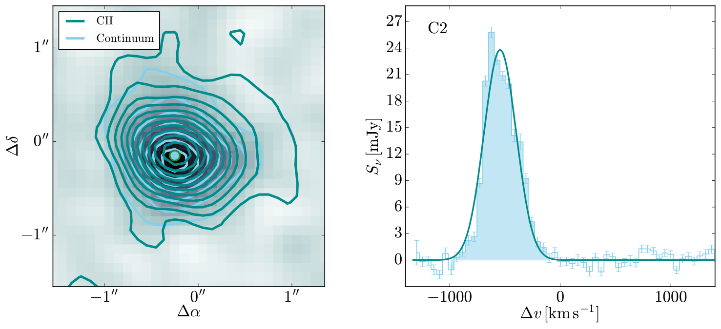

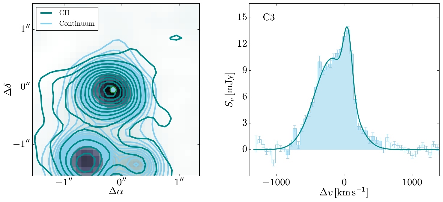

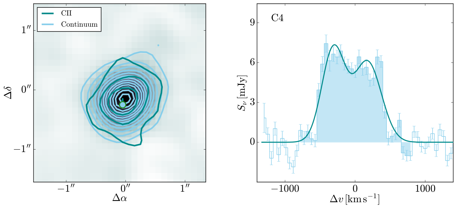


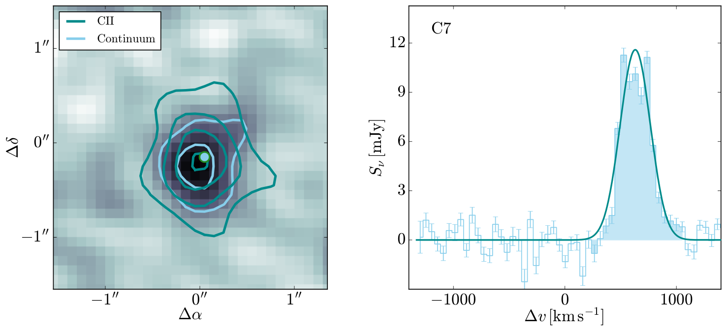


Appendix B High-resolution imaging
We provide continuum cut-outs of our sources obtained from the high-resolution Band 7 imaging. Line-free channels were determined from our deeper Cycle 5 data by fitting Gaussian profiles to each spectrum (see Section 3.4) and stacked. Sérsic profiles were fit to all sources detected in these images above 3, and half-light radii were estimated from the fits.
The left panels show these stacked images with 2 and 3 countours, then increasing in steps of 3, with positions found in the Cycle 5 data shown as blue points and positions found from the Sérsic profiles shown as red points. The red bars indicated the sizes of the half-light radii resulting from the Sérsic profiles, and best-fitting half-light radii and Sérsic indices are shown in the top left. For source NL1 we provide the best-fitting half-light radius in units of arcseconds (as the redshift of this source cannot be confirmed), otherwise the best-fitting half-light radii are in units of kiloparsecs. The middle panels show our Sérsic profile models, and the right panels show the residuals. For sources below 3, where did not attempt to fit Sérsic profiles, we leave the middle panel blank. We also note that source C7 resolves into a complicated structure, possibly a pair of merging galaxies, and we do not attempt to fit a Sérsic profile and measure a half-light radius for it.


