Wave propagation modeling in periodic elasto-thermo-diffusive materials via multifield asymptotic homogenization

The increasing need of energy diversification and employment of alternative and renewable energy sources motivates the growth in the use of fuel cells as power generating systems. Substitution of conventional fuel combustion with an electrochemical reaction in order to generate electricity make fuel cells clean and sustainable energy devices, nowadays exploited for a wide range of applications, from powering satellites to generating power for vehicles and buildings. Fuel cells consist of two porous heat resistant electrodes, the negative one (anode) and the positive one (cathode), undergoing electrochemical reaction in order to produce an electric current. They are sandwiched around a porous electrolyte, which is the ion conductor. Fuel cells differ according to the electrolyte employed, which influences the type of occurring electrochemical reaction, of the catalyst, and of the fuel, thus achieving distinct levels of efficiency (Brandon and Brett 2006). In this context, Solid Oxide Fuel Cells (SOFCs) are characterized by having a doped, solid, ceramic material to form the electrolyte and they excel for their high electrical efficiency and low operating costs (Zhu and Deevi 2003; Bove and Ubertini 2008). The cathode of SOFCs is supplied both with oxygen, acting as the oxidant, and electrons coming from the external electrical circuit. Oxygen ions intercalate into the electrolyte as a consequence of the reduction process taking place at the cathode side. Through the solid electrolyte, negative oxygen ions are therefore conducted from the cathode to the anode, where they combine with the hydrogen fuel, thus generating both water and electrons as products of the oxidation reaction. Electrical current is hence generated by electrons travelling along the external circuit and then reentering into the cathode material. In addition, every single cell is characterized by flow channels for air and fuel and by a metallic or ceramic interconnect separator, which allows connecting cells in series with the aim to produce sufficient voltage for the practical use.

Macroscopic engineering response of such multiphase materials is strongly influenced by the mechanics and physics occurring at the microscale, whose characteristic size is very small compared to the structural one. For this reason a numerical analysis of microstructured devices like a SOFCs stack could reveal extremely challenging in terms of computational and temporal resources (Hajimolana et al. 2011; Dev et al. 2014). When scales separation holds, homogenization techniques result to be remarkably useful in order to provide an accurate and concise description of the medium which properly take into account the behavior and the mechanical response of the microstructure. The application of homogenization methods and multiscale modelings allows avoiding the demanding numerical computation of the whole heterogeneous medium leading to the identification of effective macroscopic properties for the equivalent continuum. In order to study the overall properties of composite materials, numerous homogenization approaches have been provided over the last decades, which can be divided in asymptotic techniques (Sanchez-Palencia 1974; Bensoussan et al. 1978; Bakhvalov and Panasenko 1984; Gambin and Kröner 1989; Allaire 1992; Bacigalupo 2014; Fantoni et al. 2017; Fantoni et al. 2018), variational-asymptotic techniques (Smyshlyaev and Cherednichenko 2000; Peerlings and Fleck 2004; Bacigalupo and Gambarotta 2014), and numerous identification approaches including the analytical (Bigoni and Drugan 2007; Milton and Willis 2007; Bacca et al. 2013a; Bacca et al. 2013b; Bacca et al. 2013c; Nassar et al. 2015; Bacigalupo et al. 2018) and computational methods (Forest and Sab 1998; Ostoja-Starzewski et al. 1999; Feyel and Chaboche 2000; Kouznetsova et al. 2002; Forest 2002; Feyel 2003; Kouznetsova et al. 2004; Lew et al. 2004; Kaczmarczyk et al. 2008; Yuan et al. 2008; Scarpa et al. 2009; Bacigalupo and Gambarotta 2010; Forest and Trinh 2011; De Bellis and Addessi 2011; Addessi et al. 2013; Zäh and Miehe 2013; Salvadori et al. 2014; Trovalusci et al. 2015). The present study is devoted to provide a multifield asymptotic homogenization technique for periodic thermo-diffusive materials considering as periodic cell the typical SOFC building block. An accurate prediction of the overall response of SOFCs is of crucial importance in order to guarantee the satisfaction of design requirements and the reliability of the entire system. Battery devices like SOFCs, in fact, are subjected to severe stresses due to high operating temperatures ($600-1000$) (Pitakthapanaphong and Busso 2005) and intense particle diffusion, which could compromise their efficiency in terms of power generation and energy conversion, ultimately impacting on their failure behavior (Atkinson and Sun 2007; Kuebler et al. 2010; Delette et al. 2013). Previous numerical models of SOFCs focused on electrochemical aspects can be found in (Kakac et al. 2007; Colpan et al. 2008), while mechanical properties of each phase forming the composite battery device are presented in (Hasanov et al. 2011). Latterly, different multiscale modeling of SOFCs have been provided focusing on computational homogenization (Kim et al. 2009; Muramatsu et al. 2015; Molla et al. 2016), asymptotic first-order homogenization of thermo-mechanical properties (Bacigalupo et al. 2016), and asymptotic non local homogenization of elastic properties (Bacigalupo et al. 2014) where the influence of temperature upon local and non local overall constitutive tensors has been studied. Furthermore, an investigation of the complex frequency band structure of periodic SOFCs based on a micromechanical perspective has been recently presented by one of the author in (Bacigalupo et al. 2019). Nevertheless, to the best of authors’ knowledge, a rigorous quantitative multiscale description of mechanical, thermal, and diffusive properties of SOFC-like material and their coupling is still missing. In the followings, down-scaling relations are provided. They relate the microfields, specifically the displacement, the relative temperature and the chemical potential to the macroscopic fields and their gradients by means of perturbation functions. These lasts are regular, periodic functions derived through the resolution of recursive, non homogeneous differential problems, known as cell problems, obtained inserting an asymptotic expansion of the microfields in powers of the microstructural length scale into the local balance equations and reordering at the different orders of the micro characteristic size. Following the rigorous approach described in (Smyshlyaev and Cherednichenko 2000; Bacigalupo 2014), average field equations of infinite order are obtained from the substitution of down-scaling relations into micro governing field equations. A formal solution of the average field equations of infinite order can be attained by performing an asymptotic expansion of the macrofields in powers of the micro length scale, and truncation of resulting equations to the zeroth order allows characterizing field equations of the first-order equivalent medium for the class of periodic thermo-diffusive materials considered. Coefficients of obtained field equations are related to the overall constitutive tensors, whose expression is provided in closed form in terms of perturbation functions and microscopic constitutive properties.

With the aim of investigating the dispersive free waves propagation within the periodic microstructured material, bilateral Laplace transform in time and Fourier transform in space are applied to field equations of the homogenized medium, thus obtaining a quadratic generalized eigenvalue problem, whose solution characterizes the complex frequency band structure of the first-order equivalent medium. The validity of the proposed approach is assessed by comparing the obtained complex frequency spectra with the ones relative to the heterogeneous thermo-diffusive material. In this case, a generalization of the Floquet-Bloch theory is employed, which allows determining dispersion properties of the heterogeneous material by solving a generalized quadratic eigenvalue problem over the periodic cell endowed with Floquet-Bloch boundary conditions. Finally, an asymptotic approximation of the complex spectrum for the first-order equivalent medium is performed via perturbative technique. This allows achieving a parametric approximation of the complex frequency in powers of the wave vector in terms of the overall constitutive parameters and obtained explicit dispersion curves demonstrate to match very well with the ones relative to the homogenized medium. The work is organized as follows: Section describes the governing microscopic field equations and recursive differential problems obtained through asymptotic expansion of the microfields in powers of the microstructural length scale. Cell problems and relative perturbation functions at the different orders of the micro characteristic size are detailed in Section . Section is devoted to the determination of down-scaling and up-scaling relations, while in Section field equations of the first-order equivalent continuum are presented and overall constitutive tensors are provided in closed form. The determination of complex frequency band structure for the first-order homogenized medium is described in Section , together with its asymptotic approximation via perturbative method in Section . In order to evaluate the capabilities of the proposed method a representative example is performed in Section , where the complex frequency band structure and its asymptotic approximation are provided for the equivalent continuum in relation to a typical SOFC and obtained results are compared with the ones of the relative heterogeneous periodic cell. Final remarks are then proposed in Section .

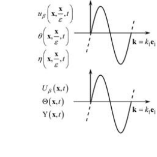
Under the assumption of small strains, the heterogeneous microstructured composite material depicted in figure is described as a linear thermo-diffusive Cauchy medium (Nowacki 1974a; Nowacki 1974b; Nowacki 1974c). In a two-dimensional perspective, as represented in figure , vector $\mathbf{x}=x_{1}\,\mathbf{e}_{1}+x_{2}\,\mathbf{e}_{2}$ defines the position of each material point in the orthogonal reference system $\{O,\mathbf{e}_{1},\mathbf{e}_{2}\}$. Micro fields characterizing the first-order continuum are the displacement field $\mathbf{u}(\mathbf{x},t)=u_{i}(\mathbf{x},t)\mathbf{e}_{i}$, relative temperature field $\theta(\mathbf{x},t)=T(\mathbf{x},t)-T_{0}$ with $T(\mathbf{x},t)$ the absolute temperature and $T_{0}$ a reference stress free temperature, and chemical potential field $\eta(\mathbf{x},t)$. Being $\varepsilon$ the characteristic size of the microstructure, two periodicity vectors $\mathbf{v}_{1}=d_{1}\,\mathbf{e}_{1}=\varepsilon\,\mathbf{e}_{1}$ and $\mathbf{v}_{2}=d_{2}\,\mathbf{e}_{2}=\delta\varepsilon\,\mathbf{e}_{2}$ identify the periodic cell $\mathcal{A}=[0,\varepsilon]\times[0,\delta\varepsilon]$ (figure -(b)). Rescaling cell $\mathcal{A}$ by the length $\varepsilon$, the periodic microstructure is obtained by spanning the nondimensional unit cell $\mathcal{Q}=[0,1]\times[0,\delta]$, as depicted in figure -(c).

The separation between the macro and the micro scales is mathematically described by two distinct variables, namely the macroscopic (or slow) one $\mathbf{x}\in\mathcal{A}$ and the microscopic (or fast) one ${\bm{\xi}}=\mathbf{x}/\varepsilon\in\mathcal{Q}$ (Bakhvalov and Panasenko 1984; Smyshlyaev and Cherednichenko 2000; Peerlings and Fleck 2004; Bacigalupo 2014). Micro-stress tensor ${\bm{\sigma}}(\mathbf{x},t)=\sigma_{ij}\,(\mathbf{x},t)\mathbf{e}_{i}\otimes\mathbf{e}_{j}$, micro heat flux vector $\mathbf{q}(\mathbf{x},t)=q_{i}\,(\mathbf{x},t)\mathbf{e}_{i}$, and mass flux vector $\mathbf{j}(\mathbf{x},t)=j_{i}\,(\mathbf{x},t)\mathbf{e}_{i}$ are determined by the coupled constitutive relations (Nowacki 1974a; Nowacki 1974b; Nowacki 1974c)

where symbol ${\bm{\varepsilon}}(\mathbf{x},t)=sym\nabla\mathbf{u}(\mathbf{x},t)$ is the micro small strains tensor and superscript $m$ refers to the microscale. In equations (1a)-(1c) $\mathfrak{C}=C_{ijkl}\left({\bm{\xi}}=\frac{\mathbf{x}}{\varepsilon}\right)\mathbf{e}_{i}\otimes\mathbf{e}_{j}\otimes\mathbf{e}_{k}\otimes\mathbf{e}_{l}$ is the fourth order micro elasticity tensor having major and minor symmetries, ${\bm{\alpha}}=\alpha_{ij}\left({\bm{\xi}}=\frac{\mathbf{x}}{\varepsilon}\right)\mathbf{e}_{i}\otimes\mathbf{e}_{j}$ is the symmetric second order micro thermal dilatation tensor, ${\bm{\beta}}=\beta_{ij}\left({\bm{\xi}}=\frac{\mathbf{x}}{\varepsilon}\right)\mathbf{e}_{i}\otimes\mathbf{e}_{j}$ is the symmetric second order micro diffusive expansion tensor, ${\bm{K}}=K_{ij}\left({\bm{\xi}}=\frac{\mathbf{x}}{\varepsilon}\right)\mathbf{e}_{i}\otimes\mathbf{e}_{j}$ is the symmetric second order micro heat conduction tensor, and ${\bm{D}}=D_{ij}\left({\bm{\xi}}=\frac{\mathbf{x}}{\varepsilon}\right)\mathbf{e}_{i}\otimes\mathbf{e}_{j}$ is the symmetric second order micro mass diffusion tensor. Micro constitutive tensors are all $\mathcal{Q}$-periodic and dependent upon the fast variable ${\bm{\xi}}$. Local balance equations hold

where source terms depend exclusively upon the slow variable and time and are represented by body forces $\mathbf{b}(\mathbf{x},t)$, heat sources $r(\mathbf{x},t)$, and mass sources $s(\mathbf{x},t)$. Source terms are here assumed to be $\mathcal{L}$-periodic and to have vanishing mean values on $\mathcal{L}$, where, indicating with $L$ the structural characteristic size, the portion $\mathcal{L}=[0,L]\times[0,\delta L]$ can be considered as truly representative of the whole medium. In this regard, size $L$ has to be much greater than the microstructural one ($L\gg\varepsilon$) so that the scales separation condition is met. In equations (2a)-(2c) inertial terms are $\mathcal{Q}$-periodic and represented by the mass density $\rho=\rho({\bm{\xi}}=\frac{\mathbf{x}}{\varepsilon})$, material constant $p=p({\bm{\xi}}=\frac{\mathbf{x}}{\varepsilon})$ related to the specific heat at constant strain and to thermo-diffusive effects, and material constant $q=q({\bm{\xi}}=\frac{\mathbf{x}}{\varepsilon})$ related to diffusive effect. Finally, term $\psi=\psi({\bm{\xi}}=\frac{\mathbf{x}}{\varepsilon})$ is a $\mathcal{Q}$-periodic coupling constant measuring the thermo-diffusive effect. Substitution of constitutive equations (1a)-(1c) into local balance relations (2a)-(2c) leads to

For an ideally bonded interface $\Sigma$, the following continuity conditions hold

where $[[f]]=f(\Sigma)-f(\Sigma)$ denotes the discontinuity of the values of a function $f$ at the interface $\Sigma$ between two different phases $i$ and $j$ of periodic cell $\mathcal{A}$ and $\mathbf{n}=n_{j}\,\mathbf{e}_{j}$ represents the outward normal to the interface $\Sigma$. Taking into account the $\mathcal{Q}$-periodicity of micro constitutive tensors and inertial terms, interface conditions (4a)-(4c), and the $\mathcal{L}$-periodicity of source terms, it results that the microscopic fields spatially depend on both the slow and the fast variables $\mathbf{x}$ and ${\bm{\xi}}$ and are expressed as

Rapidly oscillating $\mathcal{Q}$-periodic coefficients of PDEs (3a)-(3c) make their analytical and/or numerical resolution particularly labor intensive. In this sense, homogenization techniques can reveal very useful in replacing the microstructured continuum with an equivalent homogeneous one. In what follows, field equations of a first-order thermo-diffusive equivalent continuum will be characterized and the closed form of overall constitutive tensors will be obtained. By means of a dynamic multi-field asymptotic homogenization technique, the global behavior of the composite material will be concisely and accurately described, thus overcoming the computational burden of resolution of equations (3a)-(3c) and facilitating their analytical resolution on simple domains. Macroscopic fields of the equivalent homogenized medium, are denoted as $\mathbf{U}(\mathbf{x},t)=U_{i}(\mathbf{x},t)\mathbf{e}_{i}$ for the displacement, $\Theta(\mathbf{x},t)$ for the relative temperature and $\Upsilon(\mathbf{x},t)$ for chemical potential. They only depend in space upon the macroscopic slow variable $\mathbf{x}$ and they result to be $\mathcal{L}$-periodic if source terms are $\mathcal{L}$-periodic.

References

• Addessi et al. (2013) Addessi, D., De Bellis, M., Sacco, E., 2013. Micromechanical analysis of heterogeneous materials subjected to overall cosserat strains. Mechanics Research Communications 54, 27–34.
• Allaire (1992) Allaire, G., 1992. Homogenization and two-scale convergence. SIAM Journal of Mathematical Analisys 23, 1482–1518.
• Atkinson and Sun (2007) Atkinson, A., Sun, B., 2007. Residual stress and thermal cycling of planar solid oxide fuel cells. Materials Science and Technology 23, 1135–1143.
• Bacca et al. (2013a) Bacca, M., Bigoni, D., Dal Corso, F., Veber, D., 2013a. Mindlin second-gradient elastic properties from dilute two-phase cauchy-elastic composites. part i: Closed form expression for the effective higher-order constitutive tensor. International Journal of Solids and Structures 50(24), 4010–4019.
• Bacca et al. (2013b) Bacca, M., Bigoni, D., Dal Corso, F., Veber, D., 2013b. Mindlin second-gradient elastic properties from dilute two-phase cauchy-elastic composites part ii: Higher-order constitutive properties and application cases. international journal of solids and structures. International Journal of Solids and Structures 50(24), 4020–4029.
• Bacca et al. (2013c) Bacca, M., Dal Corso, F., Veber, D., Bigoni, D., 2013c. Anisotropic effective higher-order response of heterogeneous cauchy elastic materials. Mechanics Research Communications 54, 63–71.
• Bacigalupo (2014) Bacigalupo, A., 2014. Second-order homogenization of periodic materials based on asymptotic approximation of the strain energy: formulation and validity limits. Meccanica 49(6), 1407–1425.
• Bacigalupo et al. (2019) Bacigalupo, A., De Bellis, M.L., Gnecco, G., 2019. Complex frequency band structure of periodic thermo-diffusive materials by floquet-bloch theory. Acta Mechanica 230, 3339–3363.
• Bacigalupo and Gambarotta (2010) Bacigalupo, A., Gambarotta, L., 2010. Second-order computational homogenization of heterogeneous materials with periodic microstructure. ZAMM–Journal of Applied Mathematics and Mechanics/Zeitschrift für Angewandte Mathematik und Mechanik 90, 796–811.
• Bacigalupo and Gambarotta (2014) Bacigalupo, A., Gambarotta, L., 2014. Computational dynamic homogenization for the analysis of dispersive waves in layered rock masses with periodic fractures. Computers and Geotechnics 56, 61–68.
• Bacigalupo and Lepidi (2016) Bacigalupo, A., Lepidi, M., 2016. High-frequency parametric approximation of the floquet-bloch spectrum for anti-tetrachiral materials. International Journal of Solids and Structures 97, 575–592.
• Bacigalupo et al. (2014) Bacigalupo, A., Morini, L., Piccolroaz, A., 2014. Effective elastic properties of planar sofcs: A non-local dynamic homogenization approach. International Journal of Hydrogen Energy 39(27), 15017–15030.
• Bacigalupo et al. (2016) Bacigalupo, A., Morini, L., Piccolroaz, A., 2016. Multiscale asymptotic homogenization analysis of thermo-diffusive composite materials. International Journal of Solids and Structures 85-86, 15–33.
• Bacigalupo et al. (2018) Bacigalupo, A., Paggi, M., Dal Corso, F., Bigoni, D., 2018. Identification of higher-order continua equivalent to a cauchy elastic composite. Mechanics Research Communications 93, 11–22.
• Bakhvalov and Panasenko (1984) Bakhvalov, N., Panasenko, G., 1984. Homogenization: Averaging Processes in Periodic Media. Kluwer Academic Publishers, Dordrecht-Boston-London.
• Bensoussan et al. (1978) Bensoussan, A., Lions, J., Papanicolaou, G., 1978. Asymptotic analysis for periodic structures. North-Holland, Amsterdam.
• Bigoni and Drugan (2007) Bigoni, D., Drugan, W., 2007. Analytical derivation of cosserat moduli via homogenization of heterogeneous elastic materials. Journal of Applied Mechanics 74(4), 741–753.
• Bloch (1929) Bloch, F., 1929. Über die quantenmechanik der elektronen in kristallgittern. Zeitschrift für physik 52, 555–600.
• Bove and Ubertini (2008) Bove, R., Ubertini, S., 2008. Modeling solid oxide fuel cells: methods, procedures and techniques. Springer Science & Business Media.
• Brandon and Brett (2006) Brandon, N., Brett, D., 2006. Engineering porous materials for fuel cell applications. Philosophical Transactions of the Royal Society A: Mathematical, Physical and Engineering Sciences 364, 147–159.
• Brillouin (1953) Brillouin, L., 1953. Wave propagation in periodic structures: electric filters and crystal lattices .
• Colpan et al. (2008) Colpan, C.O., Dincer, I., Hamdullahpur, F., 2008. A review on macro-level modeling of planar solid oxide fuel cells. International Journal of Energy Research 32, 336–355.
• De Bellis and Addessi (2011) De Bellis, M.L., Addessi, D., 2011. A cosserat based multi-scale model for masonry structures. International Journal for Multiscale Computational Engineering 9, 543.
• Delette et al. (2013) Delette, G., Laurencin, J., Usseglio-Viretta, F., Villanova, J., Bleuet, P., Lay-Grindler, E., Le Bihan, T., 2013. Thermo-elastic properties of sofc/soec electrode materials determined from three-dimensional microstructural reconstructions. International journal of hydrogen energy 38, 12379–12391.
• Dev et al. (2014) Dev, B., Walter, M.E., Arkenberg, G.B., Swartz, S.L., 2014. Mechanical and thermal characterization of a ceramic/glass composite seal for solid oxide fuel cells. Journal of Power Sources 245, 958–966.
• Fantoni et al. (2017) Fantoni, F., Bacigalupo, A., Paggi, M., 2017. Multi-field asymptotic homogenization of thermo-piezoelectric materials with periodic microstructure. International Journal of Solids and Structures 120, 31–56.
• Fantoni et al. (2018) Fantoni, F., Bacigalupo, A., Paggi, M., 2018. Design of thermo-piezoelectric microstructured bending actuators via multi-field asymptotic homogenization. International Journal of Mechanical Sciences 146, 319–336.
• Feyel (2003) Feyel, F., 2003. A multilevel finite element method (fe2) to describe the response of highly non-linear structures using generalized continua. Computer Methods in applied Mechanics and engineering 192, 3233–3244.
• Feyel and Chaboche (2000) Feyel, F., Chaboche, J., 2000. FE multiscale approach for modelling the elastoviscoplastic behaviour of long fibre SiC/Ti composite materials. Computer Methods in Applied Mechanics Engineering 183, 309–330.
• Floquet (1883) Floquet, G., 1883. Sur les équations différentielles linéaires à coefficients périodiques, in: Annales scientifiques de l’École normale supérieure, pp. 47–88.
• Forest (2002) Forest, S., 2002. Homogenization methods and the mechanics of generalized continua-part 2. Theoretical and applied mechanics 28, 113–144.
• Forest and Sab (1998) Forest, S., Sab, K., 1998. Cosserat overall modeling of heterogeneous materials. Mechanics Research Communications 25(4), 449–454.
• Forest and Trinh (2011) Forest, S., Trinh, D., 2011. Generalized continua and non‐homogeneous boundary conditions in homogenisation methods. ZAMM‐Journal of Applied Mathematics and Mechanics/Zeitschrift für Angewandte Mathematik und Mechanik 91(2), 90–109.
• Gambin and Kröner (1989) Gambin, B., Kröner, E., 1989. Higher order terms in the homogenized stress‐strain relation of periodic elastic media. physica status solidi (b). International Journal of Engineering Science 151(2), 513–519.
• Hajimolana et al. (2011) Hajimolana, S.A., Hussain, M.A., Daud, W.A.W., Soroush, M., Shamiri, A., 2011. Mathematical modeling of solid oxide fuel cells: A review. Renewable and Sustainable Energy Reviews 15, 1893–1917.
• Hasanov et al. (2011) Hasanov, R., Smirnova, A., Gulgazli, A., Kazimov, M., Volkov, A., Quliyeva, V., Vasylyev, O., Sadykov, V., 2011. Modeling design and analysis of multi-layer solid oxide fuel cells. International journal of hydrogen energy 36, 1671–1682.
• Kaczmarczyk et al. (2008) Kaczmarczyk, L., Pearce, C.J., Bićanić, N., 2008. Scale transition and enforcement of rve boundary conditions in second-order computational homogenization. International Journal for Numerical Methods in Engineering 74, 506–522.
• Kakac et al. (2007) Kakac, S., Pramuanjaroenkij, A., Zhou, X.Y., 2007. A review of numerical modeling of solid oxide fuel cells. International journal of hydrogen energy 32, 761–786.
• Kim et al. (2009) Kim, J.H., Liu, W.K., Lee, C., 2009. Multi-scale solid oxide fuel cell materials modeling. Computational Mechanics 44, 683–703.
• Kouznetsova et al. (2002) Kouznetsova, V., Geers, M., Brekelmans, W., 2002. Multi-scale constitutive modelling of heterogeneous materials with a gradient-enhanced computational homogenization scheme. International Journal for Numerical Methods in Engineering 54, 1235–1260.
• Kouznetsova et al. (2004) Kouznetsova, V., Geers, M., Brekelmans, W., 2004. Multi-scale second-order computational homogenization of multi-phase materials: a nested finite element solution strategy. Computer Methods in Applied Mechanics and Engineering 193(48), 5525–5550.
• Kuebler et al. (2010) Kuebler, J., Vogt, U.F., Haberstock, D., Sfeir, J., Mai, A., Hocker, T., Roos, M., Harnisch, U., 2010. Simulation and validation of thermo-mechanical stresses in planar sofcs. Fuel Cells 10, 1066–1073.
• Langley (1993) Langley, R., 1993. A note on the force boundary conditions for two-dimensional periodic structures with corner freedoms. Journal of Sound and Vibration 167, 377–381.
• Lew et al. (2004) Lew, T., Scarpa, F., Worden, K., 2004. Homogenisation metamodelling of perforated plates. Strain 40, 103–112.
• Mead (1973) Mead, D., 1973. A general theory of harmonic wave propagation in linear periodic systems with multiple coupling. Journal of Sound and Vibration 27, 235–260.
• Mehrabadi and Cowin (1990) Mehrabadi, M., Cowin, S., 1990. Eigentensors of linear anisotropic elastic materials. The Quarterly Journal of Mechanics and Applied Mathematics 43(1), 15–41.
• Milton and Willis (2007) Milton, G.W., Willis, J.R., 2007. On modifications of newton’s second law and linear continuum elastodynamics. Proceedings of the Royal Society A: Mathematical, Physical and Engineering Sciences 463, 855–880.
• Molla et al. (2016) Molla, T.T., Kwok, K., Frandsen, H.L., 2016. Efficient modeling of metallic interconnects for thermo-mechanical simulation of sofc stacks: homogenized behaviors and effect of contact. International Journal of Hydrogen Energy 41, 6433–6444.
• Muramatsu et al. (2015) Muramatsu, M., Terada, K., Kawada, T., Yashiro, K., Takahashi, K., Takase, S., 2015. Characterization of time-varying macroscopic electro-chemo-mechanical behavior of sofc subjected to ni-sintering in cermet microstructures. Computational Mechanics 56, 653–676.
• Nassar et al. (2015) Nassar, H., He, Q.C., Auffray, N., 2015. Willis elastodynamic homogenization theory revisited for periodic media. Journal of the Mechanics and Physics of Solids 77, 158–178.
• Nowacki (1974a) Nowacki, W., 1974a. Dynamical problem of thermodiffusion in solids. 1. Bulletin de lácademie polonaise des sciences-serie des sciences techniques 22, 55–64.
• Nowacki (1974b) Nowacki, W., 1974b. Dynamical problem of thermodiffusion in solids. 2. Bulletin de lácademie polonaise des sciences-serie des sciences techniques 22, 205–211.
• Nowacki (1974c) Nowacki, W., 1974c. Dynamical problem of thermodiffusion in solids. 3. Bulletin de lácademie polonaise des sciences-serie des sciences techniques 22, 257–266.
• Ostoja-Starzewski et al. (1999) Ostoja-Starzewski, M., Boccara, S.D., Jasiuk, I., 1999. Couple-stress moduli and characteristic length of a two-phase composite. Mechanics Research Communications 26, 387–396.
• Paley and Wiener (1934) Paley, R., Wiener, N., 1934. Fourier transforms in the complex domain. volume 19. American Mathematical Soc.
• Peerlings and Fleck (2004) Peerlings, R., Fleck, N., 2004. Computational evaluation of strain gradient elasticity constants. International Journal for Multiscale Computational Engineering 2(4).
• Phani et al. (2006) Phani, A.S., Woodhouse, J., Fleck, N., 2006. Wave propagation in two-dimensional periodic lattices. The Journal of the Acoustical Society of America 119, 1995–2005.
• Pitakthapanaphong and Busso (2005) Pitakthapanaphong, S., Busso, E., 2005. Finite element analysis of the fracture behaviour of multi-layered systems used in solid oxide fuel cell applications. Modelling and Simulation in Materials Science and Engineering 13, 531.
• Salvadori et al. (2014) Salvadori, A., Bosco, E., Grazioli, D., 2014. A computational homogenization approach for Li-ion battery cells. Part 1 - Formulation. Journal of the Mechanics and Physics of Solids 65, 114–137. doi:http://dx.doi.org/10.1016/j.jmps.2013.08.010.
• Sanchez-Palencia (1974) Sanchez-Palencia, E., 1974. Comportements local et macroscopique d’un type de milieux physiques heterogenes. International Journal of Engineering Science 12(4), 331–351.
• Scarpa et al. (2009) Scarpa, F., Adhikari, S., Phani, A.S., 2009. Effective elastic mechanical properties of single layer graphene sheets. Nanotechnology 20, 065709.
• Smyshlyaev and Cherednichenko (2000) Smyshlyaev, V., Cherednichenko, K., 2000. On rigorous derivation of strain gradient effects in the overall behaviour of periodic heterogeneous media. Journal of the Mechanics and Physics of Solids 48(6), 1325–1357.
• Trovalusci et al. (2015) Trovalusci, P., Ostoja-Starzewski, M., De Bellis, M.L., Murrali, A., 2015. Scale-dependent homogenization of random composites as micropolar continua. European Journal of Mechanics-A/Solids 49, 396–407.
• Yuan et al. (2008) Yuan, X., Tomita, Y., Andou, T., 2008. A micromechanical approach of nonlocal modeling for media with periodic microstructures. Mechanics Research Communications 35, 126–133.
• Zäh and Miehe (2013) Zäh, D., Miehe, C., 2013. Computational homogenization in dissipative electro-mechanics of functional materials. Computer Methods in Applied Mechanics and Engineering 267, 487–510.
• Zhu and Deevi (2003) Zhu, W., Deevi, S., 2003. A review on the status of anode materials for solid oxide fuel cells. Materials Science and Engineering: A 362, 228–239.
Appendix A. Proof of equivalence among thermo-diffusive homogeneous tensors
In the present Section the following equivalences between the components of overall constitutive tensors that appear in the average field equations of infinite order () are demonstrated in detail
n~p​q1=m~p​q1,n^p​q1=w~p​q1,m^=w^.\tilde{n}_{pq_{1}}=\tilde{m}_{pq_{1}},\hskip 5.69046pt\hat{n}_{pq_{1}}=\tilde{w}_{pq_{1}},\hskip 5.69046pt\hat{m}=\hat{w}. (113)
This allows relating components of tensors 𝐧~=n~p​q1​𝐞p⊗𝐞q1\tilde{\mathbf{n}}=\tilde{n}_{pq_{1}}\,\mathbf{e}_{p}\otimes\mathbf{e}_{q_{1}}, 𝐦~=m~p​q1​𝐞p⊗𝐞q1\tilde{\mathbf{m}}=\tilde{m}_{pq_{1}}\,\mathbf{e}_{p}\otimes\mathbf{e}_{q_{1}}, 𝐧^=n^p​q1​𝐞p⊗𝐞q1\hat{\mathbf{n}}=\hat{n}_{pq_{1}}\,\mathbf{e}_{p}\otimes\mathbf{e}_{q_{1}}, 𝐰~=w~p​q1​𝐞p⊗𝐞q1\tilde{\mathbf{w}}=\tilde{w}_{pq_{1}}\,\mathbf{e}_{p}\otimes\mathbf{e}_{q_{1}} to the corresponding ones of overall constitutive tensors 𝜶{\bm{\alpha}} and 𝜷{\bm{\beta}} and to relate constants m^\hat{m} and w^\hat{w} to the overall coupling constant ψ\psi.
Proof of 𝐧~=𝐦~\tilde{\mathbf{n}}=\tilde{\mathbf{m}}
Components of tensors 𝐧~\tilde{\mathbf{n}} and 𝐦~\tilde{\mathbf{m}} come from the known terms of cell problems (3) and (3), respectively, and have the following expressions
n~p​q1=⟨αp​q1−Cp​q1​k​j,j​N~k,j⟩,\displaystyle\tilde{n}_{pq_{1}}=\left\langle\alpha_{pq_{1}}-C_{pq_{1}kj,j}\tilde{N}_{k,j}\right\rangle, (114a)
m~p​q1=⟨αp​q1+αi​q2​Ni​p​q1,q2⟩.\displaystyle\tilde{m}_{pq_{1}}=\left\langle\alpha_{pq_{1}}+\alpha_{iq_{2}}N_{ipq_{1},q_{2}}\right\rangle. (114b)
The weak form of the first mechanical cell problem (3) at the order ε\varepsilon
(Cp​j​k​lNk​i​q1,l),j+Cp​j​i​q1,j=0,\left(C_{pjkl}N_{kiq_{1},l}\right)_{,j}+C_{pjiq_{1},j}=0, (115)
can be written in the following way, considering as test function the perturbation function N~p\tilde{N}_{p}
⟨[(Cp​j​k​lNk​i​q1,l),j+Cp​j​i​q1,j]N~p⟩=0.\left\langle\left[\left(C_{pjkl}N_{kiq_{1},l}\right)_{,j}+C_{pjiq_{1},j}\right]\tilde{N}_{p}\right\rangle=0. (116)
Divergence theorem and 𝒬\mathcal{Q}-periodicity of micro constitutive tensors and perturbation functions, allow writing equation () as
⟨[Cp​j​k​l​Nk​i​q1,l+Cp​j​i​q1]​N~p,j⟩=0.\left\langle\left[C_{pjkl}N_{kiq_{1},l}+C_{pjiq_{1}}\right]\tilde{N}_{p,j}\right\rangle=0. (117)
Adding vanishing term () to expression (114a), one obtains
n~p​q1=⟨αp​q1−Cp​q1​i​l,l​N~i,l+Ci​j​k​l​Ni​p​q1,j​N~k,l+Ck​l​p​q1​N~k,l⟩=⟨αp​q1+Ck​l​i​k​N~k,l​Ni​p​q1,j⟩.\tilde{n}_{pq_{1}}=\left\langle\alpha_{pq_{1}}-C_{pq_{1}il,l}\tilde{N}_{i,l}+C_{ijkl}N_{ipq_{1},j}\tilde{N}_{k,l}+C_{klpq_{1}}\tilde{N}_{k,l}\right\rangle=\left\langle\alpha_{pq_{1}}+C_{klik}\tilde{N}_{k,l}N_{ipq_{1},j}\right\rangle. (118)
Analogously, from the second mechanical cell problem (3) at the order ε\varepsilon
(Ci​j​k​lN~k,l),j−αi​j,j=0,\left(C_{ijkl}\tilde{N}_{k,l}\right)_{,j}-\alpha_{ij,j}=0, (119)
the following weak form can be written in terms of test function Ni​p​q1N_{ipq_{1}}
⟨[(Ci​j​k​lN~k,l),j−αi​j,j]Ni​p​q1⟩=0.\left\langle\left[\left(C_{ijkl}\tilde{N}_{k,l}\right)_{,j}-\alpha_{ij,j}\right]N_{ipq_{1}}\right\rangle=0. (120)
Expression () can be transformed into
⟨[Ci​j​k​l​N~k,l−αi​j]​Ni​p​q1,j=0⟩,\left\langle\left[C_{ijkl}\tilde{N}_{k,l}-\alpha_{ij}\right]N_{ipq_{1},j}=0\right\rangle, (121)
thanks to divergence theorem and 𝒬\mathcal{Q}-periodicity of micro tensors and perturbation functions. Adding () to (114b) yields
m~p​q1=⟨αp​q1+αi​q2​Ni​p​q1,q2+Ci​j​k​l​N~k,l​Ni​p​q1,j−αi​j​Ni​p​q1,j⟩=⟨αp​q1+Ci​j​k​l​N~k,l​Ni​p​q1,j⟩,\tilde{m}_{pq_{1}}=\left\langle\alpha_{pq_{1}}+\alpha_{iq_{2}}N_{ipq_{1},q_{2}}+C_{ijkl}\tilde{N}_{k,l}N_{ipq_{1},j}-\alpha_{ij}N_{ipq_{1},j}\right\rangle=\left\langle\alpha_{pq_{1}}+C_{ijkl}\tilde{N}_{k,l}N_{ipq_{1},j}\right\rangle, (122)
from which identity n^p​q1=w~p​q1\hat{n}_{pq_{1}}=\tilde{w}_{pq_{1}} follows.
Proof of 𝐧^=𝐰~\hat{\mathbf{n}}=\tilde{\mathbf{w}}
Components np​q1n_{pq_{1}} and w~p​q1\tilde{w}_{pq_{1}} are related to the known terms of cell problems (3) and (3), namely
n^p​q1=⟨βp​q1−Cp​q1​k​j​N^k,j⟩,\displaystyle\hat{n}_{pq_{1}}=\left\langle\beta_{pq_{1}}-C_{pq_{1}kj}\hat{N}_{k,j}\right\rangle, (123a)
w~p​q1=⟨βp​q1+βi​q2​N^i​p​q1,q2⟩.\displaystyle\tilde{w}_{pq_{1}}=\left\langle\beta_{pq_{1}}+\beta_{iq_{2}}\hat{N}_{ipq_{1},q_{2}}\right\rangle. (123b)
Given the first mechanical cell problem (3) at the order ε\varepsilon
(Cp​j​k​lNk​i​q1,l),j+Cp​j​i​q1,j=0,\left(C_{pjkl}N_{kiq_{1},l}\right)_{,j}+C_{pjiq_{1},j}=0, (124)
its weak form has expression
⟨[(Cp​j​k​lNk​i​q1,l),j+Cp​j​i​q1,j]N^p⟩=0,\left\langle\left[\left(C_{pjkl}N_{kiq_{1},l}\right)_{,j}+C_{pjiq_{1},j}\right]\hat{N}_{p}\right\rangle=0, (125)
with test function N^p\hat{N}_{p}. Equation () can be written as
⟨[Cp​j​k​l​Nk​i​q1,l+Cp​j​i​q1]​N^p,j⟩=0,\left\langle\left[C_{pjkl}N_{kiq_{1},l}+C_{pjiq_{1}}\right]\hat{N}_{p,j}\right\rangle=0, (126)
for divergence theorem and 𝒬\mathcal{Q}-periodicity of micro constitutive tensors components and weight functions. By adding vanishing term () to equation (123a) one obtains
n^p​q1=⟨βp​q1−Cp​q1​i​l​N^i,l+Ci​j​k​l​Ni​p​q1,j​N^k,l+Ci​l​p​q1​N^i,l⟩=⟨βp​q1+Ci​j​k​l​Ni​p​q1,j​N^k,l⟩.\hat{n}_{pq_{1}}=\left\langle\beta_{pq_{1}}-C_{pq_{1}il}\hat{N}_{i,l}+C_{ijkl}{N}_{ipq_{1},j}\hat{N}_{k,l}+C_{ilpq_{1}}\hat{N}_{i,l}\right\rangle=\left\langle\beta_{pq_{1}}+C_{ijkl}{N}_{ipq_{1},j}\hat{N}_{k,l}\right\rangle. (127)
From cell problem (3) at the order ε\varepsilon
(Ci​j​k​lN^k,l),j−βi​j,j=0,\left(C_{ijkl}\hat{N}_{k,l}\right)_{,j}-\beta_{ij,j}=0, (128)
the following weak form can be derived
⟨[(Ci​j​k​lN^k,l),j−βi​j,j]Ni​p​q1⟩=0,\left\langle\left[\left(C_{ijkl}\hat{N}_{k,l}\right)_{,j}-\beta_{ij,j}\right]N_{ipq_{1}}\right\rangle=0, (129)
considering Ni​p​q1N_{ipq_{1}} as a test function. Analogously to what done before, equation () can be written in the form
⟨[Ci​j​k​l​N^k,l−βi​j]​Ni​p​q1,j⟩=0.\left\langle\left[C_{ijkl}\hat{N}_{k,l}-\beta_{ij}\right]N_{ipq_{1},j}\right\rangle=0. (130)
The sum of () and (123b) leads to
w~p​q1=⟨βp​q1+βi​q2​N^i​p​q1,q2+Ci​j​k​l​N^k,l​Ni​p​q1,j−βi​j​Ni​p​q1,j⟩=⟨βp​q1+Ci​j​k​l​N^k,l​Ni​p​q1,j⟩,\tilde{w}_{pq_{1}}=\left\langle\beta_{pq_{1}}+\beta_{iq_{2}}\hat{N}_{ipq_{1},q_{2}}+C_{ijkl}\hat{N}_{k,l}N_{ipq_{1},j}-\beta_{ij}N_{ipq_{1},j}\right\rangle=\left\langle\beta_{pq_{1}}+C_{ijkl}\hat{N}_{k,l}N_{ipq_{1},j}\right\rangle, (131)
from which equivalence n^p​q1=w~p​q1\hat{n}_{pq_{1}}=\tilde{w}_{pq_{1}} follows.
Proof of m^=w^\hat{m}=\hat{w}
Constants m^\hat{m} and w^\hat{w} come from the known terms of cell problems (58)and (3), namely
m^=⟨ψ+αq1​q2​N^q1,q2⟩,\displaystyle\hat{m}=\left\langle\psi+\alpha_{q_{1}q_{2}}\hat{N}_{q_{1},q_{2}}\right\rangle, (132a)
w^=⟨ψ+βq1​q2​N~q1,q2⟩.\displaystyle\hat{w}=\left\langle\psi+\beta_{q_{1}q_{2}}\tilde{N}_{q_{1},q_{2}}\right\rangle. (132b)
Second mechanical cell problem (3) at the order ε\varepsilon reads
(Ci​j​k​lN~k,l),j−αi​j,j=0,\left(C_{ijkl}\tilde{N}_{k,l}\right)_{,j}-\alpha_{ij,j}=0, (133)
and its weak form, considering N^i\hat{N}_{i} as test function, is
⟨[(Ci​j​k​lN~k,l),j−αi​j,j]N^i⟩=0.\left\langle\left[\left(C_{ijkl}\tilde{N}_{k,l}\right)_{,j}-\alpha_{ij,j}\right]\hat{N}_{i}\right\rangle=0. (134)
Once again, equation () can be written as
⟨[Ci​j​k​l​N~k,l−αi​j]​N^i,j⟩=0,\left\langle\left[C_{ijkl}\tilde{N}_{k,l}-\alpha_{ij}\right]\hat{N}_{i,j}\right\rangle=0, (135)
exploiting divergence theorem and 𝒬\mathcal{Q}-periodicity of perturbation functions and micro constitutive tensors. Adding term () to (132a), one obtains
m^=⟨ψ+αq1​q2​N^q1,q2+Ci​j​k​l​N~k,l​N^i,j−αi​j​N^i,j⟩=⟨ψ+Ci​j​k​l​N^i,j​N~k,l⟩.\hat{m}=\left\langle\psi+\alpha_{q_{1}q_{2}}\hat{N}_{q_{1},q_{2}}+C_{ijkl}\tilde{N}_{k,l}\hat{N}_{i,j}-\alpha_{ij}\hat{N}_{i,j}\right\rangle=\left\langle\psi+C_{ijkl}\hat{N}_{i,j}\tilde{N}_{k,l}\right\rangle. (136)
The weak form of cell problem (3) at the order ε\varepsilon, expressed as
(Ci​j​k​lN^k,l),j−βi​j,j=0,\left(C_{ijkl}\hat{N}_{k,l}\right)_{,j}-\beta_{ij,j}=0, (137)
has the form
⟨[(Ci​j​k​lN^k,l),j−βi​j,j]N~i⟩=0,\left\langle\left[\left(C_{ijkl}\hat{N}_{k,l}\right)_{,j}-\beta_{ij,j}\right]\tilde{N}_{i}\right\rangle=0, (138)
with test function N~i\tilde{N}_{i}. Equation () turns into
⟨[Ci​j​k​l​N^k,l−βi​j]​N^i,j⟩=0,\left\langle\left[C_{ijkl}\hat{N}_{k,l}-\beta_{ij}\right]\hat{N}_{i,j}\right\rangle=0, (139)
for divergence theorem and 𝒬\mathcal{Q}-periodicity of terms involved. The sum of vanishing term () and (132b) leads to
w^=⟨ψ+βq1​q2​N~q1,q2−βi​j​N^i,j+Ci​j​k​l​N^k,l​N^i,j⟩=⟨ψ+Ci​j​k​l​N^k,l​N^i,j⟩.\hat{w}=\left\langle\psi+\beta_{q_{1}q_{2}}\tilde{N}_{q_{1},q_{2}}-\beta_{ij}\hat{N}_{i,j}+C_{ijkl}\hat{N}_{k,l}\hat{N}_{i,j}\right\rangle=\left\langle\psi+C_{ijkl}\hat{N}_{k,l}\hat{N}_{i,j}\right\rangle. (140)
Comparing () and (), the equivalence between constants m^\hat{m} and w^\hat{w} trivially derives.
Appendix B. Fourth order approximation of dispersion functions for the equivalent thermo-diffusive medium
Considering an angular coordinate ϕ=0\phi=0, sensitivities ωi\omega_{i}, with n=1,..,4n=1,..,4 and i=1,…,6i=1,...,6 of table have the closed form detailed below in terms of the overall constitutive tensors components relative to the homogenized thermo-diffusive medium. Such sensitivities are the solutions of the chain of nn-ordered perturbation equations generated by the perturbative approximation described in Section of the characteristic equation (). Being k1=r​c​o​s​(ϕ)=rk_{1}=r\,cos(\phi)=r and k2=r​s​i​n​(ϕ)=0k_{2}=r\,sin(\phi)=0, perturbation parameter is represented by the wave number k1k_{1} and the fourth order approximated dispersion function ω⁡(k1)\omega(k_{1}) has the form
ω⁡(k1)=ω+ω​k1+ω​k1+ω​k1+ω​k1+O⁡(k1)\omega(k_{1})=\omega+\omega\,k_{1}+\omega\,k_{1}+\omega\,k_{1}+\omega\,k_{1}+O(k_{1}) (141)
As expected, generating solutions at the order k1k_{1} are all vanishing, namely ω1​…​6=0\omega_{1...6}=0 for i=1,…,6i=1,...,6, meaning that dispersion curves are all acoustic branches departing from the origin. From perturbation problem G⁡(r=0)=0G(r=0)=0 one derives the following sensitivities
ω1,2=0,\displaystyle\omega_{1,2}=0,
ω3=i​ρ​C1212ρ,\displaystyle\omega_{3}=\frac{i\,\sqrt{\rho\,C_{1212}}}{\rho},
ω5=i​ρ⁡(p​q−ψ)​(C1111​p​q−C1111​ψ+α11​q+2​α11​β11​ψ+β11​p)ρ⁡(p​q−ψ),\displaystyle\omega_{5}=\frac{i\,\sqrt{\rho\,\left(p\,q-\psi\right)\,\left(C_{1111}\,p\,q-C_{1111}\,\psi+\alpha_{11}\,q+2\,\alpha_{11}\,\beta_{11}\,\psi+\beta_{11}\,p\right)}}{\rho\,\left(p\,q-\psi\right)}, (142)
where ω4\omega_{4} and ω6\omega_{6} are not explicitly written being the complex conjugate of sensitivities ω3\omega_{3} and ω5\omega_{5}, respectively. Consistently, sensitivities ωi\omega_{i} have the form
ω1=−p​C1111​D11−q​C1111​K11−D11​α11−K11​β11+r12​C1111​p​q−2​C1111​ψ+2​α11​q+4​α11​β11​ψ+2​β11​p,\displaystyle\omega_{1}=\frac{-p\,C_{1111}\,D_{11}-q\,C_{1111}\,K_{11}-D_{11}\,\alpha_{11}-K_{11}\,\beta_{11}+r_{1}}{2\,C_{1111}\,p\,q-2\,C_{1111}\,\psi+2\,\alpha_{11}\,q+4\,\alpha_{11}\,\beta_{11}\,\psi+2\,\beta_{11}\,p},
ω2=−p​C1111​D11−q​C1111​K11−D11​α11−K11​β11−r12​C1111​p​q−2​C1111​ψ+2​α11​q+4​α11​β11​ψ+2​β11​p,\displaystyle\omega_{2}=\frac{-p\,C_{1111}\,D_{11}-q\,C_{1111}\,K_{11}-D_{11}\,\alpha_{11}-K_{11}\,\beta_{11}-r_{1}}{2\,C_{1111}\,p\,q-2\,C_{1111}\,\psi+2\,\alpha_{11}\,q+4\,\alpha_{11}\,\beta_{11}\,\psi+2\,\beta_{11}\,p},
ω3=0,\displaystyle\omega_{3}=0,
ω5=12​(−D11​α11−K11​β11)​ψ−2​ψ​β11​(D11​p+K11​q)​α11−D11​β11​p−K11​α11​q(p​q−ψ)​((C1111​q+β11)​p−C1111​ψ+2​β11​α11​ψ+α11​q).\displaystyle\omega_{5}=\frac{1}{2}\frac{\left(-D_{11}\,\alpha_{11}-K_{11}\,\beta_{11}\right)\,\psi-2\,\psi\,\beta_{11}\,\left(D_{11}\,p+K_{11}\,q\right)\,\alpha_{11}-D_{11}\,\beta_{11}\,p-K_{11}\,\alpha_{11}\,q}{\left(p\,q-\psi\right)\,\left(\left(C_{1111}\,q+\beta_{11}\right)\,p-C_{1111}\,\psi+2\,\beta_{11}\,\alpha_{11}\,\psi+\alpha_{11}\,q\right)}. (143)
Sensitivities ωi\omega_{i} are expressed as
ω1=ω2=ω3=0,\displaystyle\omega_{1}=\omega_{2}=\omega_{3}=0,
ω5=(α11​a40+α11​β11​a31+α11​β11​a22+α11​β11​a13+β11​a04+α11​a20+α11​β11​a11+β11​a02)/s1,\displaystyle\omega_{5}=\left(\alpha_{11}\,a_{40}+\alpha_{11}\,\beta_{11}\,a_{31}+\alpha_{11}\,\beta_{11}\,a_{22}+\alpha_{11}\,\beta_{11}\,a_{13}+\beta_{11}\,a_{04}+\alpha_{11}\,a_{20}+\alpha_{11}\,\beta_{11}\,a_{11}+\beta_{11}\,a_{02}\right)/s_{1},
(144)
and sensitivities ωi\omega_{i} result
ω1\displaystyle\omega_{1} =\displaystyle= (D11​b40+D11​K11​b31+D11​K11​b22+D11​K11​b13+K11​b04+D11​b30+CLOSE\displaystyle\left(D_{11}\,b_{40}+D_{11}\,K_{11}\,b_{31}+D_{11}\,K_{11}\,b_{22}+D_{11}\,K_{11}\,b_{13}+K_{11}\,b_{04}+D_{11}\,b_{30}+\right.
+\displaystyle+ OPEND11​K11​b21+D11​K11​b12+K11​b03)/s2,\displaystyle\left.D_{11}\,K_{11}\,b_{21}+D_{11}\,K_{11}\,b_{12}+K_{11}\,b_{03}\right)/s_{2},
ω2\displaystyle\omega_{2} =\displaystyle= (D11​c40+D11​K11​c31+D11​K11​c22+D11​K​11​c13+K11​c04+D11​c30+CLOSE\displaystyle\left(D_{11}\,c_{40}+D_{11}\,K_{11}\,c_{31}+D_{11}\,K_{11}\,c_{22}+D_{11}\,K11\,c_{13}+K_{11}\,c_{04}+D_{11}\,c_{30}+\right.
+\displaystyle+ OPEND11​K11​c21+D11​K11​c12+K11​c30)/s3,\displaystyle\left.D_{11}\,K_{11}\,c_{21}+D_{11}\,K_{11}\,c_{12}+K_{11}\,c_{30}\right)/s_{3},
ω3\displaystyle\omega_{3} =\displaystyle= 0,\displaystyle 0,
ω5\displaystyle\omega_{5} =\displaystyle= (α11​d60+α11​β11​d51+α11​β11​d42+α11​β11​d24+α11​β11​d15+β11​d06+α11​d40+CLOSE\displaystyle\left(\alpha_{11}\,d_{60}+\alpha_{11}\,\beta_{11}\,d_{51}+\alpha_{11}\,\beta_{11}\,d_{42}+\alpha_{11}\,\beta_{11}\,d_{24}+\alpha_{11}\,\beta_{11}\,d_{15}+\beta_{11}\,d_{06}+\alpha_{11}\,d_{40}+\right. (145)
+\displaystyle+ OPENα11​β11​d31+α11​β11​d22+α11​β11​d13+β11​d04+α11​d20+α11​β11​d11+β11​d02)/s4.\displaystyle\left.\alpha_{11}\,\beta_{11}\,d_{31}+\alpha_{11}\,\beta_{11}\,d_{22}+\alpha_{11}\,\beta_{11}\,d_{13}+\beta_{11}\,d_{04}+\alpha_{11}\,d_{20}+\alpha_{11}\,\beta_{11}\,d_{11}+\beta_{11}\,d_{02}\right)/s_{4}.
Coefficients ri,si,ai​j,bi​j,ci​jr_{i},s_{i},a_{ij},b_{ij},c_{ij}, and di​jd_{ij} of formulas (143), (144), and (145) are made explicit in Appendix C.
Appendix C. Coefficients involved in the perturbative approximation of dispersion functions
Coefficient r1r_{1} of equation (143) reads
r1\displaystyle r_{1} =\displaystyle= ((C11p+α11)D11−2K11((C1111q−β11)α11+4ψC1111β11α11+(β11p+\displaystyle\left(\left(C_{11}\,p+\alpha_{11}\right)\,D_{11}-2\,K_{11}\,\left(\left(C_{1111}\,q-\beta_{11}\right)\,\alpha_{11}+4\,\psi\,C_{1111}\,\beta_{11}\,\alpha_{11}+\left(\beta_{11}\,p+\right.\right.\right. (146)
+\displaystyle+ C1111(pq−2ψ))C1111)D11+K11(C1111q+β11)).\displaystyle\left.\left.\left.C_{1111}\,\left(p\,q-2\,\psi\right)\right)\,C_{1111}\right)\,D_{11}+K_{11}\,\left(C_{1111}\,q+\beta_{11}\right)\right).
Coefficients related to sensitivity ω5\omega_{5} of equation (144) have the form
a40\displaystyle a_{40} =\displaystyle= ρ⁡(4​D11​p​ψ​q−3​D11​ψ+2​D11​K11​ψ​q+K11​q),\displaystyle\rho\,\left(4\,D_{11}\,p\,\psi\,q-3\,D_{11}\,\psi+2\,D_{11}\,K_{11}\,\psi\,q+K_{11}\,q\right),
a31\displaystyle a_{31} =\displaystyle= 4​ρ​ψ​(2​D11​p​q−D11​p​ψ−D11​K11​p​q+3​D11​K11​ψ​q+K11​q),\displaystyle 4\,\rho\,\psi\,\left(2\,D_{11}\,p\,q-D_{11}\,p\,\psi-D_{11}\,K_{11}\,p\,q+3\,D_{11}\,K_{11}\,\psi\,q+K_{11}\,q\right),
a22\displaystyle a_{22} =\displaystyle= 4(pqK11+(−3/2pD11K11+1/2K11ψ)q+pD11(D11p+2K11ψ)q+\displaystyle 4\,\left(p\,q\,K_{11}+\left(-3/2\,p\,D_{11}\,K_{11}+1/2\,K_{11}\,\psi\right)\,q+p\,D_{11}\,\left(D_{11}\,p+2\,K_{11}\,\psi\right)\,q+\right.
+\displaystyle+ OPEN1/2​D11​ψ​(D11​p+5​K11​ψ))​ρ,\displaystyle\left.1/2\,D_{11}\,\psi\,\left(D_{11}\,p+5\,K_{11}\,\psi\right)\right)\,\rho,
a13\displaystyle a_{13} =\displaystyle= 4​((2​p​q−ψ​q)​K11−p​K11​(p​q−3​ψ)​D11+p​D11)​ψ​ρ,\displaystyle 4\,\left(\left(2\,p\,q-\psi\,q\right)\,K_{11}-p\,K_{11}\,\left(p\,q-3\,\psi\right)\,D_{11}+p\,D_{11}\right)\,\psi\,\rho,
a04\displaystyle a_{04} =\displaystyle= (−3​K11​ψ+(2​D11​K11​p+4​K11​p​q)​ψ+p​D11)​ρ,\displaystyle\left(-3\,K_{11}\,\psi+\left(2\,D_{11}\,K_{11}\,p+4\,K_{11}\,p\,q\right)\,\psi+p\,D_{11}\right)\,\rho,
a20\displaystyle a_{20} =\displaystyle= 4​(p​q−ψ)​(D11​p​ψ+2​D11​K11​ψ​q+K11​q)​ρ​C1111,\displaystyle 4\,\left(p\,q-\psi\right)\,\left(D_{11}\,p\,\psi+2\,D_{11}\,K_{11}\,\psi\,q+K_{11}\,q\right)\,\rho\,C_{1111},
a11\displaystyle a_{11} =\displaystyle= 8​(p​q−ψ)​(D11​p+K11​(p​q+ψ)​D11+K11​q)​ψ​ρ​C1111,\displaystyle 8\,\left(p\,q-\psi\right)\,\left(D_{11}\,p+K_{11}\,\left(p\,q+\psi\right)\,D_{11}+K_{11}\,q\right)\,\psi\,\rho\,C_{1111},
a02\displaystyle a_{02} =\displaystyle= 4​(p​q−ψ)​(D11​p+2​D11​K11​p​ψ+K11​ψ​q)​ρ​C1111,\displaystyle 4\,\left(p\,q-\psi\right)\,\left(D_{11}\,p+2\,D_{11}\,K_{11}\,p\,\psi+K_{11}\,\psi\,q\right)\,\rho\,C_{1111},
s1\displaystyle s_{1} =\displaystyle= 8​i​ρ​(p​q−ψ)​((C1111​p+α11)​q+β11​p−C1111​ψ+2​β11​α11​ψ).\displaystyle 8\,i\,\sqrt{\rho}\,\left(p\,q-\psi\right)\,\left(\left(C_{1111}\,p+\alpha_{11}\right)\,q+\beta_{11}\,p-C_{1111}\,\psi+2\,\beta_{11}\,\alpha_{11}\,\psi\right). (147)
Sensitivity ω1\omega_{1} in equation (145) has coefficients
b40\displaystyle b_{40} =\displaystyle= 4​(C1111​p+α11)​(α11​ψ+β11​p)​C1212​ρ,\displaystyle 4\,\left(C_{1111}\,p+\alpha_{11}\right)\,\left(\alpha_{11}\,\psi+\beta_{11}\,p\right)\,C_{1212}\,\rho,
b31\displaystyle b_{31} =\displaystyle= −4​(2​q​β11​α11−q​ψ​C1111​α11+(−2​p​β11+C1111​(3​p​q+4​ψ)​β11)​α11+CLOSE\displaystyle-4\,\left(2\,q\,\beta_{11}\,\alpha_{11}-q\,\psi\,C_{1111}\,\alpha_{11}+\left(-2\,p\,\beta_{11}+C_{1111}\,\left(3\,p\,q+4\,\psi\right)\,\beta_{11}\right)\,\alpha_{11}+\right.
−\displaystyle- OPEN(−9​β11​p+C1111​(p​q+3​ψ))​ψ​C1111​α11+β11​(β11​p+C1111​(p​q−5​ψ))​p​C1111)\displaystyle\left.\left(-9\,\beta_{11}\,p+C_{1111}\,\left(p\,q+3\,\psi\right)\right)\,\psi\,C_{1111}\,\alpha_{11}+\beta_{11}\left(\beta_{11}\,p+C_{1111}\left(p\,q-5\,\psi\right)\right)\,p\,C_{1111}\right)
(C1111​p+α11)​(α11​ψ+β11​p)​C1212​ρ,\displaystyle\left(C_{1111}\,p+\alpha_{11}\right)\left(\alpha_{11}\psi+\beta_{11}\,p\right)\,C_{1212}\,\rho,
b22\displaystyle b_{22} =\displaystyle= −4​(α11​q−2​α11​q​ψ​β11+((−4​p​q−2​ψ)​β11+q​C1111​(p​q+5​ψ))​α11+CLOSE\displaystyle-4\,\left(\alpha_{11}\,q-2\,\alpha_{11}\,q\,\psi\,\beta_{11}+\left(\left(-4\,p\,q-2\,\psi\right)\,\beta_{11}+q\,C_{1111}\,\left(p\,q+5\,\psi\right)\right)\,\alpha_{11}+\right.
+\displaystyle+ 8β11(−1/4β11p+C1111(pq+1/2ψ))ψα11+β11p(β11p+C1111(pq+5ψ)))\displaystyle\left.8\,\beta_{11}\,\left(-1/4\,\beta_{11}\,p+C_{1111}\,\left(p\,q+1/2\psi\right)\right)\psi\,\alpha_{11}+\beta_{11}\,p\,\left(\beta_{11}\,p+C_{1111}\,\left(p\,q+5\,\psi\right)\right)\right)
(C1111​ψ−α11​β11)​C1212​ρ,\displaystyle\left(C_{1111}\,\psi-\alpha_{11}\beta_{11}\right)C_{1212}\,\rho,
b13\displaystyle b_{13} =\displaystyle= −4​(2​α11​β11​p−C1111​β11​p​ψ+(α11​(3​p​q+4​ψ)​C1111−2​α11​q)​β11+CLOSE\displaystyle-4\,\left(2\,\alpha_{11}\,\beta_{11}\,p-C_{1111}\,\beta_{11}\,p\,\psi+\left(\alpha_{11}\,\left(3\,p\,q+4\,\psi\right)\,C_{1111}-2\,\alpha_{11}\,q\right)\,\beta_{11}+\right.
−\displaystyle- OPEN(C1111​(p​q+3​ψ)−9​α11​q)​C1111​ψ​β11+(C1111​(p​q−5​ψ)+α11​q)​q​C1111​α11)\displaystyle\left.\left(C_{1111}\,\left(p\,q+3\,\psi\right)-9\,\alpha_{11}\,q\right)\,C_{1111}\,\psi\,\beta_{11}+\left(C_{1111}\,\left(p\,q-5\,\psi\right)+\alpha_{11}\,q\right)\,q\,C_{1111}\,\alpha_{11}\right)
C1212​(C1111​q+β11)​ρ​(α11​q+β11​ψ),\displaystyle C_{1212}\,\left(C_{1111}\,q+\beta_{11}\right)\,\rho\,\left(\alpha_{11}\,q+\beta_{11}\,\psi\right),
b04\displaystyle b_{04} =\displaystyle= 4​(C1111​q+β11)​(α11​q+β11​ψ)​C1212​ρ,\displaystyle 4\,\left(C_{1111}\,q+\beta_{11}\right)\,\left(\alpha_{11}\,q+\beta_{11}\,\psi\right)\,C_{1212}\,\rho,
b30\displaystyle b_{30} =\displaystyle= −4​r2​(C1111​p+α11)​(α11​ψ+β11​p)​C1212​ρ,\displaystyle-4\,r_{2}\,\left(C_{1111}\,p+\alpha_{11}\right)\,\left(\alpha_{11}\,\psi+\beta_{11}\,p\right)\,C_{1212}\,\rho,
b21\displaystyle b_{21} =\displaystyle= −4​(α11​ψ+β11​p)​(2​C1111​α11​p​q+C1111​α11​ψ+3​C1111​β11​p​ψ+2​α11​q+CLOSE\displaystyle-4\,\left(\alpha_{11}\,\psi+\beta_{11}\,p\right)\,\left(2\,C_{1111}\,\alpha_{11}\,p\,q+C_{1111}\,\alpha_{11}\,\psi+3\,C_{1111}\,\beta_{11}\,p\,\psi+2\,\alpha_{11}\,q+\right.
+\displaystyle+ OPENα11​β11​ψ−α11​β11​p)​r2​(C1111​ψ−α11​β11)​C1212​ρ,\displaystyle\left.\alpha_{11}\,\beta_{11}\,\psi-\alpha_{11}\,\beta_{11}\,p\right)\,r_{2}\,\left(C_{1111}\,\psi-\alpha_{11}\,\beta_{11}\right)\,C_{1212}\,\rho,
b12\displaystyle b_{12} =\displaystyle= −4​(3​C1111​α11​ψ​q+2​C1111​β11​p​q+C1111​β11​ψ−α11​β11​q+α11​β11​ψ+2​β11​p)\displaystyle-4\,\left(3\,C_{1111}\,\alpha_{11}\,\psi\,q+2\,C_{1111}\,\beta_{11}\,p\,q+C_{1111}\,\beta_{11}\,\psi-\alpha_{11}\,\beta_{11}\,q+\alpha_{11}\,\beta_{11}\,\psi+2\,\beta_{11}\,p\right)
(C1111​ψ−α11​β11)​r1​(α11​q+β11​ψ)​C1212​ρ,\displaystyle\left(C_{1111}\,\psi-\alpha_{11}\,\beta_{11}\right)\,r_{1}\,\left(\alpha_{11}\,q+\beta_{11}\,\psi\right)\,C_{1212}\,\rho,
b03\displaystyle b_{03} =\displaystyle= −4​(C1111​q+β11)​r1​(α11​q+β11​ψ)​C1212​ρ,\displaystyle-4\left(C_{1111}\,q+\beta_{11}\right)\,r_{1}\,\left(\alpha_{11}\,q+\beta_{11}\,\psi\right)\,C_{1212}\,\rho,
s2\displaystyle s_{2} =\displaystyle= 8​C1212​((C1111​p+α11)​q+β11​p−C1111​ψ+2​β11​α11​ψ)​r2,\displaystyle 8\,C_{1212}\,\left(\left(C_{1111}\,p+\alpha_{11}\right)\,q+\beta_{11}\,p-C_{1111}\,\psi+2\beta_{11}\,\alpha_{11}\,\psi\right)\,r_{2},
r2\displaystyle r_{2} =\displaystyle= ((C1111​p+α11)​D​11−2​K11​((C1111​q−β11)​α11+4​ψ​C1111​β11​α11+CLOSECLOSE\displaystyle\left(\left(C_{1111}\,p+\alpha_{11}\right)\,D11-2\,K_{11}\,\left(\left(C_{1111}\,q-\beta_{11}\right)\,\alpha_{11}+4\,\psi\,C_{1111}\,\beta_{11}\,\alpha_{11}+\right.\right. (148)
+\displaystyle+ OPENOPEN(β11​p+C1111​(p​q−2​ψ))​C1111)​D11+K11​(C1111​q+β11)).\displaystyle\left.\left.\left(\beta_{11}\,p+C_{1111}\,\left(p\,q-2\,\psi\right)\right)\,C_{1111}\right)\,D_{11}+K_{11}\,\left(C_{1111}\,q+\beta_{11}\right)\right).
Coefficients of sensitivity ω2\omega_{2} in equation (145) have the following expression
c40\displaystyle c_{40} =\displaystyle= −4​(C1111​p+α11)​(α11​ψ+β11​p)​C1212​ρ,\displaystyle-4\,\left(C_{1111}\,p+\alpha_{11}\right)\,\left(\alpha_{11}\,\psi+\beta_{11}\,p\right)\,C_{1212}\,\rho,
c31\displaystyle c_{31} =\displaystyle= 4​(2​q​β11​α11−q​ψ​C1111​α11+(−2​p​β11+C1111​(3​p​q+4​ψ)​β11)​α11+CLOSE\displaystyle 4\,\left(2\,q\,\beta_{11}\,\alpha_{11}-q\,\psi\,C_{1111}\,\alpha_{11}+\left(-2\,p\,\beta_{11}+C_{1111}\left(3\,p\,q+4\,\psi\right)\,\beta_{11}\right)\,\alpha_{11}+\right.
−\displaystyle- OPEN(−9​β11​p+C1111​(p​q+3​ψ))​ψ​C1111​α11+β11​(β11​p+C1111​(p​q−5​ψ))​p​C1111)\displaystyle\left.\left(-9\,\beta_{11}\,p+C_{1111}\,\left(p\,q+3\,\psi\right)\right)\,\psi\,C_{1111}\,\alpha_{11}+\beta_{11}\left(\beta_{11}\,p+C_{1111}\,\left(p\,q-5\,\psi\right)\right)\,p\,C_{1111}\right)
(C1111​p+α11)​(α11​ψ+β11​p)​C1212​ρ,\displaystyle\left(C_{1111}\,p+\alpha_{11}\right)\,\left(\alpha_{11}\,\psi+\beta_{11}\,p\right)\,C_{1212}\,\rho,
c22\displaystyle c_{22} =\displaystyle= −4​(α11​q−2​α11​q​ψ​β11+((−4​p​q−2​ψ)​β11+q​C1111​(p​q+5​ψ))​α11+CLOSE\displaystyle-4\,\left(\alpha_{11}\,q-2\,\alpha_{11}\,q\,\psi\,\beta_{11}+\left(\left(-4\,p\,q-2\,\psi\right)\,\beta_{11}+q\,C_{1111}\,\left(p\,q+5\,\psi\right)\right)\,\alpha_{11}+\right.
+\displaystyle+ 8β11(−1/4β11p+C1111(pq+1/2ψ))ψα11+β11p(β11p+C1111(pq+5ψ)))\displaystyle\left.8\,\beta_{11}\,\left(-1/4\,\beta_{11}\,p+C_{1111}\,\left(p\,q+1/2\,\psi\right)\right)\,\psi\,\alpha_{11}+\beta_{11}\,p\,\left(\beta_{11}\,p+C_{1111}\,\left(p\,q+5\,\psi\right)\right)\right)
(C1111​ψ−α11​β11)​C1212​ρ,\displaystyle\left(C_{1111}\,\psi-\alpha_{11}\,\beta_{11}\right)\,C_{1212}\,\rho,
c13\displaystyle c_{13} =\displaystyle= 4​(−C1111​β11​p​ψ+2​α11​β11​p+(α11​(3​p​q+4​ψ)​C1111−2​α11​q)​β11+CLOSE\displaystyle 4\,\left(-C_{1111}\,\beta_{11}\,p\,\psi+2\,\alpha_{11}\,\beta_{11}\,p+\left(\alpha_{11}\,\left(3\,p\,q+4\,\psi\right)C_{1111}-2\,\alpha_{11}\,q\right)\,\beta_{11}+\right.
c40\displaystyle c_{40} =\displaystyle= −4​(C1111​q+β11)​(α11​q+β11​ψ)​C1212​ρ,\displaystyle-4\,\left(C_{1111}\,q+\beta_{11}\right)\,\left(\alpha_{11}\,q+\beta_{11}\,\psi\right)\,C_{1212}\,\rho,
c30\displaystyle c_{30} =\displaystyle= −4​r2​(C1111​p+α11)​(α11​ψ+β11​p)​C1212​ρ,\displaystyle-4\,r_{2}\,\left(C_{1111}\,p+\alpha_{11}\right)\,\left(\alpha_{11}\,\psi+\beta_{11}\,p\right)\,C_{1212}\,\rho,
c21\displaystyle c_{21} =\displaystyle= −4​(α11​ψ+β11​p)​(2​C1111​α11​p​q+C1111​α11​ψ+3​C1111​β11​p​ψ+2​α11​q+CLOSE\displaystyle-4\,\left(\alpha_{11}\,\psi+\beta_{11}\,p\right)\left(2\,C_{1111}\,\alpha_{11}\,p\,q+C_{1111}\,\alpha_{11}\,\psi+3\,C_{1111}\,\beta_{11}\,p\,\psi+2\,\alpha_{11}\,q+\right.
+\displaystyle+ OPENα11​β11​ψ−α11​β11​p)​r2​(C1111​ψ−α11​β11)​C1212​ρ,\displaystyle\left.\alpha_{11}\,\beta_{11}\,\psi-\alpha_{11}\,\beta_{11}\,p\right)\,r_{2}\left(C_{1111}\,\psi-\alpha_{11}\,\beta_{11}\right)\,C_{1212}\,\rho,
c12\displaystyle c_{12} =\displaystyle= −4​(3​C1111​α11​ψ​q+2​C1111​β11​p​q+C1111​β11​ψ−α11​β11​q+α11​β11​ψ+2​β11​p)\displaystyle-4\,\left(3\,C_{1111}\,\alpha_{11}\,\psi\,q+2\,C_{1111}\,\beta_{11}\,p\,q+C_{1111}\,\beta_{11}\,\psi-\alpha_{11}\,\beta_{11}\,q+\alpha_{11}\,\beta_{11}\,\psi+2\,\beta_{11}\,p\right)
(C1111​ψ−α11​β11)​r2​(α11​q+β11​ψ)​C1212​ρ,\displaystyle\left(C_{1111}\,\psi-\alpha_{11}\,\beta_{11}\right)\,r_{2}\,\left(\alpha_{11}\,q+\beta_{11}\,\psi\right)\,C_{1212}\,\rho,
c03\displaystyle c_{03} =\displaystyle= −4​(C1111​q+β11)​r1​(α11​q+β11​ψ)​ρ,\displaystyle-4\,\left(C_{1111}\,q+\beta_{11}\right)\,r_{1}\,\left(\alpha_{11}\,q+\beta_{11}\,\psi\right)\,\,\rho,
s3\displaystyle s_{3} =\displaystyle= 8​C1212​((C1111​p+α11)​q+β11​p−C1111​ψ+2​β11​α11​ψ)​r2,\displaystyle 8\,C_{1212}\,\left(\left(C_{1111}\,p+\alpha_{11}\right)\,q+\beta_{11}\,p-C_{1111}\,\psi+2\,\beta_{11}\,\alpha_{11}\,\psi\right)\,r_{2}, (149)
while coefficients of sensitivity ω5\omega_{5} in equation (145) read
d60\displaystyle d_{60} =\displaystyle= ρ​D11​ψ,\displaystyle\rho\,D_{11}\,\psi,
d51\displaystyle d_{51} =\displaystyle= 2​ρ​D11​ψ​(D11​p−K11​q),\displaystyle 2\,\rho\,D_{11}\,\psi\,\left(D_{11}\,p-K_{11}\,q\right),
d42\displaystyle d_{42} =\displaystyle= ρ⁡(D11​p+(−2​p​q−ψ)​K11​D11+K11​q)​D11,\displaystyle\rho\,\left(D_{11}\,p+\left(-2\,p\,q-\psi\right)\,K_{11}\,D_{11}+K_{11}\,q\right)\,D_{11},
d24\displaystyle d_{24} =\displaystyle= ρ⁡(D11​p+(−2​p​q−ψ)​K11​D11+K11​q)​K11,\displaystyle\rho\,\left(D_{11}\,p+\left(-2\,p\,q-\psi\right)\,K_{11}\,D_{11}+K_{11}\,q\right)\,K_{11},
d15\displaystyle d_{15} =\displaystyle= −2​ρ​K11​(D11​p−K11​q)​ψ,\displaystyle-2\,\rho\,K_{11}\left(D_{11}\,p-K_{11}\,q\right)\,\psi,
d06\displaystyle d_{06} =\displaystyle= ρ​K11​ψ,\displaystyle\rho\,K_{11}\,\psi,
d40\displaystyle d_{40} =\displaystyle= 2​ρ​D11​ψ​C1111​(D11​p+K11​q),\displaystyle 2\rho\,D_{11}\,\psi\,C_{1111}\,\left(D_{11}\,p+K_{11}\,q\right),
d31\displaystyle d_{31} =\displaystyle= 4​ρ​C1111​D11​ψ​(D11​p−K11​q),\displaystyle 4\,\rho\,C_{1111}\,D_{11}\,\psi\left(D_{11}\,p-K_{11}\,q\right),
d22\displaystyle d_{22} =\displaystyle= 2​ρ​(D11​p+K11​q)​(D11​p−2​K11​(p​q+ψ)​D11+K11​q)​C1111,\displaystyle 2\,\rho\,\left(D_{11}\,p+K_{11}\,q\right)\,\left(D_{11}\,p-2\,K_{11}\,\left(p\,q+\psi\right)\,D_{11}+K_{11}\,q\right)C_{1111},
d13\displaystyle d_{13} =\displaystyle= −4​ρ​C1111​K11​(D11​p−K11​q)​ψ,\displaystyle-4\,\rho\,C_{1111}\,K_{11}\,\left(D_{11}\,p-K_{11}\,q\right)\,\psi,
d04\displaystyle d_{04} =\displaystyle= 2​ρ​K11​ψ​C1111​(D11​p+K11​q),\displaystyle 2\,\rho\,K_{11}\,\psi\,C_{1111}\,\left(D_{11}\,p+K_{11}\,q\right),
d20\displaystyle d_{20} =\displaystyle= ρ⁡(p​D11​ψ+(2​p​ψ​q+ψ)​K11​D11+3​q​D11​K11​ψ+q​K11)​C1111,\displaystyle\rho\,\left(p\,D_{11}\,\psi+\left(2\,p\,\psi\,q+\psi\right)\,K_{11}\,D_{11}+3\,q\,D_{11}\,K_{11}\,\psi+q\,K_{11}\right)\,C_{1111},
d11\displaystyle d_{11} =\displaystyle= 2​ρ​C1111​(D11​p+K11​q)​(D11​p+2​D11​K11​ψ+K11​q)​ψ,\displaystyle 2\,\rho C_{1111}\,\left(D_{11}\,p+K_{11}\,q\right)\,\left(D_{11}\,p+2\,D_{11}\,K_{11}\,\psi+K_{11}\,q\right)\,\psi,
d02\displaystyle d_{02} =\displaystyle= ρ⁡(p​D11+3​p​D11​K11​ψ+(2​p​ψ​q+ψ)​K11​D11+q​K11​ψ)​C1111,\displaystyle\rho\,\left(p\,D_{11}+3\,p\,D_{11}\,K_{11}\,\psi+\left(2\,p\,\psi\,q+\psi\right)\,K_{11}\,D_{11}+q\,K_{11}\,\psi\right)\,C_{1111},
s4\displaystyle s_{4} =\displaystyle= 2​((C1111​p+α11)​q+β11​p−C1111​ψ+2​β11​α11​ψ).\displaystyle 2\,\left(\left(C_{1111}\,p+\alpha_{11}\right)\,q+\beta_{11}\,p-C_{1111}\,\psi+2\,\beta_{11}\,\alpha_{11}\,\psi\right). (150)
Appendix D. Tensorial fashion for constitutive equations of thermo-diffusive material
In a 2-D setting, linear constitutive relations (1a)-(1c) for thermo-diffusive materials can rigorously be written in a tensorial fashion as done in Mehrabadi and Cowin 1990. They read
(σ11σ222​σ12)=\displaystyle\left(\begin{array}[]{c}\sigma_{11}\\ \sigma_{22}\\ \sqrt{2}\,\sigma_{12}\end{array}\right)= (C1111C11222​C1112C2211C22222​C22122​C12112​C12222​C1212)​(u1,1u2,222​(u1,2+u2,1))+\displaystyle\left(\begin{array}[]{c c c}C_{1111}&C_{1122}&\sqrt{2}\,C_{1112}\\ C_{2211}&C_{2222}&\sqrt{2}\,C_{2212}\\ \sqrt{2}\,C_{1211}&\sqrt{2}\,C_{1222}&2\,C_{1212}\end{array}\right)\left(\begin{array}[]{c}u_{1,1}\\ u_{2,2}\\ \frac{\sqrt{2}}{2}\left(u_{1,2}+u_{2,1}\right)\end{array}\right)+
−(α11α222​α12)​θ−(β11β222​β12)​η,\displaystyle-\left(\begin{array}[]{c }\alpha_{11}\\ \alpha_{22}\\ \sqrt{2}\,\alpha_{12}\end{array}\right)\theta-\left(\begin{array}[]{c }\beta_{11}\\ \beta_{22}\\ \sqrt{2}\,\beta_{12}\end{array}\right)\eta,
(q1q2)=\displaystyle\left(\begin{array}[]{c}q_{1}\\ q_{2}\\ \end{array}\right)= −(K11K12K21K22)​(θ,1θ,2),\displaystyle-\left(\begin{array}[]{c c }K_{11}&K_{12}\\ K_{21}&K_{22}\end{array}\right)\left(\begin{array}[]{c}\theta_{,1}\\ \theta_{,2}\end{array}\right),
(j1j2)=\displaystyle\left(\begin{array}[]{c}j_{1}\\ j_{2}\\ \end{array}\right)= −(D11D12D21D22)​(η,1η,2).\displaystyle-\left(\begin{array}[]{c c }D_{11}&D_{12}\\ D_{21}&D_{22}\end{array}\right)\left(\begin{array}[]{c}\eta_{,1}\\ \eta_{,2}\end{array}\right).
Appendix E. Frequency band structure of heterogeneous periodic thermo-diffusive material: finite element formulation
Constitutive relations (1a)-(1c) for thermo-diffusive materials in indicial form read
σi​j=Ci​j​k​l​uk,l−αi​j​θ−βi​j​η,\displaystyle\sigma_{ij}=C_{ijkl}\,u_{k,l}-\alpha_{ij}\,\theta-\beta_{ij}\,\eta,
qi=−Ki​jθ,j,\displaystyle q_{i}=-K_{ij}\,\theta_{,j},
ji=−Di​jη,j.\displaystyle j_{i}=-D_{ij}\,\eta_{,j}. (178)
Denoting with 𝐛\mathbf{b} the body force vector, with rr the heat source term, and with ss the mass source term, stress tensor 𝝈{\bm{\sigma}}, heat flux vector 𝐪\mathbf{q}, and mass flux vector 𝐣\mathbf{j} satisfy local balance equations (2a)-(2c), here written in the form
(Ci​j​k​luk,l),j−(αi​jθ),j−(βi​jη),j+bi=ρu¨i,\displaystyle\left(C_{ijkl}\,u_{k,l}\right)_{,j}-\left(\alpha_{ij}\,\theta\right)_{,j}-\left(\beta_{ij}\,\eta\right)_{,j}+b_{i}=\rho\,\ddot{u}_{i},
(Ki​jθ,j),i−αi​ju˙i,j−ψη˙+r=pθ˙,\displaystyle\left(K_{ij}\,\theta_{,j}\right)_{,i}-\alpha_{ij}\,\dot{u}_{i,j}-\psi\,\dot{\eta}+r=p\,\dot{\theta},
(Di​jη,j),i−βi​ju˙i,j−ψθ˙+s=qθ˙.\displaystyle\left(D_{ij}\,\eta_{,j}\right)_{,i}-\beta_{ij}\,\dot{u}_{i,j}-\psi\,\dot{\theta}+s=q\,\dot{\theta}. (179)
Dirichlet and Neumann part of the boundary ∂Ω\partial\Omega of domain Ω\Omega, denoted respectively as {∂Ω𝐮,∂Ωθ,∂Ωη}\{\partial\Omega_{\mathbf{u}},\partial\Omega_{\theta},\partial\Omega_{\eta}\} and {∂Ω𝝈,∂Ω𝐪,∂Ω𝐣}\{\partial\Omega_{{\bm{\sigma}}},\partial\Omega_{\mathbf{q}},\partial\Omega_{\mathbf{j}}\}, are such that ∂Ω=∂Ω𝐮∪∂Ω𝝈=∂Ωθ∪∂Ω𝐪=∂Ωη∪∂Ω𝐣\partial\Omega=\partial\Omega_{\mathbf{u}}\cup\partial\Omega_{{\bm{\sigma}}}=\partial\Omega_{\theta}\cup\partial\Omega_{\mathbf{q}}=\partial\Omega_{\eta}\cup\partial\Omega_{\mathbf{j}} and ∂Ω𝐮∩∂Ω𝝈=∂Ωθ∩∂Ω𝐪=∂Ωη∩∂Ω𝐣=∅\partial\Omega_{\mathbf{u}}\cap\partial\Omega_{{\bm{\sigma}}}=\partial\Omega_{\theta}\cap\partial\Omega_{\mathbf{q}}=\partial\Omega_{\eta}\cap\partial\Omega_{\mathbf{j}}=\emptyset. Micro fields satisfy boundary conditions
{ui=u¯io​n​∂Ω𝐮σi​j​nj=t¯io​n​∂Ω𝝈,{θ=θ¯o​n​∂Ωθqi​ni=q¯o​n​∂Ω𝐪,\displaystyle\left\{\begin{array}[]{l r}u_{i}=\bar{u}_{i}&on\,\partial\Omega_{\mathbf{u}}\\ \sigma_{ij}\,n_{j}=\bar{t}_{i}&on\,\partial\Omega_{{\bm{\sigma}}}\\ \end{array}\right.,\hskip 14.22636pt\left\{\begin{array}[]{l r}\theta=\bar{\theta}&on\,\partial\Omega_{\theta}\\ q_{i}\,n_{i}=\bar{q}&on\,\partial\Omega_{\mathbf{q}}\\ \end{array}\right.,
{η=η¯o​n​∂Ωηji​ni=j¯o​n​∂Ω𝐣.\displaystyle\left\{\begin{array}[]{l r}\eta=\bar{\eta}&on\,\partial\Omega_{\eta}\\ j_{i}\,n_{i}=\bar{j}&on\,\partial\Omega_{\mathbf{j}}\\ \end{array}\right..
where t¯i,q¯\bar{t}_{i},\bar{q} and j¯\bar{j} are the prescribed values of tractions, heat flux, and mass flux, respectively, and 𝐧\mathbf{n} is the outward normal to the boundary of the domain ∂Ω\partial\Omega. Taking into account boundary conditions (Appendix E. Frequency band structure of heterogeneous periodic thermo-diffusive material: finite element formulation), weak form of local balance equations (179) reads
∫Ω(Ci​j​k​l​uk,l−αi​j​θ−βi​j​η)​φui,j​𝑑V−∫∂Ω𝝈t¯i​φui​𝑑S−∫Ωbi​φui​𝑑V+\displaystyle\int_{\Omega}\left(C_{ijkl}\,u_{k,l}-\alpha_{ij}\,\theta-\beta_{ij}\,\eta\right)\varphi_{u_{i,j}}\,dV-\int_{\partial\Omega_{{\bm{\sigma}}}}\bar{t}_{i}\,\varphi_{u_{i}}\,dS-\int_{\Omega}b_{i}\varphi_{u_{i}}\,dV+
∫Ωρ​u¨i​φui​𝑑V=0​∀φui​s.t.φui=0o​n​∂Ω𝐮,\displaystyle\int_{\Omega}\rho\,\ddot{u}_{i}\,\varphi_{u_{i}}\,dV=0\hskip 5.69046pt\forall\varphi_{u_{i}}\,s.t.\,\varphi_{u_{i}}=0\hskip 14.22636pton\,\,\partial\Omega_{\mathbf{u}},
(188)
∫Ω(Ki​jθ,j)φθ,idV+∫∂Ω𝐪q¯φθdS+∫Ω(αi​ju˙i,j+ψη˙−r)φθdV+\displaystyle\int_{\Omega}\left(K_{ij}\,\theta_{,j}\right)\varphi_{\theta_{,i}}\,dV+\int_{\partial\Omega_{\mathbf{q}}}\bar{q}\,\varphi_{\theta}\,dS+\int_{\Omega}\left(\alpha_{ij}\,\dot{u}_{i,j}+\psi\dot{\eta}-r\right)\varphi_{\theta}\,dV+
∫Ωp​θ˙​φθ​𝑑V=0​∀φθ​s.t.φθ=0o​n​∂Ωθ,\displaystyle\int_{\Omega}p\,\dot{\theta}\,\varphi_{\theta}\,dV=0\hskip 5.69046pt\forall\varphi_{\theta}\,s.t.\,\varphi_{\theta}=0\hskip 14.22636pton\,\,\partial\Omega_{\theta},
(189)
∫Ω(Di​jη,j)φη,idV+∫∂Ω𝐣j¯φηdS+∫Ω(βi​ju˙i,j+ψθ˙−s)φηdV+\displaystyle\int_{\Omega}\left(D_{ij}\,\eta_{,j}\right)\varphi_{\eta_{,i}}\,dV+\int_{\partial\Omega_{\mathbf{j}}}\bar{j}\,\varphi_{\eta}\,dS+\int_{\Omega}\left(\beta_{ij}\,\dot{u}_{i,j}+\psi\dot{\theta}-s\right)\varphi_{\eta}\,dV+
∫Ωq​η˙​φη​𝑑V=0​∀φη​s.t.φη=0o​n​∂Ωη,\displaystyle\int_{\Omega}q\,\dot{\eta}\,\varphi_{\eta}\,dV=0\hskip 5.69046pt\forall\varphi_{\eta}\,s.t.\,\varphi_{\eta}=0\hskip 14.22636pton\,\,\partial\Omega_{\eta}, (190)
with φui,φθ\varphi_{u_{i}},\varphi_{\theta} and φη\varphi_{\eta} test functions. Micro fields 𝐮⁡(𝐱,t),θ⁡(𝐱,t)\mathbf{u}(\mathbf{x},t),\theta(\mathbf{x},t), and η⁡(𝐱,t)\eta(\mathbf{x},t) are approximated by a linear combination of shape functions 𝐍⁡(𝐱)\mathbf{N}(\mathbf{x}) and nodal unknowns 𝐮⁡(t),𝜽⁡(t)\mathbf{u}(t),{\bm{\theta}}(t), and 𝜼⁡(t){\bm{\eta}}(t), as usual in a finite element discretization, and read
ui​(𝐱,t)=∑j=1Nj​(𝐱)​uij​(t),θ⁡(𝐱,t)=∑j=1Nj​(𝐱)​θj​(t),η⁡(𝐱,t)=∑j=1Nj​(𝐱)​ηj​(t),\displaystyle u_{i}(\mathbf{x},t)=\sum_{j=1}N_{j}(\mathbf{x})u_{i_{j}}(t),\hskip 5.69046pt\theta(\mathbf{x},t)=\sum_{j=1}N_{j}(\mathbf{x})\theta_{j}(t),\hskip 5.69046pt\eta(\mathbf{x},t)=\sum_{j=1}N_{j}(\mathbf{x})\eta_{j}(t), (191)
and the very same discretization is performed for test functions, with nodal unknowns 𝜹​𝐮​(t),𝜹​𝜽​(t){\bm{\delta}}\mathbf{u}(t),{\bm{\delta\theta}}(t), and 𝜹​𝜼​(t){\bm{\delta\eta}}(t)
φui​(𝐱,t)=∑j=1Nj​(𝐱)​δ​uij​(t),φθ​(𝐱,t)=∑j=1Nj​(𝐱)​δ​θj​(t),φη​(𝐱,t)=∑j=1Nj​(𝐱)​δ​ηj​(t).\displaystyle\varphi_{u_{i}}(\mathbf{x},t)=\sum_{j=1}N_{j}(\mathbf{x})\delta u_{i_{j}}(t),\hskip 5.69046pt\varphi_{\theta}(\mathbf{x},t)=\sum_{j=1}N_{j}(\mathbf{x})\delta\theta_{j}(t),\hskip 5.69046pt\varphi_{\eta}(\mathbf{x},t)=\sum_{j=1}N_{j}(\mathbf{x})\delta\eta_{j}(t). (192)
In equations (191) and (192), NhN_{h} represents the finite dimension of the space VhV_{h} for which {Nj|j=1,2,…,Nh}\{N_{j}|j=1,2,...,N_{h}\} is a basis. In a two dimensional setting, denoting with 𝐍𝐮,𝐍θ\mathbf{N}_{\mathbf{u}},\mathbf{N}_{\theta}, and 𝐍η\mathbf{N}_{\eta} matrices collecting shape functions of the single finite element ee with NN​n​o​dN_{Nnod} the number of element nodes, one has
𝐍𝐮=[N10N20...NN​n​o​d00N10N2...0NN​n​o​d],\displaystyle\mathbf{N}_{\mathbf{u}}=\left[\begin{array}[]{c c c c c c c}N_{1}&0&N_{2}&0&...&N_{Nnod}&0\\ 0&N_{1}&0&N_{2}&...&0&N_{Nnod}\end{array}\right],
𝐍θ=𝐍η=[N1N2...NN​n​o​d],\displaystyle\mathbf{N}_{\theta}=\mathbf{N}_{\eta}=\left[\begin{array}[]{c c c c}N_{1}&N_{2}&...&N_{Nnod}\end{array}\right],
and denoting with 𝐃𝐮,𝐃θ\mathbf{D}_{\mathbf{u}},\mathbf{D}_{\theta}, and 𝐃η\mathbf{D}_{\eta} differential matrices
𝐃𝐮=[∂/∂x100∂/∂x2∂/∂x2∂/∂x1],𝐃θ=𝐃η=[∂/∂x1∂/∂x2],\displaystyle\mathbf{D}_{\mathbf{u}}=\left[\begin{array}[]{c c}\partial/\partial x_{1}&0\\ 0&\partial/\partial x_{2}\\ \partial/\partial x_{2}&\partial/\partial x_{1}\end{array}\right],\hskip 5.69046pt\mathbf{D}_{\theta}=\mathbf{D}_{\eta}=\left[\begin{array}[]{c}\partial/\partial x_{1}\\ \partial/\partial x_{2}\end{array}\right],
one defines 𝐁𝐮=𝐃𝐮​𝐍𝐮\mathbf{B}_{\mathbf{u}}=\mathbf{D}_{\mathbf{u}}\mathbf{N}_{\mathbf{u}}, 𝐁θ=𝐃θ​𝐍θ\mathbf{B}_{\theta}=\mathbf{D}_{\theta}\mathbf{N}_{\theta}, and 𝐁η=𝐃η​𝐍η\mathbf{B}_{\eta}=\mathbf{D}_{\eta}\mathbf{N}_{\eta}. Weak form (190) can therefore be written in matrix notation over each element domain Ωe\Omega_{e} as
𝜹​𝐮​∫Ωe𝐁𝐮​𝐂​𝐁𝐮​𝑑V​𝐮−𝜹​𝐮​∫Ωe𝐁𝐮​𝛂​𝐍θ​𝑑V​𝜽−𝜹​𝐮​∫Ωe𝐁𝐮​𝛃​𝐍η​𝑑V​𝜼+\displaystyle{\bm{\delta}}\mathbf{u}\int_{\Omega_{e}}\mathbf{B}_{\mathbf{u}}\,\mathbf{C}\,\mathbf{B}_{\mathbf{u}}\,dV\,\mathbf{u}-{\bm{\delta}}\mathbf{u}\int_{\Omega_{e}}\mathbf{B}_{\mathbf{u}}\,{\bm{\upalpha}}\,\mathbf{N}_{\theta}\,dV\,{\bm{\theta}}-{\bm{\delta}}\mathbf{u}\int_{\Omega_{e}}\mathbf{B}_{\mathbf{u}}\,{\bm{\upbeta}}\,\mathbf{N}_{\eta}\,dV\,{\bm{\eta}}+
−𝜹𝐮∫∂Ωe𝝈𝐍𝐮𝐭¯dS−𝜹𝐮∫Ωe𝐍𝐮𝐛dV+𝜹𝐮∫Ωe𝐍𝐮ρ𝐍𝐮dV𝐮¨=0∀𝜹𝐮,\displaystyle-{\bm{\delta}}\mathbf{u}\int_{\partial\Omega_{e_{{\bm{\sigma}}}}}\mathbf{N}_{\mathbf{u}}\,\bar{\mathbf{t}}\,dS-{\bm{\delta}}\mathbf{u}\int_{\Omega_{e}}\mathbf{N}_{\mathbf{u}}\,\mathbf{b}\,dV+{\bm{\delta}}\mathbf{u}\int_{\Omega_{e}}\mathbf{N}_{\mathbf{u}}\,\rho\mathbf{N}_{\mathbf{u}}\,dV\ddot{\mathbf{u}}=0\hskip 14.22636pt\forall{\bm{\delta}}\mathbf{u},
(204)
𝜹​𝜽​∫Ωe𝐁θ​𝐊​𝐁θ​𝑑V​𝜽+𝜹​𝜽​∫Ωe𝐍θ​𝛂​𝐁𝐮​𝑑V​𝐮˙+𝜹​𝜽​∫Ωe𝐍θ​ψ​𝐍η​𝑑V​𝜼˙+\displaystyle{\bm{\delta}}{\bm{\theta}}\int_{\Omega_{e}}\mathbf{B}_{\theta}\,\mathbf{K}\,\mathbf{B}_{\theta}\,dV\,{\bm{\theta}}+{\bm{\delta}}{\bm{\theta}}\int_{\Omega_{e}}\mathbf{N}_{\theta}\,{\bm{\upalpha}}\,\mathbf{B}_{\mathbf{u}}\,dV\,\dot{\mathbf{u}}+{\bm{\delta}}{\bm{\theta}}\int_{\Omega_{e}}\mathbf{N}_{\theta}\,\psi\,\mathbf{N}_{\eta}\,dV\,\dot{{\bm{\eta}}}+
𝜹​𝜽​∫∂Ωe𝐪𝐍𝜽​q¯​𝑑S−𝜹​𝜽​∫Ωe𝐍θ​r​𝑑V+𝜹​𝜽​∫Ωe𝐍θ​p​𝐍θ​𝑑V​𝜽˙=0∀𝜹​𝜽,\displaystyle{\bm{\delta}}{\bm{\theta}}\int_{\partial\Omega_{e_{\mathbf{q}}}}\mathbf{N}_{{\bm{\theta}}}\,\bar{q}\,dS-{\bm{\delta}}{\bm{\theta}}\int_{\Omega_{e}}\mathbf{N}_{\theta}\,r\,dV+{\bm{\delta}}{\bm{\theta}}\int_{\Omega_{e}}\mathbf{N}_{\theta}\,p\mathbf{N}_{\theta}\,dV\dot{{\bm{\theta}}}=0\hskip 14.22636pt\forall{\bm{\delta}}{\bm{\theta}},
(205)
𝜹​𝜼​∫Ωe𝐁η​𝐃​𝐁η​𝑑V​𝜼+𝜹​𝜼​∫Ωe𝐍η​𝛃​𝐁𝐮​𝑑V​𝐮˙+𝜹​𝜼​∫Ωe𝐍η​ψ​𝐍θ​𝑑V​𝜽˙+\displaystyle{\bm{\delta}}{\bm{\eta}}\int_{\Omega_{e}}\mathbf{B}_{\eta}\,\mathbf{D}\,\mathbf{B}_{\eta}\,dV\,{\bm{\eta}}+{\bm{\delta}}{\bm{\eta}}\int_{\Omega_{e}}\mathbf{N}_{\eta}\,{\bm{\upbeta}}\,\mathbf{B}_{\mathbf{u}}\,dV\,\dot{\mathbf{u}}+{\bm{\delta}}{\bm{\eta}}\int_{\Omega_{e}}\mathbf{N}_{\eta}\,\psi\,\mathbf{N}_{\theta}\,dV\,\dot{{\bm{\theta}}}+
𝜹​𝜼​∫∂Ωe𝐣𝐍𝜼​j¯​𝑑S−𝜹​𝜼​∫Ωe𝐍η​s​𝑑V+𝜹​𝜼​∫Ωe𝐍η​q​𝐍η​𝑑V​𝜼˙=0∀𝜹​𝜼,\displaystyle{\bm{\delta}}{\bm{\eta}}\int_{\partial\Omega_{e_{\mathbf{j}}}}\mathbf{N}_{{\bm{\eta}}}\,\bar{j}\,dS-{\bm{\delta}}{\bm{\eta}}\int_{\Omega_{e}}\mathbf{N}_{\eta}\,s\,dV+{\bm{\delta}}{\bm{\eta}}\int_{\Omega_{e}}\mathbf{N}_{\eta}\,q\mathbf{N}_{\eta}\,dV\dot{{\bm{\eta}}}=0\hskip 14.22636pt\forall{\bm{\delta}}{\bm{\eta}}, (206)
where symbols 𝐂\mathbf{C}, 𝐊\mathbf{K}, 𝐃\mathbf{D}, 𝛂{\bm{\upalpha}}, and 𝛃{\bm{\upbeta}}, denote the matrix form of the corresponding constitutive tensors ℭ\mathfrak{C}, 𝑲{\bm{K}}, 𝑫{\bm{D}}, 𝜶{\bm{\alpha}}, and 𝜷{\bm{\beta}}. Elemental stiffness matrices are defined in the following way
𝐊𝐮𝐮=∫Ωe𝐁𝐮​𝐂​𝐁𝐮​𝑑V,\displaystyle\mathbf{K}_{\mathbf{u}\mathbf{u}}=\int_{\Omega_{e}}\mathbf{B}_{\mathbf{u}}\,\mathbf{C}\,\mathbf{B}_{\mathbf{u}}\,dV,
𝐊𝐮​θ=−∫Ωe𝐁𝐮𝛂𝐍θdV,\displaystyle\mathbf{K}_{\mathbf{u}\theta}=-\int_{\Omega_{e}}\mathbf{B}_{\mathbf{u}}\,{\bm{\upalpha}}\,\mathbf{N}_{\theta}\,dV,
𝐊𝐮​η=−∫Ωe𝐁𝐮𝛃𝐍ηdV,\displaystyle\mathbf{K}_{\mathbf{u}\eta}=-\int_{\Omega_{e}}\mathbf{B}_{\mathbf{u}}\,{\bm{\upbeta}}\,\mathbf{N}_{\eta}\,dV,
𝐊θ​θ=∫Ωe𝐁θ​𝐊​𝐁θ​𝑑V,\displaystyle\mathbf{K}_{\theta\theta}=\int_{\Omega_{e}}\mathbf{B}_{\theta}\,\mathbf{K}\,\mathbf{B}_{\theta}\,dV,
𝐊η​η=∫Ωe𝐁η​𝐃​𝐁η​𝑑V.\displaystyle\mathbf{K}_{\eta\eta}=\int_{\Omega_{e}}\mathbf{B}_{\eta}\,\mathbf{D}\,\mathbf{B}_{\eta}\,dV. (207)
Analogously, damping matrices relative to each element read
𝐂θ​θ=∫Ωe𝐍θ​p​𝐍θ​𝑑V,\displaystyle\mathbf{C}_{\theta\theta}=\int_{\Omega_{e}}\mathbf{N}_{\theta}p\mathbf{N}_{\theta}\,dV,
𝐂η​η=∫Ωe𝐍η​q​𝐍η​𝑑V,\displaystyle\mathbf{C}_{\eta\eta}=\int_{\Omega_{e}}\mathbf{N}_{\eta}q\mathbf{N}_{\eta}\,dV,
𝐂θ​𝐮=∫Ωe𝐍θ​𝛂​𝐁𝐮​𝑑V,\displaystyle\mathbf{C}_{\theta\mathbf{u}}=\int_{\Omega_{e}}\mathbf{N}_{\theta}{\bm{\upalpha}}\mathbf{B}_{\mathbf{u}}\,dV,
𝐂θ​𝐮=∫Ωe𝐍θ​ψ​𝐍η​𝑑V,\displaystyle\mathbf{C}_{\theta\mathbf{u}}=\int_{\Omega_{e}}\mathbf{N}_{\theta}\psi\mathbf{N}_{\eta}\,dV,
𝐂η​𝐮=∫Ωe𝐍η​𝛃​𝐁𝐮​𝑑V,\displaystyle\mathbf{C}_{\eta\mathbf{u}}=\int_{\Omega_{e}}\mathbf{N}_{\eta}{\bm{\upbeta}}\mathbf{B}_{\mathbf{u}}\,dV,
𝐂η​θ=∫Ωe𝐍η​ψ​𝐍θ​𝑑V,\displaystyle\mathbf{C}_{\eta\theta}=\int_{\Omega_{e}}\mathbf{N}_{\eta}\psi\mathbf{N}_{\theta}\,dV, (208)
and the elemental mass matrix has the form
𝐌𝐮𝐮=∫Ωe𝐍𝐮​ρ​𝐍𝐮​𝑑V.\mathbf{M}_{\mathbf{u}\mathbf{u}}=\int_{\Omega_{e}}\mathbf{N}_{\mathbf{u}}\,\rho\,\mathbf{N}_{\mathbf{u}}\,dV. (209)
The elemental external force vectors have the following expressions
𝐟𝐮=∫Ωe𝐍𝐮​𝐛​𝑑V+∫∂Ωe𝝈𝐍𝐮​𝐭¯​𝑑S,\displaystyle\mathbf{f}_{\mathbf{u}}=\int_{\Omega_{e}}\mathbf{N}_{\mathbf{u}}\,\mathbf{b}\,dV+\int_{\partial\Omega_{e_{\bm{\sigma}}}}\mathbf{N}_{\mathbf{u}}\,\bar{\mathbf{t}}\,dS,
𝐟θ=∫Ωe𝐍θ​r​𝑑V−∫∂Ωe𝐪𝐍θ​q¯​𝑑S,\displaystyle\mathbf{f}_{\theta}=\int_{\Omega_{e}}\mathbf{N}_{\theta}\,r\,dV-\int_{\partial\Omega_{e_{\mathbf{q}}}}\mathbf{N}_{\theta}\,\bar{q}\,dS,
𝐟η=∫Ωe𝐍η​s​𝑑V−∫∂Ωe𝐣𝐍η​j¯​𝑑S.\displaystyle\mathbf{f}_{\eta}=\int_{\Omega_{e}}\mathbf{N}_{\eta}\,s\,dV-\int_{\partial\Omega_{e_{\mathbf{j}}}}\mathbf{N}_{\eta}\,\bar{j}\,dS. (210)
Equations (Appendix E. Frequency band structure of heterogeneous periodic thermo-diffusive material: finite element formulation)-(206, therefore, can be written in the following form, after assembling elemental contributions (207)-(210) into the relative global ones
𝐊𝐮𝐮​𝐮+𝐊𝐮​θ​𝜽+𝐊𝐮​η​𝜼=𝐟𝐮−𝐌𝐮𝐮​𝐮¨,\displaystyle\mathbf{K}_{\mathbf{u}\mathbf{u}}\,\mathbf{u}+\mathbf{K}_{\mathbf{u}\theta}\,{\bm{\theta}}+\mathbf{K}_{\mathbf{u}\eta}\,{\bm{\eta}}=\mathbf{f}_{\mathbf{u}}-\mathbf{M}_{\mathbf{u}\mathbf{u}}\ddot{\mathbf{u}},
𝐊θ​θ​𝜽+𝐂θ​𝐮​𝐮˙+𝐂θ​η​𝜼˙=𝐟θ−𝐂θ​θ​𝜽˙,\displaystyle\mathbf{K}_{\theta\theta}\,{\bm{\theta}}+\mathbf{C}_{\theta\mathbf{u}}\,\dot{\mathbf{u}}+\mathbf{C}_{\theta\eta}\,\dot{{\bm{\eta}}}=\mathbf{f}_{\theta}-\mathbf{C}_{\theta\theta}\dot{{\bm{\theta}}},
𝐊η​η​𝜼+𝐂η​𝐮​𝐮˙+𝐂η​θ​𝜽˙=𝐟η−𝐂η​η​𝜼˙.\displaystyle\mathbf{K}_{\eta\eta}\,{\bm{\eta}}+\mathbf{C}_{\eta\mathbf{u}}\,\dot{\mathbf{u}}+\mathbf{C}_{\eta\theta}\,\dot{{\bm{\theta}}}=\mathbf{f}_{\eta}-\mathbf{C}_{\eta\eta}\dot{{\bm{\eta}}}.
(211)
After performing bilateral Laplace transform () on system (211), taking into account derivation rule (), one obtains the following system expressed in terms of vector 𝐳^=(𝐮^​𝜽^​𝜼^)\hat{\mathbf{z}}=(\hat{\mathbf{u}}\hskip 2.84544pt\hat{{\bm{\theta}}}\hskip 2.84544pt\hat{{\bm{\eta}}}) containing the microfields in the Laplace domain
(𝐊𝐮𝐮+ω​𝐌𝐮𝐮)​𝐮^+𝐊𝐮​θ​𝜽^+𝐊𝐮​η​𝜼^=𝐟^𝐮,\displaystyle(\mathbf{K}_{\mathbf{u}\mathbf{u}}+\omega\mathbf{M}_{\mathbf{u}\mathbf{u}})\hat{\mathbf{u}}+\mathbf{K}_{\mathbf{u}\theta}\,\hat{{\bm{\theta}}}+\mathbf{K}_{\mathbf{u}\eta}\,\hat{{\bm{\eta}}}=\hat{\mathbf{f}}_{\mathbf{u}},
(𝐊θ​θ+ω​𝐂θ​θ)​𝜽^+ω​𝐂θ​𝐮​𝐮^+ω​𝐂θ​η​𝜼^=𝐟^θ,\displaystyle\left(\mathbf{K}_{\theta\theta}+\omega\mathbf{C}_{\theta\theta}\right)\hat{{\bm{\theta}}}+\omega\mathbf{C}_{\theta\mathbf{u}}\,\hat{\mathbf{u}}+\omega\mathbf{C}_{\theta\eta}\,\hat{{\bm{\eta}}}=\hat{\mathbf{f}}_{\theta},
(𝐊η​η+ω​𝐂η​η)​𝜼^+ω​𝐂η​𝐮​𝐮^+ω​𝐂η​θ​𝜽^=𝐟^η.\displaystyle\left(\mathbf{K}_{\eta\eta}+\omega\mathbf{C}_{\eta\eta}\right)\hat{{\bm{\eta}}}+\omega\mathbf{C}_{\eta\mathbf{u}}\,\hat{\mathbf{u}}+\omega\mathbf{C}_{\eta\theta}\,\hat{{\bm{\theta}}}=\hat{\mathbf{f}}_{\eta}. (212)
Exploiting the periodicity of the medium, generalized Christoffel equations (212) can be studied in the periodic cell 𝒜\mathcal{A}. By virtue of Bloch’s theorem, Floquet-Bloch boundary conditions have to be applied to elementary cell 𝒜\mathcal{A} in order to obtain its dispersion relations. Following the procedure described in (Langley 1993; Phani et al. 2006), degrees of freedom contained in vector 𝐳^\hat{\mathbf{z}} can be reorganized as 𝐳^=(𝐳^ℓ​𝐳^r​𝐳^b​𝐳^t​𝐳^ℓ​b​𝐳^r​b​𝐳^ℓ​t​𝐳^r​t​𝐳^i)\hat{\mathbf{z}}=(\hat{\mathbf{z}}_{\ell}\hskip 2.84544pt\hat{\mathbf{z}}_{r}\hskip 2.84544pt\hat{\mathbf{z}}_{b}\hskip 2.84544pt\hat{\mathbf{z}}_{t}\hskip 2.84544pt\hat{\mathbf{z}}_{\ell b}\hskip 2.84544pt\hat{\mathbf{z}}_{rb}\hskip 2.84544pt\hat{\mathbf{z}}_{\ell t}\hskip 2.84544pt\hat{\mathbf{z}}_{rt}\hskip 2.84544pt\hat{\mathbf{z}}_{i}), where subscripts ℓ,r,b,t\ell,r,b,t, and ii denote, respectively, the left, right, bottom, top, and internal nodes of a generic cell and double subscripts indicate corner nodes. Floquet-Bloch boundary conditions are written as
𝐳^r=e​𝐳^ℓ,𝐟^r=−e​𝐟^ℓ,𝐳^t=e​𝐳^b,𝐟^t=−e​𝐟^b,𝐳^r​b=e​𝐳^ℓ​b,𝐟^r​b=−e​𝐟^ℓ​b,𝐳^ℓ​t=e​𝐳^ℓ​b,𝐟^ℓ​t=−e​𝐟^ℓ​b,𝐳^r​t=e​𝐳^ℓ​b,𝐟^r​t=−e​𝐟^ℓ​b.\begin{array}[]{l l}\hat{\mathbf{z}}_{r}=e\hat{\mathbf{z}}_{\ell},&\hat{\mathbf{f}}_{r}=-e\hat{\mathbf{f}}_{\ell},\\ \hat{\mathbf{z}}_{t}=e\,\hat{\mathbf{z}}_{b},&\hat{\mathbf{f}}_{t}=-e\,\hat{\mathbf{f}}_{b},\\ \hat{\mathbf{z}}_{rb}=e\,\hat{\mathbf{z}}_{\ell b},&\hat{\mathbf{f}}_{rb}=-e\,\hat{\mathbf{f}}_{\ell b},\\ \hat{\mathbf{z}}_{\ell t}=e\,\hat{\mathbf{z}}_{\ell b},&\hat{\mathbf{f}}_{\ell t}=-e\,\hat{\mathbf{f}}_{\ell b},\\ \hat{\mathbf{z}}_{rt}=e\,\hat{\mathbf{z}}_{\ell b},&\hat{\mathbf{f}}_{rt}=-e\,\hat{\mathbf{f}}_{\ell b}.\end{array} (213)
where ii is the imaginary unit s.t. i=−1i=-1 and 𝐤=k1​𝐞1+k2​𝐞2∈ℬ\mathbf{k}=k_{1}\mathbf{e}_{1}+k_{2}\mathbf{e}_{2}\in\mathcal{B} is the wave vector with wave numbers k1k_{1} and k2k_{2}, and ℬ=[−π/d1,π/d1]×[−π/d2,π/d2]\mathcal{B}=[-\pi/d_{1},\pi/d_{1}]\times[-\pi/d_{2},\pi/d_{2}] is the first Brillouin zone of cell 𝒜\mathcal{A} having orthogonal periodicity vectors 𝐯1=d1​𝐞1\mathbf{v}_{1}=d_{1}\mathbf{e}_{1} and 𝐯𝟐=d2​𝐞2\mathbf{v_{2}}=d_{2}\mathbf{e}_{2}. Boundary conditions () allow to define the following transformation
𝐳^=𝐓​𝐪^,\hat{\mathbf{z}}=\mathbf{T}\hat{\mathbf{q}}, (214)
with matrix 𝐓\mathbf{T} defined as
𝐓=(𝐈𝟎𝟎𝟎𝐈​e𝟎𝟎𝟎𝟎𝐈𝟎𝟎𝟎𝐈​e𝟎𝟎𝟎𝟎𝐈𝟎𝟎𝟎𝐈​e𝟎𝟎𝟎𝐈​e𝟎𝟎𝟎𝐈​e𝟎),\mathbf{T}=\left(\begin{array}[]{c c c c}\mathbf{I}&\mathbf{0}&\mathbf{0}&\mathbf{0}\\ \mathbf{I}e&\mathbf{0}&\mathbf{0}&\mathbf{0}\\ \mathbf{0}&\mathbf{I}&\mathbf{0}&\mathbf{0}\\ \mathbf{0}&\mathbf{I}e&\mathbf{0}&\mathbf{0}\\ \mathbf{0}&\mathbf{0}&\mathbf{I}&\mathbf{0}\\ \mathbf{0}&\mathbf{0}&\mathbf{I}e&\mathbf{0}\\ \mathbf{0}&\mathbf{0}&\mathbf{I}e&\mathbf{0}\\ \mathbf{0}&\mathbf{0}&\mathbf{I}e&\mathbf{0}\\ \end{array}\right), (215)
and vector 𝐪^\hat{\mathbf{q}} of reduced independent degrees of freedom expressed in the form
𝐪^=(𝐳^ℓ𝐳^b𝐳^ℓ​b𝐳^i).\hat{\mathbf{q}}=\left(\begin{array}[]{c}\hat{\mathbf{z}}_{\ell}\\ \hat{\mathbf{z}}_{b}\\ \hat{\mathbf{z}}_{\ell b}\\ \hat{\mathbf{z}}_{i}\\ \end{array}\right). (216)
Substitution of equation () into governing equations of motion (212) and premultiplication by the Hermitian transpose of 𝐓\mathbf{T}, named 𝐓\mathbf{T}, in order to enforce equilibrium, lead to
(ω​𝐓𝐌𝐓+ω​𝐓𝐂𝐓+𝐓𝐊𝐓)​𝐪^=𝐓​𝐟^,\left(\omega\mathbf{T}\mathbf{M}\mathbf{T}+\omega\mathbf{T}\mathbf{C}\mathbf{T}+\mathbf{T}\mathbf{K}\mathbf{T}\right)\hat{\mathbf{q}}=\mathbf{T}\hat{\mathbf{f}}, (217)
where 𝐌\mathbf{M}, 𝐂\mathbf{C}, and 𝐊\mathbf{K} represent, respectively, the global mass, damping, and stiffness matrices. In the case of free wave motion (𝐟^=0\hat{\mathbf{f}}=0) it results 𝐓​𝐟^=𝟎\mathbf{T}\hat{\mathbf{f}}=\mathbf{0}, and equation () defines a quadratic generalized eigenvalue problem whose solution, for each value of wave vector 𝐤∈ℝ\mathbf{k}\in\mathbb{R}, gives the complex frequency ω\omega as the generalized eigenvalue and 𝐪^\hat{\mathbf{q}} as the generalized eigenvector. Real and imaginary parts of the complex angular frequency ω=ωr+i​ωi\omega=\omega_{r}+i\omega_{i}, characterize the damping and the propagation mode, respectively, of dispersive Bloch waves propagating inside the heterogeneous material. Finally, quadratic eigenvalue problem () can be tranformed into an equivalent linear one in the following way
(ω⁡(𝐓𝐌𝐓𝟎𝟎𝐈)+(𝐓𝐂𝐓𝐓𝐊𝐓−𝐈𝐈))​(ω​𝐪^𝐪^)=(𝟎𝟎),\left(\omega\left(\begin{array}[]{c c}\mathbf{T}\mathbf{M}\mathbf{T}&\mathbf{0}\\ \mathbf{0}&\mathbf{I}\end{array}\right)+\left(\begin{array}[]{c c}\mathbf{T}\mathbf{C}\mathbf{T}&\mathbf{T}\mathbf{K}\mathbf{T}\\ -\mathbf{I}&\mathbf{I}\end{array}\right)\right)\left(\begin{array}[]{c}\omega\hat{\mathbf{q}}\\ \hat{\mathbf{q}}\end{array}\right)=\left(\begin{array}[]{c}\mathbf{0}\\ \mathbf{0}\end{array}\right), (218)
which admits a non trivial solution (ω​𝐪^​𝐪^)(\omega\hat{\mathbf{q}}\hskip 2.84544pt\hat{\mathbf{q}}) only if the linear operator mutiplying the generalized eigenvector is not invertible.