\pkgNeuralSens: Sensitivity Analysis of Neural Networks
Jaime Pizarroso, José Portela, Antonio Muñoz
\PlaintitleNeuralSens: Sensitivity Analysis of Neural Networks
\ShorttitleNeuralSens: Sensitivity Analysis of Neural Networks
\AbstractThis article presents the \pkgNeuralSens package that can be used to perform sensitivity analysis of neural networks using the partial derivatives method. The main function of the package calculates the partial derivatives of the output with regard to the input variables of a multi-layer perceptron model, which can be used to evaluate variable importance based on sensitivity measures and characterize relationships between input and output variables. Methods to calculate partial derivatives are provided for objects trained using common neural network packages in R, and a ‘\codenumeric’ method is provided for objects from packages which are not included. The package also includes functions to plot the information obtained from the sensitivity analysis.
The article contains an overview of techniques for obtaining information from neural network models, a theoretical foundation of how partial derivatives are calculated, a description of the package functions, and applied examples to compare \pkgNeuralSens functions with analogous functions from other available \proglangR packages.
\Keywordsneural networks, sensitivity, analysis, variable importance, \proglangR, \pkgNeuralSens
\Plainkeywordsneural networks, sensitivity analysis, variable importance, R, neuralsens
\AddressJaime Pizarroso, José Portela, Antonio Muñoz
Instituto de Investigación Tecnológica (IIT)
Escuela Técnica Superior de Ingeniería ICAI
Universidad Pontificia Comillas
Calle de Alberto Aguilera, 23
28015 Madrid, Spain
E-mail: ,
,
1 Introduction
As the volume of available information increases in various fields, the number of situations where data-intensive analysis can be applied also grows simultaneously (Philip Chen and Zhang 2014,Valduriez et al. 2018).This analysis can be used to extract useful information and supports decision-making (Sun et al. 2018).
Machine-learning algorithms are commonly used in data-intensive analysis (Hastie et al. 2001, Butler et al. 2018, Vu et al. 2018), as they are able to detect patterns and relations in the data without being explicitly programmed. Artificial Neural Networks (ANN) are one of the most popular machine-learning algorithms due to their versatility. ANNs were designed to mimic the biological neural structures of animal brains (McCulloch and Pitts 1943) by “learning” to perform tasks by considering examples and modifying their structure through iterative algorithms (Rojas 1996). The form of ANN that is discussed in this paper is the feed-forward multilayer perceptron (MLP) (Rumelhart et al. 1986). MLPs are one of the most popular form of ANNs and have been used in a wide variety of applications (Mosavi et al. 2019, Smalley 2017, Hornik et al. 1989). This model consists of interconnected units, called nodes or perceptrons, that are arranged in layers. The first layer consists of inputs (or independent variables), the final layer is the output layer, and the layers in between are known as hidden layers (Özesmi and Özesmi 1999). Assuming that there is a relationship between the outputs and the inputs, the goal of the MLP is to approximate a non-linear function to represent the relationship between the output and the input variables of a given dataset with minimal residual error (Hornik 1991, Cybenko 1989).
Neural networks provide predictive advantages when compared to other models, such as the ability to implicitly detect complex non-linear relationships between dependent and independent variables. However, the complexity of neural networks makes it difficult to obtain information on how the model uses the input variables to predict the output. Finding methods for extracting information on how the input variables affect the response variable has been a recurrent topic of research in neural networks (Olden et al. 2004, Zhang et al. 2018). Some examples are:
- 1.
Neural Interpretation Diagram (NID) as described by Özesmi and Özesmi 1999 for plotting the ANN structure. A NID is a modified version of the standard representation of neural networks which changes the color and thickness of the connections between neurons based on the sign and magnitude of its weight.
- 2.
Garson’s method for variable importance (Garson 1991). It consists of summing the product of the absolute value of the weights connecting the input variable to the response variable through the hidden layer. Afterwards, the result is scaled relative to all other input variables. The relative importance of each input variable is given as a value from zero to one.
- 3.
Olden’s method for variable importance (Olden et al. 2004). This method is similar to Garson’s, but it uses the real value instead of the absolute value of the connection weights and it does not scale the result.
- 4.
Input Perturbation (Scardi and Harding 1999, Gevrey et al. 2003). It consists of adding an amount of white noise to each input variable while maintaining the other inputs at a constant value. The resulting change in a chosen error metric for each input perturbation represents the relative importance of each input variable.
- 5.
Profile method for sensitivity analysis (Lek et al. 1996). Similar to the Input Perturbation algorithm, it changes the value of one input variable while maintaining the other variables at a constant value. These constant values are different quantiles of each variable, therefore a plot of model predictions across the range of values of the input is obtained. A modification of this algorithm is proposed in Beck 2018. To avoid unlikely combinations of input values, a clustering technique is applied to the training dataset and the center values of the clusters are used instead of the quantile values.
- 6.
Partial derivatives method for sensitivity analysis (Dimopoulos et al. 1995, Dimopoulos et al. 1999, Muñoz and Czernichow 1998, White and Racine 2001). It performs a sensitivity analysis by computing the partial derivatives of the ANN outputs with regard to the input neurons evaluated on the samples of the training dataset (or an analogous dataset).
- 7.
Partial dependence plot (PDP) (Friedman 2001, Goldstein et al. 2015). PDPs help visualize the relationship between a subset of the input variables and the response while accounting for the average effect of the other inputs. For each input, the partial dependence of the response with regard to the selected input is calculated following two steps. Firstly, individual conditional expectation (ICE) curves are obtained, one for each sample of the training dataset. The ICE curve for sample is built by obtaining the model response using the input values at sample , except for the input variable of interest, whose value is replaced by other values it has taken in the training dataset. Finally, the PDP curve for the selected variable is calculated as the mean of the ICE curves obtained.
- 8.
Local interpretable model-agnostic explanations (Ribeiro et al. 2016). The complex neural network model is explained by approximating it locally with an interpretable model, such as a linear regression or a decision tree model.
- 9.
Forward stepwise addition (Gevrey et al. 2003). It consists of rebuilding the neural network by sequentially adding an input neuron and its corresponding weights. The change in each step in a chosen error metric represents the relative importance of the corresponding input.
- 10.
Backward stepwise elimination (Gevrey et al. 2003). It consists of rebuilding the neural network by sequentially removing an input neuron and its corresponding weights. The change in each step in a chosen error metric represents the relative importance of the corresponding input.
These methods help with neural network diagnosis by retrieving useful information from the model. However, these methods have some disadvantages: NID can be difficult to interpret given the amount of connections in most networks, Garson’s and Olden’s algorithms only account for the weights of the input variable connections in the hidden layer, and Lek’s profile method may present analyses of input scenarios not represented by the input training data or require other methods like clustering (using the center of the clusters instead of the range quantiles of the input variables) with its inherent disadvantages (Xu and Tian 2015). Partial dependence plots have a similar disadvantage as they might provide misleading information if the value of the output variable depends not only on the variable of interest but also on compound effects of input variables. Local linearization is useful for interpreting the input variable importance in specific regions of the dataset, but it does not give a quantitative importance measure for the entire dataset. Forward stepwise addition and backward stepwise elimination perform a more exhaustive analysis, but are computationally expensive and may produce different results based on the order in which the inputs are added/removed and the initial training conditions of each model.
The partial derivatives method overcomes these disadvantages by analytically calculating the derivative of each output variable with regard to each input variable evaluated on each data sample of a given dataset. The contribution of each input is calculated in both magnitude and sign taking into account not only the connection weights and the activation functions, but also the values of each input. By using all the samples of the dataset, the effect of the input variables in the response is calculated for the real values of the data, avoiding information loss due to clustering. Analytically calculating the derivatives results in more robust diagnostic information, because it depends solely on how well the neural network predicts the output. As long as the neural network predicts the output variable with enough precision, the derivatives will be the same regardless of the training conditions and the structure of the network (Beck 2018).
As stated before, the main objective of the proposed methods is to extract information from a given neural network model. For example, unnecessary inputs may lead to a higher complexity of the neural structure and prevent finding the optimal model, thus, affecting the performance of the neural network. Several researchers defend the ability of the partial derivatives method to determine whether an explanatory variable is irrelevant for predicting the response of the neural network (White and Racine 2001, Zurada et al. 1994, Engelbrecht et al. 1995). Pruning the neural network of these irrelevant inputs improves the capability of the neural network to model the relationship between response and explanatory variables and, consequently, the quality of information that can be extracted from the model.
Using the partial derivatives method has some disadvantages that should be noted. The operations required to calculate partial derivatives are time-consuming when compared to other methods such as Garson’s and Olden’s. The computing time grows as the size of the neural network or the size of the database used to calculate the partial derivatives increases. Additionally, the input variables should be normalized when using this method, as otherwise the value of the partial derivatives may depend on the scale of each variable and produce misleading results. However, its advantages with regard to other methods make sensitivity analysis a very useful technique for interpreting and improving neural network models.
This article describes the \pkgNeuralSens package (Pizarroso et al. 2019) for \proglangR (\proglangR Core Team 2017) which can be used to perform sensitivity analysis of MLP neural networks using partial derivatives. The main function of the package includes methods for MLP objects from the most popular neural network packages available in \proglangR. To the authors’ knowledge, there is no other \proglangR package that calculates the partial derivatives of a neural network. The \pkgNeuralSens package is available at the Comprehensive R Archive Network (CRAN) at https://CRAN.R-project.org/package=NeuralSens, and the development version is maintained as a GitHub repository at https://github.com/JaiPizGon/NeuralSens. It should be mentioned that other algorithms to analyze neural networks are already implemented in \proglangR: NID, Garson’s, Olden’s and Lek’s profile algorithms are implemented in \pkgNeuralNetTools (Beck 2018), the partial dependence plots method is implemented in \pkgpdp (Greenwell 2017) and local linearization is implemented in \pkglime (Pedersen and Benesty 2019).
The rest of this article is structured as follows. Section 2 describes the theory of the functions in the \pkgNeuralSens package, along with references to general introductions to neural networks. Section 3 presents the architecture details of the package. Section 4 shows applied examples for using the \pkgNeuralSens package, comparing the results with packages currently available in \proglangR. Finally, Section 5 concludes the article.
2 Theoretical foundation
The \pkgNeuralSens package has been designed to calculate the partial derivatives of the output with regard to the inputs of a MLP model in \proglangR. The remainder of this section explains the theory of multilayer perceptron models, how to calculate the partial derivatives of the output of this type of model with regard to its inputs and some sensitivity measures proposed by the authors.
2.1 Multilayer perceptron

A fully-connected feed-forward MLP has one-way connections from the units of one layer to all neurons of the subsequent layer. Each time the output of one unit travels along one connection to another unit, it is multiplied by the weight of the connection. At each unit the inputs are summed and a constant, or bias, is added. Once all the input terms of each unit are summed, an activation function is applied to the result.
Figure 1 shows the scheme of a neuron in a MLP model and represent graphically the operations in Equation (1).
For each neuron, the output of the neuron in the layer can be calculated by:
| (1) |
where refers to the weighted sum of the neuron inputs, refers to the number of neurons in the layer, refers to the weight of the connection between the neuron in the layer and the neuron in the layer, refers to the activation function of the neuron in layer, refers to the bias in the layer and refers to the scalar product operation. For the input layer thus holds , , and .
Figure 2 can be treated as a general MLP model. A MLP can have layers, and each layer ( has () neurons. stands for the input layer and for the output layer. For each layer the input dimension is equal to the output dimension of layer . For a neuron () in layer , its input vector, weight vector and output are , and respectively, where refers to the neuron activation function and refers to the matrix multiplication operator. For each layer , its input vector is , its weight matrix is and its output vector is , where is a vector-valued function defined as .

Weights in the neural structure determine how the information flows from the input layer to the output layer. Identifying the optimal weights that minimize the prediction error of a dataset is called training the neural network. There are different algorithms to identify these weights, being the most used the backpropagation algorithm described in Rumelhart et al. 1986. Explaining these training algorithms are out of the scope of this paper.
2.2 Partial derivatives
The sensitivity analysis performed by the \pkgNeuralSens package is based on the partial derivatives method. This method consists in calculating the derivative of the output with regard to the inputs of the neural network. These partial derivatives are called sensitivity, and are defined as:
| (2) |
where refers to the sample of the dataset used to perform the sensitivity analysis and refers to the sensitivity of the output of the neuron in the output layer with regard to the input of the neuron in the input layer evaluated in . We calculate these sensitivities applying the chain rule to the partial derivatives of the inner layers (derivatives of Equation (1) for each neuron in the hidden layers). The partial derivatives of the inner layers are defined following the next equations:
- •
Derivative of (input of the neuron in the layer) with regard to (output of the neuron in the layer). This partial derivative corresponds to the weight of the connection between the neuron in the layer and the neuron in the layer:
(3) - •
Derivative of (output of the the neuron in the layer) with regard to (input of the neuron in the layer):
(4) where refers to the partial derivative of the activation function of the neuron in the layer with regard to the input of the neuron in the layer evaluated for the input of the neuron in the layer.
Equations (3) and (4) have been implemented in the package in matrix form to reduce computational time following the next equations:
| (5) |
| (6) |
where is the reduced weight matrix of the layer and is the Jacobian matrix of the outputs in the layer with respect to the inputs in the layer.
Following the chain rule, the Jacobian matrix of the outputs in the layer with regard to the inputs in the layer can be calculated by:
| (7) |
where and . Using this equation with and , the partial derivatives of the outputs with regard to the inputs of the MLP are obtained.
2.3 Sensitivity measures
Once the sensitivity has been obtained for each variable and observation, different measures can be calculated to analyze the results. The authors propose the following sensitivity measures to summarize the information obtained by evaluating the sensitivity of the outputs for all the input samples of the provided dataset:
- •
Mean sensitivity of the output of the neuron in the output layer with regard to the input variable:
(8) where is the number of samples in the dataset.
- •
Sensitivity standard deviation of the output of the neuron in the output layer with regard to the input variable:
(9) where is the number of samples in the dataset and refers to the standard deviation function.
- •
Mean squared sensitivity of the output of the neuron in the output layer with regard to the input variable (Yeh and Cheng 2010, Zurada et al. 1994):
(10) where is the number of samples in the dataset.
In case there are more than one output neuron, such as in a multi-class classification problem, these measures can be generalized to obtain sensitivity measures of the whole model as follows:
- •
Mean sensitivity with regard to the input variable:
(11) - •
Sensitivity standard deviation with regard to the input variable:
(12) - •
Mean squared sensitivity with regard to the input variable (Yeh and Cheng 2010):
(13)
Methods in \pkgNeuralSens to calculate the sensitivities of a neural network and the proposed sensitivities measures were written for several \proglangR packages that can be used to create MLP neural networks: class ‘\codenn’ from \pkgneuralnet package (Fritsch et al. 2019), class ‘\codennet’ from \pkgnnet package (Venables and Ripley 2002), class ‘\codemlp’ from \pkgRSNNS (Bergmeir and Benítez 2012), classes ‘\codeH2ORegressionModel’ and ‘\codeH2OMultinomialModel’ from \pkgh2o package (LeDell et al. 2019), ‘\codelist’ from \pkgneural package (Nagy 2014) and classnnetar from \pkgforecast package (Hyndman and Khandakar 2008). The same methods are applied to neural network objects created with the \codetrain() function from the \pkgcaret package (Kuhn et al. 2020) only if these ‘\codetrain’ objects inherit from the available packages the “class” attribute. Methods have not been included in \pkgNeuralSens for other packages that can create MLP neural networks, although further developments of \pkgNeuralSens could include additional methods. An additional method for class ‘\codenumeric’ is available to use with the basic information of the model (weights, structure and activation functions of the neurons). Examples on how to use this ‘\codenumeric’ method can be found in appendix A.
3 Package structure
The functionalities of the package \pkgNeuralSens is based on the new \proglangR class ‘\codeSensMLP’ defined inside the package itself. \pkgNeuralSens includes four main functions based on this class to perform the sensitivity analysis of a MLP model described in the previous section:
- •
\code
SensAnalysisMLP(): \codeS3 method to perform the sensitivity analysis using partial derivatives of the outputs with regard to the inputs of the MLP model. This function returns a ‘\codeSensMLP’ object with the results of the sensitivity analysis.
- •
\code
SensitivityPlots(): graphically represent the sensitivity measures of a ‘\codeSensMLP’ object.
- •
\code
SensFeaturePlot(): graphically represent the relation between the sensitivities of a ‘\codeSensMLP’ object and the value of the input variables.
- •
\code
SensTimePlot(): graphically represent the evolution among time of the sensitivities of a ‘\codeSensMLP’ object.
Each of these functions are detailed in the rest of this section. The output of the last three functions are plots created with \pkgggplot2 package functions (Wickham 2016).
3.1 The \proglangR class ‘\codeSensMLP’
The \pkgNeuralSens package defines an S3 object called ‘\codeSensMLP’ as a list with the following components:
- •
- •
raw_sens: ‘\codelist’ of ‘\codematrixes’, one per neuron in the output layer, with the sensitivities calculated following Equation (7) with and . Each column of each ‘\codematrix’ contains the sensitivities of the output with regard to a specific input and each row contains the sensitivities with regard to all the inputs corresponding to the same row of the trData component.
- •
mlp_struct: ‘\codenumeric’ ‘\codevector’ indicating the number of neurons in each layer of the MLP model.
- •
trData: typically a ‘\codedata.frame’ which contains the dataset used to calculate the sensitivities.
- •
coefnames: ‘\codecharacter’ ‘\codevector’ with the names of the input variables of the MLP model.
- •
output_name: ‘\codecharacter’ ‘\codevector’ with the names of the output variables of the MLP model.
Functions described in Sections 3.3 (\codeSensitivityPlots()), 3.4 (\codeSensTimePlot()) and 3.5 (\codeSensFeaturePlot()) can be accessed through the plot method of the ‘\codeSensMLP’ object. \codeprint() and \codesummary() methods are also available for obtaining information on the sensitivities and sensitivity measures of the ‘\codeSensMLP’ object. Examples of these methods are presented in the remaining sections.
3.2 MLP Sensitivity Analysis
The \codeSensAnalysisMLP() function calculates the partial derivatives of a MLP model. This function consists of an ‘\codeS3’ method (Chambers and Hastie 1992) to extract the basic information of the model (weights, structure and activation functions) based on the model \codeclass attribute and to pass this information to the default method. This default method calculates the sensitivities of the model as described in Section 2, and creates a \codeSensMLP object with the result of the sensitivity analysis. \codeSensAnalysisMLP() function performs all operations using matrix calculus to reduce the computational time.
In the current version of \pkgNeuralSens (version 1.0.0), the accepted activation functions are shown in Table 1. To calculate the sensitivities, the function assumes that all the neurons in a defined layer has the same activation function.
| Name | Function | Derivative |
|---|---|---|
| \codesigmoid | ||
| \codetanh | ||
| \codelinear | ||
| \codeReLU | ||
| \codearctan | ||
| \codesoftplus | ||
| \codesoftmax |
In order to show how \codeSensAnalysisMLP() is used, we use a simulated dataset to train an MLP model of class ‘\codenn’ (\pkgRSNNS). The dataset consists of a ‘\codedata.frame’ with 1500 rows of observations and four columns for three input variables (\codeX1, \codeX2, \codeX3) and one output variable (\codeY). The input variables are random observations of a normal distribution with zero mean and standard deviation equal to 1. The output is created following Equation (14) based on and :
| (14) |
where is random noise generated using a normal distribution with zero mean and standard deviation equal to 1. is given to the model for training and a proper fitted model would find no relation between and .
?NeuralSens::simdata can be executed to obtain more information about the data. The library is loaded by executing the following code: {CodeChunk} {CodeInput} R> library("NeuralSens") To test the functionality of the \codeSensAnalysisMLP() function, \codemlp() function from \pkgRSNNS package trains a neural network model using the \codesimdata dataset. {CodeChunk} {CodeInput} R> library("RSNNS") R> set.seed(150) R> mod1 <- mlp(simdata[,c("X1","X2","X3")], simdata[,"Y"], maxit = 1000, + size = 10, linOut = TRUE) \codeSensAnalysisMLP() is used to perform a sensitivity analysis to \codemod1 using the same dataset as in training: {CodeChunk} {CodeInput} R> sens <- SensAnalysisMLP(mod1, trData = simdata, output_name = "Y", + plot = FALSE) \codesens is a ‘\codeSensMLP’ object and methods of that class can be used to explore the sensitivity analysis: {CodeChunk} {CodeInput} R> class(sens) {CodeOutput} [1] "SensMLP" {CodeInput} R> summary(sens) {CodeOutput} Sensitivity analysis of 3-10-1 MLP network.
Sensitivity measures of each output: S_ik^avgS_ik^sds_ik|_x_j(S_ik^sq)^2 = ∑ j = 1 N ( s ik | x j ) 2 N S_ik^sqS_ik^sq
3.3 Visualizing Neural Network Sensitivity Measures
Sensitivity measures of the output variables are useful for quantitative analysis. However, it can be difficult to compare sensitivity metrics when a large number of input variables are used. In order to visualize information on the calculated sensitivities, the authors propose the following plots:
- 1.
Label plot representing the relationship between (x-axis) and (y-axis).
- 2.
Bar plot that shows for each input variable.
- 3.
Density plot that shows the distribution of output sensitivities with regard to each input (Muñoz and Czernichow 1998):
- •
The narrow distribution of sensitivity values for \codeX2 (corresponding to a constant sensitivity) indicates a linear relationship between this input and the output of the neural net.
- •
The wide distribution of sensitivity values for \codeX1 (corresponding to a variable sensitivity) indicates a non-linear relationship between this input and the output.
When the height of at least one of the distributions is greater than 10 times the height of the smallest distribution, then an extra plot is created using the \codefacet_zoom() function of the \pkgggforce package (Pedersen and RStudio 2019). These plots provides a better representation of the sensitivity distributions.
- •
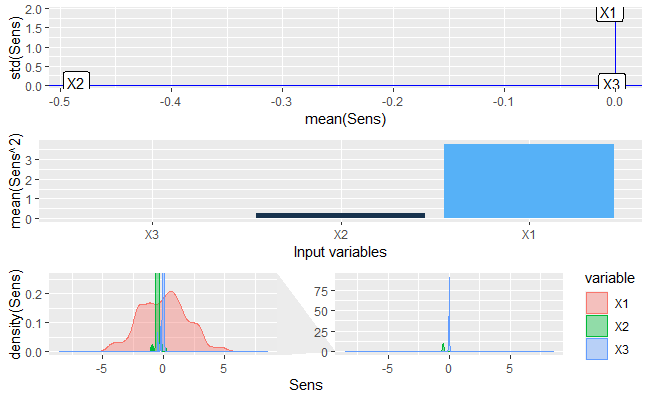
These plots can be obtained using the \codeSensitivityPlots() function and a ‘\codeSensMLP’ object calculated using \codeSensAnalysisMLP(). To obtain the plots of Figure 3: {CodeChunk} {CodeInput} R> SensitivityPlots(sens) Or they can be generated using the \codeplot() method of the ‘\codeSensMLP’ object: {CodeChunk} {CodeInput} R> plot(sens) In this case, the first plot of Figure 3 shows that \codeY has a negative linear relationship with \codeX2 ( and ), no relationship with \codeX3 ( and ) and a non-linear relationship with \codeX1 ( different from ). The second plot shows that \codeX3 barely affects the response variable, being \codeX1 and \codeX2 the inputs with most effect on the output.
3.4 Visualizing Neural Network Sensitivity over time
A common application of neural networks is time series forecasting. Analyzing how sensitivities evolve over time can provide a better understanding of the effect of explanatory variables on the output variables.
SensTimePlot() returns a sequence plot of the raw sensitivities calculated by the function \codeSensAnalysisMLP(). The x-axis is related to a \codenumeric or \codePosixct/\codePosixlt variable containing the time information of each sample. The y-axis is related to the sensitivities of the output with regard to each input.
In order to show how this function can be used, the \codeDAILY_DEMAND_TR dataset is used to create a model of class ‘\codetrain’ from \pkgcaret package (Kuhn et al. 2020). This dataset is similar to the \codeelecdaily dataset from \pkgfpp2 R package (Hyndman 2018). However, \codeDAILY_DEMAND_TR contains almost five years of daily data (\codeelecdaily only one year), which makes it more suitable for training a neural network. It is composed of the following variables:
- •
DATE: date of the sample, one per day from July, 2nd 2007 to November, 30th 2012.
- •
TEMP: mean daily temperature in ºC in Madrid, Spain.
- •
WD: working day, continuous parameter which represents the effect on the daily consumption of electricity as a percentage of the expected electricity demand of that day with regard to the demand of the reference day of the same week Moral-Carcedo and Vicéns-Otero 2005. In this case, Wednesday is the reference day (WD).
- •
DEM: total daily electricity demand in GWh for Madrid, Spain.

The following code creates the plot in Figure 4: {CodeChunk} {CodeInput} R> library("ggplot2") R> ggplot(DAILY_DEMAND_TR) + geom_point(aes(x = TEMP, y = DEM)) Figure 4 shows the relationship between the electricity demand and the temperature. A non-linear effect can be observed, where the demand increases for low temperatures (due to heating systems) and for high temperatures (due to air conditioners).

The following code scales the data, create a \codetrain neural network model and apply the \codeSensTimePlot() function to two years of the data: {CodeChunk} {CodeInput} R> DAILY_DEMAND_TR[,4] <- DAILY_DEMAND_TR[,4]/10 R> DAILY_DEMAND_TR[,2] <- DAILY_DEMAND_TR[,2]/100 R> library("caret") R> set.seed(150) R> mod2 <- train(form = DEM TEMP + WD, data = DAILY_DEMAND_TR, + method = "nnet", linout = TRUE, maxit = 250, metric = "RMSE", + tuneGrid = data.frame(size = 5, decay = 0.1), + preProcess = c("center","scale"), trControl = trainControl()) R> SensTimePlot(mod2, DAILY_DEMAND_TR[1:(365*2),], output_name = "DEM", + date.var = DAILY_DEMAND_TR[1:(365*2),1], facet = TRUE) Figure 5 shows that the temperature variable has a seasonal effect on the response variable. In summer, the temperature is higher and cooling systems demand more electricity, therefore the demand is directly proportional to the temperature. In winter, the temperature is lower and heating systems demand more electricity, hence the demand is inversely proportional to the temperature. The sensitivity of the output with regard to \codeWD has also a seasonal effect, with higher variance in winter than in summer and greater sensitivity in weekends. Figure 5 can also be generated using the \codeplot() method of a ‘\codeSensMLP’ object: {CodeChunk} {CodeInput} R> sens2 <- SensAnalysisMLP(mod2, trData = DAILY_DEMAND_TR[1:(365*2),], + output_name = "DEM", plot = FALSE) R> plot(sens2, plotType = "time", facet = TRUE, + date.var = DAILY_DEMAND_TR[1:(365*2),1])
3.5 Visualizing the Neural Network Sensitivity relation as a function of the input values
Sometimes it is useful to know how the value of the input variables affects the sensitivity of the response variables. The \codeSensFeaturePlot() function produces a violin plot to show the probability density of the output sensitivities with regard to each input. It also plots a jitter strip chart for each input, where the width of the jitter is controlled by the density distribution of the data (Pedersen and RStudio 2019). The color of the points is proportional to the value of each input variable, which display whether the relation of the output with the input is relatively constant within a range of input values.
The following code produce the plot of Figure 6: {CodeChunk} {CodeInput} R> SensFeaturePlot(mod2, fdata = DAILY_DEMAND_TR[1:(365*2),])
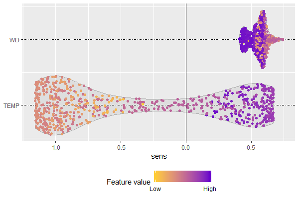
It can also be generated using the \codeplot() method of a ‘\codeSensMLP’ object: {CodeChunk} {CodeInput} R> plot(sens2, plotType = "features") In accordance with the information extracted from Figure 5, Figure 6 shows that the sensitivity of the output with regard to the temperature is negative when the temperature is low and positive when the temperature is high. It also shows that the sensitivity of the output with regard to \codeWD is higher in the weekends (lower values of \codeWD).
3.6 Extending package functionalities to other MLP models
The current version of \pkgNeuralSens package (version 1.0.0), includes methods of \codeSensAnalysisMLP() function for ‘\codenn’ (\pkgneuralnet), ‘\codennet’ (\pkgnnet), ‘\codeH2ORegressionModel’ and ‘\codeH2OMultinomialModel’ (\pkgh2o), ‘\codemlp’ (\pkgRSNNS), ‘\codelist’ (\pkgneural), ‘\codennetar’ (\pkgforecast) and ‘\codetrain’ (\pkgcaret) (only if the object inherits the class attribute from another of the available packages). Additionally, a ‘\codenumeric’ method is available to perform sensitivity analysis of a new neural network model using only the weights of the model, its neural structure, and the activation function of the layers and their derivatives. The first information that must be extracted from the model are the weights of the connections between layers. These weights must be passed to the first argument of the \codeSensAnalysisMLP() function as a ‘\codenumeric’ ‘\codevector’, concatenating the weights of the layers in order from the first hidden layer () to the output layer (). The bias weight should be added to the vector before the weights of the same layer, following the equation below:
| (15) |
If the model has no bias, the bias weights must be set to 0 ().
The second information is the neural structure of the model. The structure of the model must be passed to the \codemlpstr argument as a ‘\codenumeric’ ‘\codevector’ equal in length to the number of layers in the network. Each number specifies the number of neurons in each layer, starting with the input layer and ending with the output layer:
The last information that must be provided are the activation functions of each layer and their derivatives. If the activation function of a layer is one of those provided by the package (shown in Table 1), the function can be specified using its name. If the activation function is not one of those provided in the package, it should be passed as a function. The same applies to the derivative of the activation function. The activation function of a layer and its derivative must meet the following conditions:
- •
must return a ‘\codevector’ with the same length as . The activation function of each neuron may be different, as long as this condition is met:
(16) - •
must return a square ‘\codematrix’ with the derivative of with regard to each component of :
(17)
Examples of how to use the \codeSensAnalysisMLP() function with new packages can be found in Appendix A.
3.7 Effect of network structure and training conditions
An important advantage of sensitivity analysis based on partial derivatives is the robustness of the analysis results regardless of the model’s neural structure. Other methods such as Olden rely heavily on the neural structure and the initial starting weights. A similar analysis to the one performed on \codeolden() in Beck 2018 has been performed on the \codeSensAnalysisMLP() function. To observe the effect of the neural structure on the sensitivity metrics, these metrics have been calculated for models with 1, 10 and 20 neurons in the hidden layer. For each neuron level, 50 models with different random initial weights are trained. If the neural structure and the initial starting weights have no effect on the sensitivity metrics, these metrics should be the same for all the models. \codesimdata dataset is used to train the models.
Figure 7 shows the mean value of the sensitivity metrics from the 50 models for each neural structure. It also shows the minimum and maximum value of the metric to display the effect of the neural structure and the initial weights values. An important conclusion that can be derived from Figure 7 is that with enough neurons in the hidden layer, i.e., if the model can predict the output with enough precision; variance of sensitivity metrics is negligible compared to the value of the metric.

4 Further examples and comparison with other methods
This section contains several examples in which the functions of the \pkgNeuralSens package are compared with similar functions from other \proglangR packages. Section 4.1 trains an MLP for classification to compare \codeSensAnalysisMLP() with \codeolden(), \codegarson() (Beck 2018) and \codeplot_explanations() (Pedersen and Benesty 2019). Section 4.2 trains an MLP for regression to compare \codeSensAnalysisMLP() and \codeSensFeaturePlot() with \codelekprofile() (Beck 2018) and \codepartial() (Greenwell 2017).
Topics such as data pre-processing or network architecture should be considered before model development. Discussions about these ideas have been already held (Cannas et al. 2006, Amasyali and El-Gohary 2018, Maier and Dandy 2000, Lek et al. 1996) and are beyond the scope of this paper.
4.1 Multilayer perceptron for classification
In this example a multilayer perceptron is trained using the well-known \codeiris dataset included in R. Figure 8 shows two scatterplots comparing the petal-related and sepal-related variables of the flowers in the dataset. It can be seen that \codesetosa species have a smaller petal size than the other two species and a shorter sepal. It also shows that \codevirginica and \codeversicolor species have a similar sepal size, but the latter has a slightly smaller petal size.


The \codetrain() function from the \pkgcaret package creates a new neural network model to predict the species of each flowers based on petal and sepal dimensions. {CodeChunk} {CodeInput} R> set.seed(150) R> mod3 <- caret::train(Species ., data = iris, preProcess = c("center", + "scale"), method = "nnet", linout = TRUE, trControl = trainControl(), + tuneGrid = data.frame(size = 5, decay = 0.1), metric = "Accuracy") \codeSensAnalysisMLP() function calculates the sensitivities of the model, providing information of the relationships between each output class and each input variable. {CodeChunk} {CodeInput} R> sens4 <- SensAnalysisMLP(mod3) R> summary(sens4) {CodeOutput} Sensitivity analysis of 4-5-3 MLP network.
Sensitivity measures of each output: versicolor mean std meanSensSQ Sepal.Length 0.035833076 0.02252307 0.04228375 Sepal.Width -0.002101449 0.03925762 0.03918294 Petal.Length -0.099221391 0.17568963 0.20126091 Petal.Width -0.093949654 0.16300239 0.18766775
S_ik^sq
4.2 Multilayer perceptron for regression
The \codeBoston dataset from the \pkgMASS (Ripley et al. 2019) package is used to train an \codennet (Venables and Ripley 2002) model. This dataset contains information collected by the U.S. Census Service on housing in the suburbs of Boston (run \code?MASS::Boston to obtain more information about the dataset).
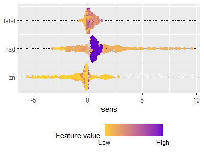
The objective of the model is to predict the nitric oxides concentration (parts per 10 million), stored in the \codenox variable. The input variables of the model are \codezn (proportion of residential land zoned for lots over 25,000 sq.ft.), \coderad (index of accessibility to radial highways) and \codelstat (lower status of the population (percent)). \codescale() function standardizes the input variables. \codeSensFeaturePlot(), \codeSensAnalysisMLP(), \codelekprofile() (\pkgNeuralNetTools Beck 2018) and \codepdp() (\pkgpdp Greenwell 2017) functions analyze the relationships of the output with regard to the inputs. {CodeChunk} {CodeInput} R> data("Boston", package = "MASS") R> Boston <- as.data.frame(scale(Boston[,c("zn","rad","lstat","nox")])) R> set.seed(150) R> mod4 <- nnet::nnet(nox ., data = Boston, size = 15, decay = 0.1, + maxit = 150) R> lekprofile(mod4, group_vals = 6) R> lekprofile(mod4, group_vals = 6, group_show = TRUE) R> library("pdp") R> pdps <- list() R> for (i in 1:3) + pdps[[i]] <- autoplot(partial(mod4, pred.var = names(Boston)[i], + train = Boston, ice = TRUE), train = Boston, + center = TRUE, alpha = 0.2, rug = TRUE) + + theme_bw() + ylab("nox") + R> gridExtra::grid.arrange(grobs = pdps, nrow = 1) R> SensFeaturePlot(mod4, fdata = Boston, output_name = "nox") R> SensAnalysisMLP(mod4, trData = Boston, output_name = "nox")



Figures 11(a) and 11(b) display the results of Lek’s profile method from the \pkgNeuralNetTools package. To prevent the analysis of non-representative scenarios in the input dataset, a k-means clustering with 6 clusters has been applied to the dataset. Each subplot in Figure 11(a) shows the evolution of the output variable when varying the input variable of interest across a range of values corresponding to the center of the k-means clusters. The other inputs remain constant in their values in the center of each k-means cluster. Figure 11(b) shows the value of the input variables at each of the cluster centers.
Figure 11(c) shows the partial dependence plots (pdp) and Individual Conditional Expectaction (ICE) plots of \codemod4 output with regard to each input variable. An ICE curve is calculated by maintaining the input variable of interest at a value , where is the value of in the row of the dataset, and varying all other inputs across their values in the dataset. For a given dataset with samples, there would be ICE curves for each input variable. The PDP curve can be calculated as the mean of these ICE curves. PDP shows the marginal effect a given input variable has on the response variable of the neural network model, averaging the effects of the rest of the input variables.
Calculating all ICE curves shows how the output variable change in the entire input space of the dataset. This comes at a large computational cost, since the number of curves that must be calculated are directly proportional to the number of samples and number of input variables. The computational time can be reduced by calculating only the PDP or a reduced number of ICE curves, but in that case some important scenarios might be ignored.
SensFeaturePlot() function performs an analysis similar to Lek’s and \codepdp by plotting the sensitivity of the output with regard to the input colored proportionally to the value of the input variable. On the one hand, \codelekprofile() function indicates that \codelstat and \coderad have a direct relationship with the output and \codezn has an inverse relationship with the output. Figure 11(a) also suggests that all the input variables have a non-linear relationship with the output. On the other hand, Figure 11(d) shows that the sensitivity of the output has an approximately linear relationship with \codezn, and a non-linear relationship with the other two inputs. In this case, the \codelekprofile() function gives more information about the model, but it can be difficult to understand how the value of the input variables in each group affects the output variable.
SensAnalysisMLP() can be used to obtain more information on variable importance and relationships between variables. In this case, the \coderad variable affects the output the most, information which can be difficult to extract from the other functions.
4.3 Computational cost
As the size of neural network models increase exponentially to solve more complex tasks, performing a sensitivity analysis of a model could become an intensive computational task. Sensitivity analysis using partial derivatives requires matrix calcules where the size of the matrixes is directly proportional to the size of the hidden layers. As the number of neurons in hidden layers increase, the time to perform these calculations grows rapidly.
A comparison of how much time is required by a sensitivity analysis using the different methods included in Section 4 has been performed. This comparison has been carried out using the \codeYearPredictionMSD dataset. This dataset consists of 90 input variables and 515345 samples. The authors propose to measure the computational time when varying the number of input variables, the number of samples and the size of the hidden layer of a single hidden layer MLP model.


This analysis has been performed on a computer with the following specs: processor Intel(R) Core(TM) i7-8700 @3.20 GHz, 32 GB of RAM memory, R version 3.6.3 (2020-02-29), platform x86_64-w64-mingw32/x64 (64-bit) and running under Windows 10 x64 (build 18362).
Figure 12 shows the computational time of each function varying the number of training samples, the number of input variables and the number of neurons in the hidden layer. Some conclusions can be reached from this figure:
- •
The fastest functions are the \codeolden() and \codegarson() functions from the \pkgNeuralNetTools package, because they only perform a sum of the weight matrices of the model. As it does not depend of the number of samples, the computational time is directly proportional to the size of the neural network layers (input and hidden layers).
- •
\code
lekprofile() from \pkgNeuralNetTools and \codeSensAnalysisMLP() from \pkgNeuralSens need of the similar computational times.h \codeSensAnalysisMLP() is affected byFthe number of neurons in the hidden layer and the number of samples, as the size of the matrixes increases with the number of neurons and the number of matrixes multiplication increase with the number of samples. \codelekprofile() is more affected by the number of input variables, because the number of curves to be created increase with the number of input variables. However, due to the fact that it uses only a fixed number of scenarios it does not depend on the number of samples. Since the number of neurons in the hidden layer barely affects the computational time to predict the output variable in each scenario, this parameter does not affect the computational time of lekprofile.
- •
The slowest function is the \codepartial() function from the \pkgpdp package when calculating all ICE curves. Calculating all ICE curves instead of only the pdp curves adds a noticeable amount of computational time. However, if the form of the ICE curves is not constant throughout the samples of the dataset (as in Figure 11(c)), showing only the pdp curve gives misleading information as the form of the pdp curve does not resemble all the ICE curves. The computational time for \codepartial() is directly proportional to the number of samples and the number of input variables, because the number of curves to be calculated increase exponentially as these parameters increase.
In addition to these conclusions, it must be mentioned that this analysis has been performed using a model with only one output variable. If there were several output variables, to obtain analogous information as \codeSensAnalysisMLP() the other functions must be called once for each output. Because of this, the computational time of all the functions except \codeSensAnalysisMLP() must be multiplied by the number of output variables of the model in order to obtain an approximate idea of the computational time they require.
5 Conclusions
The \pkgNeuralSens package provides functions to extract information from a fitted feed-forward MLP neural network in \proglangR. These functions can be used to obtain the partial derivatives of the neural network response variables with regard to the input variables and to generate plots to obtain different information on the network using these partial derivatives. Methods are available for the next CRAN packages: ‘\codenn’ (\pkgneuralnet), ‘\codennet’ (\pkgnnet), ‘\codemlp’ (\pkgRSNNS), ‘\codeH2ORegressionModel’ and ‘\codeH2OMultinomialModel’ (\pkgh2o), ‘\codelist’ (\pkgneural), ‘\codennetar’ (\pkgforecast) and ‘\codetrain’ (\pkgcaret) (only if the object inherits the class attribute from another package). An additional method for class ‘\codenumeric’ is available to use with the basic information of the model (weights, structure and activation functions of the neurons).
The main objective of the package is to help the user to understand how the neural network uses the inputs to predict the output. This information may be useful for simplifying the neural network structure by eliminating the inputs which have no effect on the output. It could also provide a deeper understanding on the problem and the relationship among variables. \pkgNeuralSens is another tool among several other methods for exploratory data analysis and model evaluation, and it can be used with other packages (Beck 2018, Greenwell 2017) to obtain more information on the neural network model. Nevertheless, it must be noted that sensitivity analysis using partial derivatives provides information about variable relationships such as pdp or ICE plots significantly faster. Moreover, it also provides variable importance measures like Garson’s or Olden’s methods and these measures are independent of the neural structure and training conditions of the model as long as it predicts the output with enough precision.
Improving the information given by these methods will have value for exploratory data-analysis and characterization of relationships among variables. Future versions of the package may include additional functionalities as:
- •
Parallelizing the sensitivity calculations when workers registered to work in parallel are detected.
- •
Calculating the sensitivities of the output variables with regard to the output of hidden neurons, in order to obtain the importance of each hidden neuron and helping to select the optimal network structure.
- •
Calculating the sensitivities of other neural network models such as Probabilistic Radial Basis Function Network (PRBFN) or Recurrent Neural Network (RNN).
- •
Calculating the second order partial derivatives of an MLP model to analyze the effect of interactions between two input variables.
- •
Develop a statistic to determine if the relationship between the output and input is linear.
References
- Allaire and Chollet (2020) Allaire J, Chollet F (2020). keras: R Interface to ’Keras’. R package version 2.2.5.0, URL https://keras.rstudio.com.
- Allaire and Tang (2020) Allaire J, Tang Y (2020). tensorflow: R Interface to ’TensorFlow’. R package version 2.0.0, URL https://github.com/rstudio/tensorflow.
- Amasyali and El-Gohary (2018) Amasyali K, El-Gohary NM (2018). “A Review of Data-Driven Building Energy Consumption Prediction Studies.” Renewable and Sustainable Energy Reviews, 81, 1192–1205. ISSN 1364-0321. https://doi.org/10.1016/j.rser.2017.04.095.
- Beck (2018) Beck MW (2018). “\pkgNeuralNetTools : Visualization and Analysis Tools for Neural Networks.” Journal of Statistical Software, 85(11). ISSN 1548-7660. 10.18637/jss.v085.i11. URL http://www.jstatsoft.org/v85/i11/.
- Bergmeir and Benítez (2012) Bergmeir C, Benítez JM (2012). “Neural Networks in \proglangR Using the Stuttgart Neural Network Simulator: \pkgRSNNS.” Journal of Statistical Software, 46(7), 1–26. URL http://www.jstatsoft.org/v46/i07/.
- Butler et al. (2018) Butler KT, Davies DW, Cartwright H, Isayev O, Walsh A (2018). “Machine Learning for Molecular and Materials Science.” Nature, 559(7715), 547–555. ISSN 0028-0836, 1476-4687. 10.1038/s41586-018-0337-2.
- Cannas et al. (2006) Cannas B, Fanni A, See L, Sias G (2006). “Data Preprocessing for River Flow Forecasting Using Neural Networks: Wavelet Transforms and Data Partitioning.” Elsevier, 31, 1164–1171. https://doi.org/10.1016/j.pce.2006.03.020.
- Cannon (2017) Cannon AJ (2017). monmlp: Multi-Layer Perceptron Neural Network with Optional Monotonicity Constraints. R package version 1.1.5, URL https://CRAN.R-project.org/package=monmlp.
- Chambers and Hastie (1992) Chambers JM, Hastie TJ (1992). Classes and Methods: Object-Oriented Programming in S. URL https://stat.ethz.ch/R-manual/R-devel/library/methods/html/Methods_for_S3.html.
- Cybenko (1989) Cybenko G (1989). “Approximation by Superpositions of a Sigmoidal Function.” Mathematics of Control, Signals and Systems, 2(4), 303–314. ISSN 1435-568X. 10.1007/BF02551274.
- Dimopoulos et al. (1995) Dimopoulos I, Bourret P, Lek S (1995). “Use of Some Sensitivity Criteria for Choosing Networks with Good Generalization Ability.” Neural Processing Letters, 2, 1–4. 10.1007/BF02309007.
- Dimopoulos et al. (1999) Dimopoulos I, Chronopoulos J, Chronopoulou-Sereli A, Lek S (1999). “Neural Network Models to Study Relationships Between Lead Concentration in Grasses and Permanent Urban Descriptors in Athens City (Greece).” Ecological Modelling, 120(2-3), 157–165. ISSN 03043800. 10.1016/S0304-3800(99)00099-X.
- Engelbrecht et al. (1995) Engelbrecht AP, Cloete I, Zurada JM (1995). “Determining the Significance of Input Parameters Using Sensitivity Analysis.” In G Goos, J Hartmanis, J Leeuwen, J Mira, F Sandoval (eds.), From Natural to Artificial Neural Computation, volume 930, pp. 382–388. Springer-Verlag, Berlin, Heidelberg. ISBN 978-3-540-59497-0 978-3-540-49288-7. 10.1007/3-540-59497-3_199.
- Friedman (2001) Friedman JH (2001). “Greedy Function Approximation: A Gradient Boosting Machine.” Annals of Statistics, 29(5), 1189–1232. 10.1214/aos/1013203451.
- Fritsch et al. (2019) Fritsch S, Guenther F, Wright MN (2019). “\pkgneuralnet: Training of Neural Networks.” \proglangR package version 1.44.2, URL https://CRAN.R-project.org/package=neuralnet.
- Garson (1991) Garson GD (1991). “Interpreting Neural-Network Connection Weights.” AI Expert, 6(4), 46–51. ISSN 0888-3785.
- Gevrey et al. (2003) Gevrey M, Dimopoulos I, Lek S (2003). “Review and Comparison of Methods to Study the Contribution of Variables in Artificial Neural Networks Models.” Ecological Modelling, 160, 249–264. 10.1016/S0304-3800(02)00257-0.
- Goldstein et al. (2015) Goldstein A, Kapelner A, Bleich J, Pitkin E (2015). “Peeking Inside the Black Box: Visualizing Statistical Learning With Plots of Individual Conditional Expectation.” Journal of Computational and Graphical Statistics, 24(1), 44–65. 10.1080/10618600.2014.907095. URL https://doi.org/10.1080/10618600.2014.907095.
- Greenwell (2017) Greenwell BM (2017). “\pkgpdp: An \proglangR Package for Constructing Partial Dependence Plots.” The \proglangR Journal, 9(1), 421–436. URL https://journal.r-project.org/archive/2017/RJ-2017-016/index.html.
- Hastie et al. (2001) Hastie T, Tibshirani R, Friedman J (2001). The Elements of Statistical Learning. Springer Series in Statistics. Springer-Verlag, New York.
- Hornik (1991) Hornik K (1991). “Approximation Capabilities of Multilayer Feedforward Networks.” Neural Networks, 4(2), 251–257. ISSN 0893-6080. 10.1016/0893-6080(91)90009-T.
- Hornik et al. (1989) Hornik K, Stinchcombe M, White H (1989). “Multilayer Feedforward Networks are Universal Approximators.” Neural Networks, 2(5), 359–366. ISSN 08936080. 10.1016/0893-6080(89)90020-8.
- Hyndman (2018) Hyndman R (2018). \pkgfpp2: Data for "Forecasting: Principles and Practice" (2nd Edition). \proglangR package version 2.3, URL https://CRAN.R-project.org/package=fpp2.
- Hyndman and Khandakar (2008) Hyndman RJ, Khandakar Y (2008). “Automatic Time Series Forecasting: the \pkgforecast Package for \proglangR.” Journal of Statistical Software, 26(3), 1–22. URL http://www.jstatsoft.org/article/view/v027i03.
- Kuhn et al. (2020) Kuhn M, Wing J, Weston S, Williams A, Keefer C, Engelhardt A, Cooper T, Mayer Z, Kenkel B, the \proglangR Core Team, Benesty M, Lescarbeau R, Ziem A, Scrucca L, Tang Y, Candan C, Hunt T (2020). “\pkgcaret: Classification and Regression Training.” \proglangR package version 6.0-85, URL https://CRAN.R-project.org/package=caret.
- LeDell et al. (2019) LeDell E, Gill N, Aiello S, Fu A, Candel A, Click C, Kraljevic T, Nykodym T, Aboyoun P, Kurka M, Malohlava M (2019). “\pkgh2o: \proglangR Interface for ’H2O’.” \proglangR package version 3.26.0.2, URL https://CRAN.R-project.org/package=h2o.
- Lek et al. (1996) Lek S, Delacoste M, Baran P, Dimopoulos I, Lauga J, Aulagnier S (1996). “Application of Neural Networks to Modeling Nonlinear Relationships in Ecology.” Ecological Modelling, 90, 39–52. 10.1016/0304-3800(95)00142-5.
- Maier and Dandy (2000) Maier HR, Dandy GC (2000). “Neural Networks for the Prediction and Forecasting of Water Resources Variables: A Review of Modelling Issues and Applications.” Environmental Modelling And Software, 15(1), 101–124. ISSN 1364-8152. https://doi.org/10.1016/S1364-8152(99)00007-9.
- McCulloch and Pitts (1943) McCulloch WS, Pitts W (1943). “A Logical Calculus of the Ideas Immanent in Nervous Activity.” The bulletin of mathematical biophysics, 5(4), 115–133. ISSN 1522-9602. 10.1007/BF02478259.
- Moral-Carcedo and Vicéns-Otero (2005) Moral-Carcedo J, Vicéns-Otero J (2005). “Modelling the Non-Linear Response of Spanish Electricity Demand to Temperature Variations.” Energy Economics, 27(3), 477–494. ISSN 01409883. 10.1016/j.eneco.2005.01.003.
- Mosavi et al. (2019) Mosavi A, Salimi M, Faizollahzadeh Ardabili S, Rabczuk T, Shamshirband S, Varkonyi-Koczy AR (2019). “State of the Art of Machine Learning Models in Energy Systems, a Systematic Review.” Energies, 12(7), 1301. ISSN 1996-1073. 10.3390/en12071301.
- Muñoz and Czernichow (1998) Muñoz A, Czernichow T (1998). “Variable Selection Using Feedforward and Recurrent Neural Networks.” Engineering Intelligent Systems for Electrical Engineering and Communications, 6(2), 102.
- Nagy (2014) Nagy A (2014). “\pkgneural: Neural Networks.” \proglangR package version 1.4.2.2, URL https://CRAN.R-project.org/package=neural.
- Olden et al. (2004) Olden JD, Joy MK, Death RG (2004). “An Accurate Comparison of Methods for Quantifying Variable Importance in Artificial Neural Networks Using Simulated Data.” Ecological Modelling, 178(3-4), 389–397. ISSN 03043800. 10.1016/j.ecolmodel.2004.03.013.
- Pedersen and Benesty (2019) Pedersen TL, Benesty M (2019). \pkglime: Local Interpretable Model-Agnostic Explanations. \proglangR package version 0.5.1, URL https://CRAN.R-project.org/package=lime.
- Pedersen and RStudio (2019) Pedersen TL, RStudio (2019). “\pkgggforce: Accelerating ’\pkgggplot2’.” \proglangR package version 0.3.1, URL https://CRAN.R-project.org/package=ggforce.
- Philip Chen and Zhang (2014) Philip Chen C, Zhang CY (2014). “Data-Intensive Applications, Challenges, Techniques and Technologies: A Survey on Big Data.” Information Sciences, 275, 314–347. ISSN 00200255. 10.1016/j.ins.2014.01.015. URL https://linkinghub.elsevier.com/retrieve/pii/S0020025514000346.
- Pizarroso et al. (2019) Pizarroso J, Portela J, Muñoz A (2019). “\pkgNeuralSens: Sensitivity Analysis of Neural Networks.” \proglangR package version 0.2.0, URL https://CRAN.R-project.org/package=NeuralSens.
- \proglangR Core Team (2017) \proglangR Core Team (2017). “\proglangR: A Language and Environment for Statistical Computing.” URL https://www.R-project.org/.
- Ribeiro et al. (2016) Ribeiro MT, Singh S, Guestrin C (2016). “"Why Should I Trust You?": Explaining the Predictions of Any Classifier.” In Proceedings of the 22Nd ACM SIGKDD International Conference on Knowledge Discovery and Data Mining, KDD ’16, pp. 1135–1144. ACM, New York, NY, USA. ISBN 978-1-4503-4232-2. 10.1145/2939672.2939778. Event-place: San Francisco, California, USA.
- Ripley et al. (2019) Ripley B, Venables B, Bates DM, Hornik K, Gebhardt A, Firth D, ca (2019). “\pkgMASS: Support Functions and Datasets for Venables and Ripley’s \pkgMASS.” URL https://CRAN.R-project.org/package=MASS.
- Rojas (1996) Rojas R (1996). “Fast Learning Algorithms.” In Neural Networks, pp. 183–225. Springer-Verlag, Berlin, Heidelberg. ISBN 978-3-540-60505-8 978-3-642-61068-4. 10.1007/978-3-642-61068-4_8.
- Rumelhart et al. (1986) Rumelhart DE, Hinton GE, Williams RJ (1986). “Learning Representations by Back-Propagating Errors.” Nature, 323, 533–536.
- Scardi and Harding (1999) Scardi M, Harding LW (1999). “Developing an Empirical Model of Phytoplankton Primary Production: A Neural Network Case Study.” Ecological Modelling, 120(2-3), 213–223. ISSN 03043800. 10.1016/S0304-3800(99)00103-9.
- Smalley (2017) Smalley E (2017). “AI-Powered Drug Discovery Captures Pharma Interest.” Nature Biotechnology, 35(7), 604–605. ISSN 1087-0156, 1546-1696. 10.1038/nbt0717-604.
- Sun et al. (2018) Sun Z, Sun L, Strang KD (2018). “Big Data Analytics Services for Enhancing Business Intelligence.” Journal of Computer Information Systems, 58(2), 162–169. ISSN 0887-4417, 2380-2057. 10.1080/08874417.2016.1220239.
- Valduriez et al. (2018) Valduriez P, Mattoso M, Akbarinia R, Borges H, Camata JJ, Coutinho A, Gaspar D, Lemus NM, Liu J, Lustosa H, Masseglia F, Silva FN, Sousa VS, Souza R, Ocaña KACS, Ogasawara ES, de Oliveira D, Pacitti E, Porto F, Shasha D (2018). “Scientific Data Analysis Using Data-Intensive Scalable Computing: The SciDISC Project.” In LADaS@VLDB.
- Venables and Ripley (2002) Venables WN, Ripley BD (2002). Modern Applied Statistics with \proglangS. Fourth edition. Springer-Verlag, New York. ISBN 0-387-95457-0, URL http://www.stats.ox.ac.uk/pub/MASS4.
- Vu et al. (2018) Vu MAT, Adalı T, Ba D, Buzsáki G, Carlson D, Heller K, Liston C, Rudin C, Sohal VS, Widge AS, Mayberg HS, Sapiro G, Dzirasa K (2018). “A Shared Vision for Machine Learning in Neuroscience.” The Journal of Neuroscience, 38(7), 1601–1607. ISSN 0270-6474, 1529-2401. 10.1523/JNEUROSCI.0508-17.2018.
- White and Racine (2001) White H, Racine J (2001). “Statistical Inference, the Bootstrap, and Neural-Network Modeling with Application to Foreign Exchange Rates.” IEEE Transactions on Neural Networks, 12(4), 657–673. ISSN 10459227. 10.1109/72.935080.
- Wickham (2016) Wickham H (2016). \pkgggplot2: Elegant Graphics for Data Analysis. Springer-Verlag, New York. ISBN 978-3-319-24277-4. URL https://ggplot2.tidyverse.org.
- Xu and Tian (2015) Xu D, Tian Y (2015). “A Comprehensive Survey of Clustering Algorithms.” Annals of Data Science, 2. 10.1007/s40745-015-0040-1.
- Yeh and Cheng (2010) Yeh IC, Cheng WL (2010). “First and Second Order Sensitivity Analysis of MLP.” Neurocomputing, 73(10-12), 2225–2233. ISSN 09252312. 10.1016/j.neucom.2010.01.011. URL https://linkinghub.elsevier.com/retrieve/pii/S0925231210000639.
- Özesmi and Özesmi (1999) Özesmi SL, Özesmi U (1999). “An Artificial Neural Network Approach to Spatial Habitat Modelling with Interspecific Interaction.” Ecological Modelling, 116(1), 15–31. ISSN 03043800. 10.1016/S0304-3800(98)00149-5.
- Zhang et al. (2018) Zhang Z, Beck MW, Winkler DA, Huang B, Sibanda W, Goyal H (2018). “Opening the Black Box of Neural Networks: Methods for Interpreting Neural Network Models in Clinical Applications.” Annals of Translational Medicine, 6(11). ISSN 2305-5839. 10.21037/atm.2018.05.32.
- Zurada et al. (1994) Zurada JM, Malinowski A, Cloete I (1994). “Sensitivity Analysis for Minimization of Input Data Dimension for Feedforward Neural Network.” In Proceedings of IEEE International Symposium on Circuits and Systems - ISCAS ’94, volume 6, pp. 447–450. IEEE, London, UK. ISBN 978-0-7803-1915-8. 10.1109/ISCAS.1994.409622.
Appendix A Examples of \codeSensAnalysisMLP() ‘\codenumeric’ method
The \proglangR packages \pkgmonmlp (Cannon 2017) and \pkgtensorflow (Allaire and Tang 2020) is used in this section to illustrate how the ‘\codenumeric’ method of \codeSensAnalysisMLP() function can be applied to new models. The \codesimdata dataset described in section 3.2 is used to train the MLP models in this appendix. {CodeChunk} {CodeInput} R> library("monmlp") R> set.seed(150) R> monmlp_model <- monmlp.fit(x = data.matrix(simdata[,1:3]), + y = data.matrix(simdata[,4]), hidden1 = 5, iter.max = 250, + silent = TRUE) The weights of the model are extracted and ordered as described in (15): {CodeChunk} {CodeInput} R> W1 <- rbind(monmlp_model[[1]]W1[1:3,]) R> W2 <- c(monmlp_model[[1]]W2[1:5,]) R> wts <- c(as.vector(W1), as.vector(W2)) The activation functions of the hidden and output layers and their derivatives are provided in the ‘\codeTh’, ‘\codeTo’, ‘\codeTh.prime’ and ‘\codeTo.prime’ attribute of the model respectively. However, the derivative functions does not meet the condition of returning a square ‘\codematrix’ so it must be modified before using \codeSensAnalysisMLP(): {CodeChunk} {CodeInput} R> Actfunc <- c("linear", attr(monmlp_model, "Th"), + attr(monmlp_model, "To")) R> Deractfunc <- c("linear", + function(v) diag(attr(monmlp_model, "Th.prime")(v)), + function(v) diag(attr(monmlp_model, "To.prime")(v))) The last information that must be passed to \codeSensAnalysisMLP() is the neural structure: {CodeChunk} {CodeInput} R> mlpstruct <- c(3,5,1) Since \codemonmlp.fit() automatically scales the variables when training the model, the input variables must be scaled before calculating the sensitivities. {CodeChunk} {CodeInput} R> x <- data.matrix(simdata[,1:3]) R> x.center <- attr(monmlp_model, "x.center") R> x.scale <- attr(monmlp_model, "x.scale") R> x <- sweep(x, 2, x.center, "-") R> x <- sweep(x, 2, x.scale, "/") R> x <- cbind(data.frame(x),Y = simdata[,4]) Once all the information has been prepared, the ‘\codenumeric’ method of \codeSensAnalysisMLP() can be used to perform a sensitivity analysis of the model: {CodeChunk} {CodeInput} R> sens_monmlp <- SensAnalysisMLP(wts, trData = x, mlpstr = mlpstruct, + coefnames = c("X1", "X2", "X3"), output_name = "Y", + actfunc = Actfunc, deractfunc = Deractfunc, plot = FALSE) R> summary(sens_monmlp) {CodeOutput} Sensitivity analysis of 3-5-1 MLP network.
Sensitivity measures of each output:
