Time integration of tree tensor networks
Abstract
Dynamical low-rank approximation by tree tensor networks is studied for the data-sparse approximation of large time-dependent data tensors and unknown solutions to tensor differential equations. A time integration method for tree tensor networks of prescribed tree rank is presented and analyzed. It extends the known projector-splitting integrators for dynamical low-rank approximation by matrices and rank-constrained Tucker tensors and is shown to inherit their favorable properties. The integrator is based on recursively applying the low-rank Tucker tensor integrator. In every time step, the integrator climbs up and down the tree: it uses a recursion that passes from the root to the leaves of the tree for the construction of initial value problems on subtree tensor networks using appropriate restrictions and prolongations, and another recursion that passes from the leaves to the root for the update of the factors in the tree tensor network. The integrator reproduces given time-dependent tree tensor networks of the specified tree rank exactly and is robust to the typical presence of small singular values in matricizations of the connection tensors, in contrast to standard integrators applied to the differential equations for the factors in the dynamical low-rank approximation by tree tensor networks.
keywords
Tree tensor network, tensor differential equation, dynamical low-rank approximation, time integratorAMS
15A69, 65L05, 65L20, 65L701 Introduction
For the approximate solution of the initial value problem for a (huge) system of differential equations for the tensor ,
| (1) |
we aim to construct in an approximation manifold of much smaller dimension, which in the present work will be chosen as a manifold of tree tensor networks of fixed tree rank. This shall provide a data-sparse computational approach to high-dimensional problems that cannot be treated by direct time integration because of both excessive memory requirements and computational cost.
A differential equation for is obtained by choosing the time derivative as that element in the tangent space for which
where the norm is chosen as the Euclidean norm of the vector of the tensor entries. In the quantum physics and chemistry literature, this approach is known as the Dirac–Frenkel time-dependent variational principle, named after work by Dirac in 1930 who used the approach in the context of what is nowadays known as the time-dependent Hartree–Fock method for the multi-particle time-dependent Schrödinger equation; see, e.g., [16, 17]. Equivalently, this minimum-defect condition can be stated as a Galerkin condition on the state-dependent approximation space ,
Using the orthogonal projection onto the tangent space , this can be reformulated as the (abstract) ordinary differential equation on ,
| (2) |
This equation needs to be solved numerically in an efficient and robust way. For fixed-rank matrix and tensor manifolds, the orthogonal projection turns out to be an alternating sum of subprojections, which reflects the multilinear structure of the problem. The explicit form of the tangent space projection in the low-rank matrix case as an alternating sum of three subprojections was derived in [14] and was used in [19] to derive a projector-splitting integrator for low-rank matrices, which efficiently updates an SVD-like low-rank factorization in every time step and which is robust to the typically arising small singular values that cause severe difficulties with standard integrators applied to the system of differential equations for the factors of the SVD-like decomposition of the low-rank matrices; see [12]. The projector-splitting integrator was extended to tensor trains / matrix product states in [20]; see also [10] for a description of the algorithm in a physical idiom. The projector-splitting integrator was extended to Tucker tensors of fixed multilinear rank in [18]. A reinterpretation was given in [21], in which the Tucker tensor integrator was rederived by recursively performing inexact substeps in the matrix projector-splitting integrator applied to matricizations of the tensor differential equation followed by retensorization. This interpretation made it possible to show that the Tucker integrator inherits the favorable robustness properties of the low-rank matrix projector-splitting integrator.
In the present paper we take up such a recursive approach to derive an integrator for general tree tensor networks, which is shown to be efficiently implementable (provided that the righthand side function can be efficiently evaluated on tree tensor networks in factorized form) and to inherit the robust convergence properties of the low-rank matrix, Tucker tensor and tensor train / matrix product state integrators shown previously in [12, 21]. The proposed integrator for tree tensor networks reduces to the well-proven projector-splitting integrators in the particular cases of Tucker tensors and tensor trains / matrix product states. We expect (but will not prove) that it can itself be interpreted as a projector-splitting integrator based on splitting the tangent space projection of the fixed-rank tree tensor network manifold.
For a special tree, this integrator (given in an ad hoc formulation) was already used in [5] for the Vlasov–Poisson equation of plasma physics. In that case, the tree is given by the separation of the position and velocity variables, which are further separated into their Cartesian coordinates. Very recently, this tree tensor network integrator (or very similar versions) was applied to problems of current interest in quantum physics in [3] and [13], studying multi-orbital Anderson impurity models and the dynamics in two-dimensional quantum lattices, respectively. None of these papers gives a systematic construction and numerical analysis of the integrator. This is the objective of the present paper.
In Section 2 we introduce notation and the formulation of tree tensor networks as multilevel-structured Tucker tensors and give basic properties, emphasizing orthonormal factorizations. The tree tensor network (TTN) is constructed from the basis matrices at the leaves and the connection tensors at the inner vertices of the tree in a multilinear recursion that passes from the leaves to the root of the tree.
In Section 3 we recall the algorithm of the Tucker tensor integrator of [21] and extend it to the case of several Tucker tensors with the same basis matrices. This extended Tucker integrator, which is nothing but the Tucker integrator for an extended Tucker tensor, is a basic building block of the integrator for tree tensor networks.
In Section 4, the main algorithmic section of this paper, we derive the recursive TTN integrator and discuss the basic algorithmic aspects. In every time step, the integrator uses a recursion that passes from the root to the leaves of the tree for the construction of initial value problems on subtree tensor networks using appropriate restrictions and prolongations, and another recursion that passes from the leaves to the root for the update of the factors in the tree tensor network. The integrator only solves low-dimensional matrix differential equations (of the dimension of the basis matrices at the leaves) and low-dimensional tensor differential equations (of the dimension of the connection tensors at the inner vertices of the tree), alternating with orthogonal matrix decompositions of such small matrices and of matricizations of the connection tensors.
In Section 5 we prove a remarkable exactness property: if for a given tree tensor network of the specified tree rank, then the recursive TTN integrator for this tree rank reproduces exactly. This exactness property is proved using the analogous exactness property of the Tucker tensor integrator proved in [21], which in turn was proved using the exactness property for the matrix projector-splitting integrator that was discovered and proved in [19].
In Section 6 we prove first-order error bounds that are independent of small singular values of matricizations of the connecting tensors. The proof relies on the similar error bound for the Tucker integrator [21], which in turn relies on such an error bound for the fixed-rank matrix projector-splitting integrator proved in [12], in a proof that uses in an essential way the exactness property. The robustness to small singular values distinguishes the proposed integrator substantially from standard integrators applied to the differential equations for the basis matrices and connection tensors derived in [26]. We note that the proposed TTN integrator foregoes the formulation of these differential equations for the factors. The ill-conditioned density matrices whose inverses appear in these differential equations are never formed, let alone inverted, in the TTN integrator.
The present paper thus completes a path to extend the low-rank matrix projector-splitting integrator of [19], together with its favorable properties, from the dynamical low-rank approximation by matrices of a prescribed rank to Tucker tensors of prescribed multilinear rank to general tree tensor networks of prescribed tree rank.
In Section 7 we present a numerical experiment which shows the error behaviour of the proposed integrator in accordance with the theory. We choose the example of retraction of the sum of a tree tensor network and a tangent network, which is an operation needed in many optimization algorithms for tree tensor networks; cf. [1] for the low-rank matrix case. The corresponding example was already chosen in numerical experiments for the low-rank matrix, tensor train and Tucker tensor cases in [19, 20, 21], respectively. It is beyond the scope of this paper to present the results of numerical experiments with the recursive TTN integrator in actual applications of tree tensor networks in physics, chemistry or other sciences. We note, however, that striking numerical experiments with this integrator have already been reported for the Vlasov–Poisson equation of plasma physics in [5] and for problems in quantum physics in [3, 13].
While we describe the TTN integrator for real tensors, the algorithm and its properties extend in a straightforward way to complex tensors as arise in quantum physics. Only some additional care in using transposes versus adjoints is required for this extension.
Throughout the paper, we denote tensors by roman capitals and matrices by boldface capitals.
2 Preparation: Matrices, Tucker tensors, tree tensor networks, and their ranks
2.1 Matrices of rank
The singular value decomposition (SVD) shows that a matrix is of rank if and only if it can be factorized as
where and have orthonormal columns, and has full rank . The decomposition is not unique. (The SVD is a particular choice with diagonal .) The real matrices of rank (exactly) are known to form a smooth embedded manifold in [11].
2.2 Tucker tensors of multilinear rank
For a tensor , the multilinear rank is defined as the -tuple of the ranks of the matricizations for , where . We recall that the th matricization aligns in the th row (for ) all entries of that have the index in the th position, usually ordered co-lexicographically. The inverse operation is tensorization of the matrix, denoted by :
It is known from [4] that the tensor has multilinear rank if and only if it can be factorized as a Tucker tensor (we adopt the shorthand notation from [15])
| (3) | ||||
| i.e., |
where the basis matrices have orthonormal columns and the core tensor has full multilinear rank . (This requires a compatibility condition among the ranks: . In particular, this condition is satisfied if all ranks are equal.) As in the matrix case (), this decomposition is not unique.
A useful formula for the matricization of Tucker tensors is
| (4) |
where denotes the Kronecker product of matrices.
The tensors of given dimensions and fixed multilinear rank are known to form a smooth embedded manifold in .
2.3 Orthonormal tree tensor networks of tree rank
A tree tensor network is a multilevel-structured Tucker tensor where the configuration is described by a tree. The notion of a ‘tree tensor network’ was coined in the quantum physics literature [24], but tree tensor networks were actually already used a few years earlier in the multilayer MCTDH method of chemical physics [26]. In the mathematical literature, tree tensor networks with binary trees have been studied as ‘hierarchical tensors’ [9] and with general trees as ‘tensors in tree-based tensor format’ [6, 7]. We remark that Tucker tensors and matrix product states / tensor trains [23, 22] are particular instances of tree tensor networks, whose trees are trees of minimal height (bushes) and binary trees of maximal height, respectively.
In an informal way, one arrives at a tree tensor network by first considering a tensor in Tucker format, in which then the basis matrices are tensorized and approximated by tensors in a low-rank Tucker format. Their basis matrices are again tensorized and approximated by tensors in low-rank Tucker format, and so on over multiple levels. A different viewpoint common in quantum physics is to describe a tree tensor network as resulting from a collection of tensors that have two types of indices: those corresponding to physical degrees of freedom and further auxiliary indices that always appear on two tensors. The graph with the tensors as vertices and the indices as edges is assumed to be a tree, i.e., to have no loops. The tree tensor network is then obtained by contracting over the auxiliary indices.
As there does not appear to exist a firmly established mathematical notation for tree tensor networks, we give a formulation from scratch that turns out useful for the formulation, implementation and analysis of the numerical methods.
Definition 1 (Ordered trees with unequal leaves).
Let be a given finite set, the elements of which are referred to as leaves. We define the set of trees with the corresponding set of leaves recursively as follows:
- (i)
Leaves are trees: , and for each .
- (ii)
Ordered -tuples of trees with different leaves are again trees: If, for some ,
then their ordered -tuple is in :
The graphical interpretation is that (i) leaves are trees and (ii) every other tree is formed by connecting a root to several trees with different leaves. (Note that is excluded: the 1-tuple is considered to be identical to .) is the set of leaves of the tree .
The trees are called direct subtrees of the tree , which together with direct subtrees of direct subtrees of etc. are called the subtrees of . We let be the set of subtrees of a tree , including . More formally, we set
| for , and for . |
In the graphical interpretation, the subtrees are in a bijective correspondence with the vertices of the tree, by assigning to each subtree its root; see Figure 2.1.
On the set of trees we define a partial ordering by writing, for ,
We now fix a maximal tree (with ). On this tree we work with the following quantities:
- 1.
To each leaf we associate a dimension , a rank and a basis matrix of full rank .
- 2.
To every subtree we associate a rank and a connection tensor of full multilinear rank . We set .
This can be interpreted as associating a tensor to the root of each subtree. In this way every vertex of the given tree carries either a matrix — if it is a leaf — or else a tensor whose order equals the number of edges leaving the vertex. In applications, the basis matrices correspond to the physical degrees of freedom and the connection tensors determine the correlation network.
With these data, a tree tensor network (TTN) is constructed in a recurrence relation that passes from the leaves to the root of the tree.
Definition 2 (Tree tensor network).
For a given tree and basis matrices and connection tensors as described in 1. and 2. above, we recursively define a tensor with a tree tensor network representation as follows:
- (i)
For each leaf , we set
- (ii)
If, for some , the tree is a subtree of , then we set and the identity matrix of dimension , and
For short, we refer to the tensor as a tree tensor network on the tree .
The expression on the righthand side of the definition of in (ii) can be viewed as an -tuple of -tensors with the same basis matrices but different core tensors for . The vectorizations of these -tensors, which are of dimension , form the columns of the matrix . The index in and refers to the mode of dimension of , which we count as mode . The product is redundant in the definition of , but we include it to emphasize the fact that is a tensor of order . In the graphical representation, the edge is directed upward to the parent vertex and the edges are directed downward to the subtrees; see Figure 2.1.
This construction gives a data-sparse representation of a tensor with entries. For a rough bound of the memory requirements, let be the number of leaves and note that the number of vertices of the tree that are not leaves, is less than . We set and and let be the maximal order of the connection tensors . The basis matrices and connection tensors then have less than
We note that the representation of in terms of the basis matrices and connection tensors of full multilinear rank is not unique; cf. [25]. It is favorable to work with orthonormal matrices, so that each tensor for is in the Tucker format.
Definition 3 (Orthonormal tree tensor network).
A tree tensor network (more precisely, its representation in terms of the matrices ) is called orthonormal if for each subtree , the matrix has orthonormal columns.
The following is a key lemma.
Lemma 4.
For a tree , let the matrices have orthonormal columns. Then, the matrix has orthonormal columns if and only if the matricization has orthonormal columns.
Proof.
We have, by the definition of and and the unfolding formula (4),
It follows that
which proves the result. ∎
We observe that due to the recursive definition of a tree tensor network it thus suffices to require that for each leaf the matrix and for every other subtree the matrix have orthonormal columns. Unless stated otherwise, we intend the tree tensor networks to be orthonormal in this paper.
The orthonormality condition of Lemma 4 is very useful, because it reduces the orthonormality condition for the large, recursively constructed and computationally inaccessible matrix to the orthonormality condition for the smaller, given matrix . To our knowledge, the first use of this important property was made in the chemical physics literature in the context of the multilayer MCTDH method [26].
A further consequence of Lemma 4 is that every (non-orthonormal) tree tensor network has an orthonormal representation. This is shown using a QR decomposition of non-orthonormal matrices and including the factor in the tensor of the parent tree : is changed to and is changed to . This is done recursively from the leaves to the root. We note that the property of to be of full multilinear rank does not change under these transformations.
We rely on the following property, which can be proved as in [25], where binary trees are considered (this corresponds to the case above); see also [6].
Lemma 5.
Let a tree be given together with dimensions and ranks . The set of tensors with an orthonormal tree tensor network representation of the given dimensions and ranks is a smooth embedded manifold in the tensor space .
3 Extended Tucker Integrator
In Subsection 3.1 we recapitulate the algorithm of the Tucker tensor integrator of [18, 21], and in Subsection 3.2 we extend the algorithm to -tuples of Tucker tensors with the same basis matrices. This will be a basic building block for the tree tensor network integrator derived in the next section.
3.1 Tucker tensor integrator
Let be the manifold of tensors of order with fixed multi-linear rank r=. Let us consider an approximation to the initial data ,
where the basis matrices have orthonormal columns and the core tensor has full multilinear rank r=. The Tucker integrator is a numerical procedure that gives, after substeps, an approximation in Tucker tensor format, , to the full solution after a time step . The procedure is repeated over further time steps to yield approximations to . At each substep of the algorithm, only one factor of the Tucker representation is updated while the others, with the exception of the core tensor, remain fixed. The essential structure of the algorithm can be summarized as follows: Starting from in factorized form, initialize .
| For , update and modify . | |||
This yields the result after one time-step, in factorized form.
To simplify the description, we introduce subflows and , corresponding to the update of the basis matrices and of the core tensor, respectively. We set and use the notation , etc.
with initial value
and return ; here
with
with initial value
and return ; here
The following remarks will be used in the next subsection:
Instead of the QR decomposition, any orthogonal decomposition (e.g., SVD) can be used that yields and with orthonormal columns. This yields the same tensor , albeit in a different factorization.
In the case where does not depend on either or , we obtain the same result if we replace the differential equation for with the negative sign from , with initial value , by the differential equation with the positive sign for backward in time from with final value :
solve with final value and return .
For a general non-autonomous function , the forward and backward formulations are no longer equivalent, but the robust convergence result of [21] holds equally true for both formulations.
We further remark that the differential equations for and need to be solved numerically by a standard integrator, unless is independent of .
The remaining subflow describes the final update process of the core.
with initial value
and return ; here
Finally, the result of the Tucker tensor integrator after one time step can be expressed in a compact way as
| (5) |
We refer the reader to [18, 21] for a detailed derivation and major properties of this Tucker tensor integrator.
The efficiency of the implementation of this algorithm depends on the possibility to evaluate the functions without explicitly forming the large slim matrix and the tensor . This is the case if is a linear combination of Tucker tensors of moderate rank whose factors can be computed directly from the factors and without actually computing the entries of the Tucker tensor.
3.2 Extended Tucker Integrator
We consider the case of a Tucker tensor of order where the first basis matrix in the decomposition of the initial data is the identity matrix of dimension ,
as appears in the recursive construction of orthonormal tree tensor networks. This can be viewed as a collection of Tucker tensors in with the same basis matrices . Recalling (5), the action of the Tucker integrator after one time step can be represented as
The following result simplifies the computation.
Lemma 6.
With an appropriate choice of orthogonalization, the action of the subflow on becomes trivial , i.e.,
Proof.
In the first step of the subflow , we matricize the core tensor in the zero mode and we perform a QR decomposition,
We define and we set The next step consists of solving the differential equation
We define and we use the trivial orthogonal decomposition (it is irrelevant that this is not the QR decomposition),
Finally, we solve the differential equation
This is the same differential equation as for , now solved backwards in time, and so we have
Therefore, and we conclude that . ∎
We can now introduce the extended Tucker integrator as given by Algorithm 3 below. The adjective ‘extended’ refers to the fact that we now approximate the solution to a differential equation for Tucker tensors with the same basis matrices rather than just one Tucker tensor. This extension is nontrivial but turns out to be remarkably simple.
4 Recursive tree tensor network integrator
We now come to the central algorithmic section of this paper. We derive an integrator for orthonormal tree tensor networks, which in every time step updates the orthonormal-basis matrices of the leaves and the orthonormality-constrained connection tensors of the other vertices of the tree. This is done without ever computing the entries of the high-dimensional tensor that has the tree tensor network representation given by the factors and and (approximately) solves the projected differential equation (2) — provided that the function can be evaluated at the tree tensor network using only its factors.
4.1 Derivation
Let be a given tree with the set of leaves and a specified family of tree ranks, where we assume . For each subtree we introduce the space
| (6) |
In the following, we associate to each subtree of the given tree a tensor-valued function . Its actual recursive construction, starting from the root with and passing to the leaves, will be given in the next subsection.
Consider a tree and an extended Tucker tensor associated to the tree ,
Applying the extended Tucker integrator with the function we have that
We recall that the subflow gives the update process of the basis matrix . The extra subscript indicates that the subflow is computed for the function .
We have two cases:
- (i)
If is a leaf, we directly apply the subflow and update the basis matrix.
- (ii)
Else, we apply only approximately (but call the procedure still ). We tensorize the basis matrix and we construct new initial data and a function . We iterate the procedure in a recursive way, reducing the dimensionality of the problem at each recursion.
We are now in a position to formulate the recursive tree tensor network (TTN) integrator. It has the same general structure as the extended Tucker integrator as given by Algorithm 3.
The difference to the extended Tucker integrator is that now the subflow is no longer the same, but it recursively uses the TTN integrator for the subtrees. This approximate subflow is defined in close analogy to the subflow for Tucker tensors, but the first differential equation is solved only approximately unless is a leaf. We remark that in the following Algorithm 5 the tensors correspond to a tensorization of the matrices in Algorithm 1; see the next two subsections for details of this correspondence.
with initial value
and return
else
is the connecting tensor of
replacing the connecting tensor with
with initial value
and return ; here
The subflow is the same as for the Tucker integrator, for the function instead of .
with initial value
and return ; here
end
The differential equations for , in Algorithm 5 and in Algorithm 6 need to be solved approximately by a standard numerical integrator, unless is independent of (which then implies that also the functions are independent of ).
The efficiency of the implementation of this algorithm depends on the possibility to evaluate the functions , and efficiently for all subtrees of , without explicitly forming large matrices or tensors whose dimension exceeds by far that of the basis matrices and connecting tensors. This is the case if maps TTNs into linear combinations of TTNs of moderate tree rank whose factors can be computed directly from the basis matrices and connecting tensors without actually computing the entries of the TTN.
4.2 Constructing and via restrictions/prolongations
In a recursion that passes from the root to the leaves of , we construct for each subtree of the tensor-valued function that is used in the recursive TTN integrator. We note that is isomorphic to (since ) and we start the construction by setting . Given a subtree , we now assume by induction that
is already defined. For each , we need to determine the tensor-valued function that appears in the subflow of the recursive TTN integrator. For the initial data the subflow given by Algorithm 5 first computes the QR decomposition
where with has orthonormal columns and . Since
we then have the SVD-like decomposition
| (7) |
with the (computationally inaccessible) matrix
for . We note that both and have orthonormal columns.
Like in Algorithm 1 for the subflow of the Tucker integrator, we consider the differential equation for ,
| (8) |
where
Algorithm 5 uses this differential equation in tensorized form and solves it approximately by recurrence down to the leaves. This relation is seen as follows: By definition of the tree tensor network, there exists such that
This implies that the initial condition in (8) can be rewritten as
which is the initial value chosen in Algorithm 5. We introduce
| (9) |
By substitution, (8) can be rewritten as the differential equation that appears in Algorithm 5,
where now
| (10) | ||||
The construction of the tensor-valued function becomes more transparent by introducing the prolongation
| (11) |
and the restriction
| (12) |
where the tensorization is for a matrix in according to the dimensions of the subtrees of .
We note the following properties.
Lemma 7.
Let and . The restriction is both a left inverse and the adjoint (with respect to the tensor Euclidean inner product) of the prolongation , that is,
| (13) | ||||
| (14) |
Moreover, and , where the norms are the tensor Euclidean norms.
Proof.
Since , we obtain (13). Using that the tensorization is the adjoint of the matricization for the Frobenius inner product and that taking transposes in both matrices of a Frobenius inner product does not change the inner product, we arrive at (14). The norm equality follows from the definition (11) and the fact that the matrix has orthonormal columns. The norm bound follows from (12) on noting the general matrix norm inequality and the fact that . ∎
We emphasize that the mappings and depend on the initial data . We observe that we can write (10) more compactly as For the initial data we find from (7) and (8) that
We thus arrive at the following.
Definition 8.
For the given tensor-valued function and a tree tensor network , we define recursively for each tree and for
These are the nonlinear operators and initial data that are used in the recursive TTN integrator. We remark that their construction has a formal similarity to that of operators and functions in multilevel methods; cf. [8].
An important observation is the following.
Lemma 9.
If the initial tree tensor network has full tree rank , then has full tree rank for every subtree .
Proof.
Let and . From the above derivation we have, with the tensor network of full tree rank,
If has full tree rank, then is invertible, and hence also has full tree rank. By induction we find that for every subtree , the restricted initial tensor has full tree rank. ∎
In terms of the manifold (see Lemma 5)
| (15) |
of tree tensor networks for the tree of given dimensions and full tree rank , Lemma 9 can be restated as saying that for and , the restriction is in . This statement is not true for an arbitrary that is different from (recall that the chosen restriction operator depends on ). In particular, a loss of rank occurs if for some , the basis matrices are such that is a singular matrix. However, for the prolongation we have the following.
Lemma 10.
Let and . If , then the prolongation is in .
Proof.
We have, using the definition of and writing ,
which is of full tree rank. ∎
4.3 QR decomposition
We now explain how the first QR decomposition in Algorithm 1 is related to that of Algorithm 5. We consider a tree and let take the role of in Algorithm 5 for ease of notation. In the extension of Algorithm 1 via (8), we would need the QR-decomposition of , where we recall that can get prohibitively large. This difficulty is overcome using that the tree tensor network is orthonormal: the QR-decomposition of the full matrix is equivalent to the QR-decomposition of the matricization of a small core tensor. In fact, by construction we have that
where
This implies that
Since the Kronecker product of orthonormal matrices is orthonormal, it suffices to do a QR-decomposition of the comparatively small matrix , as is done in Algorithm 5.
4.4 Efficient computation of the prolongation
The construction of the extremely large matrix appearing in the integrator must be avoided. In fact, recalling that
the mapping can be easily computed,
The action of the prolongation on the tree tensor yields a new larger tree tensor in with the core tensor .
4.5 Efficient computation of the restriction
The computation of the mapping can be done efficiently by contraction if is itself a tree tensor network on the tree with the same dimensions and but possibly different ranks and instead of and , respectively:
with the core tensor (not necessarily of full multilinear rank) and matrices (not necessarily of full rank). We have that
We define the small matrix
where we note that the product of the large matrices and (with rows, which is prohibitive unless is a leaf) can be computed recursively from small matrices: For a tree , let
Then, (4) shows that the small matrix equals
| (16) |
and hence this matrix can be computed recursively, passing from the leaves to the root . In this way we compute only products for the leaves and products of matrices whose dimensions depend only on the ranks and orders of the connection tensors.
We return to the above expression for and recall that by definition of the tree tensor network, there exists a tree tensor network on the tree such that
We then have
This implies that differs from only in that the (small) core tensor of is replaced by , or equivalently, .
4.6 Computational complexity
In the implementation of Algorithm 5 and Algorithm 6, the matrices (with superscripts and ), the tensors and the values of the function are not stored and computed entrywise but only through their TTN factorization into basis matrices for the leaves and connection tensors. Furthermore, products of prohibitively large matrices such as are reduced to matrix products of small matrices using (16) recursively. A count of the required operations and the required memory yields the following result.
Lemma 11.
Let be the order of the tensor (i.e., the number of leaves of the tree ), the number of levels (i.e., the height of the tree ), and let be the maximal dimension, the maximal rank and the maximal order of the connection tensors. We assume that for every tree tensor network we have that is again a tree tensor network, with ranks for all subtrees with a moderate constant . Then, one time step of the tree tensor integrator given by Algorithms 4–6 can be implemented such that it requires
- •
storage,
- •
tensorizations/matricizations of matrices/tensors with entries,
- •
arithmetical operations and
- •
evaluations of the function ,
provided the differential equations in Algorithms 5 and 6 are solved approximately using a fixed number of function evaluations per time step.
Proof.
The only nontrivial count regards the arithmetical operations. In Algorithm 5, there are two QR decompositions of matrices, which requires operations. In total over all subtrees of , the total computational cost for the QR decompositions is thus .
The computation of in factorized form requires only computing the smaller product , where is the core tensor of , as at the end of the previous subsection. The computational cost for this product is operations, and in total over all subtrees of , the total computational cost is thus operations.
The matrix product is computed recursively using (16). This requires operations, where is the number of leaves of . In total over all subtrees of , the computational cost for these products is therefore operations.
To evaluate the function , we need prolongations (which do not require any arithmetical operations) and restrictions. The computational cost for computing a restriction in the way described in the previous subsection, is operations for the recursive computation of the matrix via (16). The mode-0 multiplication of with the core tensor requires another operations. One evaluation of requires several restrictions from the root down to and then costs operations in addition to the evaluation of . In total over all subtrees of , the computational cost then becomes operations.
5 Exactness property of the TTN integrator
We will show that under a non-degeneracy condition, the TTN integrator with the tree rank reproduces time-dependent tree tensor networks with the same tree rank exactly at every time step when the integrator is applied with and exact initial value . Such an exactness result is already known for the special cases of projector-splitting integrators for low-rank matrices [19], tensor trains / matrix product states [20], and Tucker tensors [21]. The latter result will now be used in a recursive way to prove the exactness property of the TTN integrator.
We first formulate the non-degeneracy condition. Consider a time-dependent family of tree tensor networks of full tree rank , and set , for which we consider the restricted tensor networks defined by the restrictions (12) associated with for the subtrees . By Lemma 9, we then have for every subtree that
| has full tree rank for every subtree . | (17) |
We impose the condition that the same full-rank property still holds at :
| has full tree rank for every subtree . | (18) |
Theorem 12 (Exactness).
Let be a continuously differentiable time-dependent family of tree tensor networks of full tree rank for , and suppose that the non-degeneracy condition (18) is satisfied. Then the recursive TTN integrator used with the same tree rank for is exact: starting from we obtain .
Proof.
The result is obtained from the exactness result of the Tucker integrator that was proved in [21] and an induction argument over the height of the trees. The height is defined in a formal way as follows:
- (i)
If , then we set ; i.e., leaves have height 0.
- (ii)
If , then we set .
We note that, since the restricitions for do not depend on time , time differentiation commutes with these linear maps and we have
(i) Consider first trees of height 1. The tree tensor network is then a Tucker tensor, which by (17) and (18) has full multilinear rank at both and . The TTN integrator with is in this case the same as the Tucker integrator of [21] and hence reproduces exactly by [21, Theorem 4.1]. We note that condition (18) for the leaves corresponds to the invertibility condition in [21, Theorem 4.1].
(ii) For trees of height we work with the induction hypothesis that the recursive TTN integrator with is exact for all trees of height strictly smaller than . For a tree of height the TTN integrator is therefore exact for the subtrees , and hence the recursive steps in the TTN integrator are solved exactly. This reduces the recursive TTN integrator to the Tucker integrator for , where by (17) and (18), the tensor , viewed as a Tucker tensor , has full multilinear rank at both and . From the exactness result of [21, Theorem 4.1] it then follows that the integrator reproduces exactly. This completes the induction argument. Finally, we thus obtain the exactness result for the maximal tree , which is the stated result. ∎
6 Error bound
We derive an error bound for the integrator that is independent of singular values of matricizations of the connecting tensors, based on the corresponding result for Tucker tensors proved in [21], which in turn was based on the corresponding result for matrices proved in [12]. We recall the notation for the tensor space (6) and for the tree tensor network manifold (15). We set and for the full tree .
We assume that is Lipschitz continuous and bounded,
| (19) | |||||
| (20) |
Here and in the following, the chosen norm is the tensor Euclidean norm. As usual in the numerical analysis of ordinary differential equations, this could be weakened to a local Lipschitz condition and local bound in a neighborhood of the exact solution of the tensor differential equation (1) to the initial data , but for convenience we will work with the global Lipschitz condition and bound.
We further assume that is in the tangent space up to a small remainder: with denoting the orthogonal projection onto , we assume that for some ,
| (21) |
for all in some ball , where it is assumed that the exact solution , , has a bound that is strictly smaller than .
Finally, we assume that the initial value and the starting value of the numerical method are -close:
| (22) |
Theorem 13 (Error bound).
Under the above assumptions, the error of the numerical approximation at , obtained with time steps of the TTN integrator with step size , is bounded by
where depend only on , , , and the tree . This holds true provided that and are so small that the above error bound guarantees that .
We remark that the error bound is still valid for sufficiently small and if the bound (21) is satisfied only in some tubular neighborhood for an arbitrary fixed . We do not include the proof of this more general result, because the higher technical intricacies would obscure the basic argument of the proof.
The proof of Theorem 13 works recursively, based on the corresponding result for Tucker tensors given in [21] and using a similar induction argument to the proof of Theorem 12. To make this feasible, we need that the conditions on are also satisfied for the reduced functions for every subtree , which are constructed recursively in Definition 8. For , let be the orthogonal projection onto the tangent space . We have the following remarkable property.
Lemma 14.
The proof of the -bound (25) is based on the following lemma.
Lemma 15.
Let and . Let be such that it maps into the tangent space:
Let and be the restrictions and prolongations corresponding to some , and define
Then, also maps into the tangent space:
Proof.
Proof.
(of Lemma 14) The Lipschitz bound and the norm bound of follow directly from the corresponding bounds of , using that restriction and prolongation are operators of norm 1 by Lemma 7. It then remains to show (25). For we write
with and by (21). We let and and define recursively, for ,
By Lemma 15, for every subtree , maps into the tangent space:
Hence,
and once again, since restriction and prolongation are operators of norm 1, it follows from (21) that
This proves Lemma 14. ∎
Proof.
(of Theorem 13) It suffices to assume that , since the difference of exact solutions of the differential equation (1) corresponding to initial values that differ at most by , is bounded by for under the imposed Lipschitz condition on . Moreover, it then suffices to show that the local error after one time step is of magnitude . The result for the global error is then obtained with the familiar Lady Windermere’s fan argument, as in [12] and [21].
As in the proof of Theorem 12, we proceed by induction on the height of the tree.
For trees of height 1, the recursive TTN integrator coincides with the Tucker integrator of [21], for which the error estimate has been proved in [21].
For trees of higher height, we observe that in the recursive TTN integrator, the differential equations for are solved approximately by intermediate tree tensor networks with lower height, for which the error bound holds by the induction hypothesis. If instead the differential equations for were solved exactly, then the integrator would again reduce to the Tucker integrator and error in this idealized after one step would be . By studying the influence of the inexact solution of the differential equation for on the error (as in [12, Subsection 2.6.3]), we find that the error of the actual is still of magnitude . We omit the details of this perturbation argument, since it is cumbersome to write down explicitly and requires no ideas beyond using the triangle inequality.
This completes the induction argument. Finally, we thus obtain the error bound for , which yields the result of Theorem 13. ∎
7 Numerical experiments
The recursive TTN integrator has already been applied to problems from plasma physics [5] and quantum physics [13], where numerical results are reported. In the following we therefore give just two illustrative numerical examples. We choose the tree of Figure 2.1. The dimensions and the ranks are taken the same for all the nodes and are fixed to for all leaves and for all subtrees . We have chosen such small dimensions to be able to easily compute the reference solution, which is a full tensor with entries. In contrast, the storage for the tree tensor network for this tree is entries.
The computations were done using Matlab R2017a software with Tensor Toolbox package v2.6 [2]. The implementation of the TTN is done using an Object Oriented Paradigm; we define in Matlab a class Node with two properties: Value and Children. The Value can be either a connection tensor or an orthonormal matrix. The Children is an ordered list of objects of type Node. If the Children list is empty, we are on one of the leaves of the tree; the Value of the Node is by construction an orthonormal matrix. The TTN is defined as an object of type Node.
The recursive TTN integrator is then implemented by recursively applying the Extended Tucker Integrator to an object of type Node. The recursion process in the recursive TTN algorithm is controlled by counting the elements of the Children list associated with the Node: if empty, we are on one of the leaves of the tree.
7.1 Tree tensor network addition and retraction
Let be the given tree and let be the manifold of tree tensor networks of given dimensions and tree rank ; see Section 2.3. We consider the addition of two given tensors and (a tangent tensor),
Then, is a tree tensor network on the same tree but of larger rank. We want to compute a tree tensor network retraction to the manifold , i.e., to the original tree rank . Such a retraction is typically required in optimization problems on low-rank manifolds and needs to be computed in each iterative step. The approach considered here consists of reformulating the addition problem as the solution of the following differential equation at time :
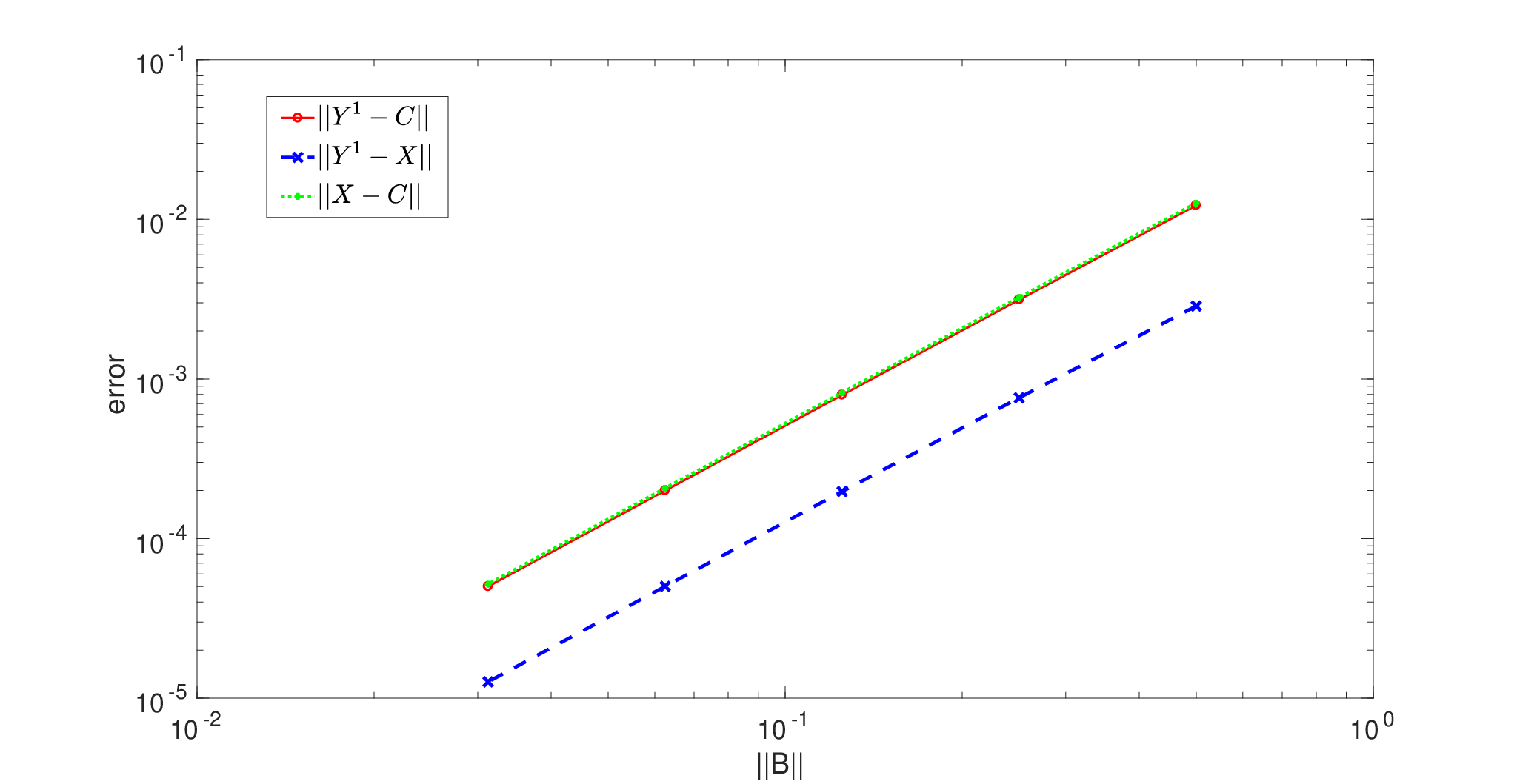
We compare the approximation , computed with one time step of the recursive TTN integrator with step size , with a different retraction, denoted by , obtained by computing the full addition and recursively retracting to the manifold for each . For the latter, we use the built-in function tucker_als of the Tensor Toolbox Package [2]; we recursively apply the function to the full tensor and its retensorized basis matrices.
These comparisons are illustrated in Figure 2 where the norm of is varied. We observe both retractions and have very similar error, and their difference is considerably smaller than their errors. Decreasing the norm of the tensor reduces the approximation error as expected, proportional to . This behaviour of the TTN integrator used for retraction is the same as observed for the Tucker integrator in [21] for the analogous problem of the addition of a Tucker tensor of given multilinear rank and a tangent tensor.
The advantage of the retraction via the TTN integrator is that the result is completely built within the tree tensor network manifold. No further retraction is needed, which is favorable for storage and computational complexity.
7.2 Verification of the exactness property
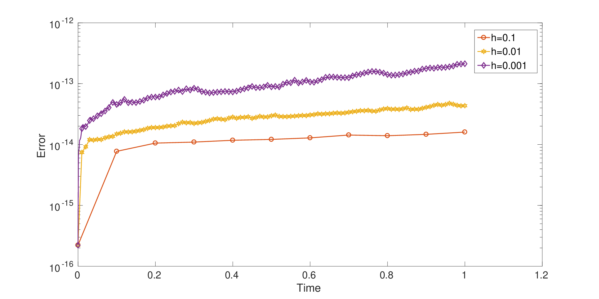
We consider a tree tensor network . For each subtree , let be a skew-symmetric matrix which we choose of Frobenius norm 1. We consider a time-dependent tree tensor network such that with basis matrices propagated in time through
and the connection tensors changed according to
The time-dependent tree tensor network does not change rank and as predicted by Theorem 12, it is reproduced exactly by the recursive TTN integrator, up to round-off errors. The absolute errors calculated at time with step sizes until time are shown in Figure 3.
Acknowledgements
We thank two anonymous referees for their helpful comments on a previous version.
This work was funded by the Deutsche Forschungsgemeinschaft (DFG, German Research Foundation) — Project-ID 258734477 — SFB 1173 and DFG GRK 1838.
References
- [1] P.-A. Absil and I. V. Oseledets. Low-rank retractions: a survey and new results. Comput. Optim. Appl., 62(1):5–29, 2015.
- [2] B. W. Bader, T. G. Kolda, et al. Matlab tensor toolbox version 2.6. Available online, February 2015.
- [3] D. Bauernfeind and M. Aichhorn. Time dependent variational principle for tree tensor networks. arXiv preprint arXiv:1908.03090, 2019.
- [4] L. De Lathauwer, B. De Moor, and J. Vandewalle. A multilinear singular value decomposition. SIAM J. Matrix Anal. Appl., 21:1253–1278, 2000.
- [5] L. Einkemmer and C. Lubich. A low-rank projector-splitting integrator for the Vlasov-Poisson equation. SIAM J. Sci. Comput., 40(5):B1330–B1360, 2018.
- [6] A. Falcó, W. Hackbusch, and A. Nouy. Geometric structures in tensor representations (final release). arXiv preprint arXiv:1505.03027, 2015.
- [7] A. Falcó, W. Hackbusch, and A. Nouy. Tree-based tensor formats. SeMA J., pages 1–15, 2018.
- [8] W. Hackbusch. Multigrid methods and applications, volume 4 of Springer Series in Computational Mathematics. Springer-Verlag, Berlin, 1985.
- [9] W. Hackbusch. Tensor Spaces and Numerical Tensor Calculus. Springer, 2012.
- [10] J. Haegeman, C. Lubich, I. Oseledets, B. Vandereycken, and F. Verstraete. Unifying time evolution and optimization with matrix product states. Physical Review B, 94(16):165116, 2016.
- [11] U. Helmke and J. B. Moore. Optimization and dynamical systems. Communications and Control Engineering Series. Springer-Verlag, London, 1994.
- [12] E. Kieri, C. Lubich, and H. Walach. Discretized dynamical low-rank approximation in the presence of small singular values. SIAM J. Numer. Anal., 54:1020–1038, 2016.
- [13] B. Kloss, Y. B. Lev, and D. R. Reichman. Studying dynamics in two-dimensional quantum lattices using tree tensor network states. arXiv preprint arXiv:2003.08944, 2020.
- [14] O. Koch and C. Lubich. Dynamical low-rank approximation. SIAM J. Matrix Anal. Appl., 29(2):434–454, 2007.
- [15] T. G. Kolda and B. W. Bader. Tensor decompositions and applications. SIAM Review, 51:455–500, 2009.
- [16] P. Kramer and M. Saraceno. Geometry of the time-dependent variational principle in quantum mechanics, volume 140 of Lecture Notes in Physics. Springer-Verlag, Berlin-New York, 1981.
- [17] C. Lubich. From quantum to classical molecular dynamics: reduced models and numerical analysis. Zurich Lectures in Advanced Mathematics. European Mathematical Society (EMS), Zürich, 2008.
- [18] C. Lubich. Time integration in the multiconfiguration time-dependent Hartree method of molecular quantum dynamics. Appl. Math. Res. Express, 2015:311–328, 2015.
- [19] C. Lubich and I. V. Oseledets. A projector-splitting integrator for dynamical low-rank approximation. BIT, 54:171–188, 2014.
- [20] C. Lubich, I. V. Oseledets, and B. Vandereycken. Time integration of tensor trains. SIAM J. Numer. Anal., 53:917–941, 2015.
- [21] C. Lubich, B. Vandereycken, and H. Walach. Time integration of rank-constrained Tucker tensors. SIAM J. Numer. Anal., 56:1273–1290, 2018.
- [22] I. V. Oseledets. Tensor-train decomposition. SIAM J. Sci. Comput., 33(5):2295–2317, 2011.
- [23] D. Perez-García, F. Verstraete, M. M. Wolf, and J. I. Cirac. Matrix product state representations. Quantum Information and Computation, 7(5-6):401–430, 2007.
- [24] Y.-Y. Shi, L.-M. Duan, and G. Vidal. Classical simulation of quantum many-body systems with a tree tensor network. Physical Review A, 74(2):022320, 2006.
- [25] A. Uschmajew and B. Vandereycken. The geometry of algorithms using hierarchical tensors. Linear Algebra Appl., 439(1):133–166, 2013.
- [26] H. Wang and M. Thoss. Multilayer formulation of the multiconfiguration time-dependent Hartree theory. J. Chem. Phys., 119(3):1289–1299, 2003.