Numerical Solution of Inverse Problems by Weak Adversarial Networks
Abstract
In this paper, a weak adversarial network approach is developed to numerically solve a class of inverse problems, including electrical impedance tomography and dynamic electrical impedance tomography problems. The weak formulation of the PDE for the given inverse problem is leveraged, where the solution and the test function are parameterized as deep neural networks. Then, the weak formulation and the boundary conditions induce a minimax problem of a saddle function of the network parameters. As the parameters are alternatively updated, the network gradually approximates the solution of the inverse problem. Theoretical justifications are provided on the convergence of the proposed algorithm. The proposed method is completely mesh-free without any spatial discretization, and is particularly suitable for problems with high dimensionality and low regularity on solutions. Numerical experiments on a variety of test inverse problems demonstrate the promising accuracy and efficiency of this approach.
Keywords— Inverse Problem; Deep learning; Weak formulation; Adversarial network; Stochastic gradient.
1 Introduction
Inverse problems (IP) are ubiquitous in a vast number of scientific disciplines, including geophysics [51], signal processing and imaging [7], computer vision [42], remote sensing and control [58], statistics [36], and machine learning [24]. Let be an open and bounded set in , then an IP defined on can be presented in a general form as:
| (1a) | ||||
| (1b) | ||||
where specifies a differential equation, in which is the solution and the coefficient in the inverse medium problem or the source function in the inverse source problem. Equation can be an ordinary differential equation (ODE), or a partial differential equation (PDE), or an integro-differential equation (IDE), that needs to satisfy (almost) everywhere inside the region . The boundary value (and initial value if applicable) is given by on . Depending on specific applications, partial information of and/or may be available in the interior of . Then IP (1) is to find that satisfies both (1a) and (1b).
To instantiate our approach, we mostly use the classical inverse conductivity problem in electrical impedance tomography (EIT) [11, 38] as an example to present our main idea and the derivations in this paper. However, our methodology can be readily applied to other classes of IPs with modifications. An example of dynamic EIT problem will be shown in Section 4. The goal of EIT is to determine the electrical conductivity distribution of an unknown medium defined on based on the potential , the current measurements, and the knowledge of (and hence ) on/near the boundary of the domain :
| (2a) | ||||
| (2b) | ||||
where is the measured voltage, is the conductivity near the surface of the object and with being the outer normal of . Note that our approach is not to estimate the Dirichlet-to-Neumann (DtN) map associated with the conductivity function as in classical methods specific to the EIT problem [13, 22, 41]. Instead, our goal is to directly solve a general class of IPs (1) numerically using the given data, with the EIT problem (2) as a prototype example without exploiting its special structure (e.g., the DtN map). To make our presentation concise and focused, we only consider IPs with characterized by PDEs in (1a), and assume that the given IP is well-defined and admits at least one (weak) solution.
Our approach is to train deep neural networks that can represent the solution of a given IP, with substantial improvement over classical numerical methods especially for problems with high dimensionality. More specifically, we leverage the weak formulation of the PDE (1a) and convert the IP into an operator norm minimization problem of and . Then we parameterize both , the unknown coefficient , and the test function as deep neural networks , , and respectively, with network parameters , and form a minimax problem of a saddle function of the parameters . Finally, we apply the stochastic gradient descent method to alternately update the network parameters so that gradually approximates the solution of the IP. The parameterization of using deep neural networks requires no discretization of the spatial and temporal domain, and hence is completely mesh free. This is a promising alternative compared to the classical finite difference method (FDM) and finite element methods (FEM) which suffer the issue of the so-called curse of dimensionality, a term first used in [6]. Moreover, our approach combines the training of the weak solution (primal network) and the test function (adversarial network) governed by the weak formulation of the PDE, which requires less regularity of the solution and can be more advantageous in many real-world applications when the solution has singularities.
The remainder of this paper is organized as follows. We first review the recent work on deep learning based solutions to forward and inverse problems in Section 2. In Section 3, we provide the detailed derivation of our method and a series of theoretical results to support the validity of the proposed approach. We discuss several implementation techniques that can improve practical performance and conduct a series of numerical experiments to demonstrate the effectiveness of the proposed approach in Section 4. Section 5 concludes this paper with some general remarks.
2 Related Work
The past few years have witnessed an emerging trend of using deep learning based methods to solve forward and inverse problems. These methods can be roughly classified into two categories. The first category includes methods that approximate the solution of a given problem based on supervised learning approaches. These methods require a large number of input-output pairs through numerical simulation and experiments to train the desired networks. In this category, deep neural networks are used to generate approximate intermediate results from measurement data for further refinement [49, 46, 21, 55, 59, 54], applied to improve the solution of classical numerical methods in the post-processing phase [34, 39, 5, 30, 47, 28, 27, 57], or approximate the mapping from given parameters of an inverse problem to its solution but require spatial discretization and cannot be applied to high-dimensional problems [33, 2, 44].
The second category features unsupervised learning methods that directly solve the forward or inverse problem based on the problem formulation rather than additional training data, which can be more advantageous than those in the first category in practice. For example, feed-forward neural networks are used to parameterize the coefficient functions and trained by minimizing the performance function in [14]. In [40], a neural network architecture called SwitchNet is proposed to solve the inverse scattering problem through the mapping between the scatterers and the scattered field. In [19], a deep learning approach specific to 2D and 3D EIT problems is developed to represent the DtN map by a compact neural network architecture. The backward stochastic differential equation (BSDE) corresponding to the PDE in a forward problem is parameterized in part by neural networks, such that the solution of the PDE can be obtained by integrating the BSDE for a target point in the domain [29, 17, 9]. In [18], the solution of a forward problem is parameterized as a deep neural network, which is trained by minimizing the loss function composed of the energy functional associated with the PDE and a penalty term on the boundary value condition. Another mesh-free framework, called physics-informed neural networks (PINN), for solving both the forward and inverse problems using deep neural networks based on the strong formulation of PDEs is proposed in [52], where a constant coefficient function is considered for the inverse problem part. Specifically, PINN parameterizes the unknowns of a given PDE using deep neural networks, which are trained by minimizing the loss function formed as the least squares of the violation of the PDE at sampled points in the domain and boundary conditions. Some empirical study of PINN is also conducted in [15]. Solutions to IPs based on PINN with data given in problem domain are also considered in [35], and refinement of solutions using adaptively sampled collocation points is proposed in [4]. In [60], the weak formulation of the PDE is leveraged as the objective function, where the solution of the PDE and the test function are both parameterized as deep neural networks trying to minimize and maximize the objective function, respectively. In [37], a similar variational form is used where the test function is fixed basis instead of neural networks to be learned. In [48], three neural networks, one for low-fidelity data and the other two for the linear and nonlinear functions for high-fidelity data, are used by following the PINN approach. The PINN with a multi-fidelity network structure is also proposed for stochastic PDE cases, where polynomial chaotic expansions are used to express the solutions, i.e., as a linear combination of random basis with coefficient functions to be learned [10]. In [8], the solution of an IP is parameterized by deep neural network and learned by minimizing a cost function that enforces the conditions of IP and additional regularization, where solutions to the PDE are required during the training.
Recently, meta-learning based approaches for forward problems are also considered [10, 20, 45]. In [20], the mapping from the coefficient of a differential operator to the pseudo-differential operator (e.g., the Green function) is learned by leveraging the compressed form of the wavelet transform. In [45], a deep operator network consisting of a branch network and a trunk network is introduced. The network encodes the input function evaluated at a finite number of locations (branch-net) and the locations for the output function (trunk-net) and, the output function is given by the inner product of the two plus a bias. Learning network width and depth parameters are also considered using Bayesian optimization in [10].
Our approach to the IP follows our earlier work [60] for forward problems, which differs from the aforementioned existing methods in the use of the weak formulation of PDEs. The weak formulation is a powerful approach for solving PDEs as it requires less regularity and allows for necessary singularities of the solutions, which is an important feature appreciated in many real-world applications such as imaging and abnormality detections. From the theoretical point of view, our method employs neural network parameterizations of both the solution (as the primal network) and the test function (as the adversarial network), and performs an adversarial training in a way that the test function critics on the solution network where the PDE is violated, and the solution network corrects itself at those spots until the PDE is satisfied (almost) everywhere in the domain. However, as inverse problems are often ill-posed and more difficult to solve than forward problems in general, we mostly focus on the inverse problem (2) in EIT in this work. Some experimental results on similar problems are also presented in Section 4.
The adversarial training in the present work has a similar flavor as the one used in generative adversarial network [25], where a generator network is aimed at mapping generic random samples (such as those from a given multivariate Gaussian) to ones following the same distribution as the training samples, and a discriminator network is to distinguish these samples produced by the generator network from the true samples. The generator and adversarial networks act as the two players in a zero-sum game, and are alternately updated by gradient descent and ascent on the objective function respectively to reach an equilibrium. In particular, a notable variant of GAN, called Wasserstein GAN [3], also has a min-max structure of a primal network (generator) and adversarial network (dual function of optimal transport due to the Wasserstein distance between generated and sample distributions) as our formulation. However, WGAN requires its dual function in the max problem to be 1-Lipschitz, which is very difficult to realize numerically and has generated a series of followup work to overcome the issue [26, 50], Spectral Normalization for Generative Adversarial Networks. In contrast, the structure of weak solution versus test function in our work arises naturally from the weak formulation in the PDE theory, which enjoys numerous theoretical justifications and computational benefits for solving IPs for PDEs without imposing restrictive constraint on the adversarial network (test function), as we show in the present work.
In contrast to many existing deep learning methods that require a large amount of demonstration data (e.g., coefficient/boundary value and solution pairs) for training, our method follows an unsupervised learning strategy and only needs the formulation of the PDE and boundary conditions in the given IP. In [56], an unsupervised learning study reveals that generic convolutional neural networks (CNN) automatically bias towards smooth signals and can produce results similar to some sophisticated reconstructions in image denoising without any training data. This phenomenon, known as deep image prior (DIP), is further exploited in [31, 16]. The most notable difference between DIP and the present work is that, our method is completely mesh-free and does not require any spatial discretization, which is suitable for high-dimensional problems. In DIP and its followup works, on the other hand, the reconstruction network is applied to discretized 2D or 3D images. Moreover, our goal is to use the representation power of deep networks to parameterize the solution of an IP in continuous space, whereas the main interests in DIP are on its intriguing automatic regularization properties.
3 Weak Adversarial Network for Inverse Problems
The proposed weak adversarial network approach for IPs is inspired by the weak formulation of PDEs. To obtain the weak formulation of the PDE in (1a), we multiply both sides of (1a) by an arbitrary test function (the Hilbert space of functions with bounded first-order weak derivatives and compactly supported in ) and integrate over :
| (3) |
One of the main advantages of weak formulation (3) is that we can subsequently apply integration by parts to transfer certain gradient operator(s) in to , such that the requirement on the regularity of (and if applicable) can be reduced. For example, in the case of inverse conductivity problem (2), the integration by parts and the fact that on together yield
| (4) |
where is not necessarily differentiable as in (2) in the classical sense anymore (we use to denote the gradient operator with respect to , and as the gradient with respect to and so on in this paper). We call a weak solution (or generalized solution) of the inverse problem (1) if satisfies the boundary condition (1b) and (3) for all . Here is the Lebesgue space of square integrable functions on , and is the Hilbert space of functions with bounded first-order weak derivatives. Note that any classical (strong) solution of (1) is also a weak solution. In this work, we seek for weak solutions of inverse problem (1) so that we may be able to provide an answer to the problem even if it does not admit a solution in the classical sense.
Following the work [60], we consider the weak formulation of the PDE in (1). To cope with the unknown solution and parameter of the PDE in an inverse problem, we parameterize both and as deep neural networks, and consider as a linear functional such that as defined in (3). We define the norm of induced by the norm as
| (5) |
where the -norm of is given by . Therefore, is a weak solution of (1) if and only if and on . As , we know that a weak solution to (1) thus solves the following problem in observation of (5):
| (6) |
among all , and attains minimal value . This result is summarized in the following theorem, and the proof is provided in Appendix A.1.
Theorem 1.
Suppose that satisfies the boundary condition , then is a weak solution of (1) if and only if .
Theorem 1 implies that, to find the weak solution of (1), we can instead seek for the optimal solution that satisfies and meanwhile minimizes (6) by achieving minimum operator norm value due to the nonnegativity of the operator norm. In other words, is a weak solution of the problem (1) if and only if both and vanish. Therefore, we can solve from the following minimization problem which is equivalent to (1):
| (7) |
and is a weight parameter that balances the two terms in the objective function . Note that both terms of the objective function in (7) are nonnegative and vanish simultaneously only at a weak solution of (1).
A promising alternative to classical numerical methods for high-dimensional PDEs is the use of deep neural networks since they do not require domain discretization and are completely mesh free. Deep neural networks are compositions of multiple simple functions (called layers) so that they can approximate rather complicated functions. Consider a simple multi-layer neural network as follows:
| (8) |
where the th layer is given by with weight and bias for , and the network parameters of all layers are collectively denoted by as follows,
| (9) |
Throughout, all vectors in this paper are column vectors by default. In (8), is the input of the network, is the problem dimension of (1) (also known as the size of input layer), and are parameters in the last th layer (also called the output layer). Typical choices of the nonlinear activation function include sigmoid function , hyperbolic tangent (tanh) function , and rectified linear unit (ReLU) function , which are applied componentwisely. The training of deep neural networks refers to the process of optimizing using available data or constraints such that the function can approximate the (unknown) target function. More details about deep neural networks can be found in [24].
Despite of the simple structures like (8), deep neural networks are capable to approximate rather complicated continuous function (and its derivatives if needed) uniformly on a compact support . This significant result is known as the universal approximation theorem [32]. The expressive power of neural networks ensured by the universal approximation theorem suggests a promising mesh-free parameterization of the weak solution of (1). In what follows, we select sufficiently deep neural network structures of form (8) for both and . Specific structures, i.e., layer number and sizes , used in our numerical experiments will be provided in Section 4. Note that and are two separate networks, but we use a single letter to denote their network parameters rather than and to simplify notations. That is, we parameterize as deep neural networks , and attempt to find the parameter such that solves (7). To this end, the test function in the weak formulation (3) is also parameterized as a deep neural network in a similar form of (8) and (9) with parameter denoted by . With the parameterized and , we follow the inner product notation in (3) and define
| (10) |
Instead of normalizing by as in the original definition of (squared) operator norm (5), we approximate (up to a constant scaling of) the squared operator norm in (5) by the following max-type function of :
| (11) |
where is a prescribed bound to constrain the magnitude of network parameter . Here , and stands for the th entry of a matrix , and the th component of a vector . It is worth noting that the bound constraint on the -norm of in (11) is similar to the weight clipping (equivalent to bound on -norm) method used in WGAN [3]. However, they serve different purposes: the constraint in (11) is introduced so that the integrals, such as (4), are bounded (the actual value of this bound can be arbitrary). In this case, the stochastic gradients obtained by the Monte-Carlo approximations in our numerical implementation have bounded variance, which is needed in the proof of Theorem 4 below. On the other hand, the weight clipping in WGAN is to ensure the dual function realized by the neural network is in the class of -Lipschitz functions . As noted in [3], weight clipping is a simple but not appropriate way to implement the -Lipschitz constraint, and hence there is a series of followup work to tackle this issue, such as [26, 50].
Furthermore, we define the loss function associated with the boundary condition (1b) by
| (12) |
For instance, if the boundary condition of is given in (2b) with known boundary value , then . Finally, we define the total loss function , and solve the following minimization problem of its optimal :
| (13) |
where we also constrain on the magnitude of the parameter such that for the same to simplify notation. Note that here both and are finite dimensional vectors, and , hence it is possible to apply numerical optimization algorithms to find the minimizer of .
A standard approach to solving a minimization problem like (13) is the projected gradient descent method which performs the following iteration:
| (14) |
where is the projection of to the ball centered at origin with radius , and is the step size. As we can see, the main computation of (14) is on the gradient . The computation of is straightforward as shown later. The loss , however, is defined as a maximization problem (11), and we need to write its gradient as a function of first. To this end, we have the following lemma to compute the gradient , and the proof is provided in Appendix A.2.
Lemma 2.
Suppose is defined in (11). Then the gradient at any is given by , where is a solution of for the specified .
Remarks.
The exact gradients of and require integrations of functions parameterized by deep neural networks over and in continuous space, which are computationally intractable in practice. Therefore, we use Monte-Carlo (MC) approximations of these integrals. To this end, we need the following result on the approximation of integrals using samples, and the proof is provided in Appendix A.3.
Lemma 3.
Suppose is bounded, and is a probability density defined on such that for all . Given a function , denote . Let be independent samples drawn from . Consider the following estimator of :
| (15) |
Then the first and second moments of are given by
| (16) |
Hence the variance of is . In particular, with the uniform distribution , the variance of is .
Remarks.
We have several remarks regarding Lemma 3:
- •
The estimator of the integral is unbiased.
- •
The variance of shown above decreases at the rate of in the number of sample collocation points. By Hölder’s inequality and that is a probability density, we know
which also verifies that . More importantly, the equalities hold if does not change sign and . Therefore, we can set as close to (up to a normalizing constant) as possible to reduce the variance, but meanwhile ensure is easy to sample from and evaluate as required in (15). This is closely related to the concept of importance sampling.
- •
Lemma 3 provides a feasible way to approximate the gradient of for (14). For instance, to compute , we can take gradient of (12) with respect to , sample collocation points on the boundary and approximate by summation of function evaluations at the sample points. If we take and uniformly sample , the estimate becomes
| (17) | ||||
Similarly, we can compute the stochastic gradient of . In the case of taking in with given, and uniformly sampling collocation points inside the region , can be estimated by
| (18) | ||||
where and its estimator are given by
and is a solution of the maximization problem (11) according to Lemma 2. All integrals in the gradients can be approximated in a similar way. These approximated gradients are in fact stochastic gradients, which are unbiased and have bounded variances due to the boundedness of the network parameters. With these approximations, (14) reduces to the stochastic projected gradient descent method, which ensures convergence to a local stationary point of (13) with proper choice of step sizes. Since (13) is constrained, the gradient mapping, defined by , is used as the convergence criterion of [23, 43, reddi2016proximal]. Note that the definition of gradient mapping takes the normalization of step size into consideration. Moreover, without the projection , the gradient mapping reduces to , whose magnitude is an evaluation criterion for local stationary points (i.e., ) for unconstrained case. This result is stated in the following theorem, and the proof is given in Appendix A.4.
Theorem 4.
Remarks.
Theorem 4 establishes the convergence and iteration complexity of (14) to the so-called -solution of the problem. The result is based on the expected magnitude of the gradient mapping, which is a standard convergence criterion in nonconvex constrained stochastic optimization. However, this only ensures approximation to a stationary point (not necessarily a local or global minimizer) on expectation. In theory, one can apply additional global optimization techniques to (7) in order to find a global minimizer (possibly only with high probability at best) with substantially higher computational cost. However, we will not exploit this issue further in this work.
Now we summarize the steps of our algorithm for solving IPs using weak adversarial networks. To simplify the presentation, we introduce the following notation to indicate the stochastic gradient descent (SGD) procedure for finding a minimizer of a loss function :
| (19) |
which means the output is the result after we execute the (projected) SGD scheme with step size below for with initial :
| (20) |
Here is the set of sampled collocation points, is the gradient of the loss function to be minimized, and stands for the stochastic approximation of at any given , where the integrals are estimated as in (15) using the sampled collocation points . Therefore, each iteration of our algorithm consists of two steps. In Step 1, we fix and solve the maximization problem with objective function defined in (11) by applying stochastic gradient ascent for steps to obtain an approximate maximizer ; In Step 2, we fix this , and update by one stochastic gradient descent step using gradient . Then we go to Step 1 to start the next iteration. Hence, our objective function is , for which we seek for the optimal point via a min-max optimization . This procedure is referred to Inverse Problem Solver using Weak Adversarial Network (IWAN) and summarized in Algorithm 1. The parameter values in our numerical implementations are presented in Section 4.
4 Numerical Experiments
4.1 Implementation Details
In this subsection, we discuss several implementation details and modifications regarding Algorithm 1. First, to avoid spending excessive time in solving the inner maximization problem in (11) with a fixed , we only apply a few iterations to compute . Then we switch to update for one iteration. See the two SGD steps in Algorithm 1. This can improve overall efficiency and avoid spending excessive time on the inner maximization problem of , especially when is still far from optimal yet. In fact, we can employ two separate test functions and (we again use the same for notation simplicity). In each iteration , we alternately update in order, each with one or a few SGD steps (20). We will specify the numbers of steps for these networks for our experiments below.
During the derivations in Section 3, we require bounded network parameters and , where the bound can be arbitrarily large, to ensure finite variances of the integral estimators using samples so that the SGD is guaranteed to converge. An alternative way to handle the boundedness constraints is to add and as regularization terms to the objective function in (7). One can also use the operator norm (5) with denominator replaced by (approximated by MC similarly as in (15)), which is also adopted in our implementation. This replacement does not cause issue in numerical implementation since the test function is realized by a network with fixed width/depth and bounded parameters, and hence is guaranteed to be in .
A test function is required to vanish on in the weak formulation (3). One simple technique to ensure this is to precompute a function such that if and if (e.g., a distance function to would work). Then we seek for a parameterized network with no constraint on its arbitrary boundary, and set the test function to which still takes zero value on .
We implemented our algorithm using TensorFlow [1] (Python version 3.7), a state-of-the-art deep learning package that can efficiently employ GPUs for parallel computing. The gradients with respect to network parameters ( and ) and input () are computed by the TensorFlow builtin auto-differentiation module. During training, we can also substitute the standard SGD optimizer by many of its variants, such as AdaGrad, RMSProp, Adam, Nadam etc. In our experiments, we use AdaGrad supplied by the TensorFlow package, which appears to provide better performance than other optimizers in most of our tests. All other parameters, such as the network structures (numbers of layers and neurons), step sizes (also known as the learning rates), number of iterations, will be specified in Section 4.
4.2 Experiment Setup
In this section, we conduct a set of numerical experiments to show the practical performance of Algorithm 1 in solving inverse problems. To quantitatively evaluate the accuracy of an approximate solution , we use the relative error (in the sense) of to the ground truth , defined by , where . In practice, we compute by evaluating on a fixed set of mesh grid points in . More specifically, we used a regular mesh grid of size for , and sampled one point for each of these grid points, i.e., for each grid point , randomly draw values of the other coordinates within the domain such that . These points were sampled in advance and then used for all comparison algorithms to compute their test relative error. Note that these points are different from those sampled for training in these methods.
In all of our experiments, we parameterize each of as a 9-layer fully connected neural network with 20 neurons per layer as in (8) unless otherwise noted. We set to tanh for , softplus for , sinc for in , and tanh for , elu for , and sigmoid for in . We use elu in the output layer of . In parallel, we set to tanh for and sinc for in and . Unless otherwise noted, we apply one SGD update with step size to both of and (each of them performs the update in Algorithm 1), and two () SGD updates with step size to both of and (each of them performs the update in Algorithm 1), following the order of in every iteration of Algorithm 1. We set the weight for the boundary loss function in (7), but also set a weight to and specify its value in the experiment. Other parameters will also be specified below. All the experiments are implemented, trained, and tested in the TensorFlow framework [1] on a machine equipped with Intel 2.3GHz CPU and an Nvidia Tesla P100 GPU and 16GB of graphics card memory.
4.3 Experimental Results on Inverse Conductivity Problems
Test 1: Inverse conductivity problem with smooth . We first test our method on the inverse conductivity problem (2) with a smooth conductivity distribution . In this test, we set with problem dimension . The setup for the ground truth conductivity distribution , the ground truth potential and the source term are provided in the table 1 which is in the appendix B. We set and , , and run Algorithm 1 for iterations. The true and the point-wise error (with relative error ) are shown in Figure 1(a) and 1(b) respectively. The progress of the relative error of versus iteration number is shown in Figure 1(c) (all plots of relative error versus iteration number in this section are shown using moving average with a window size ). For the demonstration purpose, only the cross sections that have main spatial variations are shown (same for the other test results below).
Test 2: Inverse conductivity problem with nearly piecewise constant . We consider (2) with a less smooth, nearly piecewise constant conductivity . In this test, we set , define where and , and set to in and in . For ease of implementation, we slightly smooth the ground truth conductivity. One can find the setup of the smoothed conductivity , the ground truth potential , and the source term in the table 1. Then we solve the inverse problem (2) with dimensionality . We set and , and for respectively. In each case, we run Algorithm 1 for iterations, and obtain relative errors for , respectively. The recovery results are shown in Figure 2. Figure 2(a) shows the ground truth (left) and the progress of relative errors versus iteration number for different (right). The pointwise absolute errors for these dimensions are shown in Figure 2(a).
Test 3: Inverse conductivity problem with noisy measurements. Under the same experiment setting as Test 2, we solve the inverse problem (2) where the measurement data are perturbed by random noise for the case. Specifically, we scale every measurement data value by , , where is drawn independently from the standard normal distribution every time, followed by a truncation into interval . We do not perturb . The results are given in Figure 3 in parallel to the noiseless case above, where Figure 3(a) shows the ground truth conductivity (left) and the progress of relative error of versus iteration number (right). The pointwise absolute error after 20,000 iterations with noise levels are shown in Figure 3(b). We observe that the progress becomes more oscillatory due to the random measurement noise in Figure 3(a), and the final reconstruction error is larger for higher noise level in Figure 3(b) as expected.
Test 4: Inverse conductivity problem with different features in . We consider several cases with more challenging ground truth conductivity . The first case has with two disjoint modes. We define , and set and , where , , , and . We set the conductivity to in , in , and in . We also smooth using a Gaussian kernel. The setup of the ground truth conductivity , the ground truth potential , and the source function are provided in the table 1 (see Test 4(1)). We set , , , and run Algorithm 1 for iterations. Figure 4(a) shows the ground truth (left) and the recovered conductivity with relative error (right). Figure 4(c) plots the progress of relative error of versus iteration number. In the second case, we follow the same setting but define (which has sharp corner) and where , , and set in and in . We again smooth and provide the ground truth conductivity , the ground truth potential , and the source function in the table 1 (see Test 4(2)). We set and again run Algorithm 1 for iterations. The recovered (with relative error ) and the progress of relative error are shown in Figure 4(d) and 4(f) respectively. Lastly, we consider a non-convex shaped , and show the recovered (with relative error ) and the progress of relative error in Figure 4(g) and 4(i) respectively. We set the domain and define , where and . We set in and in and in . Once again, we sightly smooth the conductivity and provide the setup of the ground truth conductivity , the ground truth potential and the source function in the table 1 (see Test 4(3)).
Test 5: EIT problem. We consider an artificial 5D EIT problem (2) on but replace (2b) with a different boundary condition given by on , where is the outer normal vector at the boundary point. We define and . We set ground truth conductivity and potential , and compute the corresponding boundary value as our input data. We set the source term in (2a), , , , and run Algorithm 1 for 20,000 iterations. The cross section of the recovered (with relative error ) and the progress of relative error versus iteration number are shown in Figure 5(a) and 5(b), respectively.
Test 6: Inverse thermal conductivity problem involving time. We consider an inverse thermal conductivity problem of (1) with temporally varying as follows,
| (21a) | ||||
| (21b) | ||||
| (21c) | ||||
where and the final time , is the thermal conductivity, indicates the temperature and is the source function which indicates the rate of heat generation per unit volume, where is the unit outer normal vector of , for is the given initial value, and for are given boundary values. In this problem, we would like to recover the thermal conductivity which is a function of the temperature in the standard setting, but we simply treat as a function of in our experiment here. We set the source function as follows,
where , the initial value , the Neumann boundary value of as . We set the ground truth where , , and , and use noisy boundary value measurements and , where is independently drawn for and and all from the standard normal distribution followed by a truncation to , and the noise levels are set to . We consider the case with problem dimension , and set , , and . The results are shown in Figure 6, where Figure 6(a) plots the sampled values of recovered in comparison with the ground truth relation , and Figure 6(b) shows the progress of relative error of versus iteration number for the three different noise levels. The reconstructions of are all faithful, while higher noise levels decreases the accuracy and make convergence to true solution more challenging.
Test 7: Comparison with PINN. We compare the proposed method with a state-of-the-art method called physics-informed neural networks (PINNs) [52]. PINN is also a deep-learning based method designed for solving forward problem as well as inverse problem for PDEs. PINN is based on the strong form of the PDEs, where the loss function in the minimization problem of PINN consists of the sum of squared errors in the violation of the PDE and the boundary condition at points sampled inside and on , respectively. In contrast, our method is based on the weak form of PDE which employs a test function and yields a min-max problem to better tackle singularities of the problem. We first compare the proposed method and the PINN method in the problem in Test 1. Note that PINN was only applied to inverse conductivity problem with constant conductivity in [52], it is straightforward to extend this method to non-constant conductivity by also parameterizing the conductivity as an additional deep neural network. In this problem, we take with . For the PINN method, we also parameterize as a 9-layer fully-connected network with neurons in each hidden layer and tanh as activation functions in all hidden layers. For , we parameterized it by using the same network structure as that used for the proposed method in Test 1. We let the weight of the boundary term in the loss function is and use the builtin Adam optimizer of TensorFlow with learning rate to update the network parameters in PINN. For fair comparison, we also use the Adam optimizer with learning rate for updating and in the proposed method. The results after 20,000 iterations of both methods are given in Figure 7. In Figure 7(a), we can see the error of obtained by IWAN is much lower than that by PINN. This can also be seen from Figure 7(b), where the error decays very fast for the proposed IWAN. We tried a variety of network structures and parameter settings of PINN and obtain similar results.
We also compared the proposed method and PINN on the inverse conductivity problem in Test 2, where the ground truth conductivity is less smooth and nearly piecewise constant. We use the same parameter settings for both methods as above except for the network structure of , which follows the one in Test 2. The conductivity recovered by PINN and IWAN and the progresses of their relative error versus computation time (in seconds) are given in Figures 7(c) and 7(d), respectively. From Figure 7(d), it appears that PINN cannot get close to the ground truth within 20,000 iterations. Therefore, we rerun PINN for 100,000 iterations, and plot the relative error versus computation time in Figure 7(f), from which it seems that PINN still cannot converge to the desired solution. However, the result obtained by PINN does satisfy the PDE closely, as shown in Figure 7(e): the difference between the two sides of PDE (left), i.e., , is much smaller than (right), but PINN cannot capture the irregularities and singularities of the solution since it is based on the strong form of the PDE. In contrast, IWAN can overcome this issue and recover the weak solution properly. We also show the objective function value of PINN and IWAN in Figures 7(g) and 7(h), respectively (Note that the objective function in IWAN is defined as for min-max optimization, and the objective function of PINN is for minimization only and hence different from IWAN).
by PINN
by IWAN
Test 8: Efficiency improvement using important sampling. As shown in Lemma 3, adaptive sampling may reduce the variance of the sample-based approximation of integrals, which in turn can improve the convergence of stochastic gradient descent. To demonstrate this, we consider the inverse conductivity problem on with problem dimension , ground truth conductivity distribution , where , . We set , on and . For the parameter setup, we use the same setup as that in Test 7. Then we solve this inverse problem using the proposed method IWAN with points in the domain sampled from the uniform distribution as above and also a multivariate normal distribution respectively. Specifically, to obtain multivariate normal samples, we first sample points of from the multivariate normal distribution with mean value and inverse covariance matrix (points outside of is discarded), and then draw each of the remaining coordinates randomly from interval independently. The result was shown in the figure 8. The progress of relative error versus computation time (in second) for iterations is shown in Figure 8, which shows that the convergence using adaptive multivariate normal distribution is faster than that with uniform distribution.
4.4 Empirical Robustness Analysis
We conduct a series of experiments to evaluate the robustness of Algorithm 1 in terms of network structure (number of layers and neurons) and the number of sampled collocation points.
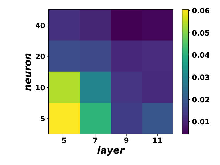
Test 9: Network structure. In this experiment, we test the performance of Algorithm 1 with different network structures, i.e., the layer number (network depth) and the per-layer neuron number (network width) . We test different combinations of and (in each combination we set for all ). More specifically, we apply Algorithm 1 to the inverse conductivity problem (2) in Test 2 above with problem dimension and a total of 16 combinations with and . For each combination , we run Algorithm 1 for iterations and plot the relative error of in Figure 9(a) and the corresponding running time (in seconds) in Figure 9(b). The exact values of errors and running times are present in Table 2 in Appendix C. Based on Figure 9(a), it seems that deeper (larger ) and/or wider (larger ) neural networks yield lower reconstruction error (but at the expense of higher per-iteration computational cost). For fixed layer number , we show the progress of relative error versus iteration number with varying per-layer neuron number in Figure 10(a). Similarly, for fixed per-layer neuron number , we also show the progress of relative error versus iteration number with varying layer number in Figure 10(b). These figures also suggest that larger and yield better accuracy, although the per-iteration computational cost also increases and it may take more iterations to converge.

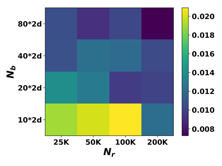

Test 10: Number of sampled collocation points. In Section 3, we showed that the number of sampled collocation points affects the variance of the integral estimator, so that the variance reduces at the order of . In this experiment, we test the empirical effect of the collocation point numbers in the region and on the boundary in Algorithm 1 for the same inverse conductivity problem (2) of dimension in Test 2 above. We choose different combinations of for (K=1,000) and , and keep all other parameters in Test 2 unchanged. We run Algorithm 1 for 20,000 iterations, and plot the final relative error of in Figure 9(c) and the corresponding running time (in seconds) in Figure 9(d). The exact values of errors and running times are present in Table 3 in Appendix C. We also plot the progress of relative error of versus iteration number for fixed K and varying in Figure 11(a), and that for fixed and varying in Figure 11(b). The results in Figure 9(c) and Figure 11 show that larger amounts of collocation points can generally improve accuracy of the reconstruction.
Test 11: Relation between relative error, gradient value and sample points. We conduct an experiment to show the relation between the relative error, the expected value of gradient mapping, and the numbers of collocation points and . In this experiment, we use the Adam optimizer for with learning rate and use the Adagrad optimizer for with learning rate and . We keep other settings unchanged as that used for case K and in Test 10. Then, we solve problem (2) of dimension using the proposed algorithm with K and , where takes value in . After iterations, we evaluate (expectation is approximated by empirical average of 5 runs), the relative error, and the running time for each value of , and plot their values versus in Figures 12(b), 12(c), 12(d), respectively. From Figure 12(b), we can see that is approximately proportional to . Figures 12(c) and 12(d) show that the solution error generally decreases in at the expense of longer computational time. For reference, the relative error versus iteration and running time with varying are shown in Figure 12(a).
5 Concluding Remarks
We have presented a weak adversarial network approach to solve a class of inverse problems numerically. We leverage the weak formulation of PDEs in the inverse problems, and parameterize the unknown solution as primal neural network and the test function as adversarial network. The weak formulation and the boundary conditions yield a saddle function in the parameters of the primal network and adversarial network, which only rely on the inverse problem itself but not any other training data. These parameters are alternately updated until convergence. We provide a series of theoretical justifications on the convergence of our proposed algorithm. Our method does not require any spatial discretization, and can be applied to a large class of inverse problems, especially those with high dimensionality and less regularity on solutions. Numerical experiments have been conducted by applying the proposed method to a variety of challenging inverse problems. The results suggest promising accuracy and efficiency of our approach.
Acknowledgements
GB and YZ are supported in part by NSFC Innovative Group Fund (No.11621101). XY is supported in part by NSF under grants DMS-1620342, CMMI-1745382, DMS-1818886 and DMS-1925263. HZ is supported in part by NSF under grants DMS-1620345 and DMS-1830225, and ONR N00014-18-1-2852.
Appendix A Appendix: Proofs
A.1 Proof of Theorem 1
For ease of presentation, our proof of Theorem 1 here is based on the problem formulation (2). However, it can be easily modified for the PDEs in many other inverse problems.
Proof.
For any fixed and , the maximum of is achievable over since is continuous and is closed in . Define , then due to the definition of operator norm in (5). On the other hand, let , then it is clear that the minimum value of over can be attained at any of the weak solutions. Hence the minimax problem (6) is well-defined.
Now we show that satisfying is the solution of the minimax problem (6) if and only if it is a weak solution of the problem (1). Suppose is a weak solution of the problem (1), namely satisfies (3) for all , then for all . Therefore, , and is the solution of the minimax problem (6). On the other hand, suppose a weak solution of (1) exists. Assume that is a minimizer of the problem (6), i.e., , but not a weak solution of the problem (1), then there exists such that . Therefore . However, as we showed above, since is a weak solution of (1), which contradicts to the assumption that is the minimizer of (6). Hence must also be a weak solution of (1), i.e., satisfies (3). ∎
A.2 Proof of Lemma 2
Proof.
Due to the definition of in (11) and the optimality of , we know that . Therefore, we have
| (22) |
Now we form the Lagrange function for the maximization problem . Then the Karush-Kuhn-Tucker (KKT) condition of is given by
| (23a) | ||||
| (23b) | ||||
| (23c) | ||||
The complementary slackness condition (23b) implies that
| (24) |
If , then we know due to (23a) and hence (22) reduces to . If , then due to (23b), and hence (24) implies . Thus multiplying (23a) by yields , from which we can see (22) also reduces to . ∎
A.3 Proof of Lemma 3
Proof.
The first moment, i.e., expectation of , can be computed as follows:
| (25) |
To compute the second moment of , we first observe that the variance of is
Note that the variance of is
Hence the second moment of is
which completes the proof. ∎
A.4 Proof of Theorem 4
Proof.
Due to the parameterization of using finite-depth neural network (8) and the compactness of , we know and have Lipschitz continuous gradient with respect to for all . As is bounded and , there exists such that has -Lipschitz continuous gradient , since is composed of integrals of and over .
Recall that the projected stochastic gradient descent step (14), started from initial , generates the sequence as follows:
| (26) |
where denotes the stochastic gradient of at using ( resp.) sample collocation points in (on resp.) with . We let denote the true (but unknown) gradient of at , and define a companion sequence using as
| (27) |
Note that is not computed in practice (computation of is not possible as is unknown), but only defined for convergence analysis here. Also note that and are bounded, and hence all integrals of and are bounded, we know is an unbiased estimate of with bounded variance, denoted by , according to Lemma 3. Moreover, Lemma 3 implies that there exists dependent on , , , and only ( is the bound of and due to the boundedness of and ) the integral such that as .
Now we are ready to verify the convergence of the projected SGD iterations (26). First, the -Lipschitz continuity of implies that
| (28) |
where we denote for all . Also due to the -Lipschitz continuity of , we have
| (29) |
where we denote . Note that , whose magnitude is what we want to bound eventually. Furthermore, due to the optimality of in (26) (which is convex in ), we know that
| (30) |
Adding (28), (29), and (30) yields
| (31) |
Repeating (28), (29), (30), and (31) with and replaced by and respectively, and using the optimality of in (27) with , we obtain
| (32) |
| (33) |
Now due to Cauchy-Schwarz inequality, the definitions of and in (26) and (27), and that the projection onto the convex set is a non-expansive operator (i.e., for any ), we can show that
| (34) |
Moreover, we have that
| (35) |
Substituting (34) and (35) into (33), we obtain
| (36) |
Taking expectation on both sides of (36) and discarding the last negative term, we obtain
| (37) |
where we used the fact and the notation . Now taking sum of (37) for , dividing both sides by , and setting (hence and ), we know that
| (38) |
by choosing per-iteration sample complexity and iteration number as where (and hence ). This completes the proof. ∎
Appendix B Appendix: Problem Setting
The functions and parameters used in our experiments are summarized in table 1.
| Problem |
|
|||||||||||||
|---|---|---|---|---|---|---|---|---|---|---|---|---|---|---|
| Test 1 |
|
| ||||||||||||
|
|
|||||||||||||
| Test 4(1) |
|
| ||||||||||||
| Test 4(2) |
|
| ||||||||||||
| Test 4(3) |
|
|
Appendix C Appendix: Recorded errors and running times in Tests 9 and 10
The recorded errors and running times for Test 9 and Test 10 were present in table 2 and table 3, respectively.
| 5 | 0.060347 | 0.040950 | 0.014905 | 0.019489 |
|---|---|---|---|---|
| 10 | 0.053842 | 0.029382 | 0.013325 | 0.011165 |
| 20 | 0.017955 | 0.016862 | 0.010916 | 0.011490 |
| 40 | 0.012390 | 0.010213 | 0.004422 | 0.005309 |
| 5 | 1391.76(s) | 1432.90(s) | 1438.87(s) | 1458.12(s) |
| 10 | 1435.78(s) | 1468.95(s) | 1520.67(s) | 1568.49(s) |
| 20 | 1447.66(s) | 1522.84(s) | 1596.83(s) | 1614.04(s) |
| 40 | 1539.93(s) | 1623.20(s) | 1717.53(s) | 1809.30(s) |
| K | K | K | K | |
|---|---|---|---|---|
| 0.019023 | 0.020007 | 0.020898 | 0.012208 | |
| 0.013999 | 0.012920 | 0.009681 | 0.010050 | |
| 0.010668 | 0.012292 | 0.012053 | 0.010385 | |
| 0.01061 | 0.009207 | 0.010200 | 0.007267 | |
| 528.88(s) | 554.64(s) | 556.08(s) | 552.86(s) | |
| 915.66(s) | 898.32(s) | 932.98(s) | 928.78(s) | |
| 1597.66(s) | 1577.03(s) | 1556.92(s) | 1590.87(s) | |
| 2798.17(s) | 2802.79(s) | 2795.28(s) | 2801.45(s) |
Appendix D Appendix: Comparison with classical numerical methods
To further evaluate the proposed method, we provide an example that compares IWAN and a classical finite difference method (FDM) on a 2D problem in Test 2. We would like to acknowledge an anonymous reviewer for suggesting this valuable comparison. It is worth pointing out that the majority of existing numerical methods, such as FDM, require the knowledge of Dirichlet-to-Neumann (DtN) map for the EIT problem. However, to be consistent with the settings used in the present work, we conduct the comparison with FDM under the same setting of Test 2, where a DtN map is not available but only the boundary conditions of and in (2) are given.
In FDM, we discretize the domain into mesh grids (about unknowns for each of and ). We also experiment with higher resolution but it does not improve solution quality; see later for more explanations. We approximate the partial derivatives in the PDE by finite differences. As the problem is underdetermined, we use regularization and formulate as a minimization problem of , where the objective function is the sum of two terms: the mean square error of the PDE, and the TV regularization on . For comparison, we choose hidden layers with neurons per-layer to parameterize and (each with unknowns). We set the number of collocation points to and (similar to the discretization resolution of FDM). For FDM, we test different regularization hyperparameter (the weight of the TV term), and show the result in Figure 13(a). We observe that FDM achieved the best result when , which is used to generate the other images in Figure 13. The relative error obtained by IWAN is shown in Figure 13(b). Figure 13(c) shows the absolute error obtained by IWAN and FDM ( is the recovered conductivity by IWAN or FDM, and is the ground truth), respectively, which demonstrates that IWAN can faithfully recover but FDM cannot in the setting of Test 2. Figure 13(e) shows the objective function value versus iteration by FDM, which suggests that FDM has converged. We also show obtained by FDM in Figure 13(d), which shows that the obtained by FDM indeed satisfies the PDE approximately. In addition, we increase the domain discretization resolution up to for FDM, but did not observe any noticeable improvement, and hence we omitted the results here.
References
- [1] M. Abadi, P. Barham, J. Chen, Z. Chen, A. Davis, J. Dean, M. Devin, S. Ghemawat, G. Irving, M. Isard, et al. Tensorflow: A system for large-scale machine learning. In 12th USENIX Symposium on Operating Systems Design and Implementation (OSDI 16), 265–283, 2016.
- [2] J. Adler, O. Öktem. Solving ill-posed inverse problems using iterative deep neural networks. Inverse Probl., 33(12):124007, 2017.
- [3] M. Arjovsky, S. Chintala, and L. Bottou. Wasserstein generative adversarial networks. In International Conference on Machine Learning, pages 214–223, 2017.
- [4] C. Anitescu, E. Atroshchenko, N. Alajlan, and T. Rabczuk. Artificial neural network methods for the solution of second order boundary value problems. Computers, Materials & Continua, 59(1):345–359, 2019.
- [5] S. Antholzer, M. Haltmeier, and J. Schwab. Deep learning for photoacoustic tomography from sparse data. Inverse Probl. Sci. Eng., 27(7):987–1005, 2019.
- [6] R. Bellman. Dynamic programming. Science, 153(3731):34–37, 1966.
- [7] M. Bertero and P. Boccacci. Introduction to inverse problems in imaging. CRC press, 1998.
- [8] L. Bar and N. Sochen. Unsupervised deep learning algorithm for pde-based forward and inverse problems. arXiv preprint arXiv:1904.05417, 2019.
- [9] C. Beck, W. E, and A. Jentzen. Machine learning approximation algorithms for high-dimensional fully nonlinear partial differential equations and second-order backward stochastic differential equations. J. Nonlinear Sci., 29(4):1563–1619, 2019.
- [10] X. Chen, J. Duan, and G. E. Karniadakis. Learning and meta-learning of stochastic advection-diffusion-reaction systems from sparse measurements. arXiv preprint arXiv:1910.09098, 2019.
- [11] M. Cheney, D. Isaacson, and J. C. Newell. Electrical impedance tomography. IEEE Signal Process Mag, 41(1):85–101, 1999.
- [12] C. B. Croke, G. Uhlmann, I. Lasiecka, and M. Vogelius. Geometric Methods in Inverse Problems and PDE Control, volume 137. Springer Science & Business Media, 2004.
- [13] E. B. Curtis and J. A. Morrow. The Dirichlet to Neumann map for a resistor network. SIAM J. Appl. Math., 51(4):1011–1029, 1991.
- [14] P. Dadvand, R. Lopez, and E. Onate. Artificial neural networks for the solution of inverse problems. In Proceedings of the International Conference on Design Optimisation Methods and Applications ERCOFTAC, volume 2006, 2006.
- [15] T. Dockhorn. A discussion on solving partial differential equations using neural networks. arXiv preprint arXiv:1904.07200, 2019.
- [16] S. Dittmer, T. Kluth, P. Maass, and D. O. Baguer. Regularization by architecture: A deep prior approach for inverse problems. Journal of Mathematical Imaging and Vision, pages 1–15, 2019.
- [17] W. E, J. Han, and A. Jentzen. Deep learning-based numerical methods for high-dimensional parabolic partial differential equations and backward stochastic differential equations. Communications in Mathematics and Statistics, 5(4):349–380, 2017.
- [18] W. E and B. Yu. The deep ritz method: a deep learning-based numerical algorithm for solving variational problems. Communications in Mathematics and Statistics, 6(1):1–12, 2018.
- [19] Y. Fan and L. Ying. Solving electrical impedance tomography with deep learning. arXiv preprint arXiv:1906.03944, 2019.
- [20] J. Feliu-Faba, Y. Fan, and L. Ying. Meta-learning pseudo-differential operators with deep neural networks. arXiv preprint arXiv:1906.06782, 2019.
- [21] X. Fernández-Fuentes, D. Mera, A. Gómez, and I. Vidal-Franco. Towards a fast and accurate eit inverse problem solver: A machine learning approach. Electronics, 7(12):422, 2018.
- [22] E. Francini. Recovering a complex coefficient in a planar domain from the dirichlet-to-neumann map. Inverse Probl., 16(1):107, 2000.
- [23] S. Ghadimi, G. Lan, and H. Zhang. Mini-batch stochastic approximation methods for nonconvex stochastic composite optimization. Math. Program., 155(1-2):267–305, 2016.
- [24] I. Goodfellow, Y. Bengio, and A. Courville. Deep Learning. MIT press, 2016.
- [25] I. Goodfellow, J. Pouget-Abadie, M. Mirza, B. Xu, D. Warde-Farley, S. Ozair, A. Courville, and Y. Bengio. Generative adversarial nets. In Adv. Neural Inf. Proces. Syst., 2672–2680, 2014.
- [26] I. Gulrajani, F. Ahmed, M. Arjovsky, V. Dumoulin, and A. C. Courville. Improved training of wasserstein gans. In Advances in neural information processing systems, pages 5767–5777, 2017.
- [27] S. J. Hamilton, A. Hänninen, A. Hauptmann, and V. Kolehmainen. Beltrami-net: domain independent deep d-bar learning for absolute imaging with electrical impedance tomography (a-eit). Physiol. Meas., 2019.
- [28] S. J. Hamilton and A. Hauptmann. Deep d-bar: Real-time electrical impedance tomography imaging with deep neural networks. IEEE Trans. Med. Imaging, 37(10):2367–2377, 2018.
- [29] J. Han, A. Jentzen, and E. Weinan. Solving high-dimensional partial differential equations using deep learning. Proceedings of the National Academy of Sciences, 115(34):8505–8510, 2018.
- [30] A. Hauptmann, F. Lucka, M. Betcke, N. Huynh, B. Cox, P. Beard, S. Ourselin, and S. Arridge. Model based learning for accelerated, limited-view 3d photoacoustic tomography. IEEE Trans. Med. Imaging, PP(99):1–1, 2017.
- [31] R. Heckel and M. Soltanolkotabi. Denoising and regularization via exploiting the structural bias of convolutional generators. arXiv preprint arXiv:1910.14634, 2019.
- [32] K. Hornik. Approximation capabilities of multilayer feedforward networks. Neural Netw., 4(2):251–257, 1991.
- [33] A. Joshi, V. Shah, S. Ghosal, B. Pokuri, S. Sarkar, B. Ganapathysubramanian, and C. Hegde. Generative models for solving nonlinear partial differential equations. In Workshop on Machine Learning and the Physical Sciences, 2019.
- [34] K. H. Jin, M. T. Mccann, E. Froustey, and M. Unser. Deep convolutional neural network for inverse problems in imaging. IEEE Trans. Image Process., 26(9):4509–4522, 2017.
- [35] H. Jo, H. Son, H. J. Hwang, and E. Kim. Deep neural network approach to forward-inverse problems. arXiv preprint arXiv:1907.12925, 2019.
- [36] J. Kaipio and E. Somersalo. Statistical and Computational Inverse Problems, volume 160. Springer Science & Business Media, 2006.
- [37] R. Khodayi-Mehr and M. M. Zavlanos. Varnet: Variational neural networks for the solution of partial differential equations. arXiv preprint arXiv:1912.07443, 2019.
- [38] T. A. Khan and S. H. Ling. Review on electrical impedance tomography: Artificial intelligence methods and its applications. Algorithms, 12(5):88, 2019.
- [39] E. Kang, J. Min, and J. C. Ye. A deep convolutional neural network using directional wavelets for low-dose x-ray ct reconstruction. Med. Phys., 44(10):e360, 2017.
- [40] Y. Khoo and L. Ying. Switchnet: a neural network model for forward and inverse scattering problems. arXiv preprint arXiv:1810.09675, 2018.
- [41] M. V. Klibanov, J. Li, and W. Zhang. Convexification of electrical impedance tomography with restricted dirichlet-to-neumann map data. Inverse Probl., 2019.
- [42] N. Paragios, Y. Chen, and O. D. Faugeras. Handbook of mathematical models in computer vision. Springer Science & Business Media, 2006.
- [43] Z. Li and J. Li. A simple proximal stochastic gradient method for nonsmooth nonconvex optimization. In Adv. Neural Inf. Proces. Syst., 5564–5574, 2018.
- [44] H. Li, J. Schwab, S. Antholzer, and M. Haltmeier. NETT: Solving inverse problems with deep neural networks. Inverse Probl., 2020.
- [45] L. Lu, P. Jin, and G. E. Karniadakis. Deeponet: Learning nonlinear operators for identifying differential equations based on the universal approximation theorem of operators. arXiv preprint arXiv:1910.03193, 2019.
- [46] S. Martin and C. T. Choi. Nonlinear electrical impedance tomography reconstruction using artificial neural networks and particle swarm optimization. IEEE Trans. Magn., 52(3):1–4, 2015.
- [47] S. Martin and C. T. Choi. A post-processing method for three-dimensional electrical impedance tomography. Sci Rep, 7(1):7212, 2017.
- [48] X. Meng and G. E. Karniadakis. A composite neural network that learns from multi-fidelity data: Application to function approximation and inverse pde problems. arXiv preprint arXiv:1903.00104, 2019.
- [49] M. Michalikova, R. Abed, M. Prauzek, and J. Koziorek. Image reconstruction in electrical impedance tomography using neural network. In Proc. Cairo Int. Biomed. Eng. Conf., CIBEC, 39–42. IEEE, 2014.
- [50] T. Miyato, T. Kataoka, M. Koyama, and Y. Yoshida. Spectral normalization for generative adversarial networks. arXiv preprint arXiv:1802.05957, 2018.
- [51] A. Portal, Y. Fargier, and P. Labazuy. Contribution of 3d inversion of electrical resistivity tomography data applied to volcanic structures. In Egu General Assembly, 2016.
- [52] M. Raissi, P. Perdikaris, and G. E. Karniadakis. Physics-informed neural networks: A deep learning framework for solving forward and inverse problems involving nonlinear partial differential equations. J. Comput. Phys., 378:686–707, 2019.
- [53] S. Rudy, A. Alla, S. L. Brunton, and J. N. Kutz. Data-driven identification of parametric partial differential equations. SIAM J. Appl. Dyn. Syst., 18(2):643–660, 2019.
- [54] T. Rymarczyk, G. Kłosowski, E. Kozłowski, and P. Tchórzewski. Comparison of selected machine learning algorithms for industrial electrical tomography. Sensors, 19(7):1521, 2019.
- [55] C. Tan, S. Lv, F. Dong, and M. Takei. Image reconstruction based on convolutional neural network for electrical resistance tomography. IEEE Sens. J., 19(1):196–204, 2018.
- [56] D. Ulyanov, A. Vedaldi, and V. Lempitsky. Deep image prior. In Proceedings of the IEEE Conference on Computer Vision and Pattern Recognition, pages 9446–9454, 2018.
- [57] Z. Wei, D. Liu, and X. Chen. Dominant-current deep learning scheme for electrical impedance tomography. IEEE Trans. Biomed. Eng., 2019.
- [58] M. Yamamoto. Stability, reconstruction formula and regularization for an inverse source hyperbolic problem by a control method. Inverse Probl., 11(2):481, 1995.
- [59] H. Yao, E. Wei, and L. Jiang. Two-step enhanced deep learning approach for electromagnetic inverse scattering problems. IEEE Antennas Wirel. Propag. Lett., 2019.
- [60] Y. Zang, G. Bao, X. Ye, and H. Zhou. Weak adversarial networks for high-dimensional partial differential equations. J. Comput. Phys., 109409, 2020.