跳到论文正文
W Papers独立论文阅读器 arXiv:2002.11279 论文正文 计算阅读时间 · 0%
引用这篇论文根据当前论文元数据生成,正式投稿前建议核对。


License: arXiv.org perpetual non-exclusive license
arXiv:2002.11279v2 [hep-ph] 02 Jul 2020

D→P⁡(π,K)D\to P(\pi,K) helicity form factors within light-cone sum rule approach

Hai-Bing Fu Address: Institute of Particle Physics &\& Department of Physics, Guizhou Minzu University, Guiyang 550025, P.R. China    Wei Cheng Note: Corresponding author Email: chengwei@itp.ac.cn Address: CAS Key Laboratory of Theoretical Physics, Institute of Theoretical Physics, Chinese Academy of Sciences, Beijing 100190, China Address: Institute of Theoretical Physics, Chinese Academy of Sciences, P. O. Box 2735, Beijing 100190, China    Rui-Yu Zhou Address: Department of Physics, Chongqing University, Chongqing 401331, P.R. China    Long Zeng Address: Institute of Particle Physics &\& Department of Physics, Guizhou Minzu University, Guiyang 550025, P.R. China
August 11, 2026
Abstract

In this paper, the D→P⁡(π,K)D\to P(\pi,K) helicity form factors (HFFs) are studied by applying the QCD light-cone sum rule (LCSR) approach. The calculation accuracy is up to next-to-leading order (NLO) gluon radiation correction of twist-(2,3) distribution amplitude. The resultant HFFs at large recoil point are 𝒫t,0π​(0)=0.688−0.024+0.020{\cal P}_{t,0}^{\pi}(0)=0.688^{+0.020}_{-0.024}, 𝒫t,0K​(0)=0.780−0.029+0.024{\cal P}_{t,0}^{K}(0)=0.780^{+0.024}_{-0.029}. In which, the contributions from three particles of the leading order (LO) are so small that can be safely neglected, and the maximal contribution of the NLO gluon radiation correction for 𝒫t,0π,K​(0){\cal P}_{t,0}^{\pi,K}(0) is less than 3%3\%. After extrapolating the LCSR predictions for these HFFs to whole q2q^{2}-region, we obtain the decay widths for semileptonic decay processes D→P​ℓ​νℓD\to P\ell\nu_{\ell}, which are consistent with BES-III collaboration predictions within errors. After considering the D+/D0D^{+}/D^{0}-meson lifetime, we give the branching fractions of D→P​ℓ​νℓD\to P\ell\nu_{\ell} with ℓ=e,μ\ell=e,\mu, our predictions also agree with BES-III collaboration within errors, especially for D→π​ℓ​νℓD\to\pi\ell\nu_{\ell} decay process. Finally, we present the forward-backward asymmetry 𝒜FBℓ​(q2){\cal A}_{\rm FB}^{\ell}(q^{2}) and lepton convexity parameter 𝒞Fℓ​(q2){\cal C}_{F}^{\ell}(q^{2}), and further calculate the mean value of these two observations ⟨𝒜FBℓ⟩\langle{\cal A}_{\rm FB}^{\ell}\rangle and ⟨𝒞Fℓ⟩\langle{\cal C}_{F}^{\ell}\rangle, which may provide a way to test those HFFs in future experiments.

pacs
13.25.Hw, 11.55.Hx, 12.38.Aw, 14.40.Be

I introduction

Since the DD-meson was first discovered by the Mark I detector at the Stanford Linear Accelerator Center (SLAC) in 1976, experimentalists have done a lot of research about its properties. For example, the decay constant is measured by Mark III detector at the SLAC Adler:1987ty, CLEO  Eisenstein:2008aa; Artuso:2005ym; Bonvicini:2004gv and BES Ablikim:2004ry, the corresponding branching fraction measurements can be obtained from Mark III Adler:1989rw, Belle Widhalm:2006wz, CLEO-c Besson:2009, BABAR Lees:2015 and BES-III ablikim:2016sqt; ablikim:2015; Ablikim:2015qgt, and the corresponding semileptonic form factors are determined by BES-III Ablikim:2018upe and HPQCD Collaboration for lattice results Koponen:2012di, and so on. Recently, the BES-III collaboration update the new measurements for the DD meson semileptonic decay into pseudoscalar π\pi and KK-meson processes, i.e., the absolute branching fractions are ℬ⁡(D+→K¯0​e+​νe)=8.60​(6)​(15)×10−2\mathcal{B}(D^{+}\to\bar{K}^{0}e^{+}\nu_{e})=8.60(6)(15)\times 10^{-2}, ℬ⁡(D+→π0​e+​νe)=3.63​(8)​(5)×10−3\mathcal{B}(D^{+}\to\pi^{0}e^{+}\nu_{e})=3.63(8)(5)\times 10^{-3}  ablikim:2017lks. A brief review of the earlier work and current experimental status of DD-meson decays can refer to Ref. Amhis:2016xyh.

The DD-meson is the lightest mesons containing a single charm quark (antiquark) and has an abundance of decay channels. Among them, the heavy-to-light decay contains a lot of information for the dynamics of weak and strong interaction Faustov:2019mqr, which may provide a platform to test the standard model more accurately and seek new physics (NP) beyond the SM. For example, the semileptonic decay D→P​ℓ​νℓD\to P\ell\nu_{\ell} processes can be used to extract the Cabibbo-Kobayashi-Maskawa (CKM) matrix elements, which is an important part of SM, due to the associated decay branching fractions are proportional to the CKM matrix elements Charles:2004jd; Zhou:2019crd. Meanwhile, a single phase from the CKM quark mixing matrix will dominate the CP violation phenomena Deshpande:1997rr, which is relevant to NP. Thus, the DD-meson semileptonic decay is widely studied by various theoretic methods.

The usual strategy for investigating the DD-meson semileptonic decay is to express the decay process as non-perturbative hadronic matrix element with different γ\gamma-structures, and factorize it into Lorentz invariant transition form factors (TFFs) by employing covariant decomposition, and then study those TFFs by various theoretic methods, such as LCSRs svz; Ball:1997rj; Ball:2004rg; Huang:2008zg; AKhodjamirian:2010; Fu:2014cna; Cheng:2017bzz; Ahmady:2013cga; Straub:2015ica; Wang:2015vgv, the transverse-momentum-dependent (TMD) factorization approach Li:2012nk; Li:2012md, the lattice QCD Lattice96:1; DelDebbio:1997nu; Lattice04; Horgan:2013hoa; Horgan:2013pva; Agadjanov:2016fbd and the perturbative QCD Kurimoto:2001zj; Chen:2002bq; Kurimoto:2002sb; Keum:2004is; Fan:2013qz; Lu:2018cfc; Lu:2018obb; Gao:2019lta etc. As an alternative strategy, with other processes remain unchanged, only the non-perturbative hadronic matrix elements are projected as the Lorentz invariant HFFs through the covariant helicity factor. The main difference with usual TFFs is lying in different projection methods, which will bring some unique advantages to HFFs and may get better physical predictions. These can refer to Refs. Bharucha:2010im; Cheng:2018ouz. For example, the method is used in dealing with the B→ρB\to\rho decays in our previous work Cheng:2018ouz, and the resultant differential decay width is in good agreement with BABAR experiment. In this paper, we will attempt to use HFFs within the framework of LCSR to study the D→P⁡(π,K)D\to P(\pi,K) decays. Note that, in order to get more accuracy LCSR results, our calculations for the D→P⁡(π,K)D\to P(\pi,K) HFFs, 𝒫0,tP​(q2){\cal P}_{0,t}^{P}(q^{2}) contain both LO and NLO contributions. For the LO contributions, two and three particles parts are contined up to twist-4 light-cone distribution amplitudes (LCDAs), while for the NLO contributions, one-loop gluon radiation correction is contained for the twist-(2,3) LCDAs.

The remaining parts of the paper are organized as follows. In Sec. II, we give a brief introduce for the definition of HFFs and provides the full LCSR expression for 𝒫0,tP​(q2){\cal P}^{P}_{0,t}(q^{2}). In Sec. III, we first discuss the hadron input parameters for HFFs and extrapolate those HFFs to the whole q2q^{2} region by employing SSE. Then, we compute the differential decay width and branching fraction for D→P⁡(π,K)D\to P(\pi,K) decays from the HFFs, We compare our results with available experimental other theoretical results. Finally, the conclusion is given in Sec. IV.

II Calculation Technology

The short distance hadronic matrix elements related to the pseudoscalar DD-meson semileptonic decays can be projected as the relevant HFFs via the off-shell WW-boson polarization vectors with 4-momentum qμ=(q0,0,0,−|q→|)q^{\mu}=(q^{0},0,0,-|\vec{q}\,|) Bharucha:2010im,

𝒫σ​(q2)\displaystyle{\cal P}_{\sigma}(q^{2}) =q2λ​εσ∗μ​(q)​⟨P⁡(k)|q¯​γμ​c|D⁡(p)⟩.\displaystyle=\sqrt{\frac{q^{2}}{\lambda}}\,{\varepsilon_{\sigma}^{*\mu}(q)}\,\langle P(k)|\bar{q}\,\gamma_{\mu}\,c|D(p)\rangle\,. (1)

where the standard kinematic function λ=(t−−q2)​(t+−q2)\lambda=(t_{-}-q^{2})(t_{+}-q^{2}) with t±=(mD±mP)2t_{\pm}=(m_{D}\pm m_{P})^{2}. The polarization vectors εσ∗μ​(q)\varepsilon_{\sigma}^{*\mu}(q) represent transverse (σ=±\sigma=\pm), longitudinal (σ=0\sigma=0) or time-like (σ=t\sigma=t) component, more specifically,

ε±μ​(q)\displaystyle\varepsilon_{\pm}^{\mu}(q) =\displaystyle= ∓12​(0,1,∓i,0),\displaystyle\mp\frac{1}{\sqrt{2}}(0,1,\mp i,0), (2)
ε0μ​(q)\displaystyle\qquad\varepsilon_{0}^{\mu}(q) =\displaystyle= 1q2​(|q→|,0,0,−q0),\displaystyle\frac{1}{\sqrt{q^{2}}}(|\vec{q}|,0,0,-q^{0}), (3)
εtμ​(q)\displaystyle\varepsilon_{t}^{\mu}(q) =\displaystyle= 1q2​qμ.\displaystyle\frac{1}{\sqrt{q^{2}}}q^{\mu}. (5)

In order to derive the full analytical LCSRs expression for those HFFs, we take the following two-point correlation function as a start point,

Πσ​(p,q)\displaystyle\Pi_{\sigma}(p,q) =i​q2λ​εσ∗μ​(q)\displaystyle=i\sqrt{\frac{q^{2}}{\lambda}}{\varepsilon_{\sigma}^{*\mu}(q)}
×∫d4​x​ei​q⋅x​⟨P⁡(k)|T⁡{jVμ​(x),jD†​(0)}|0⟩,\displaystyle\times\int d^{4}xe^{iq\cdot x}\langle P(k)|T\{j_{V}^{\mu}(x),j_{D}^{\dagger}(0)\}|0\rangle, (6)

where the current jVμ​(x)=q¯​(x)​γμ​c​(x)j_{V}^{\mu}(x)=\bar{q}(x){\gamma_{\mu}}c(x) and jD†​(0)=c¯​(0)​i​γ5​u​(0)j_{D}^{\dagger}(0)=\bar{c}(0)i\gamma_{5}u(0), which has the same quantum state as the pseudoscalar DD-meson with JP=0−J^{P}=0^{-}. TT stands for the product of the current operator.

Following the basic procedure of LCSR, the correlation function can be treated by inserting complete intermediate states with the same quantum numbers as the current operator c¯​i​γ5​u\bar{c}i\gamma_{5}u in the time-like q2q^{2}-region. After isolating the pole term of the lowest pseudoscalar DD-meson, one can reach the following expression,

ΠσH​(p,q)\displaystyle\Pi_{\sigma}^{H}(p,q) =q2λεσ∗μ(q)[⟨P|q¯​γμ​c|D⟩​⟨D|c¯​i​γ5​u|0⟩mD2−(p+q)2\displaystyle=\sqrt{\frac{q^{2}}{\lambda}}{\varepsilon_{\sigma}^{*\mu}(q)}\bigg[\frac{\langle P|\bar{q}\gamma_{\mu}c|D\rangle\langle D|\overline{c}i\gamma_{5}u|0\rangle}{m_{D}^{2}-(p+q)^{2}}
+∑H⟨P|q¯​γμ​c|DH⟩​⟨DH|q¯​i​γ5​u|0⟩mDH2−(p+q)2],\displaystyle+\sum\limits_{\rm H}\frac{\langle P|\bar{q}\gamma_{\mu}c|D^{\rm H}\rangle\langle D^{\rm H}|\bar{q}i\gamma_{5}u|0\rangle}{m_{D^{\rm H}}^{2}-(p+q)^{2}}\bigg], (7)

where ⟨D|c¯​i​γ5​u|0⟩=mD2​fD/mc\langle D|\bar{c}i\gamma_{5}u|0\rangle=m_{D}^{2}f_{D}/m_{c}. Employing dispersion integrations to replace the contributions of higher resonances and continuum states, the hadronic representation of the correlator ΠσH\Pi^{H}_{\sigma} can be read off

ΠσH​(q2,(p+q)2)=mD2​fDmc​[mD2−(p+q)2]​𝒫σ​(q2)\displaystyle\Pi^{H}_{\sigma}(q^{2},(p+q)^{2})=\frac{m_{D}^{2}f_{D}}{m_{c}[m_{D}^{2}-(p+q)^{2}]}{\cal P}_{\sigma}(q^{2})
+∫s0∞ρσH​(s)s−(p+q)2ds+subtractions,\displaystyle\qquad+\int_{s_{0}}^{\infty}\frac{\rho^{\rm H}_{\sigma}(s)}{s-(p+q)^{2}}ds+{\rm subtractions}, (8)

where s0s_{0} is the effective threshold parameter, and the spectral densities ρσH​(s)\rho^{\rm H}_{\sigma}(s) can be approximated by employing the quark-hadron duality ansatz

ρσH​(s)=ρσQCD​(s)​θ​(s−s0).\rho^{\rm H}_{\sigma}(s)=\rho_{\sigma}^{\rm QCD}(s)\theta(s-s_{0}). (9)

On the other hand, in the space-like q2q^{2}-region, i.e. (p+q)2−mc2≪0(p+q)^{2}-m_{c}^{2}\ll 0 and q2≪mc2−𝒪⁡(1​GeV2)q^{2}\ll m_{c}^{2}-{\cal O}(1{\rm GeV^{2}}), the correlation function can be pre-processing by contracting the cc-quark operates to a free propagator,

⟨0|cαi(x)c¯βj(0)|0⟩=−i∫d4​k(2​π)4e−ik⋅x{δi​j/k+mcmc2−k2\displaystyle\langle 0|c_{\alpha}^{i}(x)\bar{c}_{\beta}^{j}(0)|0\rangle=-i\int\frac{d^{4}k}{(2\pi)^{4}}e^{-ik\cdot x}\bigg\{\delta^{ij}\frac{/\!\!\!k+m_{c}}{m_{c}^{2}-k^{2}}
+gs∫01dvGμ​ν​α(vx)(λ2)i​j[/k+mc2​(mc2−k2)2σμ​ν\displaystyle\quad+g_{s}\int_{0}^{1}dvG^{\mu\nu\alpha}(vx)\left(\frac{\lambda}{2}\right)^{ij}\bigg[\frac{/\!\!\!k+m_{c}}{2(m_{c}^{2}-k^{2})^{2}}\sigma_{\mu\nu}
+1mc2−k2vxμγν]}α​β.\displaystyle\quad+\frac{1}{m_{c}^{2}-k^{2}}vx_{\mu}\gamma_{\nu}\bigg]\bigg\}_{\alpha\beta}. (10)

where the nonlocal matrix elements are convoluted with the meson LCDAs with growing twist. The matrix elements can be expanded up to twist-4 LCDAs as follows  Ball:2004ye:

⟨P⁡(p)|q¯1​(x)​i​γ5​u​(0)|0⟩=fP​mP2mu+mq1​∫01d​u​ei​u​p⋅x​ϕ2;P​(u),\displaystyle\langle P(p)|\bar{q}_{1}(x)i\gamma_{5}u(0)|0\rangle=\frac{f_{P}m_{P}^{2}}{m_{u}+m_{q_{1}}}\int_{0}^{1}due^{iup\cdot x}\phi_{2;P}(u), (11)
⟨P(p)|q¯1(x)γμγ5u(0)|0⟩=−ipμfP∫01duei​u​p⋅x[ϕ3;Pp(u)\displaystyle\langle P(p)|\bar{q}_{1}(x)\gamma_{\mu}\gamma_{5}u(0)|0\rangle=-ip_{\mu}f_{P}\int_{0}^{1}due^{iup\cdot x}\bigg[\phi_{3;P}^{p}(u)
+x2ψ4;P(u)]+fP(xμ−x2​pμp⋅x)∫01duei​u​p⋅xϕ4;P(u),\displaystyle\quad+x^{2}\psi_{4;P}(u)\bigg]+f_{P}(x_{\mu}-\frac{x^{2}p_{\mu}}{p\cdot x})\int_{0}^{1}due^{iup\cdot x}\phi_{4;P}(u), (12)
⟨P⁡(p)|q¯1​(x)​σμ​ν​γ5​u​(0)|0⟩=i⁡(pμ​xν−pν​xμ)​fP​mP26​(mu+mq1)\displaystyle\langle P(p)|\bar{q}_{1}(x)\sigma_{\mu\nu}\gamma_{5}u(0)|0\rangle=i(p_{\mu}x_{\nu}-p_{\nu}x_{\mu})\frac{f_{P}m_{P}^{2}}{6(m_{u}+m_{q_{1}})}
×∫01d​u​ei​u​p⋅x​ϕ3;Pσ​(u),\displaystyle\quad\times\int_{0}^{1}due^{iup\cdot x}\phi_{3;P}^{\sigma}(u), (13)
⟨P⁡(p)|q¯1​(x)​σμ​ν​γ5​gs​Gα​β​(v​x)​u​(−x)|0⟩=i​f3​P​(pα​pμ​gν​β⊥CLOSE\displaystyle\langle P(p)|\bar{q}_{1}(x)\sigma_{\mu\nu}\gamma_{5}g_{s}G_{\alpha\beta}(vx)u(-x)|0\rangle=if_{3P}(p_{\alpha}p_{\mu}g_{\nu\beta}^{\bot}
OPEN−pα​pν​gμ​β⊥−(α↔β))​Φ3;P​(v,p⋅x),\displaystyle\quad-p_{\alpha}p_{\nu}g_{\mu\beta}^{\bot}-(\alpha\leftrightarrow\beta))\Phi_{3;P}(v,p\cdot x), (14)
⟨P⁡(p)|q¯1​(x)​γμ​γ5​g​Gα​β​(v​x)​u​(−x)|0⟩\displaystyle\langle P(p)|\bar{q}_{1}(x)\gamma_{\mu}\gamma_{5}gG_{\alpha\beta}(vx)u(-x)|0\rangle
=pμ​(pα​xβ−pβ​xα)​fPp⋅x​Φ4;P​(v,p⋅x)\displaystyle\qquad=p_{\mu}(p_{\alpha}x_{\beta}-p_{\beta}x_{\alpha})\frac{f_{P}}{p\cdot x}\Phi_{4;P}(v,p\cdot x) (15)
+(pβ​gα​μ⟂−pα​gβ​μ⟂)​fP​Ψ4;P​(v,p⋅x)\displaystyle\qquad+(p_{\beta}g_{\alpha\mu}^{\perp}-p_{\alpha}g_{\beta\mu}^{\perp})f_{P}\Psi_{4;P}(v,p\cdot x) (16)
⟨P⁡(p)|q¯1​(x)​γμ​i​g​G~α​β​(v​x)​u​(−x)|0⟩\displaystyle\langle P(p)|\bar{q}_{1}(x)\gamma_{\mu}ig\widetilde{G}_{\alpha\beta}(vx)u(-x)|0\rangle
=pμ​(pα​xβ−pβ​xα)​fPp⋅x​Φ~4;P​(v,p⋅x)\displaystyle\qquad=p_{\mu}(p_{\alpha}x_{\beta}-p_{\beta}x_{\alpha})\frac{f_{P}}{p\cdot x}\widetilde{\Phi}_{4;P}(v,p\cdot x) (17)
+(pβ​gα​μ⟂−pα​gβ​μ⟂)​fP​Ψ~4;P​(v,p⋅x),\displaystyle\qquad+(p_{\beta}g_{\alpha\mu}^{\perp}-p_{\alpha}g_{\beta\mu}^{\perp})f_{P}\widetilde{\Psi}_{4;P}(v,p\cdot x), (18)

where the PP stands for π,K\pi,K-meson with q1=d,sq_{1}=d,s quark, and we have set

gμ​ν⊥=gμ​ν−pμ​xν+pν​xμp⋅x,\displaystyle g_{\mu\nu}^{\bot}=g_{\mu\nu}-\frac{p_{\mu}x_{\nu}+p_{\nu}x_{\mu}}{p\cdot x}, (19)
K⁡(v,p⋅x)=∫01d​α1​d​α2​d​α3​δ​(1−α1−α2−α3)​K​(αi).\displaystyle K(v,p\cdot x)=\int_{0}^{1}d\alpha_{1}d\alpha_{2}d\alpha_{3}\delta(1-\alpha_{1}-\alpha_{2}-\alpha_{3})K(\alpha_{i}).

Here K⁡(αi)K(\alpha_{i}) stands for the twist-3 or twist-4 DA Φ3;P​(αi)\Phi_{3;P}(\alpha_{i}), Φ4;P​(αi)\Phi_{4;P}(\alpha_{i}), Ψ4;P​(αi)\Psi_{4;P}(\alpha_{i}), Ψ~4;P​(αi)\widetilde{\Psi}_{4;P}(\alpha_{i}) and Ψ~4;P​(αi)\widetilde{\Psi}_{4;P}(\alpha_{i}). Furthermore, by replacing the non-local matrix elements and using dispersion integration to carry out the subtraction procedure of the continuum spectrum, the QCD representation can be obtained.

After equating the two type representation of correlator and subtracting the contribution from higher resonances and continuum states, one further carries out Borel transformation for them, i.e. replacing the variable (p+q)2(p+q)^{2} with the Borel parameter M2M^{2} and exponentiating the denominators, which removes the subtraction term in the dispersion relation and exponentially suppresses the contributions from unknown excited resonances. To obtain higher calculation accuracy, we calculate the NLO gluon radiation correction of twist-(2,3) distribution amplitude for the D→PD\to P, using the same method as the treatment B→πB\to\pi process Duplancic:2008ix. The one-loop corrections may lead to amplitude divergence, which can be separated as UV divergence and infrared collinear divergence. The UV divergence will be canceled by the mass renormalization of heavy quark cc and infrared collinear divergence term can be absorbed by the evolution of the wave function of the mesonLi:2015cta. Thus, the LCSR for the D→PD\to P HFFs is finally obtained:

𝒫0P​(q2)\displaystyle{\cal P}^{P}_{0}(q^{2}) =fP​mcfD​mD2∫01due(mD2−s)/M2{mc[12​uΘ(c(u,s0))ϕ3;Pp(u)−2​mc2u3​M4Θ~~(c(u,s0))ψ4;P(u)+1u​M2Θ~(c(u,s0))ϕ4;P(u)\displaystyle=\frac{f_{P}m_{c}}{f_{D}m_{D}^{2}}\int_{0}^{1}due^{(m_{D}^{2}-s)/M^{2}}\bigg\{m_{c}\bigg[\frac{1}{2u}\Theta(c(u,s_{0}))\phi_{3;P}^{p}(u)-\frac{2m_{c}^{2}}{u^{3}M^{4}}\widetilde{\widetilde{\Theta}}(c(u,s_{0}))\psi_{4;P}(u)+\frac{1}{uM^{2}}\widetilde{\Theta}(c(u,s_{0}))\phi_{4;P}(u)
+2​mc2u3​M4Θ~~(c(u,s0))Φ4​I;P(u)]+mP22​(mu+mq1)[Θ(c(u,s0))ϕ2;P(u)+(13​uΘ(c(u,s0))+mc2+q26​u2​M2Θ~(c(u,s0)))\displaystyle+\frac{2m_{c}^{2}}{u^{3}M^{4}}\widetilde{\widetilde{\Theta}}(c(u,s_{0}))\Phi_{4I;P}(u)\bigg]+\frac{m_{P}^{2}}{2(m_{u}+m_{q_{1}})}\bigg[\Theta(c(u,s_{0}))\phi_{2;P}(u)+\bigg(\frac{1}{3u}\Theta(c(u,s_{0}))+\frac{m_{c}^{2}+q^{2}}{6u^{2}M^{2}}\widetilde{\Theta}(c(u,s_{0}))\bigg)
×ϕ3;Pσ(u)]−f3​πfPI3​π​(u)u−mc2​(mc2−q2)I4​π(u)}+αs​CF8​π​mD2​fDF1(q2,M2,s0),\displaystyle\times\phi_{3;P}^{\sigma}(u)\bigg]-\frac{f_{3\pi}}{f_{P}}\frac{I_{3\pi}(u)}{u}-\frac{m_{c}}{2(m_{c}^{2}-q^{2})}I_{4\pi}(u)\bigg\}+\frac{\alpha_{s}C_{F}}{8\pi m_{D}^{2}f_{D}}F_{1}(q^{2},M^{2},s_{0}), (20)
𝒫tP​(q2)\displaystyle{\cal P}^{P}_{t}(q^{2}) =fP​mcλ​fD​mD2∫01due(mD2−s)/M2{𝒬+mc[12​uΘ(c(u,s0))ϕ3;Pp(u)−2​mc2u3​M4Θ~~(c(u,s0))ψ4​I;P(u)+1u​M2Θ~(c(u,s0))\displaystyle=\frac{f_{P}m_{c}}{\sqrt{\lambda}f_{D}m_{D}^{2}}\int_{0}^{1}due^{(m_{D}^{2}-s)/M^{2}}\bigg\{{\cal Q}_{+}m_{c}\bigg[\frac{1}{2u}\Theta(c(u,s_{0}))\phi_{3;P}^{p}(u)-\frac{2m_{c}^{2}}{u^{3}M^{4}}\widetilde{\widetilde{\Theta}}(c(u,s_{0}))\psi_{4I;P}(u)+\frac{1}{uM^{2}}\widetilde{\Theta}(c(u,s_{0}))
×ϕ4;P(u)+2​mc2u3​M4Θ~~(c(u,s0))Φ4;P(u)]+𝒬+​mP22​(mu+mq1)[Θ(c(u,s0))ϕ2;P(u)+(13​uΘ(c(u,s0))+mc2+q26​u2​M2\displaystyle\times\phi_{4;P}(u)+\frac{2m_{c}^{2}}{u^{3}M^{4}}\widetilde{\widetilde{\Theta}}(c(u,s_{0}))\Phi_{4;P}(u)\bigg]+\frac{{\cal Q}_{+}m_{P}^{2}}{2(m_{u}+m_{q_{1}})}\bigg[\Theta(c(u,s_{0}))\phi_{2;P}(u)+\bigg(\frac{1}{3u}\Theta(c(u,s_{0}))+\frac{m_{c}^{2}+q^{2}}{6u^{2}M^{2}}
×Θ~(c(u,s0)))ϕ3;Pσ(u)]+q2[4​mcu2​M2Θ~(c(u,s0))ϕ4;P(u)+2​mP2u⁡(mu+mq1)Θ(c(u,s0))ϕ2;P(u)]}+mD2−mP2λ\displaystyle\times\widetilde{\Theta}(c(u,s_{0}))\bigg)\phi_{3;P}^{\sigma}(u)\bigg]+q^{2}\bigg[\frac{4m_{c}}{u^{2}M^{2}}\widetilde{\Theta}(c(u,s_{0}))\phi_{4;P}(u)+\frac{2m_{P}^{2}}{u(m_{u}+m_{q_{1}})}\Theta(c(u,s_{0}))\phi_{2;P}(u)\bigg]\bigg\}+\frac{m_{D}^{2}-m_{P}^{2}}{\sqrt{\lambda}}
×∫01d​u​e(mD2−s)/M2​𝒬−mD2−mP2​[−mc​f3​Pu​mD2​fD​I3;P​(u)−mc2​fP2​mD2​fD​(mc2−q2)​I4;P​(u)]+αs​CF4​π​mD2−mP22​mD2​fD​λ\displaystyle\times\int_{0}^{1}due^{(m_{D}^{2}-s)/M^{2}}\frac{{\cal Q}_{-}}{m_{D}^{2}-m_{P}^{2}}\bigg[-\frac{m_{c}f_{3P}}{um_{D}^{2}f_{D}}I_{3;P}(u)-\frac{m_{c}^{2}f_{P}}{2m_{D}^{2}f_{D}(m_{c}^{2}-q^{2})}I_{4;P}(u)\bigg]+\frac{\alpha_{s}C_{F}}{4\pi}~\frac{m_{D}^{2}-m_{P}^{2}}{2m_{D}^{2}f_{D}\sqrt{\lambda}}
×[F1​(q2,M2,s0)+q2mD2−mP2​(F~1​(q2,M2,s0)−F1​(q2,M2,s0))]\displaystyle\times\bigg[F_{1}(q^{2},M^{2},s_{0})+\frac{q^{2}}{m_{D}^{2}-m_{P}^{2}}(\widetilde{F}_{1}(q^{2},M^{2},s_{0})-F_{1}(q^{2},M^{2},s_{0}))\bigg] (21)

where PP stands for π,K\pi,K-meson, 𝒬±=q2±(mD2−mP2){\cal Q}_{\pm}=q^{2}\pm(m_{D}^{2}-m_{P}^{2}). The short-hand notations introduced for the integrals over three-particle DA’s are:

I3;P​(u)\displaystyle I_{3;P}(u) =dd​u​[∫0ud​α1​∫(u−α1)(1−α1)1d​v​Φ3;P​(αi)|α2=1−α1−α3,α3=(u−α1)/v],\displaystyle=\frac{d}{du}\Bigg[\int\limits_{0}^{u}d\alpha_{1}\!\!\!\int\limits_{\frac{(u-\alpha_{1})}{(1-\alpha_{1})}}^{1}\!\!\!\!\!dv\Phi_{3;P}(\alpha_{i})\Bigg|_{\begin{array}[]{l}\alpha_{2}=1-\alpha_{1}-\alpha_{3},\\ \alpha_{3}=(u-\alpha_{1})/v\end{array}}\Bigg]\,,
I4;P​(u)\displaystyle I_{4;P}(u) =dd​u{∫0udα1∫(u−α1)(1−α1)1d​vv[2Ψ4;P(αi)−Φ4;P(αi)\displaystyle=\frac{d}{du}\Bigg\{\int\limits_{0}^{u}\!d\alpha_{1}\!\!\!\int\limits_{\frac{(u-\alpha_{1})}{(1-\alpha_{1})}}^{1}\!\!\!\!\!\frac{dv}{v}\,\,\Bigg[2\Psi_{4;P}(\alpha_{i})-\Phi_{4;P}(\alpha_{i})
+2Ψ~4;P(αi)−Φ~4;P(αi)]|α2=1−α1−α3,α3=(u−α1)/v}.\displaystyle+2\widetilde{\Psi}_{4;P}(\alpha_{i})-\widetilde{\Phi}_{4;P}(\alpha_{i})\Bigg]\Bigg|_{\begin{array}[]{l}\alpha_{2}=1-\alpha_{1}-\alpha_{3},\\ \alpha_{3}=(u-\alpha_{1})/v\end{array}}\Bigg\}\,.

The NLO terms in Eqs. (20) and (21) have the form of the dispersion relation:

F1​(q2,M2,s0)=1π​∫mc2s0d​s​e(mD2−s)/M2​Im​F1​(q2,s)\displaystyle F_{1}(q^{2},M^{2},s_{0})=\frac{1}{\pi}\int\limits_{m_{c}^{2}}^{s_{0}}dse^{(m_{D}^{2}-s)/M^{2}}\,\mbox{Im}F_{1}(q^{2},s)
=fPπ∫mc2s0dse(mD2−s)/M2∫01du{ImT1(q2,s,u)ϕ2;P(u)\displaystyle~=\frac{f_{P}}{\pi}\int\limits_{m_{c}^{2}}^{s_{0}}dse^{(m_{D}^{2}-s)/M^{2}}\int_{0}^{1}du\bigg\{{\rm Im}T_{1}(q^{2},s,u)\phi_{2;P}(u)
+ImT1p(q2,s,u)ϕ3;Pp(u)+ImT1σ(q2,s,u)ϕ3;Pσ(u)},\displaystyle~+{\rm Im}T_{1}^{p}(q^{2},s,u)\phi_{3;P}^{p}(u)+{\rm Im}T_{1}^{\sigma}(q^{2},s,u)\phi_{3;P}^{\sigma}(u)\bigg\}, (26)

where the expressions of the imaginary parts of the amplitudes can refer to B→πB\to\pi process Li:2015cta. The NLO amplitudes F~1​(q2,s,u)\widetilde{F}_{1}(q^{2},s,u) have the same expression as T1(p,σ)​(q2,s,u)→T~1(p,σ)​(q2,s,u)T_{1}^{(p,\sigma)}(q^{2},s,u)\to\widetilde{T}_{1}^{(p,\sigma)}(q^{2},s,u). At zero momentum transfer, the additional relation 𝒫tP​(0)=𝒫0P​(0){\cal P}_{t}^{P}(0)={\cal P}_{0}^{P}(0) holds, which can be confirmed not only from the above the HFFs but also from Table 3, 4 and Fig. 1.

III Numerical Analysis

In order to do the numerical calculation, we take the DD, KK and π\pi-meson decay constants, fD=0.2037±0.0047±0.0006​GeVf_{D}=0.2037\pm 0.0047\pm 0.0006~{\rm GeV}Patrignani:2016xqp, fK=0.1555​GeVf_{K}=0.1555~{\rm GeV}Khodjamirian:2009ys and fπ=0.1304​GeVf_{\pi}=0.1304~{\rm GeV}Khodjamirian:2009ys, the cc-quark pole mass mc=1.28±0.03​GeVm_{c}=1.28\pm 0.03~{\rm GeV}Tanabashi:2018oca, the DD, KK and π\pi-meson mass mD=1.865​GeV{m_{D}}=1.865~{\rm GeV}, mK=0.494​GeV{m_{K}}=0.494~{\rm GeV} and mπ=0.140​GeV{m_{\pi}}=0.140~{\rm GeV}Tanabashi:2018oca. The factorization scale μ\mu is set as the typical momentum transfer of D→K⁡(π)D\to K(\pi), i.e. μIR≃(mD2−mc2)1/2∼1.3​GeV\mu_{\rm IR}\simeq(m_{D}^{2}-m_{c}^{2})^{1/2}\sim 1.3~{\rm GeV}Fu:2018yin.

III.1 Distribution Amplitudes

With regard to the hadron input about LCDAs, we will shortly discuss the twist-2,3,4 LCDAs. For the leading twist-2 LCDAs, we adopt a standard approach to do the calculation, i.e. the conformal expansionBall:2004ye:

ϕ2;P​(u,μ2)=6​u​u¯​[1+∑n=1∞anP​(μ2)​Cn3/2​(ξ)],\phi_{2;P}(u,\mu^{2})=6u\bar{u}\left[1+\sum\limits_{n=1}^{\infty}a^{P}_{n}(\mu^{2})C_{n}^{3/2}(\xi)\right], (27)

where ξ=2​u−1\xi=2u-1, μ\mu is the factorization scale, the superscript PP represent the π\pi and KK-meson, and anPa^{P}_{n} is the (non-perturbative) Gegenbauer moments, which is usually up to the first two terms a1,2Pa^{P}_{1,2} accuracy due to the suppression of large nn physical amplitudes of the Gegenbauer polynomials oscillate rapidly.

The two-particle twist-3 and twist-4 LCDAs ϕ3;Pp​(u)\phi_{3;P}^{p}(u), ϕ3;Pσ​(u)\phi_{3;P}^{\sigma}(u), ϕ4;P​(u)\phi_{4;P}(u), ψ4;P​(u)\psi_{4;P}(u) and Φ4​I;P​(u)\Phi_{4I;P}(u) are defined as followsBall:2006wn:

ϕ3;Pp​(u)\displaystyle\phi_{3;P}^{p}(u) =1+(30​η3P−52​ρπ2)​C21/2​(ζ)+(−3​η3P​ω3PCLOSE\displaystyle=1+(30\eta_{3}^{P}-\frac{5}{2}\rho_{\pi}^{2})C^{1/2}_{2}(\zeta)+(-3\eta_{3}^{P}\omega_{3}^{P}
OPEN−2720​ρπ2−8110​ρπ2​a2P)​C41/2​(ζ),\displaystyle-\frac{27}{20}\rho_{\pi}^{2}-\frac{81}{10}\rho_{\pi}^{2}a_{2}^{P})C^{1/2}_{4}(\zeta), (28)
ϕ3;Pσ​(u)\displaystyle\phi_{3;P}^{\sigma}(u) =6​u​(1−u)​(1+(5​η3P−12​η3P​ω3P−720​ρπ2CLOSECLOSE\displaystyle=6u(1-u)(1+(5\eta_{3}^{P}-\frac{1}{2}\eta_{3}^{P}\omega_{3}^{P}-\frac{7}{20}\rho_{\pi}^{2}
OPEN−35​ρπ2​a2P)​C23/2​(ζ),\displaystyle-\frac{3}{5}\rho_{\pi}^{2}a_{2}^{P})C^{3/2}_{2}(\zeta), (29)
ϕ4;P​(u)\displaystyle\phi_{4;P}(u) =−mP2∫0uB(v)dv,\displaystyle=-m_{P}^{2}\int_{0}^{u}B(v)dv, (30)
ψ4;P​(u)\displaystyle\psi_{4;P}(u) =14​mP2​A​(u)−∫0uϕ4;P​(v)​𝑑v,\displaystyle=\frac{1}{4}m_{P}^{2}A(u)-\int_{0}^{u}\phi_{4;P}(v)dv, (31)
Φ4​I;P​(u)\displaystyle\Phi_{4I;P}(u) =∫0uϕ4;P​(v)​𝑑v.\displaystyle=\int_{0}^{u}\phi_{4;P}(v)dv. (32)

where

Table 1: One-loop anomalous dimensions of hadronic parameters in DAs.
     γan\gamma_{a_{n}}      CF​(1−2(n+1)​(n+2)−∑m=2n+11m)C_{F}\left(1-\dfrac{2}{(n+1)(n+2)}-\displaystyle\sum_{m=2}^{n+1}\dfrac{1}{m}\right)
γη3\gamma_{\eta_{3}} 163​CF+CA\dfrac{16}{3}C_{F}+C_{A}
γη4\gamma_{\eta_{4}} 83​CF\dfrac{8}{3}C_{F}
γω3\gamma_{\omega_{3}} −256​CF+73​CA-\dfrac{25}{6}C_{F}+\dfrac{7}{3}C_{A}
γω4\gamma_{\omega_{4}} −83​CF+103​CA-\dfrac{8}{3}C_{F}+\dfrac{10}{3}C_{A}
A⁡(u)\displaystyle A(u) =6uu¯[1615+2435a2P+20η3P+209η4P+(−115\displaystyle=6u\bar{u}\bigg[\frac{16}{15}+\frac{24}{35}a_{2}^{P}+20\eta_{3}^{P}+\frac{20}{9}\eta_{4}^{P}+\bigg(-\frac{1}{15}
OPEN+116−727​η3P​ω3P−1027​η4P)​C23/2​(ξ)+(−11210CLOSE\displaystyle+\frac{1}{16}-\frac{7}{27}\eta_{3}^{P}\omega_{3}^{P}-\frac{10}{27}\eta_{4}^{P}\bigg)C_{2}^{3/2}(\xi)+\bigg(-\frac{11}{210}
×a2P−4135η3Pω3P)C43/2(ξ)]+(−185a2P+21\displaystyle\times a_{2}^{P}-\frac{4}{135}\eta_{3}^{P}\omega_{3}^{P}\bigg)C_{4}^{3/2}(\xi)\bigg]+\bigg(-\frac{18}{5}a_{2}^{P}+21
×η4Pω4P)[2u3(10−15u+6u2)lnu+2u¯3(10\displaystyle\times\eta_{4}^{P}\omega_{4}^{P}\bigg)\bigg[2u^{3}(10-15u+6u^{2})\ln u+2\bar{u}^{3}(10
−15u¯+6u¯2)lnu¯+uu¯(2+13uu¯)],\displaystyle-15\bar{u}+6\bar{u}^{2})\ln\bar{u}+u\bar{u}(2+13u\bar{u})\bigg], (33)
B⁡(u)\displaystyle B(u) =1+[1+187​a2P+60​η3P+203​η4P]​C21/2​(ζ)\displaystyle=1+[1+\frac{18}{7}a_{2}^{P}+60\eta_{3}^{P}+\frac{20}{3}\eta_{4}^{P}]C^{1/2}_{2}(\zeta)
+[−928​a2P−6​η3P​ω3P]​C41/2​(ζ).\displaystyle+[-\frac{9}{28}a_{2}^{P}-6\eta_{3}^{P}\omega_{3}^{P}]C^{1/2}_{4}(\zeta). (34)

As for LO contributions, they do not mix under renormalization in QCD theory, so that the scaling up to μIR\mu_{\text{IR}} is given by

ci​(μIR)=ℒγci/β0​ci​(μ0),\displaystyle c_{i}(\mu_{\text{IR}})={\cal L}^{\gamma_{c_{i}}/\beta_{0}}c_{i}(\mu_{0}), (35)

where ℒ=αs​(μIR)/αs​(μ0){\cal L}=\alpha_{s}(\mu_{\text{IR}})/\alpha_{s}(\mu_{0}), β0=11−2/3​Nf\beta_{0}=11-2/3N_{f}, and the one-loop anomalous dimensions γci\gamma_{c_{i}} are given in Table 1 Ball:2006wn. Given the initial scale μ0\mu_{0} values of the hadronic parameters Ball:2006wn, employing the renormalization function Eq.(35), one can be obtained the corresponding values at the typical scale μ=μIR\mu=\mu_{\rm IR}, our results are listed in Table 2.

Table 2: Hadronic parameters for the π\pi and KK DAs. In which the μ0=1​GeV\mu_{0}=1~{\rm GeV} and μIR=1.3​GeV\mu_{\rm IR}=1.3~{\rm GeV}.
Kμ0μIRπμ0μIRa1K0.06​(3)0.06​(3)a1π00a2K0.25​(15)0.25​(15)a2π0.25​(15)0.25​(15)η3K0.0150.011η3π0.0150.011η4K0.60.542η4π109.037ω3K−3−2.879ω3π−3−2.879ω4K0.20.166ω4π0.20.166\begin{array}[]{cccccc}\hline\cr K&\mu_{0}&\mu_{\rm IR}&~~~~\pi&\mu_{0}&\mu_{\rm IR}\\ \hline\cr a_{1}^{K}&0.06(3)&0.06(3)&a_{1}^{\pi}&0&0\\ a_{2}^{K}&0.25(15)&0.25(15)&a_{2}^{\pi}&0.25(15)&0.25(15)\\ \eta_{3}^{K}&0.015&0.011&\eta_{3}^{\pi}&0.015&0.011\\ \eta_{4}^{K}&0.6&0.542&\eta_{4}^{\pi}&10&9.037\\ \omega_{3}^{K}&-3&-2.879&\omega_{3}^{\pi}&-3&-2.879\\ \omega_{4}^{K}&0.2&0.166&\omega_{4}^{\pi}&0.2&0.166\\ \hline\cr\end{array}

III.2 Fixing effective threshold s0s_{0} and Borel parameter M2M^{2}

There are two “internal” parameters for the HFFs. One is an effective threshold parameter s0s_{0}, which is an output of the continuum subtraction procedure. The other one is Borel windows M2M^{2}, which comes from the Borel transformation to sum rules to suppress contributions of the higher resonances and continuum state Ball:2004rg. For the former, we take the effective threshold s0​(𝒫0;tπ)=12​(1)​GeV2s_{0}({\cal P}_{0;t}^{\pi})=12(1)~\rm{GeV^{2}} and s0​(𝒫0;tK)=21​(1)​GeV2s_{0}({\cal P}_{0;t}^{K})=21(1)~\rm{GeV^{2}}. For the Borel windows M2M^{2}, we set the continuum contribution to less than 25%25\% of the total LCSR to obtain the upper limit of M2M^{2}, i.e.

∫s0∝dsρtot(s)e−s/M2∫mc2∝dsρtot(s)e−s/M2≤25%.\displaystyle\dfrac{\displaystyle\int_{s_{0}}^{\propto}ds\rho^{\rm tot}(s)e^{-s/M^{2}}}{\displaystyle\int_{m_{c}^{2}}^{\propto}ds\rho^{\rm tot}(s)e^{-s/M^{2}}}\leq 25\%. (36)

As the stability of M2M^{2} is an important requirement of the sum rule calculation and the unified criteria, we will adopt a stability Borel windows M2M^{2} to obtain the lower limit of M2M^{2}, i.e., the HFFs to be changed less than 2%2\% within the Borel window. The determined Borel parameter are M2​(𝒫0;tπ)=29.15±2.55​GeV2M^{2}({\cal P}_{0;t}^{\pi})=29.15\pm 2.55~{\rm GeV}^{2} and M2​(𝒫0;tK)=151±42.5​GeV2M^{2}({\cal P}_{0;t}^{K})=151\pm 42.5~{\rm GeV}^{2}.

After determined the LCSRs parameters, we give the HFFs 𝒫0;tP​(q2){\cal P}_{0;t}^{P}(q^{2}) at large recoil point q2↝0q^{2}\rightsquigarrow 0 changed with various input parameters in Table 3, where the uncertainties are from the DD-meson decay constant fDf_{D}, the cc-quark pole mass mcm_{c}, the Borel parameter M2M^{2} and the continuum threshold s0s_{0}. It shows that the main errors of those HFFs come from the parameters LCDAs and the effective threshold parameter s0s_{0}. Furthermore, the central value of LO and NLO contributions for the 𝒫0;tP​(0){\cal P}_{0;t}^{P}(0) are shown in Table 4. In which the maximal NLO contributions of 𝒫0;tP​(0){\cal P}_{0;t}^{P}(0) are no more than 3%3\%, which means our HFFs maintain high accuracy. Thus, it is reliable to use the HFFs for analysis of the D→PD\to P decays.

Table 3: Uncertainties of the LCSR predictions on the HFFs 𝒫0;tP​(0){\cal P}_{0;t}^{P}(0) caused by the errors of the input parameters.
  CV{\rm{CV}}   Δ​DA\Delta{\rm DA}   Δ​s0\Delta{s_{0}}   Δ​M2\Delta{M^{2}}   Δ⁡(mc,fD)\Delta({m_{c}};{f_{D}})
𝒫0;tπ​(0){\cal P}_{0;t}^{\pi}(0) 0.6880.688 −0.007+0.004{}^{+0.004}_{-0.007} −0.020+0.017{}^{+0.017}_{-0.020} −0.008+0.007{}^{+0.007}_{-0.008} −0.009+0.008{}^{+0.008}_{-0.009}
𝒫0;tK​(0){\cal P}_{0;t}^{K}(0) 0.7800.780 −0.026+0.022{}^{+0.022}_{-0.026} −0.009+0.008{}^{+0.008}_{-0.009} −0.010+0.006{}^{+0.006}_{-0.010} −0.000+0.001{}^{+0.001}_{-0.000}
Refer to caption
Refer to caption
Figure 1: The extrapolated LCSR predictions for the D→π⁡(K)D\to\pi(K) HFFs 𝒫0;tP​(q2){\cal P}_{0;t}^{P}(q^{2}), in which the shaded bands are squared average of those from the mentioned error sources.
Refer to caption
Refer to caption
Refer to caption
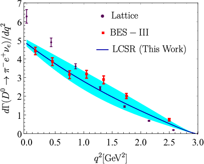
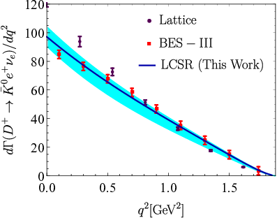
Figure 2: The LCSR predictions for the D→PD\to P decay width, the solid lines represent center values and the shaded bands correspond to their uncertainties. The BES-III ablikim:2017lks results and Lattice Lubicz:2017syv results are also presented as a comparison.
Table 4: The central value of D→PD\to P HFFs at the q2=0​GeV2q^{2}=0~{\rm GeV^{2}} for LO and NLO contributions, respectively.
  𝒫0;tK​(0){\cal P}^{K}_{0;t}(0)   𝒫0;tπ​(0){\cal P}_{0;t}^{\pi}(0)
LO 0.7570.757 0.6750.675
NLO 0.0230.023 0.0130.013
Total 0.7800.780 0.6880.688

Theoretically, the LCSRs for D→PD\to P HFFs are applicable in low and intermediate q2q^{2}-regions, qLCSR,max2≃mc2−2​mc​Eq^{2}_{\rm LCSR,max}\simeq m_{c}^{2}-2m_{c}E. Specifically, with the hadronic scale E≈500​MeVE\approx 500\rm{MeV} Khodjamirian:2000ds, the qLCSR,max2q^{2}_{\rm LCSR,max} can be taken as 0.6​GeV20.6~\rm{GeV}^{2}. While, the allowable physical range is 0≤q2≤qmax2=(mD−mP)20\leq q^{2}\leq q^{2}_{\rm max}=(m_{D}-m_{P})^{2}, i.e. q2∈[0,3.0]​GeV2q^{2}\in[0,3.0]{\rm GeV^{2}} for D→πD\to\pi and q2∈[0,1.88]​GeV2q^{2}\in[0,1.88]{\rm GeV^{2}} for D→KD\to K, respectively. Based on the analyticity and unitarity properties of these HFFs, the extrapolation of these HFFs to the whole physical q2q^{2}-regions can be implemented via a rapidly converging series over the z⁡(t)z(t)-expansion Bharucha:2010im. Specifically, the extrapolation of the HFFs satisfies the following parameterized formula,

𝒫0​(t)\displaystyle{\cal P}_{0}(t) =1B⁡(t)​ϕTP​(t)​∑k=0K−1αk(0)​zk​(t),\displaystyle=\frac{1}{B(t)\,\phi_{T}^{P}(t)}\,\sum_{k=0}^{K-1}\alpha^{(0)}_{k}\,z^{k}(t)\,, (37)
𝒫t​(t)\displaystyle{\cal P}_{t}(t) =1B⁡(t)​z⁡(t,t−)​ϕLP​(t)​∑k=0K−1αk(t)​zk​(t),\displaystyle=\frac{1}{B(t)\,\sqrt{z(t,t_{-})}\,\phi_{L}^{P}(t)}\,\sum_{k=0}^{K-1}\alpha^{(t)}_{k}\,z^{k}(t)\,, (38)

where ϕLP​(t)=ϕTP​(t)=1\phi_{L}^{P}(t)=\phi_{T}^{P}(t)=1, z⁡(t,t−)=λ/mD2\sqrt{z(t,t_{-})}=\sqrt{\lambda}/m_{D}^{2} and

z⁡(t)=t+−t−t+−t0t+−t+t+−t0,\displaystyle z(t)=\frac{\sqrt{t_{+}-t}-\sqrt{t_{+}-t_{0}}}{\sqrt{t_{+}-t}+\sqrt{t_{+}-t_{0}}}, (39)

with t±=(mD±mP)2t_{\pm}=(m_{D}\pm m_{P})^{2} and t0=t+​(1−1−t−/t+)t_{0}=t_{+}(1-\sqrt{1-t_{-}/t_{+}}). The B⁡(t)=1−q2/mR,i2B(t)=1-q^{2}/m_{R,i}^{2} is a simple pole corresponding to the first resonance in the spectrum. The resonance masses of quantum number JPJ^{P} are essential for the parameterisation of D→PD\to P HFFs 𝒫0;tP{\cal P}_{0;t}^{P}  Tanabashi:2018oca; Leljak:2019eyw, i.e.

Fi=𝒫0P,JP=1−,mR,i=2.010​GeV\displaystyle F_{i}={\cal P}_{0}^{P},~~J^{P}=1^{-},~~m_{R,i}=2.010~{\rm GeV} (40)
Fi=𝒫tP,JP=0+,mR,i=2.007​GeV\displaystyle F_{i}={\cal P}_{t}^{P},~~J^{P}=0^{+},~~m_{R,i}=2.007~{\rm GeV}
Table 5: The fitted parameters a0;1;2Pa_{0;1;2}^{P} for the HFFs 𝒫0;tP{\cal P}_{0;t}^{P}, where all input parameters are set to be their central values.
𝒫0π~~{\cal P}_{0}^{\pi}   𝒫tπ{\cal P}_{t}^{\pi}   𝒫0K{\cal P}_{0}^{K}   𝒫tK{\cal P}_{t}^{K}
a0a_{0} 0.672 1.8751.875 0.7620.762 1.8481.848
a1a_{1} −0.354-0.354 0.7080.708 −0.784-0.784 −19.217-19.217
a2a_{2} 2.607 −47.245-47.245 20.72520.725 −50.443-50.443
Δ\Delta 0.00016 0.000220.00022 0.007580.00758 0.000000.00000

The parameters akσa_{k}^{\sigma} can be determined by requiring the “quality” of fit Δ<0.01\Delta<0.01, where Δ\Delta is defined as

Δ=∑t|𝒫σ​(t)−𝒫σfit​(t)|∑t|𝒫σ​(t)|,\Delta=\frac{\sum_{t}\left|{\cal P}_{\sigma}(t)-{\cal P}_{\sigma}^{\rm fit}(t)\right|}{\sum_{t}\left|{\cal P}_{\sigma}(t)\right|}, (41)

where t∈[0,0.06,⋯,0.54,0.6]​GeV2t\in[0,0.06,\cdots,0.54,0.6]~{\rm GeV}^{2}. The determined parameters akρ,σa_{k}^{\rho,\sigma} are listed in Table 5, in which all the input parameters are set to be their central values. We put the extrapolated D→PD\to P HFFs 𝒫σP​(q2){\cal P}_{\sigma}^{P}(q^{2}) in Fig. 1, where the shaded band stands for the squared average of all the mentioned uncertainties. All the HFFs increases with the increase of the squared momentum transfer.

Table 6: Branching fractions of D→P​ℓ+​νℓD\to P\ell^{+}\nu_{\ell} (in unit 10−210^{-2}). The errors are squared averages of all the mentioned error sources. As a comparison, we also present the prediction for various methods.
Channel LCSR(This Work) BES-III ablikim:2017lks CLEO-c Besson:2009 BABAR Lees:2015 Belle Widhalm:2006wz PDG Tanabashi:2018oca CQM Soni:2017eug
D+→K¯0​e+​νeD^{+}\to\bar{K}^{0}e^{+}\nu_{e} 8.547−1.108+0.4458.547^{+0.445}_{-1.108} 8.60(6)(15) 8.83(10)(20) - - - 8.84
D+→K¯0​μ+​νμD^{+}\to\bar{K}^{0}\mu^{+}\nu_{\mu} 8.435−1.100+0.4378.435^{+0.437}_{-1.100} 8.72(7)(18) - - - - 8.60
D+→π0​e+​νeD^{+}\to\pi^{0}e^{+}\nu_{e} 0.328−0.044+0.0560.328^{+0.056}_{-0.044} 0.36(8)(5) 0.405(16)(9) - - - 0.309
D+→π0​μ+​νμD^{+}\to\pi^{0}\mu^{+}\nu_{\mu} 0.325−0.044+0.0560.325^{+0.056}_{-0.044} - - - - - 0.303
D0→K−​e+​νeD^{0}\to K^{-}e^{+}\nu_{e} 3.370−0.437+0.1763.370^{+0.176}_{-0.437} 3.505(14)(33) 3.50(3)(4) - 3.45(7)(20) 3.538(33) 3.46
D0→K−​μ+​νμD^{0}\to K^{-}\mu^{+}\nu_{\mu} 3.325−0.433+0.1723.325^{+0.172}_{-0.433} 3.505(14)(33) - - - 3.33(13) 3.36
D0→π−​e+​νeD^{0}\to\pi^{-}e^{+}\nu_{e} 0.258−0.035+0.0440.258^{+0.044}_{-0.035} 0.295(4)(3) 0.288(8)(3) 0.277(7)(9) 0.255(19)(16) - 0.239
D0→π−​μ+​νμD^{0}\to\pi^{-}\mu^{+}\nu_{\mu} 0.256−0.035+0.0440.256^{+0.044}_{-0.035} - - - - 0.238(24) 0.235

III.3 The semi-leptonic decay processes of DD-meson

The differential decay rate for the process involving pseudoscalar mesons D→PD\to P is given by Zhong:2018exo

d​Γd​q2(D→Pℓν¯ℓ)=GF2​|Vc​q|224​π3​mD2(1−2δℓ)2|p→P|[(1+δℓ)\displaystyle\frac{d\Gamma}{dq^{2}}(D\to P\ell\bar{\nu}_{\ell})=\frac{G_{F}^{2}|V_{cq}|^{2}}{24\pi^{3}m_{D}^{2}}(1-2\delta_{\ell})^{2}|\vec{p}_{P}|\bigg[(1+\delta_{\ell})
×mD2|p→P|2|𝒫0P(q2)|2+3​λ​δℓ4|𝒫tP(q2)|2],\displaystyle\quad\times m_{D}^{2}|\vec{p}_{P}|^{2}\big|{\cal P}_{0}^{P}(q^{2})\big|^{2}+\frac{3\lambda\delta_{\ell}}{4}\big|{\cal P}_{t}^{P}(q^{2})\big|^{2}\bigg], (42)

with δℓ=mℓ2/(2​q2)\delta_{\ell}=m_{\ell}^{2}/(2q^{2}), |p→P||\vec{p}_{P}| is three-momentum of the pseudoscalar mesons in the DD-meson rest frame, the fermi coupling constant GF=1.166×10⁻⁵​GeV−2{G_{F}}=1.166\times 10^{-5}{\rm GeV^{-2}}, |Vc​s|=0.944|V_{cs}|=0.944 and |Vc​d|=0.2155|V_{cd}|=0.2155 Chen:2018zsn.

After taking the resultant HFFs and other input parameters into Eq. (42), we can obtain the differential decay widths of D→P​ℓ​νℓD\to P\ell\nu_{\ell} in the entire kinematical range of squared momentum transfer, which is shown in Fig. 2. Where the solid lines represent center values and the shaded bands correspond to their uncertainties. The BES-III collaboration ablikim:2017lks and Lattice Lubicz:2017syv results are also presented as a comparison. As the suppression of the factor |p→P|=λ/(2​mD)|\vec{p}_{P}|=\sqrt{\lambda}/(2m_{D}) in the decay width formula for the D→P​ℓ​ν¯ℓD\to P\ell\bar{\nu}_{\ell} semilepton decay, the differential decay width monotonously decreases with the increment of q2q^{2}, which is clearly illustrated in Fig. 2. More specifically, comparing with the decreasing rate of differential decay width for BES-III, our predictions are almost identical with it, so our results agree with the BES-III measurements within errors.

As a further step, the branching fractions of D→P​ℓ+​νℓD\to P\ell^{+}\nu_{\ell} can be obtain by employing τ​(D0)=0.410​(2)​ps\tau({D^{0}})=0.410(2)~{\rm ps} and τ⁡(D+)=1.040​(7)​ps\tau({D^{+}})=1.040(7)~{\rm ps} and making integration with squared momentum transfer, the results are collected in Table 6. The relevant experiment results BES-III ablikim:2017lks, CLEO-c Besson:2009, PDG Tanabashi:2018oca, Belle Widhalm:2006wz, BABAR Lees:2015 and theory results the covariant quark model (CQM) Soni:2017eug are also presented as a comparison. Our results on the branching fractions for D→π​ℓ+​ν¯ℓD\to\pi\ell^{+}\bar{\nu}_{\ell} and D→K​ℓ+​ν¯ℓD\to K\ell^{+}\bar{\nu}_{\ell} are consistent with the BES-III measurements within errors. Compared with the CQM theoretical predictions for the D+→π0​ℓ+​νℓD^{+}\to\pi^{0}\ell^{+}\nu_{\ell} channel, our results are closer to the experimental results.

Refer to caption
Refer to caption
Refer to caption
Refer to caption
Refer to caption
Refer to caption
Refer to caption
Refer to caption
Figure 3: The forward-backward asymmetries and the convexity parameters of the decays D→π​ℓ+​νℓD\to\pi\ell^{+}\nu_{\ell} and D→K​ℓ+​νℓD\to K\ell^{+}\nu_{\ell} with ℓ=e,μ\ell=e,\mu, the shaded bands corresponds to the uncertainties from theoretical input parameters.

Furthermore, the ratio for branching fractions for the different lepton channel are defined as, RP=Γ⁡(D→P​μ+​νμ)/Γ⁡(D→P​e+​νe).R_{P}={\Gamma(D\to P\mu^{+}\nu_{\mu})}/{\Gamma(D\to Pe^{+}\nu_{e})}. After taking the D→P​ℓ+​νℓD\to P\ell^{+}\nu_{\ell} decay width into the above equation and replacing HFFs with Eqs. (20) and (21), we can get ratios of semileptonic bractions as follows:

Rπ0\displaystyle R_{\pi^{0}} =Γ⁡(D+→π0​μ+​νμ)Γ⁡(D+→π0​e+​νe)=0.991−0.197+0.230\displaystyle=\frac{\Gamma(D^{+}\to\pi^{0}\mu^{+}\nu_{\mu})}{\Gamma(D^{+}\to\pi^{0}e^{+}\nu_{e})}=0.991^{+0.230}_{-0.197}
Rπ−\displaystyle R_{\pi^{-}} =Γ⁡(D0→π−​μ+​νμ)Γ⁡(D0→π−​e+​νe)=0.992−0.198+0.231\displaystyle=\frac{\Gamma(D^{0}\to\pi^{-}\mu^{+}\nu_{\mu})}{\Gamma(D^{0}\to\pi^{-}e^{+}\nu_{e})}=0.992^{+0.231}_{-0.198}
RK¯0\displaystyle R_{\bar{K}^{0}} =Γ⁡(D+→K¯0​μ+​νμ)Γ⁡(D+→K¯0​e+​νe)=0.987−0.138+0.156\displaystyle=\frac{\Gamma(D^{+}\to\bar{K}^{0}\mu^{+}\nu_{\mu})}{\Gamma(D^{+}\to\bar{K}^{0}e^{+}\nu_{e})}=0.987^{+0.156}_{-0.138}
RK−\displaystyle R_{K^{-}} =Γ⁡(D0→K−​μ+​νμ)Γ⁡(D0→K−​e+​νe)=0.987−0.138+0.156\displaystyle=\frac{\Gamma(D^{0}\to K^{-}\mu^{+}\nu_{\mu})}{\Gamma(D^{0}\to K^{-}e^{+}\nu_{e})}=0.987^{+0.156}_{-0.138} (43)

The above ratios of our calculation are consistent with the CQM predictions RK¯0CQM=0.97R_{\bar{K}^{0}}^{\rm CQM}=0.97 Soni:2017eug, which are more close to 11.

Moreover, the obtained HFFs can be used to calculate the forward-backward asymmetry 𝒜FB​(q2){\cal A}_{\rm FB}(q^{2}), which can be expressed as follows:

𝒜FBℓ​(q2)=3​δℓ​𝒫0P​(q2)​𝒫tP​(q2)(1+δℓ)​|𝒫0P​(q2)|2+3​|𝒫tP​(q2)|2\displaystyle{\cal A}_{\rm FB}^{\ell}(q^{2})=\frac{3\delta_{\ell}{\cal P}_{0}^{P}(q^{2}){\cal P}_{t}^{P}(q^{2})}{(1+\delta_{\ell})|{\cal P}_{0}^{P}(q^{2})|^{2}+3|{\cal P}_{t}^{P}(q^{2})|^{2}} (44)

Also, the lepton side convexity parameter 𝒞Fℓ​(q2){\cal C}_{F}^{\ell}(q^{2}) can be written as:

𝒞Fℓ​(q2)=−32​(1−2​δℓ)​|𝒫0P​(q2)|2(1+δℓ)​|𝒫0P​(q2)|2+3​δℓ​|𝒫tP​(q2)|2,\displaystyle{\cal C}_{F}^{\ell}(q^{2})=-\frac{3}{2}\frac{(1-2\delta_{\ell})|{\cal P}_{0}^{P}(q^{2})|^{2}}{(1+\delta_{\ell})|{\cal P}_{0}^{P}(q^{2})|^{2}+3\delta_{\ell}|{\cal P}_{t}^{P}(q^{2})|^{2}}, (45)

After taking the HFFs into Eqs. (44) and (45), we present the forward-backward asymmetry and the lepton convexity parameter within uncertainties in Fig. 3. Finally, we list our the mean values for forward-backward asymmetry ⟨𝒜FBℓ⟩\langle{\cal A}_{\rm FB}^{\ell}\rangle, lepton convexity parameter ⟨𝒞Fℓ⟩\langle{\cal C}_{F}^{\ell}\rangle in the Table 7. It is seen that, for both D→π​ℓ​ν¯ℓD\to\pi\ell\bar{\nu}_{\ell} and D→K​ℓ​ν¯ℓD\to K\ell\bar{\nu}_{\ell} decay transitions, ⟨𝒜FBμ⟩\langle{\cal A}_{\rm FB}^{\mu}\rangle are about 10510^{5} times larger than ⟨𝒜FBe⟩\langle{\cal A}_{\rm FB}^{e}\rangle, while ⟨𝒞Fμ⟩\langle{\cal C}_{F}^{\mu}\rangle is a little larger than ⟨𝒞Fe⟩\langle{\cal C}_{F}^{e}\rangle. For the D→P​ℓ​νℓD\to P\ell\nu_{\ell}, our predictions are different from the CQM results Soni:2017eug. Consider formula Eqs. (44) and (45) refer to HFFs, these differences may provide a way to test those HFFs in future experiments.

Table 7: The forward-backward asymmetry and lepton convexity parameter. The errors are squared averages of all the mentioned error sources.
 Channel   ⟨𝒜FBℓ⟩\langle{\cal A}_{\rm FB}^{\ell}\rangle(This work)   ⟨𝒞Fℓ⟩\langle{\cal C}_{F}^{\ell}\rangle (This work)    ⟨𝒜FBℓ⟩\langle{\cal A}_{\rm FB}^{\ell}\rangle (CQM) Soni:2017eug   ⟨𝒞Fℓ⟩\langle{\cal C}_{F}^{\ell}\rangle (CQM) Soni:2017eug
D→π​e+​νeD\to\pi e^{+}\nu_{e} (−4.827−1.247+0.947)×10−6\big(-4.827^{+0.947}_{-1.247}\big)\times 10^{-6} −4.425−0.000+0.000-4.425^{+0.000}_{-0.000} −4.1×10⁻⁶-4.1\times 10^{-6} −1.5-1.5
D→π​μ+​νμD\to\pi\mu^{+}\nu_{\mu} −0.155−0.017+0.013-0.155^{+0.013}_{-0.017} −3.303−0.509+0.396-3.303^{+0.396}_{-0.509} −0.04-0.04 −1.37-1.37
D→K​e+​νeD\to Ke^{+}\nu_{e} (−4.564−1.310+0.316)×10−6\big(-4.564^{+0.316}_{-1.310}\big)\times 10^{-6} −2.775−0.000+0.000-2.775^{+0.000}_{-0.000} −4.27×10⁻⁶-4.27\times 10^{-6} −1.5-1.5
D→K​μ+​νμD\to K\mu^{+}\nu_{\mu} −0.123−0.015+0.003-0.123^{+0.003}_{-0.015} −1.866−0.274+0.063-1.866^{+0.063}_{-0.274} −0.058-0.058 −1.32-1.32

IV Summary

In this paper, we investigate the D→PD\to P HFFs 𝒫σP​(q2){\cal P}_{\sigma}^{P}(q^{2}) with σ=0,t\sigma=0,t within LCSR approach up to NLO gluon radiation correction for twist-2 contributions accuracy. At large recoil point q2↝0​GeV2q^{2}\rightsquigarrow 0~{\rm GeV^{2}}, we have 𝒫t,0π​(0)=0.688−0.024+0.020{\cal P}_{t,0}^{\pi}(0)=0.688^{+0.020}_{-0.024}, 𝒫t,0K​(0)=0.780−0.029+0.024{\cal P}_{t,0}^{K}(0)=0.780^{+0.024}_{-0.029}. The detailed uncertainties of these predictions caused by the errors of the input parameters are given in Table 3. Then, contributions of the LO and NLO to the LCSR results are given in Table 4,and the maximal contribution of NLO for 𝒫0,tP​(0){\cal P}_{0,t}^{P}(0) are no more than 3%3\%. The results indicate those HFFs keep a high-accurate and the predictions we make with it are credible.

After extrapolating the D→PD\to P HFFs to whole physical q2q^{2}-region, the behavior of these HFFs within uncertainties are present in Fig 1. Furthermore, we apply these HFFs to study the semilepton decays processes D→P​ℓ​νℓD\to P\ell\nu_{\ell}. For the decay width in Fig. 2, our results agree with BES-III collaboration within errors, especially in the low q2q^{2} regions. With the help of DD-meson lifetime, the two types of branching ratios are obtained and listed in Table 6. Our predictions are in good agreement with the BES-III and other experimental results, which provides a better prediction of the D→π​ℓ​νℓD\to\pi\ell\nu_{\ell} decay process than that of the CQM Soni:2017eug. Meanwhile, we list the ratio of branching fraction with different lepton channel RPR_{P} in Eq. (43), which shows that RK¯0=RK−R_{\bar{K}^{0}}=R_{K^{-}} and all values of these ratios close to 1.

As a further step, by taking the D→PD\to P HFFs into the forward-backward asymmetry 𝒜FBℓ​(q2){\cal A}_{\rm FB}^{\ell}(q^{2}) and the lepton convexity parameter 𝒞Fℓ​(q2){\cal C}_{F}^{\ell}(q^{2}), we give these two observable in Fig. 3. Meanwhile, the mean values for the forward-backward asymmetry ⟨𝒜FBℓ⟩\langle{\cal A}_{\rm FB}^{\ell}\rangle and lepton convexity parameter ⟨𝒞Fℓ⟩\langle{\cal C}_{F}^{\ell}\rangle are listed in Table 7. The table shows that ⟨𝒜FBμ⟩\langle{\cal A}_{\rm FB}^{\mu}\rangle are about 10510^{5} times larger than ⟨𝒜FBe⟩\langle{\cal A}_{\rm FB}^{e}\rangle. There is a wide difference between our result and the CQM for both ⟨𝒜FBℓ⟩\langle{\cal A}_{\rm FB}^{\ell}\rangle and ⟨𝒞Fℓ⟩\langle{\cal C}_{F}^{\ell}\rangle for the D→P​ℓ​νℓD\to P\ell\nu_{\ell} decay. The discrepancy may provide a way to test those HFFs in future experiments.

Acknowledgments

We are grateful to Prof. Xing-Gang Wu and Tao Zhong for many helpful discussions and suggestions. This work was supported in part by the National Science Foundation of China under Grant No.11765007, the National Natural Science Foundation of China under Grant No.11947302, the Project of Guizhou Provincial Department of Science and Technology under Grant No.KY[2017]1089 and No.KY[2019]1171, the China Postdoctoral Science Foundation under Grant No.2019TQ0329.

References

  • (1) J. Adler et al., Search for the Decay D+→μ+​νμD^{+}\to\mu^{+}\nu_{\mu} and an Upper Limit on the Pseudoscalar Decay Constant, Phys. Rev. Lett. 60, 1375 (1988).
  • (2) B. I. Eisenstein et al. [CLEO Collaboration], Precision Measurement of B⁡(D+→μ+ν)B(D^{+}\to\mu+\nu) and the Pseudoscalar Decay Constant f⁡(D+)f(D^{+}), Phys. Rev. D78, 052003 (2008).
  • (3) M. Artuso et al. [CLEO Collaboration], Improved measurement of B⁡(D+→μ+​ν)B(D^{+}\to\mu^{+}\nu) and the pseudoscalar decay constant f⁡(D+)f(D^{+}), Phys. Rev. Lett. 95, 251801 (2005).
  • (4) G. Bonvicini et al. [CLEO Collaboration], Measuring B⁡(D+→μ+​ν)B(D^{+}\to\mu^{+}\nu) and the pseudoscalar decay constant f⁡(D+)f(D^{+}), Phys. Rev. D70, 112004 (2004).
  • (5) M. Ablikim et al. [BES Collaboration], Direct measurement of the pseudoscalar decay constant f⁡(D+)f(D^{+}), Phys. Lett. B610, 183 (2005).
  • (6) J. Adler et al. [MARK-III Collaboration], Measurement of the Branching Fractions for D0→π−​e+​νeD^{0}\to\pi^{-}e^{+}\nu_{e} and D0→K−​e+​νeD^{0}\to K^{-}e^{+}\nu_{e} and Determination of (Vc​d/Vc​s)2(V_{cd}/V_{cs})^{2}, Phys. Rev. Lett. 62, 1821 (1989).
  • (7) L. Widhalm et al. [Belle Collaboration], Measurement of D0→π​ℓ​ν​(K​ℓ​ν)D^{0}\to\pi\ell\nu(K\ell\nu) Form Factors and Absolute Branching Fractions, Phys. Rev. Lett. 97, 061804 (2006).
  • (8) D. Besson et al. [CLEO Collaboration], Improved measurements of DD meson semileptonic decays to π\pi and KK mesons, Phys. Rev. D80, 032005 (2009).
  • (9) J. P. Lees et al. [BABAR Collaboration], Measurement of the D0→π−​e+​νeD^{0}\to\pi^{-}e^{+}\nu_{e} differential decay branching fraction as a function of q2q^{2} and study of form factor parameterizations, Phys. Rev. D91, 052022 (2015).
  • (10) M. Ablikim et al. [BES-III Collaboration], Study of Dynamics of D0→K−​e+​νeD^{0}\to K^{-}e^{+}\nu_{e} and D0→π−​e+​νeD^{0}\to\pi^{-}e^{+}\nu_{e} Decays, Phys. Rev. D92, 072012 (2015).
  • (11) M. Ablikim et al. [BES-III Collaboration], Improved measurement of the absolute branching fraction of D+→K¯0​μ+​νμD^{+}\rightarrow\bar{K}^{0}\mu^{+}\nu_{\mu}, Eur. Phys. J. C76, 369 (2016).
  • (12) M. Ablikim et al. [BES-III Collaboration], Study of decay dynamics and C​PCP asymmetry in D+→KL0​e+​νeD^{+}\to K^{0}_{L}e^{+}\nu_{e} decay, Phys. Rev. D92, 112008 (2015).
  • (13) M. Ablikim et al. [BES-III Collaboration], First Measurement of the Form Factors in Ds+→K0​e+​νeD^{+}_{s}\rightarrow K^{0}e^{+}\nu_{e} and Ds+→K∗0​e+​νeD^{+}_{s}\rightarrow K^{*0}e^{+}\nu_{e} Decays, Phys. Rev. Lett. 122, 061801 (2019).
  • (14) J. Koponen et al. [HPQCD Collaboration], D→KD\to K and D→πD\to\pi semileptonic form factors from Lattice QCD, arXiv:1208.6242 [hep-lat].
  • (15) M. Ablikim et al. [BES-III Collaboration], Phys. Rev. D96, 012002 (2017)
  • (16) Y. Amhis et al. [HFLAV Collaboration], Averages of bb-hadron, cc-hadron, and τ\tau-lepton properties as of summer 2016, Eur. Phys. J. C77, 895 (2017).
  • (17) R. N. Faustov, V. O. Galkin and X. W. Kang, Semileptonic decays of DD and DsD_{s} mesons in the relativistic quark model, Phys. Rev. D 101 (2020) 013004.
  • (18) S. H. Zhou and C. D. Lü, Extraction of the CKM phase γ\gamma from charmless two-body BB meson decays,” arXiv:1910.03160 [hep-ph].
  • (19) J. Charles et al. [CKMfitter Group], CP violation and the CKM matrix: Assessing the impact of the asymmetric BB factories, Eur. Phys. J. C41, 1 (2005).
  • (20) N. G. Deshpande, B. Dutta and S. Oh, Branching ratios and CP asymmetries of BB decays to a vector and a pseudoscalar meson, Phys. Lett. B473, 141 (2000).
  • (21) M. A. Shifman, A. I. Vainshtein and V. I. Zakharov, QCD and Resonance Physics. Theoretical Foundations, Nucl. Phys. B147, 385 (1979).
  • (22) P. Ball and V. M. Braun, Use and misuse of QCD sum rules in heavy to light transitions: The Decay B→ρ​eB\to\rho e neutrino reexamined, Phys. Rev. D55, 5561 (1997).
  • (23) P. Ball and R. Zwicky, B(d​s)→ρB_{(ds)}\to\rho, ω\omega, K∗K^{*}, ϕ\phi decay form-factors from light-cone sum rules revisited, Phys. Rev. D71, 014029 (2005).
  • (24) T. Huang, Z. H. Li, X. G. Wu and F. Zuo, Semileptonic B⁡(Bs,Bc)B(B_{s},B_{c}) decays in the light-cone QCD sum rules, Int. J. Mod. Phys. A23, 3237 (2008).
  • (25) A. Khodjamirian, T. Mannel, A. A. Pivovarov and Y. M. Wang, Charm-loop effect in B→K∗​ℓ+​ℓ−B\to K^{*}\ell^{+}\ell^{-} and B→K∗​γB\to K^{*}\gamma, JHEP1009, 089 (2010).
  • (26) M. Ahmady, R. Campbell, S. Lord and R. Sandapen, Predicting the B→ρB\to\rho form factors using AdS/QCD Distribution Amplitudes for the ρ\rho meson, Phys. Rev. D88, 074031 (2013).
  • (27) A. Bharucha, D. M. Straub and R. Zwicky, B→V​ℓ+​ℓ−B\to V\ell^{+}\ell^{-} in the Standard Model from light-cone sum rules, JHEP 1608, 098 (2016).
  • (28) H. B. Fu, X. G. Wu, H. Y. Han, Y. Ma and H. Y. Bi, The ρ\rho-meson longitudinal leading-twist distribution amplitude, Phys. Lett. B738, 228 (2014).
  • (29) W. Cheng, X. G. Wu and H. B. Fu, Reconsideration of the B→K∗B\to K^{*} transition form factors within the QCD light-cone sum rules, Phys. Rev. D95, 094023 (2017).
  • (30) Y. M. Wang and Y. L. Shen, “QCD corrections to B¡ú¦Ð form factors from light-cone sum rules,” Nucl. Phys. B 898, 563-604 (2015).
  • (31) H. N. Li, Y. L. Shen and Y. M. Wang, “Next-to-leading-order corrections to B→πB\to\pi form factors in kTk_{T} factorization,” Phys. Rev. D85, 074004 (2012).
  • (32) H. N. Li, Y. L. Shen and Y. M. Wang, “Resummation of rapidity logarithms in BB meson wave functions,” JHEP 02, 008 (2013).
  • (33) J. M. Flynn et al. [UKQCD Collaboration], Lattice study of the decay B¯0→ρ+​l−​νl¯\bar{B}^{0}\to\rho^{+}l^{-}\bar{\nu_{l}}: Model independent determination of |Vu​b||V_{ub}|, Nucl. Phys. B461, 327 (1996).
  • (34) L. Del Debbio et al. [UKQCD Collaboration], Lattice constrained parametrizations of form-factors for semileptonic and rare radiative BB decays, Nucl. Phys. Proc. Suppl. 63, 383 (1998).
  • (35) K. C. Bowler et al. [UKQCD Collaboration], B→ρ​ℓ​νB\to\rho\ell\nu form-factors in lattice QCD, JHEP 0405, 035 (2004).
  • (36) R. R. Horgan, Z. F. Liu, S. Meinel and M. Wingate, Lattice QCD calculation of form factors describing the rare decays B→K∗​ℓ+​ℓ−B\to K^{*}\ell^{+}\ell^{-} and Bs→ϕ​ℓ+​ℓ−B_{s}\to\phi\ell^{+}\ell^{-}, Phys. Rev. D89, 094501 (2014).
  • (37) R. R. Horgan, Z. Liu, S. Meinel and M. Wingate, Calculation of B0→K∗0​μ+​μ−B^{0}\to K^{*0}\mu^{+}\mu^{-} and Bs0→ϕ​μ+​μ−B_{s}^{0}\to\phi\mu^{+}\mu^{-} observables using form factors from lattice QCD, Phys. Rev. Lett. 112, 212003 (2014).
  • (38) A. Agadjanov, V. Bernard, U. G. Meibner and A. Rusetsky, The B→K∗B\to K^{*} form factors on the lattice, Nucl. Phys. B910, 387 (2016).
  • (39) T. Kurimoto, H. n. Li and A. I. Sanda, Leading power contributions to B→π,ρB\to\pi,\rho transition form-factors, Phys. Rev. D65, 014007 (2002).
  • (40) C. H. Chen and C. Q. Geng, Analysis of B →\to K∗​ℓ+​ℓ−K^{*}\ell^{+}\ell^{-} decays at large recoil region, Nucl. Phys. B636, 338 (2002).
  • (41) T. Kurimoto, H. n. Li and A. I. Sanda, B→D(∗)B\to D^{(*)} form-factors in perturbative QCD, Phys. Rev. D67, 054028 (2003).
  • (42) Y. Y. Keum, M. Matsumori and A. I. Sanda, CP asymmetry, branching ratios and isospin breaking effects of B→K∗​γB\to K^{*}\gamma with perturbative QCD approach, Phys. Rev. D72, 014013 (2005).
  • (43) Y. Y. Fan, W. F. Wang, S. Cheng and Z. J. Xiao, Semileptonic decays B→D(∗)​l​νB\to D^{(*)}l\nu in the perturbative QCD factorization approach, Chin. Sci. Bull. 59, 125 (2014).
  • (44) J. Gao, C. D. Lü, Y. L. Shen, Y. M. Wang and Y. B. Wei, Precision calculations of B→VB\to V form factors in QCD, arXiv:1907.11092 [hep-ph].
  • (45) C. D. Lü, Y. L. Shen, Y. M. Wang and Y. B. Wei, QCD calculations of B→π,KB\to\pi,K form factors with higher-twist corrections, JHEP 1901 (2019) 024
  • (46) C. D. Lü, W. Wang, Y. Xing and Q. A. Zhang, Perturbative QCD analysis of exclusive processes e+​e−→V​Pe^{+}e^{-}\rightarrow VP and e+​e−→T​Pe^{+}e^{-}\rightarrow TP, Phys. Rev. D97, 114016 (2018).
  • (47) A. Bharucha, T. Feldmann and M. Wick, Theoretical and Phenomenological Constraints on Form Factors for Radiative and Semi-Leptonic BB-Meson Decays, JHEP 1009, 090 (2010).
  • (48) W. Cheng, X. G. Wu, R. Y. Zhou and H. B. Fu, The B→ρB\to\rho helicity form factors within the QCD light-cone sum rules, Phys. Rev. D98, 096013 (2018).
  • (49) P. Ball and R. Zwicky, New results on B→π,K,ηB\to\pi,K,\eta decay formfactors from light-cone sum rules, Phys. Rev. D71, 014015 (2005)
  • (50) G. Duplancic, A. Khodjamirian, T. Mannel, B. Melic and N. Offen, Light-cone sum rules for B→πB\to\pi form factors revisited, JHEP 0804, 014 (2008).
  • (51) Z. H. Li, Z. G. Si, Y. Wang and N. Zhu, B→πB\to\piℓ+​ℓ−{\ell}^{+}{\ell}^{-} form factors reexamined in the whole kinematically accessible region, Nucl. Phys. B900 (2015) 198.
  • (52) C. Patrignani et al. [Particle Data Group], Review of Particle Physics, Chin. Phys. C 40 (2016) no.10, 100001.
  • (53) A. Khodjamirian, C. Klein, T. Mannel and N. Offen, Semileptonic charm decays D→π​ℓ​νℓD\to\pi\ell\nu_{\ell} and D→K​ℓ​νℓD\to K\ell\nu_{\ell} from QCD Light-Cone Sum Rules, Phys. Rev. D 80 (2009) 114005.
  • (54) M. Tanabashi et al. [Particle Data Group], Review of Particle Physics, Phys. Rev. D98 (2018) 030001.
  • (55) H. B. Fu, L. Zeng, R. Lü, W. Cheng and X. G. Wu, The D→ρD\to\rho transition form factors within the QCD light-cone sum rules and the DD-meson semileptonic decays D0→ρ−​e+​νeD^{0}\to\rho^{-}e^{+}\nu_{e} and D+→ρ0​e+​νeD^{+}\to\rho^{0}e^{+}\nu_{e}, arXiv:1808.06412 [hep-ph].
  • (56) P. Ball, V. M. Braun and A. Lenz, Higher-twist distribution amplitudes of the KK meson in QCD, JHEP 0605 (2006) 004.
  • (57) A. Khodjamirian, R. Ruckl, S. Weinzierl, C. W. Winhart and O. I. Yakovlev, Predictions on B→π​l¯​νlB\to\pi\bar{l}\nu_{l}, D→π​l¯​νlD\to\pi\bar{l}\nu_{l} and D→K​l¯​νlD\to K\bar{l}\nu_{l} from QCD light cone sum rules, Phys. Rev. D62 (2000) 114002.
  • (58) D. Leljak, B. Melic and M. Patra, On lepton flavour universality in semileptonic Bc→ηc,J/ψB_{c}\to\eta_{c},J/\psi decays, JHEP 1905 (2019) 094.
  • (59) T. Zhong, Y. Zhang, X. G. Wu, H. B. Fu and T. Huang, The ratio ℛ⁡(D)\mathcal{R}(D) and the DD-meson distribution amplitude, Eur. Phys. J. C78, 937 (2018).
  • (60) J. Chen [BES-III Collaboration], Charm Leptonic and semi-Leptonic decays at BES-III, arXiv:1812.00406 [hep-ex].
  • (61) V. Lubicz et al. [ETM], Scalar and vector form factors of D→π⁡(K)​ℓ​νD\to\pi(K)\ell\nu decays with Nf=2+1+1N_{f}=2+1+1 twisted fermions, Phys. Rev. D 96, no.5, 054514 (2017)
  • (62) N. R. Soni and J. N. Pandya, Decay D→K(∗)​ℓ+​νℓ{\mathit{D}\to}{{\mathit{K}}^{(*)}}{{\mathit{\ell}}^{+}}{{\mathit{\nu}}_{{{{\mathit{\ell}}}}}} in covariant quark model, Phys. Rev. D96 (2017) 016017.