Exceptional band touching for strongly correlated systems in equilibrium

In the above, we have seen that a non-Hermitian matrix may show EPs which are characterized by the vorticity (7). In this section, we see that a non-Hermitian matrix governs the single-particle excitation spectrum of correlated systems in equilibrium (i.e., the energy is conserved).

Firstly, we define the retarded single-particle Green’s function $G^{R}(t,\bm{k})$ whose imaginary part corresponds to the single-particle spectrum:

where $\hat{c}^{\dagger}_{\bm{k}\alpha}$ creates a fermion with momentum $\bm{k}$ in the state $\alpha$ (spin, orbital etc.). $\langle{\,}\cdot{\,}\rangle$ denotes the expectation value for temperature $\beta^{-1}$ [$\langle{\,}\cdot{\,}\rangle:=\mathrm{tr}({\,}\cdot{\,}e^{-\beta\hat{H}})$]. $\hat{c}^{\dagger}_{\bm{k}\alpha}(t):=e^{i\hat{H}t}\hat{c}^{\dagger}_{\bm{k}\alpha}e^{-i\hat{H}t}$ with the second quantized Hamiltonian $\hat{H}$ describing the correlated system in equilibrium (i.e., $\hat{H}$ is a Hermitian operator). $\theta(t)$ takes $0$, $1/2$, and $1$ for $t<0$, $t=0$, and $t>0$, respectively. Applying the Fourier transformation, we obtain the Dyson’s equation Abrikosov et al. 2012:

which defines the self-energy $\Sigma(\omega+i\delta,\bm{k})$. Here, $g(\omega+i\delta,\bm{k})$ denotes the retarded Green’s function for free fermions. $\delta$ is an infinitesimal constant ($\delta>0$). With the Green’s function, the single-particle spectral function is defined as $A(\omega,\bm{k})=-\mathrm{Im}\sum_{\alpha}G_{\alpha\alpha}(\omega+i\delta,\bm{k})/\pi$, which can be rewritten as

Here, the matrix $h(\bm{k})$ is the Bloch Hamiltonian for free fermions with momentum $\bm{k}$. 1l denotes the identity matrix. We note that the self-energy $\Sigma(\omega+i\delta,\bm{k})$ is a non-Hermitian matrix, describing the lifetimes of quasi-particles. Therefore, Eq. (14a) indicates that the single-particle excitations of energy $\omega$ are governed by the non-Hermitian matrix $H_{\mathrm{eff}}(\omega,\bm{k})$.

In addition to EPs, the non-Hermiticity of the effective Hamiltonian yields low energy excitations. The energy gap can be pure imaginary because of the non-Hermiticity of $H_{\mathrm{eff}}$. In this case, even when the Bloch Hamiltonian is gapped, the system may show Fermi arcs connecting EPs.

We finish this section by making a comment on an additional condition for the EPs in the single-particle spectrum. The effective Hamiltonian appears in the denominator of the spectral weight (14a), meaning that the EPs are seriously smeared when the denominator is large. Therefore, in order for EPs to emerge as a peak in the single-particle spectral function, the frequency $\omega$ should satisfy an additional condition [for instance see Eq. (19a)].

In this section, we demonstrate that EPs emerge in the single-particle spectrum of a heavy-fermion system, by employing the DMFT. In particular, we analyze the Kondo lattice in two dimensions. The Hamiltonian reads,

where $\hat{c}^{\dagger}_{i\alpha s}$ creates an electron with spin $s=\uparrow,\downarrow$ in orbital $\alpha=a,b$ of site $i$. $\hat{\bm{s}}_{ib}:=\frac{1}{2}\hat{c}^{\dagger}_{ibs}\bm{\sigma}_{ss^{\prime}}\hat{c}_{ibs^{\prime}}$ with the Pauli matrices $\sigma$’s acting on the spin space. $\hat{\bm{S}}$ is the spin $1/2$ operator for the localized spins. Here, the Kondo coupling of electrons in orbital $a$ is neglected for simplicity. The hopping $t_{i\alpha,j\beta}$ is defined so that the Bloch Hamiltonian is written as

where $\epsilon_{0}$, $t$, and $t^{\prime}$ take real values, respectively. The Pauli matrices $\tau$’s act on the orbital space. In the non-interacting case, this model shows two Dirac cones for $t=1$ and $0<\epsilon_{0}<4$.

In order to analyze the above correlated electron system, we employ the DMFT Metzner and Vollhardt 1989; Müller-Hartmann 1989; Georges and Kotliar 1992; Georges et al. 1996 which treats local correlation exactly. In the DMFT framework, the lattice model is mapped to an effective impurity model where the self-energy of spin $s$ $[\Sigma_{s}(\omega+i\delta):=\mathrm{diag}\left(\begin{array}[]{cc}0,&\Sigma_{bs}(\omega+i\delta)\end{array}\right)]$ is computed self-consistently DMF. Here, $\Sigma_{bs}(\omega+i\delta)$ denotes the self-energy for orbital $b$ and spin $s$. In order to compute the self-energy for the effective impurity model, we employ the numerical renormalization group method (NRG) Wilson 1975; Peters et al. 2006; Bulla et al. 2008. This method directly provides the single-particle spectral function, while other methods based on Monte Carlo calculations Hirsch and Fye 1986; Werner et al. 2006; Werner and Millis 2006 require the analytic continuation.

Once the self-energy is obtained, the single-particle spectrum is obtained as

Here, we have omitted the subscript $s$ [$\Sigma(\omega+i\delta):=\mathrm{diag}\left(\begin{array}[]{cc}0,&\Sigma_{b}(\omega+i\delta)\end{array}\right)$] by assuming that the system is in the paramagnetic phase. We note that the effective Hamiltonian is a $2\times 2$ matrix. Expanding it with the Pauli matrices as Eq. (1), we obtain the following coefficients

Therefore, the conditions for EPs appearing as the peak of the single-particle spectral function are written as

Here, the second and the third equations are obtained from Eq. (3), specifying the position of the EP $\bm{k}_{0}$ in the BZ. The first equation specifies the energy $\omega_{0}$ where the EPs emerge as peaks of the spectral function. We note that in the DMFT framework, the momentum dependence of the self-energy is neglected. However, the EPs should emerge even in calculations beyond the DMFT framework because they are topologically protected.

Let us now analyze the Kondo lattice model (15). In the rest of this section, we set the parameters to $\left(\begin{array}[]{ccc}t,&t^{\prime},&\epsilon_{0}\end{array}\right)=\left(\begin{array}[]{ccc}1,&0.667,&0.667\end{array}\right)$. The obtained phase diagram is shown in Fig. 2. When the Kondo coupling is small, an anti-ferromagnetic phase emerges because the Ruderman-Kittel-Kasuya-Yosida interaction Ruderman and Kittel 1954; Kasuya 1956; Yosida 1957 becomes dominant. Increasing the interaction $J$, itinerant electrons and localized spins form singlets due to the Kondo effect. As a result, the anti-ferromagnetic phase is suppressed in the region of strong $J$.

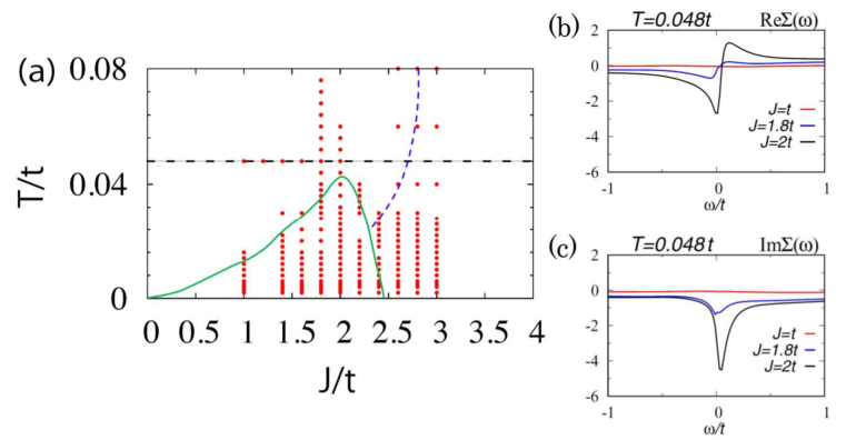
We numerically observe the EPs in the paramagnetic phase. The Kondo effect plays an important role for the emergence of EPs. The self-energy is shown in Figs. 2(b) and 2(c) for $T=0.048t$ which corresponds to the horizontal line in Fig. 2(a). For small $J$ ($J=t$), the real and imaginary parts of the self-energy take small values because the electrons are almost decoupled from the localized spins. Increasing the coupling $J$ enhances the Kondo effect, which results in a dip structure of $\mathrm{Im}\Sigma_{b}(\omega+i\delta)$ in the low-energy region (i.e., around $\omega\sim 0$). This dip structure of the self-energy induces the EPs. The single-particle spectral function for $J=1.8t$ is plotted in Fig. 3. Firstly, we show the data obtained by assuming that the imaginary part of the self-energy is zero [see Fig. 3(a)] in order to show that the imaginary part of the self-energy is essential for the EPs. In this figure, we can see a single peak due to the existence of a Dirac cone. Fig. 3(b) shows the spectral function obtained by the DMFT. In this figure, we can see that the dip structure of the imaginary part splits the Dirac cone into two EPs as represented with green dots. Furthermore, we can see that the EPs are connected by the Fermi arc where the bulk gap $\Delta_{c}=E_{+}-E_{-}$ becomes pure imaginary. The emergence of the Fermi arc enhances the local density of states around $\omega\sim 0$ [see Fig. 4(a)]. In the above, we have seen that the imaginary part of the self-energy splits each of two Dirac cones into a pair of EPs connected with the bulk Fermi arc. As we see below, these bulk Fermi arcs are robust because the EPs are topologically protected.

Here, we address the characterization of the above EPs. Because the vorticity is written as Eq. (8) for the $2\times 2$ Hamiltonian, we can compute its value by plotting the argument of $\Delta^{2}_{c}$ [see Fig. 4(b)]. In this figure, the branch cut of $\Delta_{c}$ is represented with white dashed lines which end at EPs. Therefore, taking the integral along the green line illustrated in Fig. 4(b), we can see that the vorticity takes $\nu=-1/2$. We note that the vorticity takes $\nu=1/2$ for the EP around $k_{x}=-\pi/2$.

Changing the Kondo coupling results in pair annihilation of EPs. Here, we note that there are two scenarios: (i) a pair of EPs originating from a Dirac point are annihilated by themselves; (ii) two pairs EPs exchange the pairs and are annihilated. The former scenario can be observed by decreasing the Kondo coupling $J$. In Fig. 5(a), we can see that two EPs approach and are annihilated. Correspondingly, the Fermi arc vanishes. The latter scenario can be observed by increasing the interaction $J$. When the Kondo effect is enhanced, the EPs approach the boundary of the BZ specified by $k_{x}=\pi$. On this boundary, the pair of EPs arising from two distinct Dirac cones annihilate each other [see Fig. 5(b)]. The qualitative difference from the previous case is that a Fermi loop emerges after the pair annihilation of EPs, enhancing the LDOS in the low-energy region [see Fig. 6(a)]. The emergence of the Fermi loop is again due to the energy gap taking a value of pure imaginary [see Fig. 6(b)].

The SPERs can emerge for strongly correlated systems in equilibrium. In order to demonstrate the emergence of the SPERs, we apply the DMFT+NRG to a Hubbard model of a honeycomb lattice. The Hamiltonian reads

where $\hat{c}^{\dagger}_{i\alpha s}$ creates a fermion with spin $s=\uparrow,\downarrow$ at site $i$ and sublattice $\alpha=A,B$. $\hat{n}_{i\alpha\uparrow}:=\hat{c}^{\dagger}_{i\alpha s}\hat{c}_{i\alpha s}$. The first term describes the nearest-neighbor hopping with $t_{i\alpha,j\beta}\in\mathbb{R}$. The second term describes the on-site repulsion ($U_{\alpha}\geq 0$). Applying the Fourier transformation for $U_{\alpha}=0$, we obtain the Bloch Hamiltonian which is written as

Here, we have assumed the hopping $t$ ($t^{\prime}:=rt$) between sites connected with gray (brown) lines, respectively. Vectors $\bm{a}$’s are illustrated in Fig. 7. We consider that this model can be fabricated for cold atoms because the inhomogeneous Hubbard interaction is implemented with the optical Feshbach resonance  Yamazaki et al. 2010; Clark et al. 2015.

The above model preserves the chiral symmetry for an arbitrary value of the interaction $U_{\alpha}$:

with $\mathrm{sgn}(\alpha)$ taking $1$ ($-1$) for $\alpha=A$ ($\alpha=B$), respectively. This symmetry imposes the following constraint on the Green’s function

in terms of the effective Hamiltonian $H_{\mathrm{eff}}(\omega,\bm{k})$. This constraint is nothing but the symmetry discussed in the previous section [see Eq. (20)]. Therefore, the chiral symmetry of the correlated systems (36) protectes the SPERs emerging in the single-particle spectrum.

The DMFT results elucidate the emergence of the SPERs. In Fig. 8, the spectrum at $\omega=0$ is plotted for several values of the temperature. In the non-interacting case, it is well-known that the Dirac cones appear at the corners of the BZ illustrated with the white hexagon. In the presence of the correlations, the Dirac cones split into rings [see green rings in Fig. 8(a)]. Increasing the temperature suppresses the lifetimes of quasi-particles. Correspondingly, the SPERs become large [Fig. 8(b)]. In this figure, we can also see the effect of symmetry on the Fermi arcs shown in Fig. 3(b). Because of the chiral symmetry, the Fermi arcs change into the Fermi planes. This is because the energy eigenvalues $E_{n}$ appear in a pair $(E_{n},-E^{*}_{n})$ or become pure imaginary in the presence of the chiral symmetry (37b) gam.

For higher temperatures, the SPERs, arising from distinct Dirac cones, merge into the single loop [see Fig. 3(c)]. We also note that the presence of the Dirac cones is not a necessary condition for the SPERs. Introducing the anisotropy of the hopping, the Dirac cones disappear because of the pair annihilation. Even in the absence of the Dirac cones the SPERs emerge [see Fig. 8(d)]. We note that the SPERs are topologically stable; Fig. 9(a) shows that the numerical characterization of the SPERs with the zero-th Chern number can be done.

Finally we show that the emergence of Fermi plane accompanying the SPER enhances the specific heat $C=d\langle H\rangle/dT$ because the Fermi plane induces additional low energy excitations. In Fig. 9(b), the specific heat is shown with the red line. For comparison, we also plot data with the blue line by assuming that the imaginary part of self-energy for $A$- and $B$-sublattices takes the average value $\mathrm{Im}[\Sigma_{A}(\omega+i\delta)+\Sigma_{B}(\omega+i\delta)]/2$. We note that the system does not show SPERs when the imaginary part for $A$-sublattice is identical to that for $B$-sublattice. In this figure, we can see that the specific heat is enhanced because of the Fermi planes accompanying SPERs.

The emergence of the SPESs can also be demonstrated by applying the DMFT to a Hubbard model of a diamond lattice, which is a three-dimensional extension of the honeycomb Hubbard model (34). The lattice structure and the BZ is shown in Fig. 10(a) and 10(b), respectively. In a similar way as the previous section, we introduce an inhomogeneity of the interaction.

In the following, we see the details. For $U_{A}=8t$, $U_{B}=0$, and $T=0.8t$, the SPESs emerge as shown in Fig. 10(c). Here, we have employed the iterative perturbation method Zhang et al. 1993; Kajueter and Kotliar 1996 as the impurity solver of the DMFT. In the following, we see the results in detail. In Fig. 11(a), the single-particle spectral function at zero energy $A(\omega=0,\bm{k})$ is plotted for the $k_{xy}$-$k_{z}$ plane [i.e., the blue plane in Fig. 10(b)]. The green dots plotted in Fig. 11(a) correspond to the sections of SPESs. We note that in the region enclosed with the SPESs, the energy gap becomes pure imaginary, meaning that the zero energy excitations appear in this region. Thus, the Fermi volume appears instead of the Fermi arc discussed in Sec. II.3. Fig. 11(b) shows the single-particle spectral function $A(\omega,\bm{k})$ along the lines connecting the high symmetry points in the BZ. In this figure, we can confirm the emergence of the Fermi volume by the presence of the zero energy excitations between X and K points. Outside of the SPESs, the zero energy excitations disappear.

We finish this section with a comment concerning the effect of SPESs on the magnetic response. As shown in Fig. 11(c), the LDOS of the $B$-sublattice is enhanced by the Fermi volume accompanying the SPESs. We note that the LDOS of the $A$-sublattice is just renormalized. This imbalance of the LDOS can induce a counterintuitive behavior of the local magnetic susceptibility. In Fig. 11(b), the local magnetic susceptibility computed with the random-phase approximation (RPA) sus is plotted. As shown in Fig. 11(d), due to the imbalance of the LDOS, the magnetic susceptibility of the $B$-sublattice becomes larger than that of the $A$-sublattice, although the interaction of the $B$-sublattice is weaker than that of the $A$-sublattice.

Prior to the topological classification of exceptional band touching, we note the following two facts. (i) Exceptional band touching of the non-Hermitian Hamiltonian $H_{\mathrm{eff}}(\omega=0,\bm{k})$ can be described by a Hermitian Hamiltonian satisfying $\{\tilde{H},\tilde{\Sigma}\}=0$ with $\tilde{\Sigma}=\mbox{1}\hskip-2.5pt\mbox{l}\otimes\rho_{3}$ [see e.g., Eq. (10)] Gong et al. 2018; Kawabata et al. 2019b; Zhou and Lee 2019; Kawabata et al. 2019c; Yoshida and Hatsugai 2019; Liu et al. 2019b. (ii) For Hermitian systems, the classification of $d_{\mathrm{EP}}$-dimensional gapless excitations in $d$ spatial dimensions is accomplished by classifying the $\delta-1$ dimensional gapped Hermitian Hamiltonian with $\delta=d-d_{\mathrm{EP}}$ Teo and Kane 2010; Chiu and Schnyder 2014.

Thus, the problem is reduced to classifying gapless excitations of the Hermitian Hamiltonian $\tilde{H}$ in the presence/absence of the following symmetry constraints:

and $\tilde{U}_{PT}\tilde{U}^{*}_{PT}=\pm\mbox{1}\hskip-2.5pt\mbox{l}$, $\tilde{U}_{CP}\tilde{U}^{*}_{CP}=\pm\mbox{1}\hskip-2.5pt\mbox{l}$, and $\tilde{U}_{\Gamma}\tilde{U}_{\Gamma}=\mbox{1}\hskip-2.5pt\mbox{l}$.

The above relation can also be written with the two anti-unitary operators ($\widetilde{PT}=\tilde{U}_{PT}\mathcal{K}$, and $\widetilde{CP}=\tilde{U}_{CP}\mathcal{K}$) and a unitary operator ($\tilde{\Gamma}:=\tilde{U}_{\Gamma}$). We note that the above unitary matrices ($\tilde{U}_{PT}$, $\tilde{U}_{CP}$, and $\tilde{U}_{\Gamma}$) satisfy the following commutation/anti-commutation relations:

Therefore, exceptional band touching can be classified by addressing the classification of gapless excitations in Hermitian systems with additional chiral symmetry whose operator $\tilde{\Sigma}$ satisfies Eq. (49). We address the classification based on the method of the Clifford algebra Kitaev 2009; Morimoto and Furusaki 2013. The specific procedure of the classification is summarized in Sec. IV.2.2. In the next section, we discuss the classification results.

References

- Hatsugai (1993) Y. Hatsugai, Phys. Rev. Lett. 71, 3697 (1993).
- Kane and Mele (2005a) C. L. Kane and E. J. Mele, Phys. Rev. Lett. 95, 146802 (2005a).
- Kane and Mele (2005b) C. L. Kane and E. J. Mele, Phys. Rev. Lett. 95, 226801 (2005b).
- Bernevig et al. (2006) B. A. Bernevig, T. L. Hughes, and S.-C. Zhang, 314, 1757 (2006).
- Qi et al. (2008) X.-L. Qi, T. L. Hughes, and S.-C. Zhang, Phys. Rev. B 78, 195424 (2008).
- Hasan and Kane (2010) M. Z. Hasan and C. L. Kane, Rev. Mod. Phys. 82, 3045 (2010).
- Qi and Zhang (2011) X.-L. Qi and S.-C. Zhang, Rev. Mod. Phys. 83, 1057 (2011).
- Wan et al. (2011) X. Wan, A. M. Turner, A. Vishwanath, and S. Y. Savrasov, Phys. Rev. B 83, 205101 (2011).
- Weng et al. (2015) H. Weng, C. Fang, Z. Fang, B. A. Bernevig, and X. Dai, Phys. Rev. X 5, 011029 (2015).
- Xu et al. (2015) S.-Y. Xu, I. Belopolski, N. Alidoust, M. Neupane, G. Bian, C. Zhang, R. Sankar, G. Chang, Z. Yuan, C.-C. Lee, S.-M. Huang, H. Zheng, J. Ma, D. S. Sanchez, B. Wang, A. Bansil, F. Chou, P. P. Shibayev, H. Lin, S. Jia, and M. Z. Hasan, 349, 613 (2015).
- Lv et al. (2015) B. Q. Lv, H. M. Weng, B. B. Fu, X. P. Wang, H. Miao, J. Ma, P. Richard, X. C. Huang, L. X. Zhao, G. F. Chen, Z. Fang, X. Dai, T. Qian, and H. Ding, Phys. Rev. X 5, 031013 (2015).
- Ryu and Hatsugai (2002) S. Ryu and Y. Hatsugai, Phys. Rev. Lett. 89, 077002 (2002).
- Raghu et al. (2008) S. Raghu, X.-L. Qi, C. Honerkamp, and S.-C. Zhang, Phys. Rev. Lett. 100, 156401 (2008).
- Mong et al. (2010) R. S. K. Mong, A. M. Essin, and J. E. Moore, Phys. Rev. B 81, 245209 (2010).
- Hohenadler et al. (2011) M. Hohenadler, T. C. Lang, and F. F. Assaad, Phys. Rev. Lett. 106, 100403 (2011).
- Yamaji and Imada (2011) Y. Yamaji and M. Imada, Phys. Rev. B 83, 205122 (2011).
- Yu et al. (2011) S.-L. Yu, X. C. Xie, and J.-X. Li, Phys. Rev. Lett. 107, 010401 (2011).
- Yoshida et al. (2012) T. Yoshida, S. Fujimoto, and N. Kawakami, Phys. Rev. B 85, 125113 (2012).
- Tada et al. (2012) Y. Tada, R. Peters, M. Oshikawa, A. Koga, N. Kawakami, and S. Fujimoto, Phys. Rev. B 85, 165138 (2012).
- Gurarie (2011) V. Gurarie, Phys. Rev. B 83, 085426 (2011).
- Essin and Gurarie (2011) A. M. Essin and V. Gurarie, Phys. Rev. B 84, 125132 (2011).
- Hohenadler and Assaad (2013) M. Hohenadler and F. F. Assaad, Journal of Physics: Condensed Matter 25, 143201 (2013).
- Rachel (2018) S. Rachel, Reports on Progress in Physics 81, 116501 (2018).
- Tsui et al. (1982) D. C. Tsui, H. L. Stormer, and A. C. Gossard, Phys. Rev. Lett. 48, 1559 (1982).
- Laughlin (1983) R. B. Laughlin, Phys. Rev. Lett. 50, 1395 (1983).
- Jain (1989) J. K. Jain, Phys. Rev. Lett. 63, 199 (1989).
- Wen (1995) X.-G. Wen, Advances in Physics 44, 405 (1995).
- Kitaev (2003) A. Kitaev, Annals of Physics 303, 2 (2003).
- Hamma et al. (2005) A. Hamma, P. Zanardi, and X.-G. Wen, Phys. Rev. B 72, 035307 (2005).
- Kitaev (2006) A. Kitaev, Annals of Physics 321, 2 (2006), january Special Issue.
- Tang et al. (2011) E. Tang, J.-W. Mei, and X.-G. Wen, Phys. Rev. Lett. 106, 236802 (2011).
- Sun et al. (2011) K. Sun, Z. Gu, H. Katsura, and S. Das Sarma, Phys. Rev. Lett. 106, 236803 (2011).
- Neupert et al. (2011) T. Neupert, L. Santos, C. Chamon, and C. Mudry, Phys. Rev. Lett. 106, 236804 (2011).
- Regnault and Bernevig (2011) N. Regnault and B. A. Bernevig, Phys. Rev. X 1, 021014 (2011).
- Sheng et al. (2011) D. N. Sheng, Z.-C. Gu, K. Sun, and L. Sheng, Nature Communications 2, 389 EP (2011), article.
- Bergholtz and Liu (2013) E. J. Bergholtz and Z. Liu, International Journal of Modern Physics B 27, 1330017 (2013).
- Pesin and Balents (2010) D. Pesin and L. Balents, Nature Physics 6, 376 EP (2010), article.
- Manmana et al. (2012) S. R. Manmana, A. M. Essin, R. M. Noack, and V. Gurarie, Phys. Rev. B 86, 205119 (2012).
- Yoshida et al. (2014) T. Yoshida, R. Peters, S. Fujimoto, and N. Kawakami, Phys. Rev. Lett. 112, 196404 (2014).
- Yoshida and Kawakami (2016) T. Yoshida and N. Kawakami, Phys. Rev. B 94, 085149 (2016).
- Kudo et al. (2019) K. Kudo, T. Yoshida, and Y. Hatsugai, Phys. Rev. Lett. 123, 196402 (2019).
- Fidkowski and Kitaev (2010) L. Fidkowski and A. Kitaev, Phys. Rev. B 81, 134509 (2010).
- Fidkowski and Kitaev (2011) L. Fidkowski and A. Kitaev, Phys. Rev. B 83, 075103 (2011).
- Turner et al. (2011) A. M. Turner, F. Pollmann, and E. Berg, Phys. Rev. B 83, 075102 (2011).
- Ryu and Zhang (2012) S. Ryu and S.-C. Zhang, Phys. Rev. B 85, 245132 (2012).
- Yao and Ryu (2013) H. Yao and S. Ryu, Phys. Rev. B 88, 064507 (2013).
- Qi (2013) X.-L. Qi, New J. Phys. 15, 065002 (2013).
- Lu and Vishwanath (2012) Y.-M. Lu and A. Vishwanath, Phys. Rev. B 86, 125119 (2012).
- Levin and Stern (2012) M. Levin and A. Stern, Phys. Rev. B 86, 115131 (2012).
- Hsieh et al. (2014) C.-T. Hsieh, T. Morimoto, and S. Ryu, Phys. Rev. B 90, 245111 (2014).
- Wang et al. (2014) C. Wang, A. C. Potter, and T. Senthil, Science 343, 629 (2014).
- Isobe and Fu (2015) H. Isobe and L. Fu, Phys. Rev. B 92, 081304 (2015).
- Yoshida and Furusaki (2015) T. Yoshida and A. Furusaki, Phys. Rev. B 92, 085114 (2015).
- Morimoto et al. (2015) T. Morimoto, A. Furusaki, and C. Mudry, Phys. Rev. B 92, 125104 (2015).
- Yoshida et al. (2017) T. Yoshida, A. Daido, Y. Yanase, and N. Kawakami, Phys. Rev. Lett. 118, 147001 (2017).
- Yoshida et al. (2018a) T. Yoshida, I. Danshita, R. Peters, and N. Kawakami, Phys. Rev. Lett. 121, 025301 (2018a).
- Kozii and Fu (2017) V. Kozii and L. Fu, arXiv preprint arXiv:1708.05841 (2017).
- Zyuzin and Zyuzin (2018) A. A. Zyuzin and A. Y. Zyuzin, Phys. Rev. B 97, 041203 (2018).
- Yoshida et al. (2018b) T. Yoshida, R. Peters, and N. Kawakami, Phys. Rev. B 98, 035141 (2018b).
- Yoshida et al. (2019a) T. Yoshida, R. Peters, N. Kawakami, and Y. Hatsugai, Phys. Rev. B 99, 121101 (2019a).
- Papaj et al. (2019) M. Papaj, H. Isobe, and L. Fu, Phys. Rev. B 99, 201107 (2019).
- Kimura et al. (2019) K. Kimura, T. Yoshida, and N. Kawakami, Phys. Rev. B 100, 115124 (2019).
- Michishita et al. (2019) Y. Michishita, T. Yoshida, and R. Peters, arXiv preprint arXiv:1905.12287 (2019).
- Matsushita et al. (2019) T. Matsushita, Y. Nagai, and S. Fujimoto, Phys. Rev. B 100, 245205 (2019).
- Hatano and Nelson (1996) N. Hatano and D. R. Nelson, Phys. Rev. Lett. 77, 570 (1996).
- Hatano and Nelson (1998) N. Hatano and D. R. Nelson, Phys. Rev. B 58, 8384 (1998).
- Bender and Boettcher (1998) C. M. Bender and S. Boettcher, Phys. Rev. Lett. 80, 5243 (1998).
- Bender et al. (1999) C. M. Bender, S. Boettcher, and P. N. Meisinger, Journal of Mathematical Physics 40, 2201 (1999).
- Esaki et al. (2011) K. Esaki, M. Sato, K. Hasebe, and M. Kohmoto, Phys. Rev. B 84, 205128 (2011).
- Sato et al. (2012) M. Sato, K. Hasebe, K. Esaki, and M. Kohmoto, Progress of Theoretical Physics 127, 937 (2012).
- Fukui and Kawakami (1998) T. Fukui and N. Kawakami, Phys. Rev. B 58, 16051 (1998).
- Lee (2016) T. E. Lee, Phys. Rev. Lett. 116, 133903 (2016).
- Katō (1966) T. Katō, Perturbation theory for linear operators, Vol. 132 (Springer, 1966).
- Shen et al. (2017) H. Shen, B. Zhen, and L. Fu, arXiv preprint arXiv:1706.07435 (2017).
- Xu et al. (2017) Y. Xu, S.-T. Wang, and L.-M. Duan, Phys. Rev. Lett. 118, 045701 (2017).
- Carlström et al. (2019) J. Carlström, M. Stålhammar, J. C. Budich, and E. J. Bergholtz, Phys. Rev. B 99, 161115 (2019).
- Yao and Wang (2018) S. Yao and Z. Wang, Phys. Rev. Lett. 121, 086803 (2018).
- Kunst et al. (2018) F. K. Kunst, E. Edvardsson, J. C. Budich, and E. J. Bergholtz, Phys. Rev. Lett. 121, 026808 (2018).
- Edvardsson et al. (2019) E. Edvardsson, F. K. Kunst, and E. J. Bergholtz, Phys. Rev. B 99, 081302 (2019).
- Yokomizo and Murakami (2019) K. Yokomizo and S. Murakami, Phys. Rev. Lett. 123, 066404 (2019).
- Okuma and Sato (2019) N. Okuma and M. Sato, Phys. Rev. Lett. 123, 097701 (2019).
- Xiao et al. (2019) L. Xiao, T. Deng, K. Wang, G. Zhu, Z. Wang, W. Yi, and P. Xue, arXiv preprint arXiv:1907.12566 (2019).
- Martinez Alvarez et al. (2018) V. M. Martinez Alvarez, J. E. Barrios Vargas, and L. E. F. Foa Torres, Phys. Rev. B 97, 121401 (2018).
- Lee and Thomale (2019) C. H. Lee and R. Thomale, Phys. Rev. B 99, 201103 (2019).
- Zhang et al. (2019) K. Zhang, Z. Yang, and C. Fang, arXiv preprint arXiv:1910.01131 (2019).
- Okuma et al. (2019) N. Okuma, K. Kawabata, K. Shiozaki, and M. Sato, arXiv preprint arXiv:1910.02878 (2019).
- Gong et al. (2018) Z. Gong, Y. Ashida, K. Kawabata, K. Takasan, S. Higashikawa, and M. Ueda, Phys. Rev. X 8, 031079 (2018).
- Kawabata et al. (2019a) K. Kawabata, S. Higashikawa, Z. Gong, Y. Ashida, and M. Ueda, Nature Communications 10, 297 (2019a).
- Kawabata et al. (2019b) K. Kawabata, K. Shiozaki, M. Ueda, and M. Sato, Phys. Rev. X 9, 041015 (2019b).
- Zhou and Lee (2019) H. Zhou and J. Y. Lee, Phys. Rev. B 99, 235112 (2019).
- Budich et al. (2019) J. C. Budich, J. Carlström, F. K. Kunst, and E. J. Bergholtz, Phys. Rev. B 99, 041406 (2019).
- Okugawa and Yokoyama (2019) R. Okugawa and T. Yokoyama, Phys. Rev. B 99, 041202 (2019).
- Zhou et al. (2019) H. Zhou, J. Y. Lee, S. Liu, and B. Zhen, Optica 6, 190 (2019).
- Kawabata et al. (2019c) K. Kawabata, T. Bessho, and M. Sato, Phys. Rev. Lett. 123, 066405 (2019c).
- Ghatak et al. (2019) A. Ghatak, M. Brandenbourger, J. van Wezel, and C. Coulais, arXiv preprint arXiv:1907.11619 (2019).
- Colin Scheibner (2020) V. V. Colin Scheibner, William T. M. Irvine, arXiv preprint arXiv:2001.04969 (2020).
- McClarty and Rau (2019) P. A. McClarty and J. G. Rau, Phys. Rev. B 100, 100405 (2019).
- Bergholtz and Budich (2019) E. J. Bergholtz and J. C. Budich, Phys. Rev. Research 1, 012003 (2019).
- Bergholtz et al. (2019) E. J. Bergholtz, J. C. Budich, and F. K. Kunst, arXiv preprint arXiv:1912.10048 (2019).
- Guo et al. (2009) A. Guo, G. J. Salamo, D. Duchesne, R. Morandotti, M. Volatier-Ravat, V. Aimez, G. A. Siviloglou, and D. N. Christodoulides, Phys. Rev. Lett. 103, 093902 (2009).
- Rüter et al. (2010) C. E. Rüter, K. G. Makris, R. El-Ganainy, D. N. Christodoulides, M. Segev, and D. Kip, Nature physics 6, 192 (2010).
- Szameit et al. (2011) A. Szameit, M. C. Rechtsman, O. Bahat-Treidel, and M. Segev, Phys. Rev. A 84, 021806 (2011).
- Regensburger et al. (2012) A. Regensburger, C. Bersch, M.-A. Miri, G. Onishchukov, D. N. Christodoulides, and U. Peschel, Nature 488, 167 (2012).
- Zhen et al. (2015) B. Zhen, C. W. Hsu, Y. Igarashi, L. Lu, I. Kaminer, A. Pick, S.-L. Chua, J. D. Joannopoulos, and M. Soljacic, Nature 525, 354 EP (2015).
- Hassan et al. (2017) A. U. Hassan, B. Zhen, M. Soljačić, M. Khajavikhan, and D. N. Christodoulides, Phys. Rev. Lett. 118, 093002 (2017).
- Feng et al. (2017) L. Feng, R. El-Ganainy, and L. Ge, Nature Photonics 11, 752 (2017).
- Takata and Notomi (2018) K. Takata and M. Notomi, Phys. Rev. Lett. 121, 213902 (2018).
- Zhou et al. (2018) H. Zhou, C. Peng, Y. Yoon, C. W. Hsu, K. A. Nelson, L. Fu, J. D. Joannopoulos, M. Soljačić, and B. Zhen, 359, 1009 (2018).
- Takata et al. (2019) K. Takata, K. Nozaki, E. Kuramochi, S. Matsuo, K. Takeda, T. Fujii, S. Kita, A. Shinya, and M. Notomi, in Frontiers in Optics Laser Science APS/DLS (Optical Society of America, 2019) p. FM4E.3.
- Ozawa et al. (2019) T. Ozawa, H. M. Price, A. Amo, N. Goldman, M. Hafezi, L. Lu, M. C. Rechtsman, D. Schuster, J. Simon, O. Zilberberg, and I. Carusotto, Rev. Mod. Phys. 91, 015006 (2019).
- Gong et al. (2017) Z. Gong, S. Higashikawa, and M. Ueda, Phys. Rev. Lett. 118, 200401 (2017).
- Liu et al. (2019a) T. Liu, Y.-R. Zhang, Q. Ai, Z. Gong, K. Kawabata, M. Ueda, and F. Nori, Phys. Rev. Lett. 122, 076801 (2019a).
- Hatano (2019) N. Hatano, Molecular Physics 117, 2121 (2019).
- Yoshida et al. (2019b) T. Yoshida, K. Kudo, and Y. Hatsugai, Scientific Reports 9, 16895 (2019b).
- Ashida et al. (2016) Y. Ashida, S. Furukawa, and M. Ueda, Phys. Rev. A 94, 053615 (2016).
- Ashida et al. (2017) Y. Ashida, S. Furukawa, and M. Ueda, Nature communications 8, 15791 (2017).
- Nakagawa et al. (2018) M. Nakagawa, N. Kawakami, and M. Ueda, Phys. Rev. Lett. 121, 203001 (2018).
- Yamamoto et al. (2019) K. Yamamoto, M. Nakagawa, K. Adachi, K. Takasan, M. Ueda, and N. Kawakami, arXiv preprint arXiv:1903.04720 (2019).
- Shibata and Katsura (2019) N. Shibata and H. Katsura, Phys. Rev. B 99, 174303 (2019).
- Scazza et al. (2014) F. Scazza, C. Hofrichter, M. HDan fer, P. C. De Groot, I. Bloch, and S. FDan lling, Nature Physics 10, 779 EP (2014), article.
- Pagano et al. (2015) G. Pagano, M. Mancini, G. Cappellini, L. Livi, C. Sias, J. Catani, M. Inguscio, and L. Fallani, Phys. Rev. Lett. 115, 265301 (2015).
- Höfer et al. (2015) M. Höfer, L. Riegger, F. Scazza, C. Hofrichter, D. R. Fernandes, M. M. Parish, J. Levinsen, I. Bloch, and S. Fölling, Phys. Rev. Lett. 115, 265302 (2015).
- Riegger et al. (2018) L. Riegger, N. Darkwah Oppong, M. Höfer, D. R. Fernandes, I. Bloch, and S. Fölling, Phys. Rev. Lett. 120, 143601 (2018).
- Tomita et al. (2017) T. Tomita, S. Nakajima, I. Danshita, Y. Takasu, and Y. Takahashi, 3 (2017), 10.1126/sciadv.1701513.
- Horio et al. (2016) M. Horio, T. Adachi, Y. Mori, A. Takahashi, T. Yoshida, H. Suzuki, L. C. C. Ambolode, K. Okazaki, K. Ono, H. Kumigashira, H. Anzai, M. Arita, H. Namatame, M. Taniguchi, D. Ootsuki, K. Sawada, M. Takahashi, T. Mizokawa, Y. Koike, and A. Fujimori, Nature Communications 7, 10567 (2016).
- Tan et al. (2015) B. S. Tan, Y.-T. Hsu, B. Zeng, M. C. Hatnean, N. Harrison, Z. Zhu, M. Hartstein, M. Kiourlappou, A. Srivastava, M. D. Johannes, T. P. Murphy, J.-H. Park, L. Balicas, G. G. Lonzarich, G. Balakrishnan, and S. E. Sebastian, 349, 287 (2015).
- Xiang et al. (2018) Z. Xiang, Y. Kasahara, T. Asaba, B. Lawson, C. Tinsman, L. Chen, K. Sugimoto, S. Kawaguchi, Y. Sato, G. Li, S. Yao, Y. L. Chen, F. Iga, J. Singleton, Y. Matsuda, and L. Li, 362, 65 (2018).
- Liu et al. (2018) H. Liu, M. Hartstein, G. J. Wallace, A. J. Davies, M. C. Hatnean, M. D. Johannes, N. Shitsevalova, G. Balakrishnan, and S. E. Sebastian, Journal of Physics: Condensed Matter 30, 16LT01 (2018).
- (129)
This can be seen as follows.
Firstly, by diagonalizing the Hamiltonian, we rewrite the vorticity as
where () denotes the energy eigenvalues of . Substituting Eq. (1) to the above equation, we obtain
where is the energy eigenvalues [see Eq. (2)]. This can be rewritten as
with . Here, we have omitted the term proportional to by assuming that it is canceled with . The last line of the above equation corresponds to the right hand side of Eq. (8) . - (130)
Eq. (7) is obtained as follows.
With , Eq. (11) is rewritten as
The last line corresponds to Eq. (7) up to the prefactor; . - Abrikosov et al. (2012) A. A. Abrikosov, L. P. Gorkov, and I. E. Dzyaloshinski, Methods of quantum field theory in statistical physics (Courier Corporation, 2012).
- Metzner and Vollhardt (1989) W. Metzner and D. Vollhardt, Phys. Rev. Lett. 62, 324 (1989).
- Müller-Hartmann (1989) E. Müller-Hartmann, Zeitschrift für Physik B Condensed Matter 74, 507 (1989).
- Georges and Kotliar (1992) A. Georges and G. Kotliar, Phys. Rev. B 45, 6479 (1992).
- Georges et al. (1996) A. Georges, G. Kotliar, W. Krauth, and M. J. Rozenberg, Rev. Mod. Phys. 68, 13 (1996).
- (136)
The action of the effective impurity model is written as
where denotes the local interaction term . is the delta function. denotes taking trace for the localized spin. denotes the Green’s function of the effective bath. () is a Grassmannian variable which corresponds to the creation operator (annihilation operator ) at site . Solving the above model with an impurity solver, we obtain the self-energy , which allows us to compute the Green’s function as
with the Matsubara frequency . Here, denotes the number of unit cells. Computing the effective Green’s function yields the self-energy . - Wilson (1975) K. G. Wilson, Rev. Mod. Phys. 47, 773 (1975).
- Peters et al. (2006) R. Peters, T. Pruschke, and F. B. Anders, Phys. Rev. B 74, 245114 (2006).
- Bulla et al. (2008) R. Bulla, T. A. Costi, and T. Pruschke, Rev. Mod. Phys. 80, 395 (2008).
- Hirsch and Fye (1986) J. E. Hirsch and R. M. Fye, Phys. Rev. Lett. 56, 2521 (1986).
- Werner et al. (2006) P. Werner, A. Comanac, L. de’ Medici, M. Troyer, and A. J. Millis, Phys. Rev. Lett. 97, 076405 (2006).
- Werner and Millis (2006) P. Werner and A. J. Millis, Phys. Rev. B 74, 155107 (2006).
- Ruderman and Kittel (1954) M. A. Ruderman and C. Kittel, Phys. Rev. 96, 99 (1954).
- Kasuya (1956) T. Kasuya, Progress of Theoretical Physics 16, 45 (1956).
- Yosida (1957) K. Yosida, Phys. Rev. 106, 893 (1957).
- Schnyder et al. (2008) A. P. Schnyder, S. Ryu, A. Furusaki, and A. W. W. Ludwig, Phys. Rev. B 78, 195125 (2008).
- Kitaev (2009) A. Kitaev, AIP Conf. Proc. 1134, 22 (2009).
- Ryu et al. (2010) S. Ryu, A. P. Schnyder, A. Furusaki, and A. W. W. Ludwig, New J. Phys. 12, 065010 (2010).
- Chiu et al. (2016) C.-K. Chiu, J. C. Y. Teo, A. P. Schnyder, and S. Ryu, Rev. Mod. Phys. 88, 035005 (2016).
- Yamazaki et al. (2010) R. Yamazaki, S. Taie, S. Sugawa, and Y. Takahashi, Phys. Rev. Lett. 105, 050405 (2010).
- Clark et al. (2015) L. W. Clark, L.-C. Ha, C.-Y. Xu, and C. Chin, Phys. Rev. Lett. 115, 155301 (2015).
- (152)
This fact can be understood as follows.
Suppose that the Hamiltonian is chiral symmetric [see Eq. (22)].
Then, with the eigenvalue and the right eigenvector (, ), we obtain the relation
Here, we have used Eq. (22). Noticing that the eigenvalues problem of the left eigenvector () is written as we can see that the vector is the left eigenvector with the eigenvalue . - Zhang et al. (1993) X. Y. Zhang, M. J. Rozenberg, and G. Kotliar, Phys. Rev. Lett. 70, 1666 (1993).
- Kajueter and Kotliar (1996) H. Kajueter and G. Kotliar, Phys. Rev. Lett. 77, 131 (1996).
- (155)
The local magnetic susceptibility is computed as follows.
With the RPA, the matrix of the susceptibility is written as
with and defined as
Here, and denote the Matsubara frequency [ and with ]. denotes the number of unit cells. The local magnetic susceptibility is obtained as
with . We set instead of doing analytic continuation . - (156)
Eq. (40a) can be obtained as follows.
Firstly, we note that the following relations hold
where and denote the states generated by applying the creation operators on the vacuum . and are arbitrary states. . By using the above relations, the correlation function is rewritten as
which is equivalent to
Here, denotes the partition function. In a similar way, we obtain
Remembering that the definition of the retarded Green’s function [see Eq. (12)], we end up with Eq. (40a) . - (157)
Eq. (43) can be obtained by the following calculations.
Firstly, we note that the following relation holds.
By using the above relations, is rewritten as
Namely, the above calculations yield the following relation between the relarded and the advanced Green’s function:
with . We note that the right (left) hand side of the above equation corresponds to (), respectively. Applying the Fourier transformation, we obtain Eq. (43) . - (158)
Eq. (44) can be obtained by making use of Hermiticity of the Hamiltonian.
With the Lehmann representation, the Green’s function can be written as
where ’s are eigenstates of the Hamiltonian . denotes the partition function . With this representation, we can see that the following relation holds:
which is nothing but the relation shown in Eq. (44) . - (159)
Eq. (47a) can be obtained as follows.
Firstly, we note that the following relations hold:
where and are arbitrary states. is defined as with the states obtained by applying the operators to the vacuum. By using the above relations, is rewritten as
Namely, the above calculation yields the following relation between the retarded and the advanced Green’s function:
with . We note that the right (left) hand side of the above equation corresponds to (), respectively. With the Fourier transformation and Eq. (44) we obtain Eq. (47a) . - Yoshida and Hatsugai (2019) T. Yoshida and Y. Hatsugai, Phys. Rev. B 100, 054109 (2019).
- Liu et al. (2019b) C.-H. Liu, H. Jiang, and S. Chen, Phys. Rev. B 99, 125103 (2019b).
- Teo and Kane (2010) J. C. Y. Teo and C. L. Kane, Phys. Rev. B 82, 115120 (2010).
- Chiu and Schnyder (2014) C.-K. Chiu and A. P. Schnyder, Phys. Rev. B 90, 205136 (2014).
- Morimoto and Furusaki (2013) T. Morimoto and A. Furusaki, Phys. Rev. B 88, 125129 (2013).
- Shiozaki and Sato (2014) K. Shiozaki and M. Sato, Phys. Rev. B 90, 165114 (2014).
- Bzdušek and Sigrist (2017) T. c. v. Bzdušek and M. Sigrist, Phys. Rev. B 96, 155105 (2017).
- Takimoto (2011) T. Takimoto, Journal of the Physical Society of Japan 80, 123710 (2011).
- Neupane et al. (2013) M. Neupane, N. Alidoust, S.-Y. Xu, T. Kondo, Y. Ishida, D. J. Kim, C. Liu, I. Belopolski, Y. J. Jo, T.-R. Chang, H.-T. Jeng, T. Durakiewicz, L. Balicas, H. Lin, A. Bansil, S. Shin, Z. Fisk, and M. Z. Hasan, Nature Communications 4, 2991 (2013).
- Jiang et al. (2013) J. Jiang, S. Li, T. Zhang, Z. Sun, F. Chen, Z. R. Ye, M. Xu, Q. Q. Ge, S. Y. Tan, X. H. Niu, M. Xia, B. P. Xie, Y. F. Li, X. H. Chen, H. H. Wen, and D. L. Feng, Nature Communications 4, 3010 (2013).
- Xu et al. (2013) N. Xu, X. Shi, P. K. Biswas, C. E. Matt, R. S. Dhaka, Y. Huang, N. C. Plumb, M. Radović, J. H. Dil, E. Pomjakushina, K. Conder, A. Amato, Z. Salman, D. M. Paul, J. Mesot, H. Ding, and M. Shi, Phys. Rev. B 88, 121102 (2013).
- Peters et al. (2016) R. Peters, T. Yoshida, H. Sakakibara, and N. Kawakami, Phys. Rev. B 93, 235159 (2016).
- Peters et al. (2018) R. Peters, T. Yoshida, and N. Kawakami, Phys. Rev. B 98, 075104 (2018).
- Thunström and Held (2019) P. Thunström and K. Held, arXiv preprint arXiv:1907.03899 (2019).
- Weng et al. (2014) H. Weng, J. Zhao, Z. Wang, Z. Fang, and X. Dai, Phys. Rev. Lett. 112, 016403 (2014).
- Hagiwara et al. (2016) K. Hagiwara, Y. Ohtsubo, M. Matsunami, S.-i. Ideta, K. Tanaka, H. Miyazaki, J. E. Rault, P. L. Fteivre, F. Bertran, A. Taleb-Ibrahimi, R. Yukawa, M. Kobayashi, K. Horiba, H. Kumigashira, K. Sumida, T. Okuda, F. Iga, and S.-i. Kimura, Nature Communications 7, 12690 (2016).
- Helbig et al. (2019) T. Helbig, T. Hofmann, S. Imhof, M. Abdelghany, T. Kiessling, L. W. Molenkamp, C. H. Lee, A. Szameit, M. Greiter, and R. Thomale, arXiv preprint arXiv:1907.11562 (2019).
- Hofmann et al. (2019) T. Hofmann, T. Helbig, F. Schindler, N. Salgo, M. Brzezińska, M. Greiter, T. Kiessling, D. Wolf, A. Vollhardt, A. Kabaši, et al., arXiv preprint arXiv:1908.02759 (2019).
- Yoshida et al. (2019c) T. Yoshida, T. Mizoguchi, and Y. Hatsugai, arXiv preprint arXiv:1912.12022 (2019c).
- Jiang et al. (2019) H. Jiang, L.-J. Lang, C. Yang, S.-L. Zhu, and S. Chen, Phys. Rev. B 100, 054301 (2019).
- Matsumoto et al. (2019) N. Matsumoto, K. Kawabata, Y. Ashida, S. Furukawa, and M. Ueda, arXiv preprint arXiv:1912.09045 (2019).
- Guo et al. (2020) C.-X. Guo, X.-R. Wang, and S.-P. Kou, arXiv preprint arXiv:2001.04209 (2020).