Uncoupled Majorana fermions in open quantum systems: On the efficient simulation of non-equilibrium stationary states of quadratic Fermi models
Abstract
A decomposition of the non-equilibrium stationary state of a quadratic Fermi system
influenced by linear baths is obtained and used to establish a simulation protocol
in terms of tensor states. The scheme is then applied to examine the occurrence of
uncoupled Majorana fermions in Kitaev chains subject to baths on the ends. The
resulting phase diagram is compared against the topological characterization of the
equilibrium chain and the protocol efficiency is studied with respect to this
model.
Keywords: Majorana chain; Long-range correlations; Open quantum systems.
I Introduction
Nonequilibrium physics offers a more complete description of quantum structures by taking into account the system interaction with environment components that are more complex than thermalization baths. This research area is of fundamental importance since the effect of dissipation can hardly be played down in a physical model without severely compromising the study’s application-scope. The complication that usually arises when treating quantum systems subject to external forces, also known as open quantum systems, is that the inclusion of baths enlarges the analysis ambit, adding to the exponential growth of Hilbert spaces with respect to size. Although a great deal of effort has been channeled into the search of efficient simulation protocols for isolated quantum systems, research addressing simulation strategies in open quantum systems is not as prolific. The issue becomes relevant in recent times as a growing interest in the topology of dissipative configurations is noticeable in the quantum physics community. One of the findings that has motivated this interest is the realization that the Kitaev chain kitaev displays a phase transition from local to topological. In the latter case the system displays uncoupled Majorana fermions that present promising potential in the field of quantum computation aguado; oreg. In this context, it becomes natural to inquire how out-of-equilibrium processes, intentionally induced or not, influence the state, especially its most resilient excitations in the equilibrium picture. It has been seen that in small chains this influence can be beneficial under specific circumstances carmele, but how robust this phenomenology is against growing size is so far not entirely understood. Reference zunkovi reports the decay of correlations as a function of size in stationary states of XY spin chains with baths on the ends over the whole spectrum of the model parameters, the only difference being the decay functionality, which ultimately determines the system’s phase diagram. Depending on a number of factors, correlations can also be made to linger in dissipative systems, as for example when measured as entanglement entropy in operator space pizorn, in XXZ spin chains znidaric; prozen_ansatz, or as a function of time in XY chains kos. In this paper the issue of correlations in stationary states is addressed in comparison with the topological features under equilibrium in a scenario where dissipation breaks the symmetry sustaining the topological phase. This task is undertook over the Kitaev chain because its topological attributes are well characterized and can be monitored using end-to-end correlations reslen5.
The Majorana chain is governed by the Hamiltonian kitaev; aguado; oreg
| (1) |
Constants and are intensity parameters corresponding to the hopping and chemical potential of a quantum wire. Constant is the intensity of the proximity effect generated by a p-wave superconductor. The model features a system of spinless fermions described by ladder operators obeying and . The chain boundary is fixed, . By means of a Jordan-Wigner transformation the model shifts to a Heisenberg XY-spin-chain. The system also admits a description in terms of Majorana operators, , with the property . This allows to write the original modes as
| (2) |
and likewise the Hamiltonian
| (3) |
By definition if . The chain is connected to linear baths that can in general be described by
| (4) |
Coefficients are defined as real. The system dynamics can be studied using the Lindblad master equation () lindblad
| (5) |
being the system’s density matrix. The Lindblad equation is a general Markovian map that preserves the trace as well as the positivity of in a non-unitary fashion. This study focuses on the state the system evolves toward as time goes to infinity, also known as the Non Equilibrium Stationary State (NESS). It is known that the NESS of a fermion system described by a quadratic Hamiltonian and subject to linear baths corresponds to a Gaussian state bravyi. The most direct way of finding the NESS, should it exist, is equating the rhs of (5) to zero and algebraically solving for , but this approach becomes inefficient very rapidly as grows, making it impractical to study the big size behavior. It has been pointed out by Prosen in prozen, in similarity with the general notions of reference manfred, that models like this one admit a description in terms of a third quantization, leading to a picture where the problem can be collaterally studied in a reduced space that as such provides a significant reduction in simulation costs. The purpose of this manuscript is twofold, on the one hand it is to present a numerical method that complements the Prosen’s formalism by providing a protocol that efficiently computes the system’s NESS in tensorial representation in an exact way. On the other hand, this study intents to show how the aforementioned method has been applied to determine the presence of uncoupled Majorana fermions in Kitaev chains subject to baths on both ends using the criterion proposed in reference reslen5. The resulting phase diagram displays opposing features with respect to the equilibrium map as well as coincidence over regions of parameter space determined more by the hopping intensity than the chemical potential. This paper is divided as follows, section II describes how the third quantization scheme has been implemented here and how the problem is reformulated from this perspective. Section III shows how the NESS can be written as a product of sums of Majorana fermions in operator space. In section IV the resulting expression is decomposed as a product of next-site unitary operations acting on a Fock state. Key aspects of the numerical implementation are then discussed in subsection IV.1, while comparative simulations showing the error produced by the proposed protocol are shown in subsection IV.2. Section V documents the results obtained when the developed methods are applied on an open Majorana chain with baths on the ends. Conclusions and final remarks are finally presented in section VI.
II Migration to a second Fock space
Let us associate a string of ordered Majorana operators, denoted by , with a basis element of a fermion Fock space, written as , in this way
| (6) |
The association is operational rather than physical since operators are being associated with states instead of associating operators with operators or states with states. The curved ket on the right serves as a remainder that the corresponding Fock space is different from the original space of real fermions. The inner product attached to the new Hilbert space satisfies the following identity
| (7) |
The equivalence can be extended to a superposition of objects since the expression is linear on both sides. Now consider the product . When , the result is schwabl
likewise, when it is
A single compact expression covering both cases reads
| (8) |
Following a similar analysis the equivalences reported in table 1 can be derived. Linearity guarantees that identical relations are valid for a superposition. Notice that ladder operators with a tilde have been used above to differentiate these, which are understood as elements of a second space, from the original modes on physical or first space. For instance, in table 1 is the number operator in the second space,
| (14) |
as such, it is not related to the actual total number of fermions in the system. Moreover, the density matrix can be written in the first space as
| (15) |
the being complex coefficients in general. In the second space the same concept goes over to
| (16) |
Because the parity operator in the second space, defined as , commutes with , has a definite parity. The subsequent development is designed for density matrices of even parity since this case covers all instances of physical significance. Normalization requires
| (17) |
Using the equivalences of table 1 and equations (3) and (4) it can be shown that the Lindblad equation (5) in the second space is given by
| (18) |
Operator , which plays the role of a Liouvillian, comes to be (valid for configurations of even parity)
| (19) |
Notice is neither hermitian nor antihermitian. From a direct substitution it can be proved that a totally occupied state is a right eigenstate of the Liouvillian
| (20) |
The NESS in the second space satisfies
| (21) |
Employing a second set of Majorana operators
| (22) |
the Liouvillian can be written as
| (23) |
Since the change of indexes is essentially a cosmetic one, the Liouvillian coefficients must fulfill , except when , since diagonal elements can be finite in general and there is no reason to argue that the sum of diagonal coefficients is zero. The explicit form of can be consulted in appendix A.
III Obtention of the non-equilibrium stationary state
The NESS is calculated in second space via
| (24) |
This operation amounts to evolve a totally mixed density matrix over infinity time. In this expression a normalization constant has been dropped because it cancels out with the inner product constant of equation (7) in all relevant calculations of this work. Equation (24) shows the NESS’s parity is even because it results as the evolution generated by a parity-preserving Liouvillian applied over an even configuration. Equation (24) is equivalent to
which can also be written as
| (25) |
Writing the modes in terms of (second) Majorana operators yields
| (26) |
Let us define evolved operators thus
| (27) |
In this expression the contribution of diagonal elements in the Liouvillian cancels out. Hence it is valid to make in (23) from now on. This does not mean that diagonal elements do not affect the NESS, what happens is that such a contribution has been encapsulated in the overall exponential factor of equation (26). Differentiation of equation (27) yields
| (28) |
Together with the initial condition, , this equation defines a solvable set of identities whose solution is given by
| (29) |
The unknown coefficients, and , correspond to eigenvalues and right eigenvectors defined in the next manner
| (30) |
The unknown operators, , can be found from the initial condition
| (31) |
Replacing in equation (29) produces
| (32) |
As can be seen, the evolved operators are written in terms of the original Majoranas. For finite the product in equation (26) is made up of sums of such Majoranas and so can be expanded. Assuming that a NESS does exist and is unique tomas_prosen, terms of this expansion scaling slower that must vanish when , because of the overall exponential term in (26). Based on this observation, only contributions from eigenvalues whose real parts add up to are kept in equation (29). The set of these eigenvalues coincide the set of with positive real part. Because the NESS is time independent, the remaining expression must deliver the NESS for any value of , making the actual value of irrelevant. Hence, time is set to . Accordingly, an evolved operator is replaced by
| (33) |
in such a way that the sum over in the middle term includes only coefficients corresponding to eigenvalues with positive real part. Using these operators the state can be assembled as
| (34) |
being time independent coefficients that depend directly on the of equation (33).
IV Folding of a complex stack
The relation between the s and s in equation (34) can be represented in matrix form whereupon both sets of operators are connected through a transfer matrix,
Here the right side of this equation is referred to as “the stack”, in order to emphasise a vertical ordering of sums of operators. In the traditional approach, the solution process involves diagonalizing the transfer matrix all at once. An alternative is to work out the spectrum in layers of reductions, where on each layer a single mode is decoupled until the problem is diagonal in some practical sense. Initially, let us point out that the coefficients can be complex and as such the s are not Majorana fermions in general. Neither are they standard fermions because the Liouvillian transformation is not unitary. Nevertheless, anticommnutation rules prevail,
| (48) |
This implies the coefficients display a relation somehow resembling orthogonality
| (49) |
It can be seen that this relation is invariant under similarity transformations. The goal is to reduce (or fold) the transfer matrix using next-site unitary operations in accordance with the strategy followed in reference reslen5 for a matrix with real coefficients and orthogonal rows. Neither of these conditions are essential to fold the stack as shown forward. The complication that arises with complex coefficients is that they must be stripped of their complex phases before any reduction can be implemented. To appreciate this point, let us see how a standard phase transformation acts on a given Majorana operator
Hence, because the phases of and spin in opposite directions, the overall phase of cannot be shifted via a local unitary operation. The reduction protocol being introduced, consists in applying a series of next-neighbor unitary transformations over the NESS given by equation (34) in order to simplify the transfer matrix (IV), since changes induced over the state can be visualized as changes on the columns of the transfer matrix. Having completed the reduction, the state can be recovered as the inverse operation, which can be implemented numerically using the theory of tensor product states. The reduction protocol can be summarized as follows
- 1.
Implement
(50) The scope of such a transformation is reduced to the modes involved therein, thus
(51) where
(52) (53) The angle is chosen so as to make , which can be achieved by setting
(54) Additionally, it is always possible to further gauge the angle to make . As a result the transfer matrix takes the form
such that .
- 2.
A similar operation is applied with the intention of producing an analogous effect on the next pair of coefficients, like follows
(59) In accordance, the angle is set so that the imaginary part of vanishes,
(60) The transfer matrix would then look as
- 3.
The process goes on, until all the coefficients but the first are made real.
- 4.
A new round of transformations is applied, starting with
(69) The effect of this is similar to (51), the only difference is that the coefficients are now real. The angle is chosen in such a way that the factor of is canceled, which can be accomplished by making
(70) As a consequence, the matrix adopts the shape (apostrophes intentionally dropped)
- 5.
A similar transformation is applied on the next pair of coefficients, causing the elimination of and leaving
- 6.
This cancellation can be repeated on the subsequent coefficients, except for the last pair on the left corner since may not be entirely real. As a result the transfer matrix is reduced to
- 7.
The remaining pair of coefficients must obey equation (49) for , therefore
(83) This imply that the sum of modes in the first row becomes
Observing that coefficients from different rows must obey equation (49) as well, it follows for the first pair of coefficients on the second row
Adding the corresponding modes yields
The same applies over every row below the second row. This means that the reduction has effectively eliminated the contribution of . In addition, because fermionic modes are nilpotent, , they make no contribution except when they act only once. Since in order to find the state one must multiply all the rows in the transfer matrix, it is therefore valid to cancel the first pair of coefficients everywhere except on the first row, regardless of their actual value, thus leaving
- 8.
An analogous protocol is applied on every but the last row, taking care not to affect the rows that have already been reduced. After this the transfer matrix turns into
In principle, the folding can leave a plus or minus sign as indicated above, however, for all sets of parameters studied here the sign has always turned up positive. Anyhow, a negative sign does not produce any structural change in the folding protocol. A specific consequence of the plus sign is that only contributions from creation operators remain in the stack.
The set of all transformations can be orderly bundled to produce a single operation hereafter called . From equation (34) the NESS can then be written like
| (92) |
so as explicitly
| (93) |
wherein
| (94) |
Angles and are determined according to the reduction protocol explained before. The change of sign for odd N comes from the order in which the operators inside curved parentheses add fermions on a vacuum state.
IV.1 Tensorial representation
Expression (92) can be simplified by noticing that the application of creation operators between curved parentheses kills every basis state with the exception of , which contributes a coefficient that together with other product factors defines a single multiplicative scalar. The function of this scalar is quite elementary: it ensures the state is normalized by making the coefficient of equal to one, but this can be done simply by inspecting the coefficient of in the un-normalized state and then dividing the state by this coefficient. Therefore, equation (92) is effectively equivalent to
| (95) |
being the complex constant that normalizes the NESS in the aforementioned way. A key aspect of this NESS is that it has been decomposed as a series of next-neighbors transformations. This makes it possible to implement a formulation in terms of a canonical tensorial representation in a way that is now to be described. In a first step the state is written in tensor notation. The series of operations represented by is then applied over such a state. This can be done using the protocols available to update a tensor structure under the action next-site unitary transformations, which can most of the time be done efficiently depending on the amount of entanglement present on the structure. A conceptual description of the algorithm employed in this study to update a tensor network under next site unitary operations can be found in the first appendix of reference reslen5. For a review on the subject of tensor network states see for example reference orus. The resulting structure is inspected for the coefficient of , and becomes the inverse of such a coefficient. The resulting network of tensors together with form a structure that can be used to calculate the system’s observables.
IV.2 Test simulations
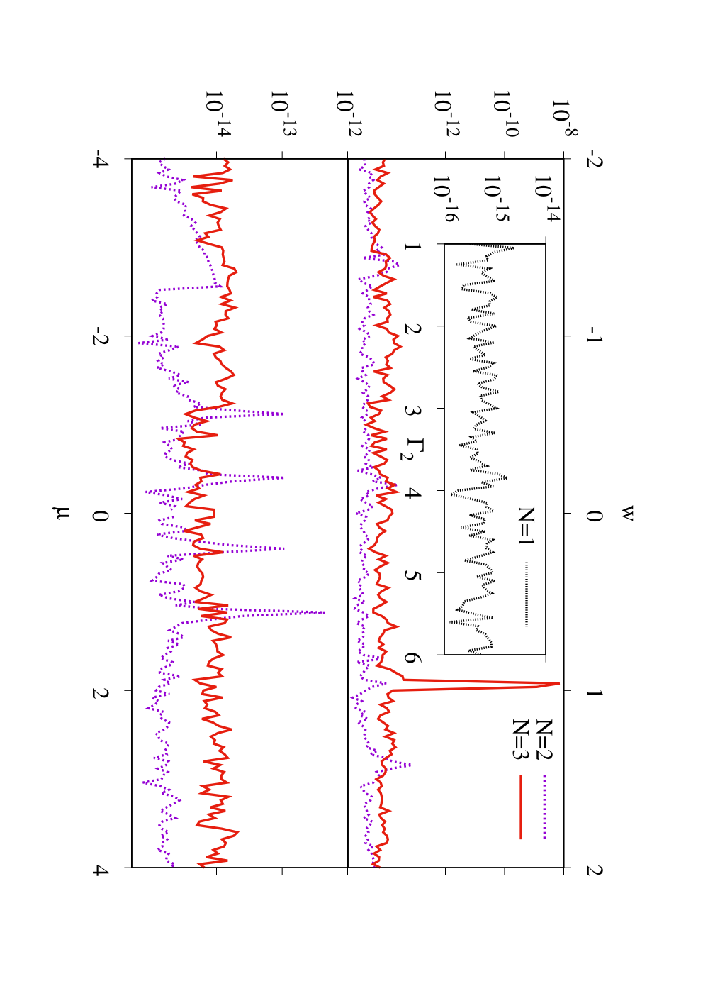
In order to check the reliability of the proposal, the state obtained by the procedure recounted above has been compared against results extracted by other methods in a number of accessible instances. For the case analytical results can be derived considering the following baths operators
| (96) | |||
| (97) |
In this particular case the constants and simply do not show up in the Hamiltonian. Replacing (19) in (21) and solving yield
| (98) |
In order to assess the difference against the state calculated by the folding procedure, , the following error estimate is introduced
| (99) |
where . The inset in figure 1 shows as a function of keeping constant.
In order to test chains with and a couple of baths are added on both ends in the following fashion
| (100) | |||
| (101) |
Since in this instance there is no analytical solution, the NESS is calculated numerically as the eigenstate of (19) associated with zero eigenvalue. Comparative errors can be seen in figure 1. As can be observed, the protocol delivers the correct state for even- as well as odd- up to roundoff errors, which for the cases and might even come from the benchmark calculation. Lack of analytical results for arbitrary makes it difficult to analyze error scaling, but the study of a similar method on the Kitaev chain reported in reslen5 indicates that relative errors saturate for chains of some tens of sites to the order of magnitude of the square root of machine precision.
V Results

In solid state systems Majorana fermions are seen as collective excitations rather than actual particles. Because the formalism assigns two Majoranas to every single body state, it is common for Majorana fermions to couple with their twin mode, giving in this way rise to localized excitations. However, it is possible that some Majorana fermions did not pair, bringing about interesting phases that are highly non-local and robust, also characterized as topological. The Kitaev chain is a particular scenario where this behavior can be studied in detail due to the model integrability. Such a possibility is however no longer an option in systems lacking some level of analyticity. As an alternative, reference reslen5 introduces an operational criterion that allows to determine whether the state contains uncoupled Majorana fermions localized on the edges. The witness quantity is the thermodynamic limit of the End-to-End Correlations (EEC) defined as
| (102) |
The equivalent in the second space of the expression in brackets can be worked out as follows
| (103) |
Correlations can therefore be calculated as
| (104) |
The value of can be estimated analyzing the behavior of EEC against growing . However, given the difficulties in fitting some sets of data, in this work the analysis is limited to determining whether or not vanishes. Another observable of interest is the actual mean number of particles at a given position, which comes from
| (105) |
Numerical simulations were carried out in Kitaev chains subject to baths described by (100) and (101). The study has been limited to baths with a particle-injection effect since this seems to be the most convenient scenario to enhance EEC. Bath constants are therefore set to and . The size of the tensorial representation is a dynamical variable an depends on the requirements of each particular computation. This explains why the parameter known as is not reported. When is fixed there is a limit on the number of basis states available to the system, and although this allows to obtain results for large chains, it also affects the accuracy of the simulation, especially when long range correlations are strong.
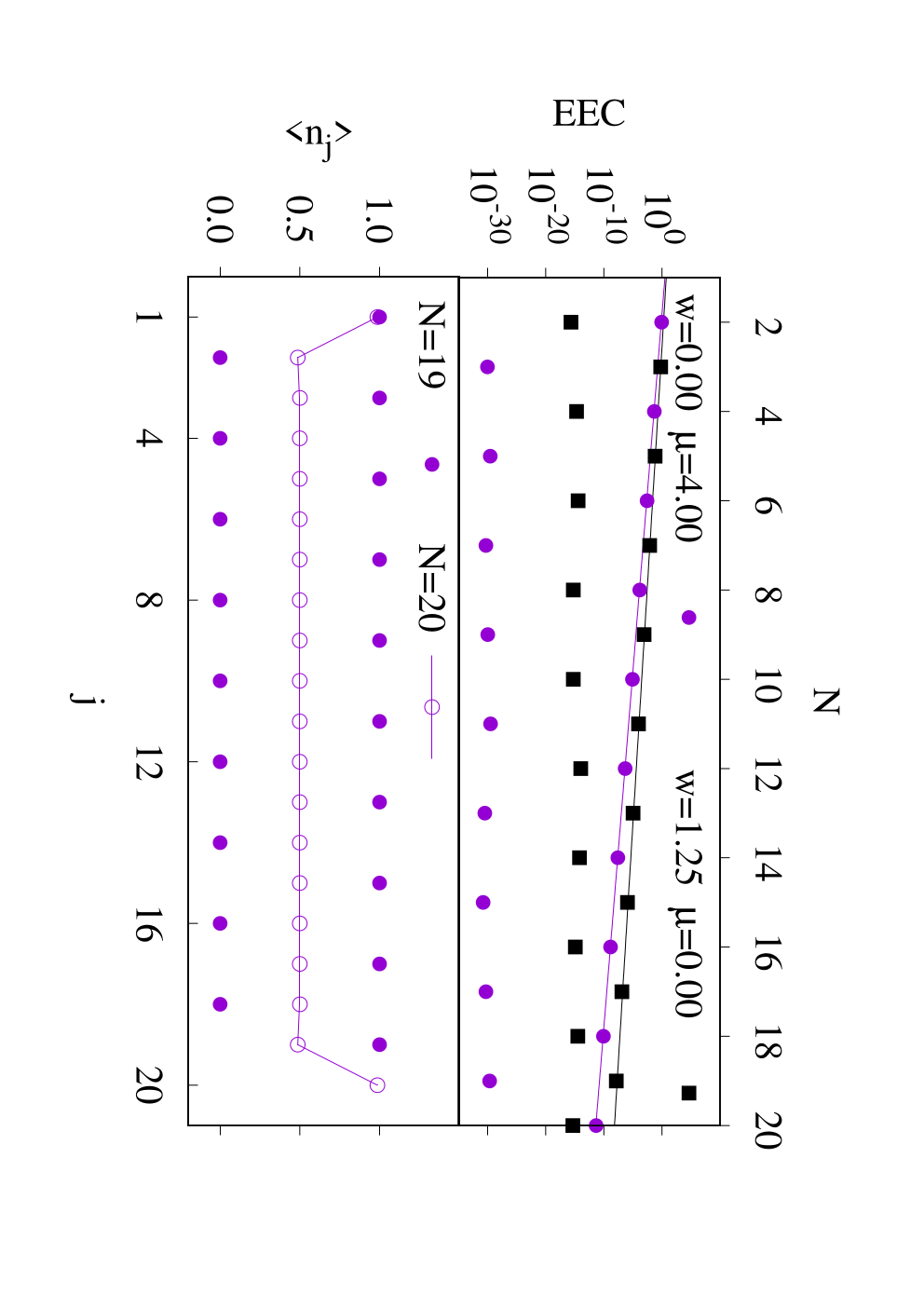
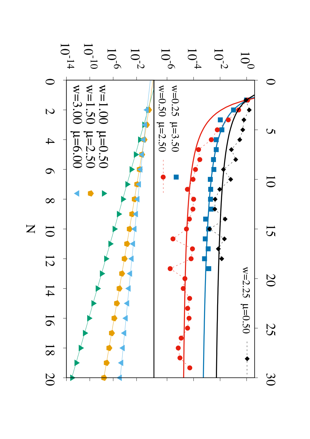
Let us initially address the results depicted in figure 2. It might appear atypical that EEC can be nonzero in chains with zero hopping. On closer inspection it is seen that chains of odd size display a separable particle distribution with zero correlations, but in chains of even size an unstowed particle spreads all over the chain interior and so enhances EEC. However, this correlations decay exponentially with the chain size and make no contribution to . This latter fact is characteristic of other configurations, for instance when , although the finite-size mechanism is different since in such a case hopping is nonzero. Scanning over a grid of parameters it is possible to identify cases where, in contrast, correlations seem to tend toward finite values, as shown in figure 3. A trait that make it difficult to estimate quantitatively is that finite-size effects are strong and fitting attempts proved inconclusive. Additionally, if finite-size effects are being enhanced by boundary effects, the zig-zag pattern observed in the top pannel of figure 3 might go on nonstop, specifically in chains with long range correlations. Regardless, the observed dependency shows a pattern that is different from exponential decay. Having established these two profiles, a potential phase diagram has been put together in figure 4. The signs of or do not affect correlations so that the diagram has been synthesized in a single quadrant. An useful benchmark is the bathless chain, which is known to display uncoupled Majoranas in the region . In this respect there seems to be coincidence for values of greater than , discounting the line . Apart from that, exponential decay is seen along the whole line , while convergence around finite values can be seen in sectors where equilibrium states do not display uncoupled Majoranas, like close to the axis. The opposite behavior, i.e., exponential decay in sectors where the chain in equilibrium displays uncoupled Majoranas, takes place over the axis and in some points close to the equilibrium boundary and the line . In general terms it can be said that the system has in some degree resisted the detrimental effects of the baths on its long range excitations, even has gained in some sectors of the phase diagram, although the intensity of these excitations has been negatively affected with respect to the equilibrium case. Simulation times are typically longer for chains with stronger EEC, but long times can be displayed by chains with vanishing as well, specifically along the lines , and , as can be seen in the scaling profiles of figure 5. Such scaling profiles reveal a gain in simulation efficiency for all sets of parameters, even for those with exponential growth, because the problem dimension scales exponentially with a slope that is no less than .

VI Conclusions
A method to compute the NESS of a general quadratic Fermi Hamiltonian under the action of linear baths has been introduced and tested in a system known as the Kitaev chain where a topological phase bearing uncoupled Majorana Fermions is well characterized under equilibrium conditions. The protocol has been used to study the incidence of uncoupled Majorana fermions in chains subject to baths at the ends using the limit of correlations as a measure. The case in favor of uncoupled Majoranas in some regions of parameter space is supported by the converging trends of graphics of correlations vs. chain size. A tentative phase diagram has been presented and contrasted with the equilibrium analogue showing more coincidence for large values of the hopping constant. Simulation times display potential scaling against chain size for most sets of parameters, thus evidencing an improved performance with respect to the scaling of the dimension of the original physical space.
The protocol introduced in this study has direct applications in a wide variety of physical configurations of relevance. The second space approach of section II is known as a super-fermion representation in the context of electron transport kosov and it is apparent that the methods introduced here suit this field. Changes can be incorporated to adjust the protocol in the direction of the dependence of state with time. From this the net current flux between the chain and the exterior could be calculated as the numerical derivative of the total number of particles in the chain with respect to time. Another way of studying transport phenomena is to add a tilted potential through a dependency of with respect to position in (1) and then consider the current through the chain as proportional to the mean value of the momentum operator. When the fermion modes are sufficiently-localized Wannier-functions, such an operator becomes a sum of next-neighbor hopping terms. Voltage would correspond to the slope of the tilted potential. In the same spirit, disorder effects can be studied by assigning random coefficients to the chemical potential across the chain. None of the aforementioned proposals would require any structural change in the method that has been presented, which can be used as long as the Hamiltonian be quadratic in the fermionic modes, and the bath terms be linear. The effect of lead contacts and the calculation of zero-bias conductance could be addressed following the proposal in reference Doornenbal, which involves simulating the contacts as a set of momentum modes coupled to the chain ends. Interaction with light can be studied semiclasically without major changes to the current formulation. Spin systems can be addressed via a Jordan-Wigner transformation. A more challenging project is to develop an analogous formalism that worked with interacting systems. This is because in such a case it is not clear how to write the state as a product of sums of operators. An option is to utilize expression (95) as an ansatz. Another option is to try to model interaction in a mean-field fashion. Also relevant is the question of what are the minimum conditions a transfer matrix must fulfill so that it can be folded in an applicable way. Similarly, the method looks suitable to study quantities that involve the whole density matrix, as for example mixedness or entropy, since the state is obtained in full. Also of interest are the insight possibilities that the method can offer to the field of fermionic systems. In equation (95) a fermion density-matrix is written as a series of unitary operations. What this decomposition can provide in terms of characterization of the physical state remains to be explored. Thus far evidence suggests that traces of uncoupled Majorana fermions and long range correlations can be identified for specific sets of parameters in Kitaev chains exposed to baths on the ends that break the mechanism of topological protection. Moreover, the notion of folding of modes can be used to study open quantum systems.
Financial support by Vicerrectoría de Investigaciones, Extensión y Proyección Social from Universidad del Atlántico is gratefully acknowledged.
References
- (1) A. Kitaev Unpaired majorana fermions in quantum wires Physics-Uspekhi 44 131, (2001).
- (2) R. Aguado Majorana quasiparticles in condensed matter La Rivista del Nuovo Cimento 11 523 (2017).
- (3) R. Lutchyn, E. Bakkers, L. Kouwenhoven, P. Krogstrup, C. Marcus and Y. Oreg Majorana zero modes in superconductor-semiconductor heterostructures Nature Reviews Materials 3 52 (2018).
- (4) A. Carmele, M. Heyk, C. Kraus and M. Dalmonte Streched exponential decay of Majorana edge modes in many-body localized Kitaev chains under dissipation Physical Review B 92 195107 (2015).
- (5) T. Prosen and B. Zunkovi Exact solution of Markovian master equations for quadratic Fermi systems: thermal baths, open XY spin chains and non-equilibrium phase transition New Journal of Physics 12 025016 (2010).
- (6) T. Prosen and I. Pizorn Quantum Phase Transition in a Far-from-Equilibrium Steady State of an XY Spin Chain Physical Review Letters 101 105701 (2008).
- (7) T. Prosen and M. Znidaric Long-range order in nonequilibrium interacting quantum spin chains Physical Review Letters 105 060603 (2010).
- (8) T. Prosen Exact Nonequilibrium Steady State of a Strongly Driven Open XXZ Chain Physical Review Letters 107 137201 (2011).
- (9) P. Kos and T. Prosen Time-dependent correlation functions in open quadratic fermionic systems Journal of Statistical Mechanics: Theory and Experiment 123103 (2017).
- (10) J. Reslen End-to-end correlations in the Kitaev chain Journal of Physics Communications 2 105006 (2018).
- (11) G. Lindblad On the generators of quantum dynamical semigroups Communications in Mathematical Physics 48 119, (1976).
- (12) S. Bravyi and R. Konig Classical simulation of dissipative fermionic linear optics Quantum Information and Computation 12 0924 (2012).
- (13) T. Prosen Third quantization: a general method to solve master equations for quadratic open Fermi systems New Journal of Physics 10 043026 (2008).
- (14) M. Schmutz Real-time Green’s functions in many body problems Zeitschrift fur Physik B 30 97 (1978).
- (15) F. Schwabl Advanced quantum mechanics, 4th edition (Springer, Berlin, 2008).
- (16) T. Prosen Matrix product solutions of boundary driven quantum chains Journal of Physics A: Mathematical and Theoretical 48 373001 (2015).
- (17) R. Orus A practical introduction to tensor networks: Matrix product states and projected entangled pair states Annals of Physics 349 117 (2014).
- (18) A. Dzhioev and D. Kosov Super-fermion representation of quantum kinetic equations for the electron transport problem The Journal of Chemical Physics 134 044121 (2011).
- (19) R. Doornenbal, G. Skantzaris and H. Stoof Conductance of a finite Kitaev chain Physical Review B 91 045419 (2015).
Appendix A Liouvillian coefficients in the second representation
Replacing the Majorana operators defined in equation (22) and expanding, Liouvillian (19) becomes
| (106) |
Although in this expression the Liouvillian coefficients do not form an antisymmetric matrix, the anticommutation properties of Majorana fermions let us define conforming coefficients as follows
| (107) |