G-Learner and GIRL:
Goal Based Wealth Management with Reinforcement LearningThanks: Igor Halperin is a Research Professor in Financial Engineering at NYU, and an AI Research associate at Fidelity Investments. E-mail: ighalp@gmail.com. The views presented in this paper are of the author, and do not necessarily represent the views of his employer. The standard disclaimer applies. The author thanks Lisa Huang for helpful discussions.
Abstract
We present a reinforcement learning approach to goal based wealth management problems such as optimization of retirement plans or target dated funds. In such problems, an investor seeks to achieve a financial goal by making periodic investments in the portfolio while being employed, and periodically draws from the account when in retirement, in addition to the ability to re-balance the portfolio by selling and buying different assets (e.g. stocks). Instead of relying on a utility of consumption, we present G-Learner: a reinforcement learning algorithm that operates with explicitly defined one-step rewards, does not assume a data generation process, and is suitable for noisy data. Our approach is based on G-learning (Fox et al. 2015) — a probabilistic extension of the Q-learning method of reinforcement learning. In this paper, we demonstrate how G-learning, when applied to a quadratic reward and Gaussian reference policy, gives an entropy-regulated Linear Quadratic Regulator (LQR). This critical insight provides a novel and computationally tractable tool for wealth management tasks which scales to high dimensional portfolios. In addition to the solution of the direct problem of G-learning, we also present a new algorithm, GIRL, that extends our goal-based G-learning approach to the setting of Inverse Reinforcement Learning (IRL) where rewards collected by the agent are not observed, and should instead be inferred. We demonstrate that GIRL can successfully learn the reward parameters of a G-Learner agent and thus imitate its behavior. Finally, we discuss potential applications of the G-Learner and GIRL algorithms for wealth management and robo-advising.
.
1 Introduction
Mean-variance Markowitz optimization (MVO) (Markowitz 1959) remains one of the most commonly used tools in wealth management. Portfolio objectives in this approach are defined in terms of expected returns and covariances of assets in the portfolio, which may not be the most natural formulation for retail investors. Indeed, the latter typically seek specific financial goals for their portfolios. For example, a contributor to a retirement plan may demand that the value of their portfolio at the age of his or her retirement be at least equal to, or preferably larger than, some target value .
Goal-based wealth management offers some valuable perspectives into optimal structuring of wealth management plans such as retirement plans or target date funds. The motivation for operating in terms of wealth goals can be more intuitive (while still tractable) than the classical formulation in terms of expected excess returns and variances. To see this, let be the final wealth in the portfolio, and be a certain target wealth level at the horizon . The goal-based wealth management approach of Browne 1996 and Das et al. 2018 uses the probability of final wealth to be above the target level as an objective for maximization by an active portfolio management. This probability is the same as the price of a binary option on the terminal wealth with strike : . Instead of a utility of wealth such as e.g. a power or logarithmic utility, this approach uses the price of this binary option as the objective function. This idea can also be modified by using a call option-like expectation , instead of a binary option. Such an expectation quantifies how much the terminal wealth is expected to exceed the target, rather than simply providing the probability of such event11 1 The problem of optimal consumption with an investment portfolio is frequently referred to as the Merton consumption problem, after the celebrated work of Robert Merton who formulated this problem as a continuous-time optimal control problem with log-normal dynamics for asset prices (Merton 1971). As optimization in problems involving cash injections instead of cash withdrawals formally corresponds to a sign change of one-step consumption in the Merton formulation, we can collectively refer to all types of wealth management problems involving injections or withdrawals of funds at intermediate time steps as a generalized Merton consumption problem. .
This treatment of the goal-based utility function can be implemented in a reinforcement learning (RL) framework for discrete-time planning problems. In contrast to the Merton consumption approach, RL does not require specific functional forms of the utility nor does it require that the dynamics of the assets be treated as log-normal. Thus in theory, RL can be viewed as a data-driven extension of dynamic programming (Sutton and Barto 2018). In practice, a substantial challenge with the RL framework is the curse of dimensionality — portfolio allocation as a continuous action space Markov Decision Process (MDP) requires techniques such as deep Q-learning or other function approximation methods combined e.g. with the Least Squares Policy Iteration (LSPI) method (Lagoudakis and Parr 2003). The latter has exponential complexity with increasing stocks in the portfolio, and the former is cumbersome, highly data intensive, and heavily relies on heuristics for operational efficiency. For more details, see e.g. (Dixon et al. 2020).
In this paper, we present G-learning (Fox et al. 2015) — a probabilistic extension of Q-learning which scales to high dimensional portfolios while providing a flexible choice of utility functions. To demonstrate the utility of G-learning, we consider a general class of wealth management problems: optimization of a defined contribution retirement plan, where cash is injected (rather than withdrawn) at each time step. In contrast to methods based on a utility of consumption, we adopt a more “RL-native” approach by directly specifying one-step rewards. Such an approach is sufficiently general to capture other possible settings, such as e.g. a retirement plan in a decumulation (post-retirement) phase, or target based wealth management. Previously, G-learning was applied to dynamic portfolio optimization in (Halperin and Feldshteyn 2018), while here we extend this approach to portfolio management involving cashflows at intermediate time steps.
A key step in our formulation is that we define actions as absolute (dollar-valued) changes of asset positions, instead of defining them in fractional terms, as in the Merton approach (Merton 1971). This enables a simple transformation of the optimization problem into an unconstrained optimization problem, and provides a semi-analytical solution for a particular choice of the reward function. As will be shown below, this approach offers a tractable setting for both the direct reinforcement learning problem of learning the optimal policy which maximizes the total reward, and its inverse problem where we observe actions of a financial agent but not the rewards received by the agent. Inference of the reward function from observations of states and actions of the agent is the objective of Inverse Reinforcement Learning (IRL). After we present G-Learner — a G-learning algorithm for the direct RL problem, we will introduce GIRL (G-learning IRL) — a framework for inference of rewards of financial agents that are “implied” by their observed behavior. The two practical algorithms, G-Learner and GIRL, can be used either separately or in a combination, and we will discuss their potential joint applications for wealth management and robo-advising.
The paper is organized as follows. In Section 2, we introduce G-learning and explain how it generalizes the more well known Q-learning method for reinforcement learning. Section 3 introduces the problem of portfolio optimization for a defined contribution retirement plan. Then in Section 4, we present the G-Learner: a G-learning algorithm for portfolio optimization with cash injection and consumption. The GIRL algorithm for performing IRL of financial agents is introduced in Section 5. Section 6 presents the results of our implementation and demonstrates the ability of G-learner to scale to high dimensional portfolio optimization problems, and the ability of GIRL to make inference of the reward function of a G-Learner agent. Section 7 concludes with ideas for future developments in G-learning for wealth management and robo-advising.
2 G-learning
In this section, we provide a short but self-contained overview of G-learning as a probabilistic extension of the popular Q-learning method in reinforcement learning. We assume some familiarity with constructs in dynamic programming and reinforcement learning, see e.g. (Sutton and Barto 2018), or (Dixon et al. 2020) for a more finance-focused introduction. In particular, we assume that the reader is familiar with the notions of value function, action-value function, and the Bellman optimality equations. Familiarity with Q-learning is desirable but not critical for understanding this section, however for the benefit of the informed reader, a short informal summary of the differences is as follows:
- •
Q-learning is an off-policy RL method with a deterministic policy.
- •
G-Learning is an off-policy RL method with a stochastic policy. G-learning can be considered as an entropy-regularized Q-learning, which may be suitable when working with noisy data. Because G-learning operates with stochastic policies, it amounts to a generative RL model.
2.1 Bellman optimality equation
More formally, let be a state vector for an agent that summarizes the knowledge of the environment that the agent needs in order to perform an action at time step 22 2 Here we assume a discrete-time setting where time is measured in terms of integer-valued number of elementary time steps .. Let be a random reward collected by the agent for taking action at time when the state of the environment is . Assume that all future actions for future time steps are determined according to a policy which specifies which action to take when the environment is in state . We note that policy can be deterministic as in Q-learning, or stochastic as in G-learning, as we will discuss below.
For a given policy , the expected value of cumulative reward with a discount factor , conditioned on the current state , defines the value function
| (1) |
Here stands for the expectation of future states and actions, conditioned on the current state and policy .
Let be the optimal policy, i.e. the policy that maximizes the total reward. This policy corresponds to the optimal value function, denoted . The latter satisfies the Bellman optimality equation (see e.g. (Sutton and Barto 2018))
| (2) |
Here stands for an expectation conditional on the current state and action . The optimal policy can be obtained from as follows:
| (3) |
The goal of Reinforcement Learning (RL) is to solve the Bellman optimality equation based on samples of data. Assuming that an optimal value function is found by means of RL, solving for the optimal policy takes another optimization problem as formulated in Eq.(3).
2.2 Entropy-regularized Bellman optimality equation
Let us begin by reformulating the Bellman optimality equation using a Fenchel-type representation:
| (4) |
Here denotes a set of all valid distributions. Eq.(4) is equivalent to the original Bellman optimality equation (2), because for any , we have . Note that while we use discrete notations for simplicity of presentation, all formulae below can be equivalently expressed in continuous notations by replacing sums by integrals. For brevity, we will denote the expectation as in what follows.
The one-step information cost of a learned policy relative to a reference policy is defined as follows (Fox et al. 2015):
| (5) |
Its expectation with respect to the policy is the Kullback-Leibler (KL) divergence of and :
| (6) |
The total discounted information cost for a trajectory is defined as follows:
| (7) |
The free energy function is defined as the value function (4) augmented by the information cost penalty (7) which is added using a regularization parameter :
| (8) |
The free energy, , is the entropy-regularized value function, where the amount of regularization can be tuned to the level of noise in the data. The regularization parameter in Eq.(8) controls a trade-off between reward optimization and proximity of the optimal policy to the reference policy, and is often referred to as the “inverse temperature” parameter, using the analogy between Eq.(8) and free energy in physics, see e.g. (Dixon et al. 2020). The reference policy, , provides a “guiding hand” in the stochastic policy optimization process that we now describe.
A Bellman equation for the free energy function is obtained from Eq.(8):
| (9) |
For a finite-horizon setting with a terminal reward , Eq.(9) should be supplemented by a terminal condition
| (10) |
where the final action maximizes the terminal reward for the given terminal state . Eq.(9) can be viewed as a soft probabilistic relaxation of the Bellman equation for the value function, with the KL information cost penalty (5) as a regularization controlled by the inverse temperature . In addition to such a regularized value function (free energy), we will next introduce an entropy regularized Q-function.
2.3 G-function: an entropy-regularized Q-function
Similar to the action-value function, we define the state-action free energy function as (Fox et al. 2015)
| (11) | |||||
where in the last equation we used the fact that the first action in the G-function is fixed, and hence when we condition on .
If we now compare this expression with Eq.(8), we obtain the relation between the G-function and the free energy :
| (12) |
This functional is maximized by the following distribution :
| (13) | |||
The free energy (12) evaluated at the optimal solution (13) becomes
| (14) |
Using Eq.(14), the optimal action policy can be written as follows :
| (15) |
Eqs.(14), (15), along with the first form of Eq.(11) repeated here for convenience:
| (16) |
constitute a system of equations for G-learning (Fox et al. 2015) that should be solved self-consistently for , and by backward recursion for , with terminal conditions
| (17) | |||
We will next show how G-learning can be implemented in the context of (direct) reinforcement learning.
2.4 G-learning
In the RL setting when rewards are observed, the system Eqs.(14, 15, 16) can be reduced to one non-linear equation. Substituting the augmented free energy (14) into Eq.(16), we obtain
| (18) |
This equation provides a soft relaxation of the Bellman optimality equation for the action-value Q-function, with the G-function defined in Eq.(11) being an entropy-regularized Q-function (Fox et al. 2015). The ”inverse-temperature” parameter in Eq.(18) determines the strength of entropy regularization. In particular, if we take a “zero-temperature” limit , we recover the original Bellman optimality equation for the Q-function. Because the last term in (18) approximates the function when is large but finite, for a particular choice of a uniform reference distribution , Eq.(18) is known in the literature as “soft Q-learning”.
For finite values , in a setting of Reinforcement Learning with observed rewards, Eq.(18) can be used to specify G-learning (Fox et al. 2015): an off-policy time-difference (TD) algorithm that generalizes Q-learning to noisy environments where an entropy-based regularization is appropriate.
The G-learning algorithm of Fox et al. 2015 was specified in a tabulated setting where both the state and action space are finite. In our case, we model MDPs in high-dimensional continuous state and action spaces. Respectively, we cannot rely on a tabulated G-learning, and need to specify a functional form of the action-value function, or use a non-parametric function approximation such as a neural network to represent its values. An additional challenge is to compute a multidimensional integral (or a sum) over all next-step actions in Eq.(18). Unless a tractable parameterization is used for and , repeated numerical integration of this integral can substantially slow down the learning.
To summarize, G-learning is an off-policy, generative reinforcement learning algorithm with a stochastic policy. In contrast to Q-learning, which produces deterministic policies, G-learning generally produces stochastic policies, while the deterministic Q-learning policies are recovered in a zero-temperature limit . In the next section, we will build an approach to goal-based wealth management based on G-learning. Later in this paper, we will also consider applications of G-learning for Inverse Reinforcement Learning (IRL).
3 Portfolio optimization for a defined contribution retirement plan
Let us begin by considering a simplified model for retirement planning. We assume a discrete-time process with steps, so that is the (integer-valued) time horizon. The investor/planner keeps the wealth in assets, with being the vector of dollar values of positions in different assets at time , and being the vector of changes in these positions. We assume that the first asset with is a risk-free bond, and other assets are risky, with uncertain returns whose expected values are . The covariance matrix of return is of size .
Optimization of a retirement plan involves optimization of both regular contributions to the plan and asset allocations. Let be a cash installment in the plan at time . The pair can thus be considered the action variables in a dynamic optimization problem corresponding to the retirement plan.
We assume that at each time step , there is a pre-specified target value of a portfolio at time . We assume that the target value at step exceeds the next-step value of the portfolio, and we seek to impose a penalty for under-performance relative to this target. To this end, we can consider the following expected reward for time step :
| (19) |
Here the first term is due to an installment of amount at the beginning of time period , the second term is the expected negative reward from the end of the period for under-performance relative to the target, and the third term approximates transaction costs by a convex functional with the parameter matrix , and serves as a regularization.
The one-step reward (19) is inconvenient to work with due to the rectified non-linearity under the expectation. Another problem is that decision variables and are not independent but rather satisfy the following constraint
| (20) |
which simply means that at every time step, the total change in all positions should equal the cash installment at this time.
We therefore modify the one-step reward (19) in two ways: we replace the first term using Eq.(20), and approximate the rectified non-linearity by a quadratic function. The new one-step reward is
| (21) |
The new reward function (21) is attractive on two counts. First, it explicitly resolves the constraint (20) between the cash injection and portfolio allocation decisions, and thus converts the initial constrained optimization problem into an unconstrained one. We remind the reader that this differs from the Merton model where allocation variables are defined as fractions of the total wealth, and thus are constrained by construction. The approach based on dollar-measured actions both reduces the dimensionality of the optimization problem, and makes it unconstrained. When the unconstrained optimization problem is solved, the optimal contribution at time can be obtained from Eq.(20).
The second attractive feature of the reward (21) is that it is quadratic in actions , and is therefore highly tractable. On the other hand, the well known disadvantage of quadratic rewards (penalties) is that they are symmetric, and penalize both scenarios and , while in fact we only want to penalize the second class of scenarios. To mitigate this drawback, we can consider target values that are considerably higher than the time- expectation of the next-period portfolio value. For example, one simple choice could be to set the target portfolio as a linear combination of a portfolio-independent benchmark and the current portfolio growing with a fixed rate :
| (22) |
where is a relative weight of the portfolio-independent and portfolio-dependent terms, and is a parameter that defines the desired growth rate of the current portfolio whose value is . For a sufficiently large values of and , such a target portfolio would be well above the current portfolio at all times, and thus would serve as a reasonable proxy to the asymmetric measure (19). The advantage of such a parameterization of the target portfolio is that both the “desired growth” parameter and the mixture parameter can be learned from an observed behavior of a financial agent in the setting of Inverse Reinforcement Learning (IRL), as we will discuss in Sec. 5. In what follows, we use Eq.(22) as our specification of the target portfolio.
We note that a quadratic loss specification relative to a target time-dependent wealth level is a popular choice in the recent literature on wealth management. One example is provided by Lin et al. 2019 who develop a dynamic optimization approach with a similar squared loss function for a defined contribution retirement plan. A similar approach which relies on a direct specification of a reward based on a target portfolio level is known as “goal-based wealth management” (Browne 1996; Das et al. 2018).
The square loss reward specification is very convenient, as it allows one to construct optimal policies semi-analytically. Here we will demonstrate how to build a semi-analytical scheme for computing optimal stochastic consumption-investment policies for a retirement plan — the method is sufficiently general for either a cumulation or de-cumulation phase. For other specifications of rewards, numerical optimization and function approximations (e.g. neural networks) would be required.
The expected reward (21) can be written in a more explicit quadratic form if we denote asset returns as where the first component is the risk-free rate (as the first asset is risk-free), and ) where is an idiosyncratic noise with covariance of size . Substituting this expression in Eq.(21), we obtain
where
| (26) | |||
Assuming that the expected returns , covariance matrix and the benchmark are fixed, the vector of free parameters defining the reward function is thus .
4 G-learner for retirement plan optimization
To solve the optimization problem, we use a semi-analytical formulation of G-learning with Gaussian time-varying policies (GTVP). In what follows, we will refer to our specific algorithm implementing G-learning with our model specifications as the G-Learner algorithm, to differentiate our model from more general models that could potentially be constructed using G-learning as a general RL method.
We start by specifying a functional form of the value function as a quadratic form of :
| (27) |
where are parameters that can depend on time via their dependence on the target values and the expected returns . The dynamic equation takes the form:
| (28) |
Note that the only features used here are the expected asset returns for the current period . We assume that the expected asset returns are available as an output of a separate statistical model using e.g. a factor model framework. The present formalism is agnostic to the choice of the expected return model.
Coefficients of the value function (27) are computed backward in time starting from the last maturity . For , the quadratic reward (3) can be optimized analytically by the following action:
| (29) |
where we defined as follows
| (30) |
Note that the optimal action is a linear function of the state. Another interesting point to note is that the last term that describes convex transaction costs in Eq.(3) produces regularization of matrix inversion in Eq.(29).
As for the last time step we have , coefficients can be computed by plugging Eq.(29) back in Eq.(3), and comparing the result with Eq.(27) with . This provides terminal conditions for parameters in Eq.(27):
| (31) | |||||
For an arbitrary time step , we use Eq.(28) to compute the conditional expectation of the next-period F-function in the Bellman equation as follows:
where , and similarly for and . This is a quadratic function of and , and has the same structure as the quadratic reward in Eq.(3). Plugging both expressions in the Bellman equation
we see that the action-value function should also be a quadratic function of and :
| (35) |
where
| (36) | |||
After the action-valued function is computed as per Eqs.(4), what remains is to compute the F-function for the current step:
| (37) |
A reference policy is Gaussian:
| (38) |
where the mean value is a linear function of the state :
| (39) |
Integration over in Eq.(37) is performed analytically using the well known -dimensional Gaussian integration formula
| (40) |
where denotes the determinant of matrix .
Note that, unlike in the Merton approach (Merton 1971) or in traditional Markowitz portfolio optimization (Markowitz 1959), here we work with unconstrained variables that do not have to sum up to one, and therefore an unconstrained multivariate Gaussian integration readily applies here. Remarkably, this implies that once the decision variables are chosen appropriately, portfolio optimization for wealth management tasks may in a sense be an easier problem than portfolio optimization that does not involve intermediate cashflows, and is often formulated using self-financing conditions.
Performing the Gaussian integration and comparing the resulting expression with Eq.(27), we obtain for its coefficients:
| (41) | |||||
where we use the auxiliary parameters
| (42) | |||||
The optimal policy for the given step is given by
| (43) |
Using here the quadratic action-value function (35) produces a new Gaussian policy :
| (44) |
where
| (45) | |||||
Therefore, policy optimization for G-learning with quadratic rewards and Gaussian reference policy amounts to the Bayesian update of the prior distribution (38) with parameters updates to the new values defined in Eqs.(4). These quantities depend on time via their dependence on the targets and expected asset returns .
For a given time step , the G-learning algorithm keeps iterating between the policy optimization step that updates policy parameters according to Eq.(4) for fixed coefficients of the - and -functions, and the policy evaluation step that involves Eqs.(35, 4, 4) and solves for parameters of the - and -functions given policy parameters. Note that convergence of iterations for is guaranteed as . At convergence of iteration for time step , Eqs.(35, 4, 4) and (44) together solve one step of G-learning. The calculation then proceeds by moving to the previous step , and repeating the calculation, all the way back to the present time.
The additional step needed from G-learning for the present problem is to find the optimal cash contribution for each time step by using the budget constraint (20). As G-learning produces Gaussian random actions , Eq.(20) implies that the time- optimal contribution is Gaussian distributed with mean . The expected optimal contribution thus has a part that is independent of the portfolio value, and a part that depends on the current portfolio. This is similar e.g. to a linear specification of the defined contribution with a deterministic policy in Lin et al. 2019.
It should be noted that in practice, we may want to impose constraints on cash installments . For example, we could impose band constraints with some upper bound . Such constraints can be easily added to the framework. To this end, we need to replace the exactly solvable unconstrained least squares problem with a constrained least squares problem. This can be done without a substantial increase of computational time using efficient off-the-shell convex optimization software. Note that enforcing constraints on the resulting cash-flows in our approach amounts to optimization with one constraint, instead of two constraints as in the Merton approach.
5 GIRL: G-learning IRL
So far in this paper, we considered the setting of (direct) reinforcement learning, when the agent (investor) learns while observing the rewards, and optimizes the policy so that the expected cumulative reward (regularized by the KL information cost) is maximized. This setting is suitable when the investor explicitly defines his or her reward function.
In many cases of practical interest, an individual investor may not be able to explain his or her utility function used for trading decision-making, which can instead be rule-driven (or driven by other model not formulated in RL terms). Alternatively, when an agent (investor) is a subject of behavioral inference to a different agent (a researcher or robo-advisor), the latter has access to observed trajectories (states and actions) of the agent, but not to rewards received by the agent. Such cases where rewards are not available belong in the realms of Inverse Reinforcement Learning (IRL) whose objective is to recover both the reward function of the agent and the optimal policy, see e.g. (Dixon et al. 2020) for a review.
In this section, we consider the IRL problem with G-learning, and present an algorithm we call GIRL (G-learning IRL) whose objective is to make inference of the reward function of an individual agent such as a retirement plan contributor or an individual brokerage account holder. That is, we assume that we are given a history of dollar-nominated asset positions in an investment portfolio, jointly with an agent’s decisions that include both injections or withdrawals of cash from the portfolio and asset allocation decisions. Additionally, we are given historical values of asset prices and expected asset returns for all assets in the investor universe. As previously in the paper, we can consider a portfolio of stocks and a single bond, but the same formalism can be applied to other types of assets.
Assume that we have historical data that includes a set of trajectories where of state-action pairs where trajectory starts at some time and runs until time . Consider a single trajectory from this collection, and set for this trajectory the start time and the end time . As individual trajectories are considered independent, they will enter additively in the final log-likelihood of the problem. We assume that dynamics are Markovian in the pair , with a generative model where stands for a vector of model parameters, and is the action policy given by Eq.(43).
The probability of observing trajectory is given by the following expression
| (46) |
Here is a marginal probability of at the start of the -th demonstration. Assuming that the initial values are fixed, this gives the following log-likelihood for data observed for trajectory :
| (47) |
Transition probabilities entering this expression can be obtained from the state equation
| (48) |
where is a Gaussian noise with covariance (see Eq.(28)). Writing where is the value of a bond position and are the values of positions in risky assets, and similarly for and , this produces transition probabilities
| (49) |
where the factor captures the deterministic dynamics of the bond part of the portfolio. As this term does not depend on model parameters, we can drop it from the log-transition probability, along with a constant term . This produces
| (50) |
Substituting Eqs.(43), (35), (50) into the trajectory log-likelihood (47), we put it in the following form:
| (51) |
where and are defined by Eqs.(35) and (27). The log-likelihood (51) is a function of model parameter vector (recall that is a regularization hyper-parameter which should not be optimized in-sample). We can simplify the problem by setting and (i.e. take a constant mean in the prior). In this case, the vector of model parameter to learn with IRL inference is . A “proper” IRL setting would correspond to only learning parameters of the reward function while keeping parameters fixed (i.e. estimated outside of the IRL model). Optimization can be performed using available off-the-shelf software. In our implementation, we use the Adam optimization method within PyTorch to optimize the negative log-likelihood function.
6 Numerical examples
To illustrate the G-learner and GIRL algorithms for goal based wealth management, we use a simple simulated environment that mimics the working of equity return models (sometimes referred to as “alpha-models”) which are expected in practice to be weak predictors of realised returns. The advantage of such a simulated environment is that it allows us to define the “ground truth” and thus demonstrate the performance of both algorithms. We remind the reader that while we use simulated data to show the performance of our algorithms, the latter are model free as they are independent of a model of stock-price dynamics.
The investment horizon is set to 7.5 years and the portfolio rebalancing and consumption occur quarterly (over 30 periods). In this simplified setting, the portfolio is assumed to be initially equally weighted, with $1000 allocated equally between stocks and a risk free bond. We assume a fixed risk free annual rate, , stock transactions costs are 1.5% of the stock price and risk-free bond transactions costs are 5%. The benchmark portfolio is initially set equal to the initial value of the portfolio, and is continuously compounded at a constant rate of 50%.
We model the quarterly realized risky asset returns, , of the asset as being correlated to expected risky asset returns, :
| (52) |
where is the market drift, are the market returns simulated under a GBM model with volatility , and is the beta of the asset. is the idiosyncratic volatility and is a driving Brownian motion which is correlated with the market noise and . is assumed to be given by CAPM:
| (53) |
where we choose the oracle coefficient .
We assume that and are uniform random variables across all risky assets, with . The risky assets are assumed to initially be dollar values given by uniform random variables . In our experiments, we generate the risky asset returns over paths using sampling noise under i.i.d. Gaussian vector distributions. Figure 1 compares the sample mean of the simulated realized returns with the sample mean of the expected returns, which are observed to be weakly correlated.

To demonstrate a G-learning agent for wealth management, we arbitrarily choose the set of parameters in Table 1. Note that the G-learner parameter, , is not optimized by GIRL, but is simply set as to ensure numerical stability in the G-learner. In practice can be chosen arbitrarily in GIRL without affecting its ability to learn the rewards from state-action trajectories, although the learning behavior is changed (see Section 2.2).
The G-learner takes as input the expected risky asset returns together with the covariance of the risk asset return, . The discount factor for the future value of rewards, . As shown in Figure 2, even using these arbitrary parameters results in superior Sharpe ratios when compared with an equally weighted portfolio that is never rebalanced over the investment horizon. The G-learner uses the alpha-model to consistently produce superior returns in a multi-period setting using a locally-quadratic reward function. The G-learner trains in a few seconds on a portfolio of 100 assets on standard hardware.
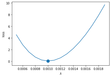
GIRL imitates the G-learner by minimizing a loss function over the state-action trajectories generated by the G-learner. The GIRL learned parameters in Table 1 are observed to be close to the G-learner parameters up to sampling error and numerical accuracy. GIRL is implemented using the ADAM method for stochastic gradient descent with a learning rate and a stopping tolerance on the parameter vector, . Consequently GIRL is observed to imitate the G-learner — the sample averaged portfolio returns closely track each other in Figure 2. The error in the learned G-learner parameters results in a marginal decrease in the Sharpe ratio, as reported in the parentheses of the legend in Figure 2. In Figure 3, we show the local behaviour of the loss surface for our problem, illustrating its convex shape and parameters found by GIRL. GIRL requires approximately 200 iterations to converge.
| Parameter | G-learner | GIRL |
|---|---|---|
| 0.4 | 0.406 | |
| 0.001 | 0.000987 | |
| 1.01 | 1.0912 | |
| 0.15 | 0.149 |

An illustration of an optimal solution trajectory obtained without enforcing any constraints is shown in Figure 4 which presents simulation results for the portfolio using the G-learner. The values of optimal cash installments are shown in Table 2.
 |
 |
| (a) | (b) |
 |
 |
| (c) | (d) |

| Period | Expected Cash Installments ($) |
|---|---|
| 1 | 0.0 |
| 2 | 73.384 |
| 3 | 85.7 |
| 4 | 97.36 |
| 5 | 113.083 |
| 6 | 129.889 |
| 7 | 153.362 |
| 8 | 181.832 |
| 9 | 207.472 |
| 10 | 237.292 |
| 11 | 275.926 |
| 12 | 318.154 |
| 13 | 360.212 |
| 14 | 420.546 |
| 15 | 495.813 |
| 16 | 563.691 |
| 17 | 638.042 |
| 18 | 716.391 |
| 19 | 787.57 |
| 20 | 861.794 |
| 21 | 954.392 |
| 22 | 1030.161 |
| 23 | 1106.024 |
| 24 | 1164.276 |
| 25 | 1190.959 |
| 26 | 1196.982 |
| 27 | 1173.541 |
| 28 | 1112.945 |
| 29 | 976.385 |
| 30 | 1416.265 |
7 Summary
To summarize, in this paper we presented a reinforcement learning (RL) based approach to problems of wealth management such as retirement plans. We used a generative framework for RL known as G-learning, and developed its practical implementation for both problems of optimization the policy given rewards (direct RL), and the inverse problem of finding the reward function of an agent from its observed behavior (inverse RL, or IRL). This resulted in two related practical algorithms that we called G-Learner and GIRL.
Our approach is applicable provided we use absolute (dollar-nominated) asset position changes as action variables, and choose a reward function which is quadratic in these actions. As shown in Sect. 4, G-learning with a quadratic reward and Gaussian reference policy gives rise to an entropy-regulated LQR as a novel tool for wealth management tasks. This approach results in a Gaussian optimal policy whose mean is a linear function of the state .
The method we presented enables extensions to other formulations including constrained versions or other specifications of the reward function. One possibility is to use the definition in Eq. (19) with the constraint in Eq. (20)), which provides an example of a non-quadratic concave reward. Such cases should be implemented using flexible function approximations for the action-value function such as neural networks.
By focusing on a semi-analytically tractable G-learning based approach to goal-based wealth management, we presented two practical algorithms that we called G-Learner and GIRL. As we showed using simulations where the “ground truth” is known, G-Learner is able to improve over the benchmark equally-weighted portfolio strategy, while GIRL is able to successfully recover parameters of an agent which is modeled as a G-Learner.
Given that behavioral data generated in our approach are very noisy (as it also happens in real financial markets), a success of such an endeavour could not be guaranteed beforehand, at neither stage. Indeed, the very ability of G-Learner to perform better than the benchmark equally-weighted portfolio is hinged, as could be expected, on the ability of the equity return model (the “alpha-model”) to exhibit some (rather weak) predictive power. Unlike a passive manager of the equally-weighted portfolio, the G-Learner is able to harvest the predictive power of the alpha model, providing a consistent boost in terms of resulting Sharpe ratio. Our numerical experiments demonstrate that the G-learner uses the alpha-model to consistently produce superior returns in a multi-period setting using a locally-quadratic reward function.
Furthermore, strong statistical noise in the data could also render the inverse problem of inference of the reward function of a G-Learner agent very difficult. As we demonstrated with experiments, however, GIRL manages to imitate the G-Learner, i.e. it infers the correct reward parameters, and thus imitates a G-Learner.
The two algorithms, G-Learner and GIRL, can be used either separately or in a combination. In particular, their combination could be used in robo-advising by modeling the actual human agents as G-learners, and then use GIRL to infer the latent objectives (rewards) of these G-learners. GIRL would then be able to imitate the best human investors, and thus could be offered as a robo-advising service to clients that would allow them to perform on par with best performers among all investors.
References
- Browne (1996) Browne, S. (1996). Reaching Goals by a Deadline: Digital Options and Continuous-Time Active Portfolio Management. https://www0.gsb.columbia.edu/mygsb/faculty/research/pubfiles/841/sidbrownedeadlines.pdf.
- Das et al. (2018) Das, S. R., D. Ostrov, A. Radhakrishnan, and D. Srivastav (2018). Dynamic Portfolio Allocation in Goals-Based Wealth Management. https://papers.ssrn.com/sol3/papers.cfm?abstractid=3211951.
- Dixon et al. (2020) Dixon, M. F., I. Halperin, and P. Bilokon (2020). Machine Learning in Finance: from Theory to Practice. Springer.
- Fox et al. (2015) Fox, R., A. Pakman, and N. Tishby (2015). Taming the Noise in Reinforcement Learning Via Soft Updates. 32nd Conference on Uncertainty in Artificial Intelligence (UAI), https://arxiv.org/pdf/1512.08562.pdf.
- Halperin and Feldshteyn (2018) Halperin, I. and I. Feldshteyn (2018). Market Self-Learning of Signals, Impact and Optimal Trading: Invisible Hand Inference with Free Energy, (or, How We Learned to Stop Worrying and Love Bounded Rationality). https://papers.ssrn.com/sol3/papers.cfm?abstract_id=3174498.
- Lagoudakis and Parr (2003) Lagoudakis, M. G. and R. Parr (2003). Least-Squares Policy Iteration. pp. 1107–1149. Journal of Machine Learning Research, 4.
- Lin et al. (2019) Lin, C., L. Zeng, and H. Wu (2019). Multi-period Portfolio Optimization in a Defined Contribution Pension Plan During the Decumulation Phase. pp. 401–427. Journal of Industrial and Management Optimization, 15(1)(doi:10.3934/jimo.2018059).
- Markowitz (1959) Markowitz, H. (1959). Portfolio Selection: Efficient Diversification of Investment. John Wiley.
- Merton (1971) Merton, R. C. (1971). Optimum Consumption and Portfolio Rules in a Continuous-Time Model. pp. 373–413. Journal of Economic Theory, 3(4).
- Sutton and Barto (2018) Sutton, R. S. and A. G. Barto (2018). Reinforcement Learning: An Introduction. Second edition, MIT.